Exploring Dependence Structures in the International Arms Trade Network

Abstract

In the paper we analyse dependence structures among international trade flows of major conventional weapons from 1952 to 2016. We employ a Network Disturbance Model commonly used in inferential network analysis and spatial econometrics. The dependence structure is represented by pre-defined weight matrices that allow for relating the arms trade flows from the network of international arms exchange. Several different weight matrices are compared by means of the AIC in order to select the best dependence structure. It turns out that the dependence structure among the arms trade flows is rather complex and can be represented by a specification that, simply speaking, relates each arms trade flow to all exports and imports of the sending and the receiving state. By controlling for explanatory variables we are able to show the influence of political and economic variables on the volume traded.

Keywords: Arms Trade; Dependence Structures; Model Selection; Network Disturbance Model; Network Analysis; Spatial Econometrics

1 Introduction

In this paper we investigate international trade flows of Major Conventional Weapons (MCW) using data provided by the Stockholm International Peace Research Institute (SIPRI). MCW include armoured vehicles, aircrafts, naval vessels etc. and SIPRI has collected all international arms transfers from 1950 to 2016 in a comprehensive database. The database includes information on the sending and the receiving country as well as the volume of the trades in a certain year. The volume is measured in so called TIV, shorthand for trend-indicator value(s), and represents the value of military resources that are exported. The data can be regarded as a year wise sequence of weighted networks where the countries are the nodes and the arms trade flows among them are the valued edges.

Several scholars have started to investigate arms trade using a network framework, but the available studies were restricted to binary relations, i.e. trade or no trade, see for example Willardson (2013), Akerman and Seim (2014), Kinne (2016) and Thurner et al. (2018). The central workhorse in inferential binary network analysis is thereby the Exponential Random Graph Model (ERGM), as introduced by Holland and Leinhardt (1981) (see also Frank and Strauss, 1986, Kolaczyk, 2009 and Lusher et al., 2012). Recent proposals for modelling valued networks within the ERGM class are provided by Krivitsky (2012) or the Generalized Exponential Random Graph Model (GERGM) by Desmarais and Cranmer (2012). The first model allows for discrete valued counts while in the GERGM the weights on the edges are transformed into interval data between zero and one. Both approaches are not suitable for modelling of arms trade data because the TIV is continuous and zero inflated (i.e. TIV$=0$ stands for no trade). Nonetheless, the binary analysis, i.e. trade or no trade, is central, since trading of arms implies governmental agreement and contracts and therefore represents direct and indirect trust relations, regardless of the amount of trading (see e.g. Jackson, 2010).

In this paper, however, we focus on the amount of trading (if there is trading). Of particular interest is thereby the dependence structure of trading amounts, that is how is the trading amount of a country (to a country) influenced by other trading amounts. In order to do so, we change the viewpoint of the network and go from a representation with the nodes as countries and the edges being arms trade flows to a network where the nodes are the trade flows between two countries and the edges represent the dependencies among them. This yields a model that at least conceptually resembles models from spatial econometrics (see e.g. LeSage and Pace, 2009 and Kauermann et al., 2012). This model class was developed for capturing spatial effects and spillovers from nearby sites and can be transformed to model the dependence of similar arms trade flows. Models from spatial econometrics even have their own name in the social network methodology and are commonly called Network Autocorrelation Models (see for example Leenders, 2002 and Hays et al., 2010).

The paper is organized as follows. In Section 2, we give a short description of the data, then in Section 3 we introduce our model and give different specifications and explanations for possible dependence structures. In Section 4 we present the results of our analysis. Section 5 concludes the paper.

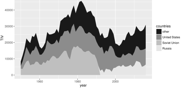
Figure 1: Development of exported TIV for 1950-2016 for the United States, Soviet Union, Russia and all other Countries.

2 Data description

The Stockholm International Peace Research Institute (SIPRI) is a unique data source on the international transfers of major conventional weapons. It covers more than 200 countries for the time period from 1950-2016 and includes information on the sending country, the receiving country as well as the type of MCW that is traded. Table 2 in Annex A.1 gives an overview of weapon systems included. SIPRI has developed a measure that represents arms trade flows as so called trend indicator values (TIV), based on production costs. The advantage of this measure is consistency over time and comparability of different arms systems. For detailed explanation of the data and methodology see SIPRI (2017b) or Holtom et al. (2012). The database can be accessed free of charge online at SIPRI (2017a).

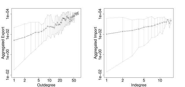
Figure 2: Log-Log Plot of TIV Export vs. Outdegree (left) and TIV Import vs. Indegree (right). Whiskers indicate minimum and maximum Values.

In Figure 1 the development of the aggregated TIV for the time period from 1950 to 2016 is shown for the two most important exporters United States and the Soviet Union (Russia since 1992). In Figure 2 a log-log plot of the outdegree and the aggregated export volume on the left and the indegree and the aggregated import volume on the right is given. The solid line in the middle gives the mean of exports or imports that is associated with the respective in- or outdegree, the whiskers indicate the maximum and the minimum value observed. In terms of the slope and range it can be seen that the connection between aggregated export volume and the outdegree is somewhat stronger than the connection between import volume and indegree. Nevertheless, both volumes increase on average in the degree.

3 Model

3.1 Definitions and Basic Formulation

In $T$ time periods, we observe $n_{t}$ flows $Y_{t}=\{Y_{t,ij}:Y_{t,ij}>0,i,j=1,....,N_{t}\}$ where $Y_{t,ij}$ is the valued arms trade flow from country $i$ to country $j$ among the $N_{t}$ countries that exist in $t=1,...,T$. In the following, we suppress the time index $t$ for ease of the notation. Let $V=\{(i,j):Y_{ij}>0\}$ be the (directed) index set for all country pairs $(i,j)$ where valued trade flows exists so that $Y=\{Y_{v}:v\in V\}$. Let $Y$ be of dimension $n=|V|$ and numerate the elements in $V$ so that $V=\{v_{1},...,v_{n}\}$.

As a tool to analyse the dependence structure amongst $Y$ we are using a graph $G$ consisting of nodes and edges, where we take $V$ as node set and define $E$ as symmetric edge set: $G=(V,E)$. We define the neighbourhood in the model through

$$\mathcal{N}(v_{a})\coloneqq\{v_{b}:\{v_{a},v_{b}\}\in E\}\text{, }a=1,...,n\text{.}$$

The information given in the neighbourhood can be summarized in a $(n\times n)$ matrix $\mathbf{W}$. Typically the rows of the matrix are normalized such that they sum up to one by defining $W_{ab}=|\mathcal{N}(v_{a})|^{-1}$ if $v_{b}\in\mathcal{N}(v_{a})$ and zero otherwise. This is also the definition we are using. As we are interested in the dependencies among arms trade flows we will henceforth attach the name tradecorrelation to the concept of related (neighbouring) flows. The intention of the subsequent analysis is to find a reasonable weight matrix $\mathbf{W}$, which defines an appropriate dependence structure.

3.2 Regression Model

Arms trade flows are non-negative, leading us to consider a multiplicative model of the form

$$\begin{split}\log(Y)&=\mathbf{x}^{\sf T}\boldsymbol{\beta}+u\\ (u_{1},...,u_{n})^{\sf T}=\mathbf{u}&\sim N_{n}(\mathbf{0},\mathbf{\Sigma}).\end{split}$$ (1)

Here $\mathbf{x}$ represents a vector of some covariates, $\boldsymbol{\beta}$ gives the parameter vector and $u$ is the error term. The residuals $\mathbf{u}$ are assumed to be correlated and $\mathbf{\Sigma}$ provides the variance-covariance matrix encoding the relation of different arms trade flows. Suitable candidates for estimation of (1) are models from spatial econometrics or spatial statistics, respectively. We will employ the former. Spatial econometric models are common in network analysis, see for instance Leenders (2002), Leifeld et al. (2016), Hays et al. (2010), Metz and Ingold (2017), Silk et al. (2017) and Ba (2017). We follow a Spatial Error Model (SEM, see LeSage and Pace, 2009) which is given by defining the error term $\mathbf{u}$ as

$$\begin{split}\mathbf{u}&=\rho\mathbf{W}\mathbf{u}+\boldsymbol{\epsilon},\\ \boldsymbol{\epsilon}&\sim N_{n}(\mathbf{0},\sigma^{2}\mathbf{I}_{n}),\end{split}$$ (2)

where $\mathbf{I}_{n}$ is the identity matrix of dimension $n$ and $\rho$ provides a measure for the dependency among the related error terms $\mathbf{u}$. The error terms $\boldsymbol{\epsilon}$ are assumed to be unstructured so that equation (2) can be reformulated to

$$\mathbf{u}=(\mathbf{I}_{n}-\rho\mathbf{W})^{-1}\boldsymbol{\epsilon}.$$ (3)

This implies the covariance matrix $\boldsymbol{\Sigma}=\sigma^{2}(\mathbf{I}_{n}-\rho\mathbf{W})^{-1}(\mathbf{I}_{n}-\rho\mathbf{W}^{\sf T})^{-1}$. Hence, matrix $\mathbf{W}$ expresses the dependence structure and the explicit choice of $\mathbf{W}$ is the central model selection task that will be discussed in Section 3.3. The modelling approach is also known as Network Disturbance Model (NDM) in the network literature, delegating the dependencies among trade flows into the error term. Hence, the approach does not aim to model a direct dependence between the trade flows but implies that the exogenous covariates determine the ”right” value for an arms trade flow, but one can find clusters of trade flows where the residuals are unusually high or low (see Leenders, 2002 and Freeman, 2017 for further discussion). We sketch some details on estimation and software in the Annex A.2.

3.3 Specifications of the Weight Matrix

We now focus on the central modelling task which is the appropriate specification of matrix $\mathbf{W}$ and hence the definition of the neighbourhood $\mathcal{N}$. We thereby focus on interpretable structures. Given that in the network context the weight matrices are rather abstract, we illustrate our approach with the arms trade network of the year 1952, being the simplest network under study. The network is shown in Figure 3. Note that all following illustrations of weight matrices $\mathbf{W}$ have their origin in the network shown in Figure 3 and are therefore not representative for other years. Still, they allow to visually understand the dependence structure.

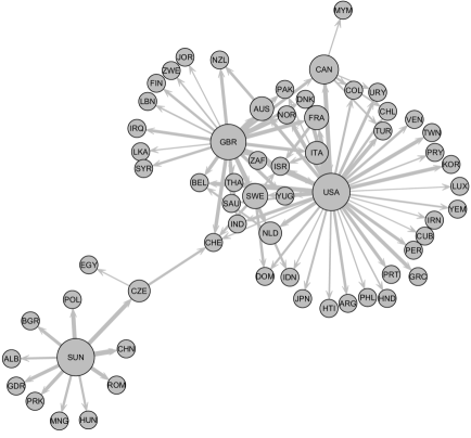
Figure 3: Directed valued Network of Arms Trade in 1952. Edges (Nodes) are scaled proportional to the logarithmic Exports (logarithmic aggregated Exports) measured in TIV.

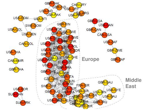
Figure 4: Tradecorrelation Structure 1. Colouring according to logarithmic TIV, ranging from Yellow (low) to Red (high).

Tradecorrelation 1 (attached to the Sending Country)

The first dependence structure relates an arms trade flow from country $i$ to country $j$ to all other exports going out of country $i$ and a possible reciprocal trade flow $(j,i)$. Notationally this means

$$\mathcal{N}_{1}((i,j))=\{(p,q):p=i\vee(p,q)=(j,i),(p,q)\in V\}.$$

The corresponding graph representation for the year 1952 is shown in Figure 4. The trade flows are grouped within clusters that are related to single exporting countries, most notably, the trade clusters of the big exporters: United States (USA), United Kingdom (GBR), Canada (CAN) and the Soviet Union (SUN). Via the dependence on reciprocal flows, the clusters are connected among each other if there is between-cluster trade. This explains the connection between the cluster of the United States (USA), Great Britain (GBR) and Canada (CAN). The trade activity of the Soviet Union (SUN), however, is disconnected.

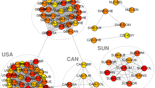
Figure 5: Tradecorrelation Structure 2. Colouring according to logarithmic TIV values, ranging from Yellow (low) to Red (high).

Tradecorrelation 2 (attached to the Receiving Country)

The concept from above can be amended such that the tradecorrelation of an arms trade is related to the trades of the importing country and not the exporting one. This means

$$\mathcal{N}_{2}((i,j))=\{(p,q):(p,q)=(j,i)\vee q=j,(p,q)\in V\}$$

and implies that the arms trade amount from $i$ to $j$ is correlated with other imports of $j$ as well as the potential reciprocal trade flow $(j,i)$. This is visualized in Figure 5. The resulting graph representation is very different from the previous one. There is no tendency of strong clustering as most importing countries do only have one or two suppliers and no exports at all which excludes connections via reciprocal flows. The greatest clusters consist of arms exports to Israel (ISR) and imports of Switzerland (CHE). Great Britain (GBR), United States (USA) and Canada (CAN) show their strong connections in arms trade by representing their own import-related cluster. Note that this structure disregards an important characteristic of the arms trade network: Receiving countries are often restricted to be dependent on one single exporter. Most important, trade flows of the Soviet Union (SUN) are missing.

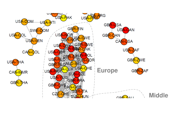
Figure 6: Tradecorrelation Structure 3. Colouring according to logarithmic TIV, ranging from Yellow (low) to Red (high).

Tradecorrelation 3 (attached to the Trade Activity of Sender and Receiver)

The structure of tradecorrelation 1 and 2 can be combined by the inclusion of the whole trade activity of $i$ and $j$, that is

$$\mathcal{N}_{3}((i,j))=\{(p,q):p\in\{i,j\}\vee q\in\{i,j\},(p,q)\in V\}.$$

In this case an arms trade from country $i$ to country $j$ is dependent on the whole trade activity of countries $i$ and $j$, regardless whether they are reciprocal or not. This results in a very dense graphical representation, as shown in Figure 6. Here, the clusters are again very clearly visible but the interconnection within and between clusters is much stronger. Central are the trade flows United States (USA) - Great Britain (GBR) and Great Britain (GBR) - United States (USA) as they link the two countries with the most trade activity. The flows related to Switzerland (CHE) serve as a bridge between the clusters around the western producers and the Soviet Union (SUN). With this specification the graph is connected and in principle each trade flow is allowed to be correlated with an arbitrary other arms trade flow.

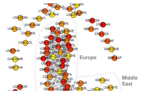
Figure 7: Tradecorrelation Structure 4. Colouring according to logarithmic TIV, ranging from Yellow (low) to Red (high).

Tradecorrelation 4 (related to Defence Agreements)

It can be discussed whether arms exchange is related to military alliances as they might agree to build up comparable military strength which potentially leads to correlated imports. The Correlates of War Project (2017a) provides data on formal alliances. We define a structure that relates the imports of country $j$ to imports of its allies. Let $da(j,i)=da(i,j)$ be an indicator that is one if countries $i$ and $j$ have a formal alliance. Then we define

$$\mathcal{N}_{4,import}((i,j))=\{(p,q):da(j,q)=1,(p,q)\in V\}.$$

This assumption imposes a structure where importers regard the arms imports of their allies when buying arms. In the corresponding plot in Figure 7 the trade clusters are not any longer attached to the sending countries but are rather clustered among countries that are connected in the alliances network. We see that the United States (USA), United Kingdom (GBR) and Canada (CAN) represent a (bipartite) cluster with their closest allies while the arms trade activity of the Soviet Union (SUN) forms a disconnected cluster. With this structure we additionally see a cluster containing the alliances of Canada (CAN), United Kingdom (GBR) and the United States (USA) together with countries from the Middle East. Naturally it is also possible to relate the exports of sending countries that have an alliance, resulting in

$$\mathcal{N}_{4,export}((i,j))=\{(p,q):da(i,p)=1,(p,q)\in V\}.$$

Figure 8: Tradecorrelation Structure 5. Colouring according to logarithmic TIV, ranging from Yellow (low) to Red (high).

Tradecorrelation 5 (related to Spatial Distance)

Using data provided by Gleditsch (2013a) we can incorporate spatial distances in the correlation structure. We assume that arms imports into spatially close areas are correlated and define $d(i,j)=d(j,i)$ as the distance between the two capital cities of $i$ and $j$. With $c$ representing a threshold we define

$$\mathcal{N}_{5,import}((i,j))=\{(p,q):j\neq q\wedge d(j,q)<c,(p,q)\in V\}.$$

Setting $c=1\,100$ km leads to spatially related trade activity clusters as shown in Figure 8, where in middle a cluster of tradeflows starts with countries from western Europe and relates them over eastern Europe to the Middle East. The choice of $c$ is discussed in the Annex A.3. Note that it is also possible to relate flows of spatially close exporters, that is

$$\mathcal{N}_{5,export}((i,j))=\{(p,q):i\neq p\wedge d(i,p)<c,(p,q)\in V\}.$$

3.4 Exogenous Covariates

We control for the influence from economics and politics by including additional covariates in model (1). Since there is an average time lag of roughly two years between ordering and delivering of weapons and some covariates are only available from 1950 on, the first network under study is the one of 1952 and covariates are lagged by two years.
Economic Quantities: The standard measure for economic size is the gross domestic product (GDP). We include this measure in logarithmic form for the sender as well as the receiver. The real GDP data is measured in thousands USD and are taken from Gleditsch (2013b). The data are merged from the year 2011 on with recent real GDP data from the World Bank real GDP dataset (see World Bank, 2017). It seems plausible that the military expenditures of the receiving countries are relevant. The data is available from Correlates of War Project (2017b) with Singer et al. (1972) as the basic reference for the data. As the time series for military expenditure ends in 2012 we have to assume that the values stay constant until 2014.
Political Quantities: We use a dummy variable being one if the countries $i$ and $j$ have a formal alliance and zero otherwise. Given the restriction that the data is available only until 2012 (Correlates of War Project (2017a) for the most recent version of the data and Gibler (2009) for the article of record for the data set) we assume that the alliances did not change between 2012 and 2015. In order to control for regime dissimilarity, we include the absolute difference of the so called polity score, ranging from the spectrum $-10$ (hereditary monarchy) to $+10$ (consolidated democracy). The data can be downloaded as annual time-series. See Marshall (2017) for the data and basic reference.

4 Results

4.1 Model Selection

Our ultimate goal is to select a suitable dependence model from above. As recommended by Leenders (2002) for this model class with several candidate weight matrices, we compare the proposed models using the Akaike Information Criteria (AIC) (see for example Claeskens and Hjort, 2008). For comparison we also include a simple linear model with unstructured error term (OLS, $\rho=0$). Estimation is done year wise and the AIC is calculated for all estimated models from 1952 to 2016, all in all covering $18\,964$ observations.

	$\mathcal{N}_{1}$	$\mathcal{N}_{2}$	$\mathcal{N}_{3}$	$\mathcal{N}_{4,import}$	$\mathcal{N}_{4,export}$	$\mathcal{N}_{5,import}$	$\mathcal{N}_{5,export}$	$\rho=0$
$\Delta_{i}$	$179.1$	$905.6$	$0.0$	$690.7$	$354.1$	$816.6$	$954.6$	$940.6$

•

Table 1: Difference between aggregated AIC Values and the minimum aggregated AIC Value for different Tradecorrelation Structures.

In Table 1 the results for the aggregated AIC, rescaled by the lowest one ($\Delta_{i}=$AIC${}_{i}-$AIC_min) are presented. AIC_min corresponds to tradecorrelation structure 3.

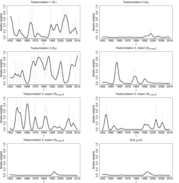
Figure 9: Year wise Akaike Weights for different Specifications (Raw Values in Gray, Smoothed in Black).

In order to investigate the different models more in detail, we also look at year wise AIC values. To do so, we compute Akaike weights, which can be interpreted as the probability of model $i$ being the best (i.e. minimizing the Kullback-Leibler Divergence given the data) among the proposed ones. The weights are given by $w_{i}=\exp(-\Delta_{i}/2)/(\sum_{r=1}^{R}\exp(-\Delta_{r}/2))$ (see Burnham and Anderson, 2004 for a further discussion). The weights are shown in Figure 9 for all eight specifications.

We see that the specification where $\rho$ is restricted to zero (OLS) is among those models that have a low probability of being the best one. Only in the years 1990-2000 the probability for this model rises slightly as a consequence of the collapse of the Eastern Bloc. Overall, this provides evidence for our initial hypothesis that the trade flows are indeed correlated.

Specification $\mathcal{N}_{5,export}$ (dependency of exports from spatially close countries), shows almost identical Akaike weights as the OLS specification. A plausible result, given that the capital cities of the big exporters United States and Soviet Union/Russia do not have nearby capital cities of other strong arms exporters and hence the greatest share of trade flows is restricted to be uncorrelated. This stands in contrast to $\mathcal{N}_{5,import}$ (dependency of imports of spatially close countries) that shows up to be among the better models in the beginning of the observational period and after 1989. Hence, this indicates that arms imports into spatially near countries are indeed related to some extent after 1989, which may be interpreted as a spatial clustering of arms imports.

While in tradecorrelation structure 5, the importer related assumption ($\mathcal{N}_{5,import}$) gives the higher probability to be the best one as compared to the exporter related assumption ($\mathcal{N}_{5,export}$), the opposite is the case for tradecorrelation structure 4, that is related to formal alliances. Here the model that assumes dependency of arms trade flows of allied exporting countries ($\mathcal{N}_{4,export}$) performs better than the one that relates those of allied importing countries ($\mathcal{N}_{4,import}$). This leads to the presumption that formal alliances mostly consist of partners with rather similar possibilities to export arms, i.e. either high ones, which leads to exports with high residuals or low ones, leading to exports with low residuals. The importers that are connected via formal alliances, seem to be more heterogeneous with respect to the height of their imports.

For the tradecorrelation structure 2 ($\mathcal{N}_{2}$, relating the imports and a potential reciprocal arms trade flow), we find a similar behaviour as for OLS and $\mathcal{N}_{5,export}$. Leading to the conclusion that there is no strong evidence that the importing arms flows are strongly correlated.

The two specifications that compete about being the best model are tradecorrelations $\mathcal{N}_{1}$ and $\mathcal{N}_{3}$. They alternate in being the best model in most time points. Mostly if the probability of the model with tradecorrelation $\mathcal{N}_{1}$ decreases, the one with tradecorrelation $\mathcal{N}_{3}$ increases and vice versa. But from a global perspective it is tradecorrelation $\mathcal{N}_{3}$ that provides the best model, which leads to the conclusion that a single arms trade flow is related to the whole trade activity of the sender as well as the receiver.

We infer that the exchange of international arms leads to a rather complex dependence structure. This shows that, similar to the binary analysis, the assumption of independent observations, given the covariates, is a strong simplification of the real process. Given this result we further analyse the model with tradecorrelation structure $\mathcal{N}_{3}$.

4.2 Coefficients

Tradecorrelation: The top left panel of Figure 10 shows the trade correlation coefficient using the structure $\mathcal{N}_{3}$. The coefficient is consistently positive but exhibits some variation. The strongest downward movement can be found in the years 1990 - 1996, showing how massively the end of the cold war altered the structure of the international trade of arms. From 1996 on, the coefficient increases again. In the most recent years the tradecorrelation fluctuates around $0.6$, close to the values before 1990.

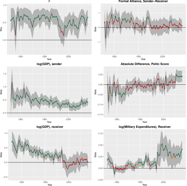
Figure 10: Time Series of Coefficients from the Model with Tradecorrelation Structure 3. $p$-values by colours (green $p<0.05$, orange $p<0.1$, red $p>0.1$). Shaded Regions give $\pm$ 2 standard deviations.

Economic Quantities: The coefficient on the logarithmic GDP of the sender is, with the exception of the year 1952, consistently positive and significant, showing a slight tendency to decrease with time. This can be seen from Figure 10, left panel, middle plot and reflects the fact that mostly wealthy countries have a highly developed arms industry which are able to produce and export expensive military equipment. The slight decrease of the coefficient is probably related to the increase of exporting countries that have smaller economic size. When it comes to the GDP of the receiver (left panel, bottom plot), we see a more pronounced downward trend of the coefficients. It is interesting to observe that from 1994 on, the coefficient becomes permanently insignificant. All in all there is no strong evidence that the TIV of arms imports is strongly influenced by the GDP of the receiving country since the 90s. It is, however influenced by the logarithm of military expenditure of the respective country as can be seen in the bottom plot of the right panel. There the coefficient on the logarithmic military expenditures is almost always positive since 1967 and mostly significant from 1990 on. This indicates a change in the arms trading mechanism. Before the end of the cold war, high arms trade flows went to countries with big economic size and after that, high flows are directed more strongly towards countries with high spending for military equipment.
Political Quantities: Before 1990, having an alliance (right panel, top plot) in tendency increased the amount of arms trading but at least since 1990 this effect is almost zero. The coefficient on the absolute differences of the polity score (right panel, middle plot) shows a time related trend. In the beginning (1953-1973) the coefficient is rather less than zero, giving the intuitive result that differences in political regimes reduce the amount of arms traded. From 1976 until 1991 the coefficient can be regarded as zero, which mirrors the fact that at the height of the cold war the belonging to a political bloc was more important then distances in the polity scores. After the end of the Soviet Union, the coefficient remained close to zero until 2011 where the coefficients becomes significantly positive for six consecutive years, providing the surprising result that differences in the polity score do not lead to a reduction of the traded amount of arms.

4.3 Residual Analysis

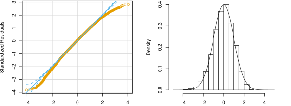
Figure 11: QQ-Plot (left) and Histogram (right) of standardized Residuals.

We give a graphical summary in Figure 11 for the pooled unstructured estimated residuals $\hat{\boldsymbol{\epsilon}}$. The plot on the left gives a QQ-plot with the quantiles of the standardized residuals on the vertical axes against the quantiles from a standard normal distribution on the horizontal axis. The right panel shows a histogram of the residuals together with a standard normal. Besides some irregularities in the tails, the results look quite acceptable.

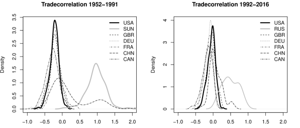
Figure 12: Kernel Density Estimates of the Tradecorrelation Residuals for selected Countries in the Time Periods 1952-1991 (left) and 1992-2016 (right).

As shown in the previous section, the coefficient on the tradecorrelation is always positive and it is therefore natural to ask whether it is possible to identify trade clusters with higher or lower than expected trade flows. In order to do so, we attribute to each country those elements of the vector of estimated ”tradecorrelation-residuals” ($\hat{\rho}\mathbf{W}\hat{\mathbf{u}}$) where the respective country is either the sender or the receiver. This is illustrated in Figure 12. For the periods 1952-1991 (left) and 1992-2016 (right) kernel density estimates of the the estimated ”tradecorrelation-residuals” for the most important countries are given. A strong difference in the distributions of the residuals can be found. Most notably the residuals are mostly negative for the United States (USA), Great Britain (GBR), Germany (DEU), France (FRA), and Canada (CAN) while the distribution for the Soviet Union (SUN) is shifted to the right and the one of China (CHN) is somewhat in-between In the period 1992-2016, the distributions are shifted closer together but the remarkable divide between the big western exporters and Russia (RUS) is still visible. This leads to the suggestion that the positive coefficient on tradecorrelation is partly driven by the differences of the tradeclusters of the western world and the one around the Soviet Union/Russia

5 Conclusion

In this paper we analysed the volume of international arms trade flows by employing a Network Disturbance Model. Seven different dependence structures are proposed and the best one is selected by the minimization of the AIC. Using this approach we find that a specification that relates the error term of an arms trade flow to the whole trade activity of the sending and receiving state works well in most years. This reveals that the network of international arms trade imposes a very complex dependence structure among the arms trade flows.

The analysis of the tradecorrelation coefficient shows that the correlation pattern among the flows rather stable and breaks only for the transition period after the end of the cold war. The development of the coefficients on the covariates shows how the influence of economic and political factors has changed with time.

Appendix A Annex

A.1 Descriptives

Table 2 gives the categories of arms that are included in the analysis. All types with explanations are taken from SIPRI (2017b). The 171 countries that are included in our analysis can be found in Table 3, together with the three-digit country codes that are used to abbreviate countries in the paper. In addition to that, the time periods, for which we coded the countries as existent are included. Note that the SIPRI data set contains more than 171 arms trading entities but we excluded non-states and countries with no (reliable) covariates available. In the covariates some missings are present in the data. No time series of covariates for the selected countries is completely missing (those countries are excluded from the analysis) and the major share of them is complete but there are series with some missing values. This is sometimes the case in the year $1990$ and/or $1991$ where the former socialist countries split up or had some transition time. In other cases values at the beginning or at the end of the series are missing. We have decided to impute the missing values via linear interpolation, using the R package imputeTS by Moritz (2016).

Type	Explanation
Aircraft	All fixed-wing aircraft and helicopters, including unmanned aircraft with a minimum loaded weight of 20 kg. Exceptions are microlight aircraft, powered and unpowered gliders and target drones.
Air-defence systems	(a) All land-based surface-to-air missile systems, and (b) all anti-aircraft guns with a calibre of more than 40 mm or with multiple barrels with a combined caliber of at least 70 mm. This includes self-propelled systems on armoured or unarmoured chassis.
Anti-submarine warfare weapons	Rocket launchers, multiple rocket launchers and mortars for use against submarines, with a calibre equal to or above 100 mm.
Armoured vehicles	All vehicles with integral armour protection, including all types of tank, tank destroyer, armoured car, armoured personnel carrier, armoured support vehicle and infantry fighting vehicle. Vehicles with very light armour protection (such as trucks with an integral but lightly armoured cabin) are excluded.
Artillery	Naval, fixed, self-propelled and towed guns, howitzers, multiple rocket launchers and mortars, with a calibre equal to or above 100 mm.
Engines	(a) Engines for military aircraft, for example, combat-capable aircraft, larger military transport and support aircraft, including large helicopters; (b) Engines for combat ships -,fast attack craft, corvettes, frigates, destroyers, cruisers, aircraft carriers and submarines; (c) Engines for most armoured vehicles - generally engines of more than 200 horsepower output.∗
Missiles	(a) All powered, guided missiles and torpedoes, and (b) all unpowered but guided bombs and shells. This includes man-portable air defence systems and portable guided anti-tank missiles. Unguided rockets, free-fall aerial munitions, anti-submarine rockets and target drones are excluded.
Sensors	(a) All land-, aircraft- and ship-based active (radar) and passive (e.g. electro-optical) surveillance systems with a range of at least 25 kilometres, with the exception of navigation and weather radars, (b) all fire-control radars, with the exception of range-only radars, and (c) anti-submarine warfare and anti-ship sonar systems for ships and helicopters.∗
Satellites	All reconnaissance and communications satellites.
Ships	(a) All ships with a standard tonnage of 100 tonnes or more, and (b) all ships armed with artillery of 100-mm calibre or more, torpedoes or guided missiles, and (c) all ships below 100 tonnes where the maximum speed (in kmh) multiplied with the full tonnage equals 3500 or more. Exceptions are most survey ships, tugs and some transport ships
Other	(a) All turrets for armoured vehicles fitted with a gun of at least 12.7 mm calibre or with guided anti-tank missiles, (b) all turrets for ships fitted with a gun of at least 57-mm calibre, and (c) all turrets for ships fitted with multiple guns with a combined calibre of at least 57 mm, and (d) air refueling systems as used on tanker aircraft.∗
∗In cases where the system is fitted on a platform (vehicle, aircraft or ship), the database only includes those systems that come from a different supplier from the supplier of the platform.
The Arms Transfers Database does not cover other military equipment such as small arms and light weapons (SALW) other than portable guided missiles such as man-portable air defence systems and guided anti-tank missiles. Trucks, artillery under 100-mm calibre, ammunition, support equipment and components (other than those mentioned above), repair and support services or technology transfers are also not included in the database.
Source: SIPRI (2017b)

Table 2: Types of Weapons included in the SIPRI Arms Trade Database

Country	Code	Included	Country	Code	Included	Country	Code	Included
Afghanistan	AFG	1950 - 2016	German Dem. Rep.	GDR	1950 - 1991	Pakistan	PAK	1950 - 2016
Albania	ALB	1950 - 2016	Germany	DEU	1950 - 2016	Panama	PAN	1950 - 2016
Algeria	DZA	1962 - 2016	Ghana	GHA	1957 - 2016	Papua New Guin.	PNG	1975 - 2016
Angola	AGO	1975 - 2016	Greece	GRC	1950 - 2016	Paraguay	PRY	1950 - 2016
Argentina	ARG	1950 - 2016	Guatemala	GTM	1950 - 2016	Peru	PER	1950 - 2016
Armenia	ARM	1991 - 2016	Guinea	GIN	1958 - 2016	Philippines	PHL	1950 - 2016
Australia	AUS	1950 - 2016	Guinea-Bissau	GNB	1973 - 2016	Poland	POL	1950 - 2016
Austria	AUT	1950 - 2016	Guyana	GUY	1966 - 2016	Portugal	PRT	1950 - 2016
Azerbaijan	AZE	1991 - 2016	Haiti	HTI	1950 - 2016	Qatar	QAT	1971 - 2016
Bahrain	BHR	1971 - 2016	Honduras	HND	1950 - 2016	Romania	ROM	1950 - 2016
Bangladesh	BGD	1971 - 2016	Hungary	HUN	1950 - 2016	Russia	RUS	1992 - 2016
Belarus	BLR	1991 - 2016	India	IND	1950 - 2016	Rwanda	RWA	1962 - 2016
Belgium	BEL	1950 - 2016	Indonesia	IDN	1950 - 2016	Saudi Arabia	SAU	1950 - 2016
Benin	BEN	1961 - 2016	Iran	IRN	1950 - 2016	Senegal	SEN	1960 - 2016
Bhutan	BTN	1950 - 2016	Iraq	IRQ	1950 - 2016	Serbia	SRB	1992 - 2016
Bolivia	BOL	1950 - 2016	Ireland	IRL	1950 - 2016	Sierra Leone	SLE	1961 - 2016
Bosnia Herzegov.	BIH	1992 - 2016	Israel	ISR	1950 - 2016	Singapore	SGP	1965 - 2016
Botswana	BWA	1966 - 2016	Italy	ITA	1950 - 2016	Slovakia	SVK	1993 - 2016
Brazil	BRA	1950 - 2016	Jamaica	JAM	1962 - 2016	Slovenia	SVN	1991 - 2016
Bulgaria	BGR	1950 - 2016	Japan	JPN	1950 - 2016	Solomon Islands	SLB	1978 - 2016
Burkina Faso	BFA	1960 - 2016	Jordan	JOR	1950 - 2016	Somalia	SOM	1960 - 2016
Burundi	BDI	1962 - 2016	Kazakhstan	KAZ	1991 - 2016	South Africa	ZAF	1950 - 2016
Cambodia	KHM	1953 - 2016	Kenya	KEN	1963 - 2016	Soviet Union	SUN	1950 - 1991
Cameroon	CMR	1960 - 2016	North Korea	PRK	1950 - 2016	Spain	ESP	1950 - 2016
Canada	CAN	1950 - 2016	South Korea	KOR	1950 - 2016	Sri Lanka	LKA	1950 - 2016
Cape Verde	CPV	1975 - 2016	Kuwait	KWT	1961 - 2016	Sudan	SDN	1956 - 2016
Central Afr. Rep.	CAF	1960 - 2016	Kyrgyzstan	KGZ	1991 - 2016	Suriname	SUR	1975 - 2016
Chad	TCD	1960 - 2016	Laos	LAO	1950 - 2016	Swaziland	SWZ	1968 - 2016
Chile	CHL	1950 - 2016	Latvia	LVA	1991 - 2016	Sweden	SWE	1950 - 2016
China	CHN	1950 - 2016	Lebanon	LBN	1950 - 2016	Switzerland	CHE	1950 - 2016
Colombia	COL	1950 - 2016	Lesotho	LSO	1966 - 2016	Syria	SYR	1950 - 2016
Comoros	COM	1975 - 2016	Liberia	LBR	1950 - 2016	Taiwan	TWN	1950 - 2016
DR Congo	ZAR	1960 - 2016	Libya	LBY	1951 - 2016	Tajikistan	TJK	1991 - 2016
Congo	COG	1960 - 2016	Lithuania	LTU	1990 - 2016	Tanzania	TZA	1961 - 2016
Costa Rica	CRI	1950 - 2016	Luxembourg	LUX	1950 - 2016	Thailand	THA	1950 - 2016
Cote dIvoire	CIV	1960 - 2016	Macedonia	MKD	1991 - 2016	Timor-Leste	TMP	2002 - 2016
Croatia	HRV	1991 - 2016	Madagascar	MDG	1960 - 2016	Togo	TGO	1960 - 2016
Cuba	CUB	1950 - 2016	Malawi	MWI	1964 - 2016	Trinidad Tobago	TTO	1962 - 2016
Cyprus	CYP	1960 - 2016	Malaysia	MYS	1957 - 2016	Tunisia	TUN	1956 - 2016
Czech Republic	CZR	1993 - 2016	Mali	MLI	1960 - 2016	Turkey	TUR	1950 - 2016
Czechoslovakia	CZE	1950 - 1991	Mauritania	MRT	1960 - 2016	Turkmenistan	TKM	1991 - 2016
Denmark	DNK	1950 - 2016	Mauritius	MUS	1968 - 2016	Uganda	UGA	1962 - 2016
Djibouti	DJI	1977 - 2016	Mexico	MEX	1950 - 2016	Ukraine	UKR	1991 - 2016
Dominican Rep.	DOM	1950 - 2016	Moldova	MDA	1991 - 2016	Un. Arab Emirates	ARE	1971 - 2016
Ecuador	ECU	1950 - 2016	Mongolia	MNG	1950 - 2016	United Kingdom	GBR	1950 - 2016
Egypt	EGY	1950 - 2016	Morocco	MAR	1956 - 2016	United States	USA	1950 - 2016
El Salvador	SLV	1950 - 2016	Mozambique	MOZ	1975 - 2016	Uruguay	URY	1950 - 2016
Equatorial Guin.	GNQ	1968 - 2016	Myanmar	MMR	1950 - 2016	Uzbekistan	UZB	1991 - 2016
Eritrea	ERI	1993 - 2016	Namibia	NAM	1990 - 2016	Venezuela	VEN	1950 - 2016
Estonia	EST	1991 - 2016	Nepal	NPL	1950 - 2016	Vietnam	VNM	1976 - 2016
Ethiopia	ETH	1950 - 2016	Netherlands	NLD	1950 - 2016	South Vietnam	SVM	1950 - 1975
Fiji	FJI	1970 - 2016	New Zealand	NZL	1950 - 2016	Yemen	YEM	1991 - 2016
Finland	FIN	1950 - 2016	Nicaragua	NIC	1950 - 2016	North Yemen	NYE	1950 - 1991
France	FRA	1950 - 2016	Niger	NER	1960 - 2016	South Yemen	SYE	1950 - 1991
Gabon	GAB	1960 - 2016	Nigeria	NGA	1960 - 2016	Yugoslavia	YUG	1950 - 1992
Gambia	GMB	1965 - 2016	Norway	NOR	1950 - 2016	Zambia	ZMB	1964 - 2016
Georgia	GEO	1991 - 2016	Oman	OMN	1950 - 2016	Zimbabwe	ZWE	1950 - 2016

Table 3: Countries included in the Analysis with three-digit Country Codes and Time-Period of Inclusion in the Model.

A.2 Technical Details on the Estimation

The estimation of the models is done in R (see R Development Core Team, 2014). For models with one weight matrix, there is an implementation by Bivand et al. (2013) (see also Bivand and Piras, 2015), based on a two-step method. First, the profiled likelihood is maximized with respect to $\rho$, by using the simplex method of Nelder and Mead (1965). In the second step the other parameters are found by weighted least squares. Given those estimates, the concentrated likelihood is updated for $\rho$. The major computational burden comes with the calculation of the log-determinant of $(\mathbf{I}_{n}-\rho\mathbf{W})$. The problem is solved by using the eigenvalues of $\mathbf{W}$, i.e. $\log(|\mathbf{I}_{n}-\rho\mathbf{W}|)=\sum_{i=1}^{n}\log(1-\rho\lambda_{i})$, with $\lambda_{i}$ being the eigenvalues of $\mathbf{W}$.

Further important packages used in this paper are the igraph package by Csardi and Nepusz (2006) as well as the statnet suite by Handcock et al. (2008) for the visualization of networks. For the Figures and Tables the packages ggplot2 by Wickham (2016) and stargazer by Hlavac (2013) are used.

A.3 Optimal Cutoff for the Spatial Distance

The optimal cutoff distances are found by maximization of Moran’s $I$ (see Moran, 1950) for the whole time period. In order to do so we construct a block-diagonal weight matrix for all observations and time periods and calculate Moran’s $I$ for varying threshold levels. The distance is discretized on a grid, ranging from $0$ km to $20\,000$ km, incrementing in steps of $100$ km. The highest value for Moran’s $I$ is found for $c=1\,100$ km for the weight matrix that relates the distances of the receiver ($\mathcal{N}_{5,import}$) and $c=300$ km for the weight matrix that relates the distances of the sender ($\mathcal{N}_{5,export}$). Note that we have chosen the maximum value in the sender-related model, although there is also a minimum value that is comparable in absolute numbers and could be interpreted as negative spatial correlation. This value is however realized for a cutoff value around $4\,600$ km which seems to be unrealistic (e.g. the distance between Moscow and London is roughly $2\,500$ km). The result is visualized in Figure 13.

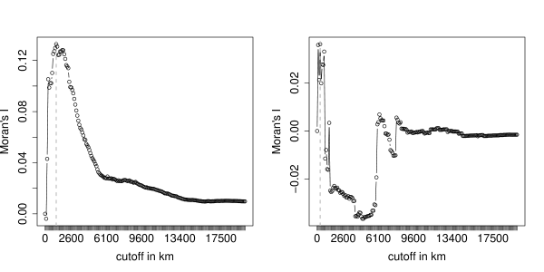
Figure 13: Moran’s $I$ for different Threshold Levels $c$ on a Grid. Receiver related Tradecorrelation on the left and Sender related Tradecorrelation on the right.

References

- Akerman and Seim (2014) Akerman, A. and A. L. Seim (2014). The global arms trade network 1950–2007. Journal of Comparative Economics 42(3), 535–551.
- Ba (2017) Ba, H.-L. K. (2017). Development, transition, and crisis in the international system, 1870-2009. Ph. D. thesis, The University of North Carolina at Chapel Hill.
- Bivand et al. (2013) Bivand, R., J. Hauke, and T. Kossowski (2013). Computing the jacobian in gaussian spatial autoregressive models: an illustrated comparison of available methods. Geographical Analysis 45(2), 150–179.
- Bivand and Piras (2015) Bivand, R. and G. Piras (2015). Comparing implementations of estimation methods for spatial econometrics. Journal of Statistical Software 63(18), 1–36.
- Burnham and Anderson (2004) Burnham, K. P. and D. R. Anderson (2004). Multimodel inference: understanding aic and bic in model selection. Sociological Methods & Research 33(2), 261–304.
- Claeskens and Hjort (2008) Claeskens, G. and N. L. Hjort (2008). Model selection and model averaging. Cambridge: Cambridge University Press.
- Correlates of War Project (2017a) Correlates of War Project (2017a). International military alliances, 1648-2012, version 4.1. http://www.correlatesofwar.org/data-sets/formal-alliances.
- Correlates of War Project (2017b) Correlates of War Project (2017b). National material capabilities, 1816-2012, version 5.0. http://www.correlatesofwar.org/data-sets/national-material-capabilities.
- Csardi and Nepusz (2006) Csardi, G. and T. Nepusz (2006). The igraph software package for complex network research. InterJournal, Complex Systems 1695(5), 1–9.
- Desmarais and Cranmer (2012) Desmarais, B. A. and S. J. Cranmer (2012). Statistical inference for valued-edge networks: The generalized exponential random graph model. PloS one 7(1), e30136.
- Frank and Strauss (1986) Frank, O. and D. Strauss (1986). Markov graphs. Journal of the American Statistical Association 81(395), 832–842.
- Freeman (2017) Freeman, L. C. (2017). Research methods in social network analysis. Routledge.
- Gibler (2009) Gibler, D. M. (2009). International military alliances, 1648-2008. Washington, DC: Congressional Quarterly Press.
- Gleditsch (2013a) Gleditsch, K. S. (2013a). Distance between capital cities. http://privatewww.essex.ac.uk/~ksg/data-5.html.
- Gleditsch (2013b) Gleditsch, K. S. (2013b). Expanded trade and gdp data. http://privatewww.essex.ac.uk/~ksg/exptradegdp.html.
- Handcock et al. (2008) Handcock, M. S., D. R. Hunter, C. T. Butts, S. M. Goodreau, and M. Morris (2008). statnet: Software tools for the representation, visualization, analysis and simulation of network data. Journal of Statistical Software 24(1), 1548–7660.
- Hays et al. (2010) Hays, J. C., A. Kachi, and R. J. Franzese (2010). A spatial model incorporating dynamic, endogenous network interdependence: A political science application. Statistical Methodology 7(3), 406–428.
- Hlavac (2013) Hlavac, M. (2013). stargazer: Latex code and ascii text for well-formatted regression and summary statistics tables. http://CRAN.R-project.org/package=stargazer.
- Holland and Leinhardt (1981) Holland, P. W. and S. Leinhardt (1981). An exponential family of probability distributions for directed graphs. Journal of the American Statistical Association 76(373), 33–50.
- Holtom et al. (2012) Holtom, P., M. Bromley, and V. Simmel (2012). Measuring international arms transfers. Stockholm International Peace Research Institute.
- Jackson (2010) Jackson, M. O. (2010). Social and economic networks. Princeton: Princeton University Press.
- Kauermann et al. (2012) Kauermann, G., H. Haupt, and N. Kaufmann (2012). A hitchhiker’s view on spatial statistics and spatial econometrics for lattice data. Statistical Modelling 12(5), 419–440.
- Kinne (2016) Kinne, B. J. (2016, may). Agreeing to arm. Journal of Peace Research 53(3), 359–377.
- Kolaczyk (2009) Kolaczyk, E. D. (2009). Statistical analysis of network data. Methods and Models. New York: Springer-Verlag.
- Krivitsky (2012) Krivitsky, P. N. (2012). Exponential-family random graph models for valued networks. Electronic Journal of Statistics 6, 1100–1128.
- Leenders (2002) Leenders, R. T. A. (2002). Modeling social influence through network autocorrelation: constructing the weight matrix. Social networks 24(1), 21–47.
- Leifeld et al. (2016) Leifeld, P., S. J. Cranmer, and B. A. Desmarais (2016). xergm: Extensions for Exponential Random Graph Models. R package version 1.6.2.
- LeSage and Pace (2009) LeSage, J. P. and R. K. Pace (2009). Introduction to spatial econometrics. London: Taylor and Francis.
- Lusher et al. (2012) Lusher, D., J. Koskinen, and G. Robins (2012). Exponential random graph models for social networks: Theory, methods, and applications. Cambridge: Cambridge University Press.
- Marshall (2017) Marshall, M. G. (2017). Polity iv project: Political regime characteristics and transitions, 1800-2016.
- Metz and Ingold (2017) Metz, F. and K. Ingold (2017). Politics of the precautionary principle: assessing actors’ preferences in water protection policy. Policy Sciences 50(4), 721–743.
- Moran (1950) Moran, P. A. (1950). Notes on continuous stochastic phenomena. Biometrika 37(1/2), 17–23.
- Moritz (2016) Moritz, S. (2016). imputeTS: Time Series Missing Value Imputation. R package version 1.6.
- Nelder and Mead (1965) Nelder, J. A. and R. Mead (1965). A simplex method for function minimization. The Computer Journal 7(4), 308–313.
- R Development Core Team (2014) R Development Core Team (2014). R: A Language and Environment for Statistical Computing. Vienna, Austria: R Foundation for Statistical Computing.
- Silk et al. (2017) Silk, M. J., D. P. Croft, R. J. Delahay, D. J. Hodgson, N. Weber, M. Boots, and R. A. McDonald (2017). The application of statistical network models in disease research. Methods in Ecology and Evolution 8(9), 1026–1041.
- Singer et al. (1972) Singer, J. D., S. Bremer, and J. Stuckey (1972). Capability distribution, uncertainty, and major power war, 1820-1965. Peace, War, and Numbers 19, 19–48.
- SIPRI (2017a) SIPRI (2017a). Arms transfers database. https://www.sipri.org/databases/armstransfers.
- SIPRI (2017b) SIPRI (2017b). Arms transfers database - methodology. https://www.sipri.org/databases/armstransfers/background.
- Thurner et al. (2018) Thurner, P. W., C. Skyler, G. Kauermann, and C. Schmid (2018). The network of major conventional weapons transfers 1950-2013. Ms. LMU Munich, submitted.
- Wickham (2016) Wickham, H. (2016). ggplot2: elegant graphics for data analysis. New York: Springer-Verlag.
- Willardson (2013) Willardson, S. L. (2013). Under the influence Of arms: the foreign policy causes and consequences of arms transfers. Ph. D. thesis, University of Iowa.
- World Bank (2017) World Bank (2017). World bank open data, real gdp. http://data.worldbank.org/.