Monte Carlo simulation for Ultra-cold neutron experiments searching for neutron - mirror neutron oscillation

Abstract

Neutron oscillation into mirror neutron, a sterile state exactly degenerate in mass with the neutron, could be a very rapid process, even faster than the neutron decay itself. It can be observed by comparing the neutron lose rates in an ultra-cold neutron trapping experiment for different experimental magnetic fields. We developed a Monte Carlo code that simulates many of the features of this kind of experiment with non-uniform magnetic fields. The aim of the simulation is to provide all necessary tools, needed for analyzing experimental results for neutron traps with different geometry and different configurations of magnetic field. This work contain technical details on the Monte Carlo simulation used for the analysis in Nostro not presented in it.

I Introduction

The concept of mirror world LY1 ; LY2 suggested long time ago for parity restoration attracted a considerable interest during last times (for reviews see refs. IJMPA1 ; IJMPA2 ; IJMPA3 ; IJMPA4 ). If mirror world exits, then all ordinary particles: the electron $e$, proton $p$, neutron $n$, photon $\gamma$, neutrinos $\nu$ etc. must have invisible twin degenerate in mass: $e^{\prime}$, $p^{\prime}$, $n^{\prime}$, $\gamma^{\prime}$, $\nu^{\prime}$ etc. which have no strong and electroweak interactions but, their own analogous interaction. It means that if ordinary particles are described by the Standard Model $G=SU(3)\times SU(2)\times U(1)$ or its extension, then mirror particle will be described by another copy of standard model $G^{\prime}=SU(3)^{\prime}\times SU(2)^{\prime}\times U(1)^{\prime}$ or its respective extension. Mirror matter interacting with ordinary matter via gravity provides an interesting and testable candidate for dark matter BDM1 ; BDM2 ; BCV1 ; BCV2 ; BCV3 ; BCV4 . However, particles of the two sectors can have some common interactions other then gravity PLB981 ; PLB982 ; PLB983 ; PLB984 ; PLB985 . Big Bang nucleosynthesis bounds and cosmological consistency on mirror dark matter require that these interactions should be rather feeble in order not to bring the two sector in thermal equilibrium in early universe BCV1 ; BCV2 ; BCV3 ; BCV4 . Nevertheless they can be important for dark matter direct detection DAMA1 ; DAMA2 ; DAMA3 ; DAMA4 . In addition, they can induce mixing phenomena between neutral ordinary and mirror particle, which could be testable.

For example, the three ordinary neutrinos $\nu_{e,\mu\,\tau}$ can oscillate into their mirror partners $\nu^{\prime}_{e,\mu\,\tau}$ which are in fact natural candidates for sterile neutrinos M-neutrinos1 ; M-neutrinos2 ; M-neutrinos3 ; M-neutrinos4 . This mixing can emerge via effective interactions which violate $B-L$ symmetries in both ordinary and mirror sectors. In the early Universe, these interactions would induce CP violating processes between ordinary and mirror particles which can co-generate baryon asymmetries in both sectors BB-PRL1 ; BB-PRL2 ; BB-PRL3 ; BB-PRL4 . In this way, one could naturally explain the relation $\Omega^{\prime}_{B}/\Omega_{B}\simeq 5$ between the baryon and dark matter fraction in the Universe BB-PRL1 ; BB-PRL2 ; BB-PRL3 ; BB-PRL4 ; IJMPA1 ; IJMPA2 ; IJMPA3 ; IJMPA4 .

As it was shown in refs. BB-nn' ; More , the oscillation between neutron $n$ and its mirror twin $n^{\prime}$, emerging due to the mass mixing term: $\epsilon(\bar{n}n^{\prime}+\bar{n}^{\prime}n)$, can be a fast process and it can be even faster than neutron decay. Energy conservation does not allow $n\to n^{\prime}$ transition in stable nuclei, and so, no limit emerges on the oscillation time from the nuclear stability BB-nn' . For free neutrons $n$–$n^{\prime}$ oscillation is influenced by matter and magnetic fields BB-nn' ; More . By that reason, existing experimental limits and astrophysical bounds still allow oscillation time $\tau=\epsilon^{-1}$ as small as few seconds BB-nn' , in drastic difference from the case of neutron-antineutron oscillation for which experimental lower bounds correspond to few years Phillips1 ; Phillips2 ; Phillips3 . It is interesting that $n\to n^{\prime}$ transitions faster than the neutron decay can have intriguing implications for the origin and propagation of ultra-high energy cosmic rays UHECR1 ; UHECR2 . In laboratory conditions, $n-n^{\prime}$ oscillations can be tested in experiments searching for neutron disappearance $n\to n^{\prime}$ and regeneration $n\to n^{\prime}\to n$ BB-nn' ; Pokot ; ORNL1 ; ORNL2 as well as via non-linear effects on the neutron spin precession More .

The ultra-cold neutron (UCN) storage experiments have good capabilities for testing the neutron disappearance phenomena. The status of presently existing UCN sources for fundamental physics measurements were recently reviewed in ref. Bison . In UCN traps the $n\to n^{\prime}$ oscillations can show up by measuring the magnetic field dependence of the UCN losses. In the last years, many UCN storage experiments were dedicated to search for $n-n^{\prime}$ oscillations Ban ; Serebrov ; Bodek ; Serebrov-New ; Altarev ; Nostro . The experiments Ban ; Serebrov ; Bodek ; Serebrov-New , compared the UCN loss rates in zero (i.e. small enough) and non-zero (large enough) experimental magnetic field assuming that the Earth has no mirror magnetic field BB-nn' . They obtained lower bounds on the oscillation time, with the strongest bound $\tau>414$ s at 90% CL of ref. Serebrov adopted by the Particle Data Group PDG .

These limits are not valid if there exists a non-vanishing mirror magnetic field $B^{\prime}$ at the Earth More . It would suppress $n-n^{\prime}$ oscillation even if the ordinary magnetic field is screened ($B=0$). On the other hand, if experimental magnetic field is tuned as $B\approx B^{\prime}$, then $n-n^{\prime}$ oscillation would be resonantly enhanced More . A detailed analysis of experimental data from Serebrov-New indicates towards more that $5\sigma$ deviation from the null hypothesis Berezhiani:2012rq which can be interpreted as a signal for $n-n^{\prime}$ oscillation with $\tau\sim 10$ s in the presence of mirror magnetic field $B^{\prime}\sim 0.1$ G. The mirror magnetic field at the Earth can emerge if the Earth captures some amount of mirror matter. Then, Earth rotation would drag mirror electrons inducing circular electric currents sourcing the mirror magnetic fields, which can be further amplified by dynamo mechanism More ; BDT . The experiment Altarev tested $n-n^{\prime}$ oscillation in the presence of mirror magnetic fields. Its results, gives the lower limit $\tau>12$ s for any $B^{\prime}$ less than 0.13 G. Somewhat stronger limits on $n-n^{\prime}$ oscillation parameters have been recently reported in Nostro . These limits Altarev ; Nostro restrict the parameter space which can be responsible for the above $5\sigma$ anomaly but do not cover it completely. Therefore new more precise experiment are needed to verify this anomaly.

To maximize the chances of finding a signal of $n-n^{\prime}$ oscillation in a UCN trap experiment, we have to apply the magnetic field as close as possible to the unknown mirror magnetic field. The most precise way would be to apply uniform magnetic field (as in the case of refs. Ban ; Serebrov ; Bodek ; Altarev and horizontal measurements of ref. Serebrov-New ) and to vary its value with very small steps for capturing the resonance. But such a procedure would require quite a long overall time of measurements. On the other hand, one could apply a non-uniform magnetic field (as in case of measurements with vertical magnetic field refs. Serebrov-New ; Nostro ). In this case, if the mirror field value falls within the spread of the applied magnetic field profile inside the trap, the neutrons moving in the trap with some probabilities cross this resonant areas where they oscillate very efficiently. This can give us some good possibility to catch the effect of the resonant amplification and give some gain in experimental time and statistics, since there will be no need to scan the magnetic field with very small steps.

This needs precise evaluation of oscillation probability for neutrons moving in non-uniform magnetic field. For this purpose we developed a Monte Carlo code and used it for the analysis of the results of the experiment Nostro . This tool was applied also to reinterpret the implications for parameter space from ref. Berezhiani:2012rq based on the analysis of the experiment Serebrov-New , since in Berezhiani:2012rq the non-uniformity of the magnetic field was not correctly taken into account and a specific empirical formula was used for averaging oscillation probability. As it was shown in Nostro , the non-homogeneity of the magnetic field substantially altered the relevant space for oscillation parameters.

In this paper we report the main features of the Monte Carlo code. It was written with the purpose of creating a tool that can be used in the analysis of any $n-n^{\prime}$ oscillation in a UCN trap experiment with non-uniform magnetic field and can be applied for material or magnetic UCN traps of different geometrical configurations. The paper is organized as follows: first we discuss $n-n^{\prime}$ oscillation in the presence of mirror magnetic field and the experimental setup. Then we describe key features of the simulation such as the UCN diffusion, wall scattering, loss probability and the behavior of $n-n^{\prime}$ oscillation probability. Finally we confront our results with the previous calculations and draw our conclusions.

II Neutron - Mirror Neutron Oscillations in Homogeneous Magnetic Field

Data form UCN experiment can be tested for magnetic field dependence of UCN losses, as a probe for $n-n^{\prime}$ oscillation. In fact, if free neutrons propagate through vacuum in a region where ordinary $\mathbf{B}$ and mirror $\mathbf{B}^{\prime}$ magnetic fields are both non-zero and have arbitrary orientation, the following Schrödinger equation with a $4\times 4$ Hamiltonian, describes $n-n^{\prime}$ oscillation phenomenology

$$\frac{d\Psi}{dt}=H_{nn^{\prime}}\Psi\;\;\;\;with\;\;\;\;H_{nn^{\prime}}=\left(\begin{array}[]{cc}\mu\mathbf{B}\cdot\mathbf{\sigma}&\epsilon\\ \epsilon&\mu\mathbf{B}^{\prime}\cdot\mathbf{\sigma}\end{array}\right)$$ (1)

where $\Psi=(\psi_{n}(t),\psi_{n^{\prime}}(t))$, is the wave function of $n$ and $n^{\prime}$ in two spin states, and $\mathbf{\sigma}=(\sigma_{x},\sigma_{y},\sigma_{z})$ are the Pauli matrices. Exact derivation of $n\to n^{\prime}$ transition probability is given in ref. More . Following Berezhiani:2012rq , in homogeneous fields $\mathbf{B}$ and $\mathbf{B}^{\prime}$, the probability of $n-n^{\prime}$ oscillation after neutron flight time $t$ can be reduced to:

$$P_{\mathbf{B}\mathbf{B}^{\prime}}(t)= \frac{\sin^{2}[(\omega-\omega^{\prime})t]}{2\tau^{2}(\omega-\omega^{\prime})^{2}}\left(1+\cos\beta\right)+$$

$$\frac{\sin^{2}[(\omega+\omega^{\prime})t]}{2\tau^{2}(\omega+\omega^{\prime})^{2}}\left(1-\cos\beta\right),$$ (2)

where $\beta$ is the angle between $\mathbf{B}$ and $\mathbf{B}^{\prime}$, and $\mu=-6\cdot 10^{-12}\,$eV/G being the neutron magnetic moment, and $\tau=\epsilon^{-1}$, $\omega=\frac{1}{2}|\mu B|$ and $\omega^{\prime}=\frac{1}{2}|\mu B^{\prime}|$. Given $B=|\mathbf{B}|$ and $B^{\prime}=|\mathbf{B}^{\prime}|$ the oscillation probability eq. (2) becomes maximal or minimal respectively when $\mathbf{B}$ and $\mathbf{B}^{\prime}$ are parallel or anti-parallel, $\cos\beta=\pm 1$:

$$P_{BB^{\prime}}^{(\pm)}(t)=\frac{\sin^{2}[(\omega\mp\omega^{\prime})t]}{\tau^{2}(\omega\mp\omega^{\prime})^{2}},$$ (3)

Experimental magnetic field can be controlled and thus the dependence of $n-n^{\prime}$ conversion probability on $\mathbf{B}$ can be tested. We can reverse magnetic field direction $\mathbf{B}\to-\mathbf{B}$ (i.e. $\beta\to\pi-\beta$) or measure counts with zero magnetic field. Therefore we can define:

$$D_{BB^{\prime}}\cos\beta \equiv\frac{P_{\mathbf{B}\mathbf{B}^{\prime}}-P_{-\mathbf{B}\mathbf{B}^{\prime}}}{2}$$

$$\mathcal{P}_{BB^{\prime}} \equiv P_{\mathbf{B}\mathbf{B}^{\prime}}+P_{-\mathbf{B}\mathbf{B}^{\prime}}$$

$$\mathcal{P}_{0B^{\prime}} \equiv P_{\mathbf{0}\mathbf{B}^{\prime}}.$$ (4)

$D_{BB^{\prime}}$ depend on $\beta$ and is non-zero only if $\cos\beta\neq 0$, while $\mathcal{P}_{BB^{\prime}}$ and $\mathcal{P}_{0B^{\prime}}$ are independent from the orientation of $\mathbf{B}$ and $\mathbf{B}^{\prime}$.

For trapped UCN, oscillation probability eq. (2) should be averaged over the distribution of neutron flight times $t$ between wall collisions. For averaging the sinusoidal factors in eq. (3) we can use the empirical formula from ref. Berezhiani:2012rq :

$$\langle\sin^{2}(\omega t)\rangle_{t}=S(\omega)=\frac{1}{2}\left[1-e^{-2\omega^{2}\sigma_{f}^{2}}\cos(2\omega t_{f})\right],$$ (5)

where $t_{f}=\langle t\rangle$ is the neutron mean free-flight time between wall collisions and $\sigma_{f}^{2}=\langle t^{2}\rangle-t_{f}^{2}$. is its variance. This parameters have to be computed via Monte Carlo simulation for each trap, depending on its geometry and size. Eq. (5) gives a correct asymptotic behavior for the average probabilities eq. (3):

$$\bar{P}_{BB^{\prime}}^{(\pm)}=\frac{S(\omega\mp\omega^{\prime})}{\tau^{2}(\omega\mp\omega^{\prime})^{2}}.$$ (6)

Calculation of $\bar{P}_{BB^{\prime}}$ with the analytic approximation eq. (5) agree at the level of percent to the one obtained via Monte-Carlo simulations if we consider a trap with homogeneous magnetic field.

As stated before, this oscillation phenomenon can be tested via magnetic field dependence of UCN losses. The regular UCN losses during the storage: $\beta$-decay, wall absorption or upscattering are magnetic field independent, so the number of neutrons $N(t_{\ast})$ survived after being stored in the trap for a certain time $t_{\ast}$ should not depend on $\mathbf{B}$, in the standard physics paradigm.

Nevertheless, if a neutron, between two consecutive wall collisions, oscillates into a mirror neutron state $n^{\prime}$, then per each collision it has some non-zero probability of escaping from the trap. Thus, the amount of survived neutrons in the UCN trap with applied magnetic field $\mathbf{B}$ after a time $t_{\ast}$ is given by $N_{\mathbf{B}}(t_{\ast})=N(t_{\ast})\exp(-n_{\ast}\bar{P}_{\mathbf{B}\mathbf{B}^{\prime}})$, where $\bar{P}_{\mathbf{B}\mathbf{B}^{\prime}}$ is the average probability of $n-n^{\prime}$ conversion between the wall scatterings and $n_{\ast}=n(t_{\ast})$ is the mean number of wall scatterings. If we reverse the magnetic field direction, $\mathbf{B}\to-\mathbf{B}$, then we have $N_{-\mathbf{B}}(t_{\ast})=N(t_{\ast})\exp(-n_{\ast}\bar{P}_{-\mathbf{B}\mathbf{B}^{\prime}})$. Since the common factor $N(t_{\ast})$ cancels in the neutron count ratios, asymmetry between $N_{\mathbf{B}}(t_{\ast})$ and $N_{-\mathbf{B}}(t_{\ast})$ is:

$$A_{\mathbf{B}}(t_{\ast})=\frac{N_{-\mathbf{B}}(t_{\ast})-N_{\mathbf{B}}(t_{\ast})}{N_{-\mathbf{B}}(t_{\ast})+N_{\mathbf{B}}(t_{\ast})}=n_{\ast}\bar{D}_{BB^{\prime}}\cos\!\beta\,,$$ (7)

assuming $n_{\ast}\bar{D}_{\mathbf{B}\mathbf{B}^{\prime}}\ll 1$. However, one can compare $N_{B}(t_{\ast})=\frac{1}{2}\big{[}N_{\mathbf{B}}(t_{\ast})+N_{-\mathbf{B}}(t_{\ast})\big{]}$ with the counts $N_{0}(t_{\ast})$ measured under zero experimental magnetic field:

$$E_{\mathbf{B}}(t_{\ast})=\frac{N_{0}(t_{\ast})-N_{\mathbf{B}}(t_{\ast})}{N_{0}(t_{\ast})+N_{\mathbf{B}}(t_{\ast})}=n_{\ast}(\bar{\mathcal{P}}_{BB^{\prime}}-\bar{\mathcal{P}}_{0B^{\prime}}),$$ (8)

$E_{\mathbf{B}}$ traces directly the difference between the probabilities in zero and non-zero magnetic fields. which depend only on its modulus $B=|\mathbf{B}|$, and it should be resonantly amplified if $B\approx B^{\prime}$. Since the parameter $n_{\ast}$ indicate the averaged number of wall collision for each UCN, its estimation it is very important for setting limits on the oscillation probability.

Measuring $E_{B}$ for many values of $B$, one can obtain limits on $n-n^{\prime}$ oscillation time $\tau$. On the other hand, from $A_{\mathbf{B}}$ one in fact measures the value $\tau_{\beta}=\tau/\sqrt{|\cos\beta|}$, i.e. oscillation time corrected by the unknown angle $\beta$ between ordinary and mirror magnetic fields $\mathbf{B}$ and $\mathbf{B}^{\prime}$. In ideal conditions, the effects of regular neutron loses cancel out from the ratios $A_{\mathbf{B}}$ and $E_{B}$, and measuring them for different values of $\mathbf{B}$, it is possible to obtain pretty robust limits on $\tau$ and $\tau_{\beta}$ as a function of mirror magnetic field $B^{\prime}$.

III Experimental Scheme

UCN experiment such as Serebrov ; Serebrov-New ; Nostro employed a trap of $190\,\ell$ volume capable of storing about half million neutrons, located inside a shield screening the Earth magnetic field. A controlled magnetic field is then induced by a system of solenoids. It can be oriented in both horizontal and vertical direction, but, in the vertical field setup it is not possible to have uniform magnetic field inside the trap. In this case, the induced magnetic field $\vec{B}$ has vertical direction practically everywhere inside the trap, but its magnitude $B=|\vec{B}|$ is in-homogeneously distributed, varying from the value $B_{c}$ in the geometrical center by about $\pm 0.5\,B_{c}$ at peripheral regions. The distribution of magnetic field inside the trap used in the experiment Nostro is shown in fig. 1.

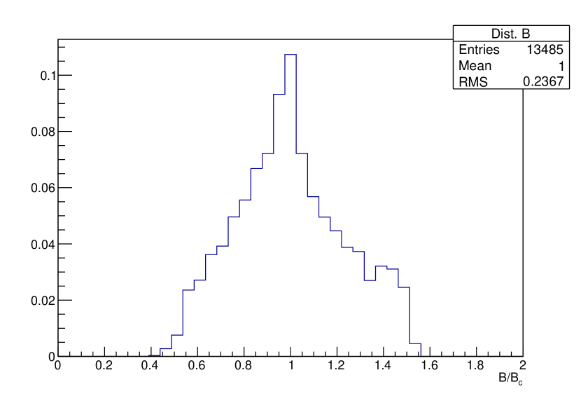
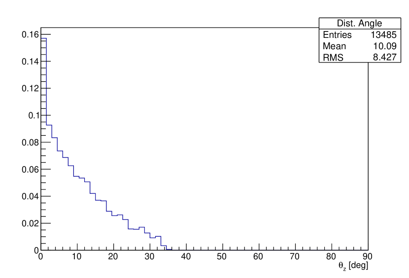
Figure 1: Magnetic field in the trap used in experiment Nostro . Upper panel: distribution of the absolute value of the magnetic field around the central value $B_{c}$. Lower panel: distribution of the deviation angles of vector $\vec{B}$ relative to $z$ axis.

The scheme of the installation used in the experiments Nostro is shown in Fig. 2.

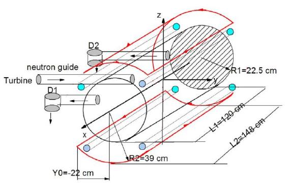
Figure 2: Scheme of the UCN trap used in Nostro ,the red lines, indicate the position of the electric circuits that generate vertical magnetic field inside the trap.

The trap used in Serebrov ; Serebrov-New ; Nostro is a horizontal cylinder with diameter 45 cm and length 120 cm. It was made of copper with the inner surface coated by beryllium. The critical velocity of this coating is 6.8 m/s which corresponds to the Beryllium optical potential: 2.7 $\times$ $10^{-7}$ eV. The magnetic shielding of the installation consists of four layers of permalloy, and the residual magnetic field inside the shielding is about 2 nT, which is low enough to carry out the search for $n-n^{\prime}$ transitions.

Every measurement, lasting about 10 minutes, consists of five phases: monitoring, filling, storage, emptying and background. In the monitor phase, the entrance valve is open and neutrons flow into the trap via the UCN guide while the exit valves that communicate with the two detectors $D_{1}$ and $D_{2}$ (fig. 2) remain open. Their counts during the monitor phase are used as estimators of the incident UCN flux and for checking its stability. Then the exit valves are closed for the filling phase, after which the entrance valve is closed and neutrons are kept in the trap for a storage time $t_{s}$. Then the exit valves are again opened and the survived UCN are counted by two detectors during the emptying phase. The final background phase checks that no excess of neutrons remains in the trap which could influence the following measurement.

IV UCN Motion

The program is written in C++ and implemented with ROOT, its core, consists in a simple numerical integration with the trapezoidal method of the motion of a single UCN that enters inside the trap from the UCN entrance (see fig. 2) with a randomly distributed velocity according to the UCN spectra from: UCN_spectra . Then it moves inside the trap under the effect of gravity acceleration for a certain storage time $t_{S}$. A key feature is the treatment of the collisions between UCN and the trap. The modification of the direction of motion induced by the elastic collision, combined with the discretization of time, induced an approximation error that grows with $t_{S}$ and manifest itself with a progressive loss of energy of the UCN. To avoid this, for each collision the squared module of the UCN neutron was computed imposing energy conservation:

$$v^{2}=2\left(E_{0}-gh\right)$$ (9)

where $E_{0}$ is the initial energy of the UCN normalized over the its mass, $v$ is its velocity, h is the height measured from the bottom of the trap and $g$ is gravity acceleration. With this trick we can have a good approximation even for $t_{S}>500$ s with an energy loss less then 1 %. Regarding UCN-trap scattering, half of them (randomly chosen) has been treated as specular scattering and the other half, as diffuse scattering UCN_reflection . In fig. 3 is shown a typical path of a simulated UCN.

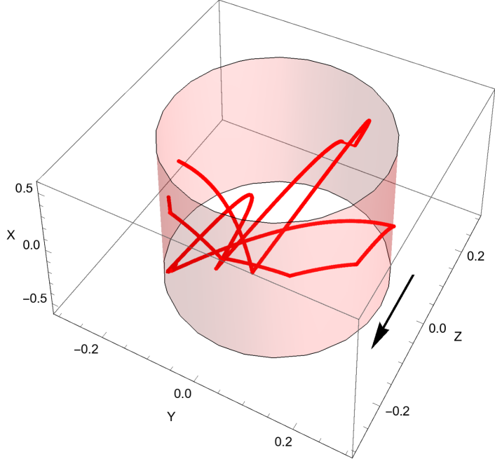
Figure 3: UCN path inside the trap. The black arrow indicates the orientation of gravity acceleration.

The escape probabilities $P_{esc}$ for each wall collision depends on the orthogonal component of the UCN velocity $v_{\bot}$ UCN_reflection ; Golub reads:

$$P_{esc}(v_{\bot})=2\,\eta\,\frac{|v_{\bot}|}{\sqrt{v_{max}^{2}-v_{\bot}^{2}}+2\eta\,|v_{\bot}|}$$ (10)

where $v_{max}=6.8$ m/s and $\eta$ are a parameters that depend on the material and the geometry of the trap, for the trap used in: Serebrov ; Serebrov-New ; Nostro we have $\eta\simeq 2.2\times 10^{-4}$. The $2\eta\,|v_{\bot}|$ term in the denominator has been added to avoid the probability to diverge when $v_{\bot}$ $\sim$ $v_{max}$. In the simulation we also take into account the $\beta$-decay, to this aim, in every numerical step each neutron has a decay probability given by $P_{\beta}$ = $dt/\tau_{n}$,where dt is the temporal step of the numerical integration and $\tau_{n}=(880.2\pm 1.0)$ s PDG is the free neutron mean lifetime. If a neutron decays or escapes during it’s motion inside the trap, it is discarded and not taken into account for the calculation of parameters of interest, because UCN lost for regular reasons are not relevant for the count asymmetry eq. (7) and (8). It is possible to study the coverage of the hits of UCN with the surface of the trap for different velocity classes. Results are shown in fig. 4, as it is easy to guess the coverage is not symmetric due to the effect of gravity, so especially for lower velocity class the coverage is higher in the bottom part of the trap. Coverage is important because, the value of magnetic field at the surface of the trap is the one the matter for $n\to n^{\prime}$ transition. With an in-homogeneous magnetic field, we have different values of $B$ for different regions, so, hitting the trap in the areas where the magnetic field have a value closer to the resonance will convert neutron more efficiently.

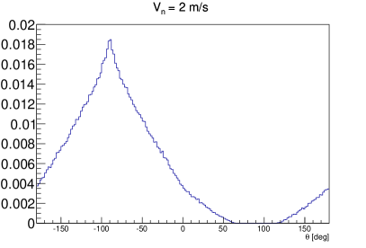
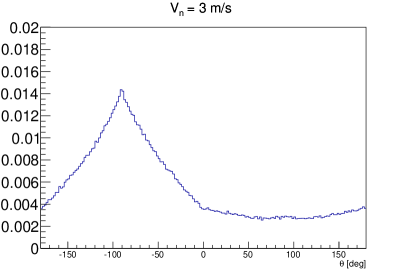
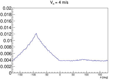
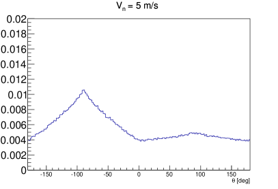
Figure 4: Coverage of UCN hits with the cylindric surface of the trap. Normalized distribution in terms of angles with the positive direction of the Y axis, for different velocity classes measured with $t_{S}$ = 100 s.

For the calculation of $n_{\ast}$, the code has been extended to simulate the three main phases of any measurements: filling, storage and emptying:

• Filling: In this phase, UCN are born at the entrance referring to fig. 2 and they move inside the trap for a randomly chosen time between 0 and $t_{F}$ with flat distribution, which is the experimental duration of the filling phase. If during this time interval the neutron decays, escapes or hit the entrance valve, it is considered as lost and not taken into account for the calculation of $n_{\ast}$. The entrance valve is a circular surface of 8 cm radius.

• Storage: UCN that survived the filling phase enter in the storage one. Here all entrance valves are closed, so they move inside the trap for a time $t_{S}$ and, as in the previous phase, if they decay or absorbed at the wall scattering, they are considered lost.

• Emptying: This is the counting phase, and it lasts for a certain time $t_{E}$. Only the UCN that in this phase hit the trap wall in correspondence of the two valves that are connected with the two detectors (see fig. 2), are considered counted and then taken into account for the calculation of $n_{\ast}$. The exit valves have the same shape and dimension of entrance valve. UCN that decay, escape or do not hit the exit valves during $t_{E}$ are again considered lost.

We first computed the mean value of free flight time $t_{\rm f}=\langle t\rangle$, its variance $\langle t^{2}\rangle$, etc. Their distribution were computed by averaging them over the individual UCN trajectories in the trap. The parameters $v_{max}$ and $\eta$ in eq. (10) were tuned to reproduce the experimental data such as the time constants for the neutron counts during the filling of the trap, UCN storage and the trap emptying. Our values are in good agreement with the parameters used in the previous experiments Serebrov ; Serebrov-New which used the same trap.

Now we have all the instruments to compute the averaged number of collision $n_{\ast}$ for each experimental configuration. We ran a thousand simulations per each experimental configuration, with $10^{5}$ neutron each, using the geometrical configuration of the trap of the experiments Serebrov ; Serebrov-New ; Nostro and computed the averaged number of wall collisions with the criteria stated above. Results are listed in table 1.

We estimated the uncertainties in the parameters $v_{max}$ and $\eta$ of eq. (10) to be 10% Ignatovich . Thus for each simulation we randomly generated their values from a Gaussian distribution which have the parameters used in Serebrov ; Serebrov-New , $\bar{v}_{max}=6.8m/s$ and $\bar{\eta}=2.2\times 10^{-4}$, as mean values and standard deviations given by: $\sigma_{v}=\bar{v}_{max}/10$ and $\sigma_{\eta}=\bar{\eta}/10$ respectively.

( Fill, Stor, Emt) [s]	$n_{*}$
( $100$, $250$, $150$)	2075 $\pm$ 86
( $130$, $300$, $130$)	2485 $\pm$ 103
( $100$, $150$, $240$)	1489 $\pm$ 58

Table 1: Results of Monte Carlo simulation in different time duration of the experimental phases: filling(Fill), storage(Stor) and emptying(Emt). The last line has been calculated using only one detector as in setup B4 of Nostro .

These numbers have been used to carry out the analysis in Nostro . The configuration of the second line in table 1 is the same as in the experiment described in Serebrov-New . In their simulation, reported also in Berezhiani:2012rq they found $n_{\ast}=4000$.

The discrepancy between our and their results can be explained by the fact that we directly computed the number of collisions per each neutron considering only neutrons that have actually been counted, while they calculated the UCN mean flight time $\langle t_{f}\rangle$ also including the not surviving neutrons and from that estimated $n_{\ast}$.

V Oscillation Probability

With an in-homogeneous experimental magnetic field, to set limits on the oscillation time, we cannot use the empirical formula used in Berezhiani:2012rq , that is valid only in case of a uniform magnetic field. We can use our simulation to estimate the dependence on the mirror magnetic field of the averaged value of the oscillation probability in the collision between UCN and the walls, in a specific experimental magnetic field configuration. For using this in the analysis of Nostro , we assumed that ordinary and mirror magnetic field are oriented in vertical direction. To this aim, during the motion of a UCN between two consecutive collisions, the Schroedinger equation eq. (1) has been numerically integrated.

The initial condition is set to have a neutron: $\Psi_{0}=(1,0)$, (pure neutron state), then, the wave function is computed in every temporal step using eq. (11). When the UCN hit the wall, the program computes and saves the current value of the oscillation probability $P=|\psi_{n^{\prime}}|^{2}$ and set $\Psi=\Psi_{0}$ back to the initial condition.

$$\psi_{n}(t_{i+1})= \cos\left(\delta\bar{\omega}_{i+1,i}\;dt\right)\psi_{n}(t_{i})$$

$$-i\sin\left(\delta\bar{\omega}_{i+1,i}\;dt\right)\cos 2\theta_{i+1,i}\;\psi_{n}(t_{i})$$

$$-i\sin\left(\delta\bar{\omega}_{i+1,i}\;dt\right)\sin 2\theta_{i+1,i}\;\psi_{n^{\prime}}(t_{i})$$

$$\psi_{n^{\prime}}(t_{i+1})= \cos\left(\delta\bar{\omega}_{i+1,i}\;dt\right)\psi_{n^{\prime}}(t_{i})$$

$$+i\sin\left(\delta\bar{\omega}_{i+1,i}\;dt\right)\cos 2\theta_{i+1,i}\;\psi_{n^{\prime}}(t_{i})$$

$$-i\sin\left(\delta\bar{\omega}_{i+1,i}\;dt\right)\sin 2\theta_{i+1,i}\;\psi_{n}(t_{i})$$ (11)

where

$$\delta\bar{\omega}_{i+1,i}= \;\sqrt{\delta\omega^{2}_{i+1,i}\,+\,\epsilon^{2}}$$

$$\delta\omega_{i+1,i}= \;(\omega_{i+1}+\omega_{i})/2-\omega^{\prime}$$

$$\sin 2\theta_{i+1,i}= \;\epsilon/\delta\bar{\omega}_{i+1,i}$$

$$\cos 2\theta_{i+1,i}= \;\delta\omega_{i+1,i}/\delta\bar{\omega}_{i+1,i}$$ (12)

and the mirror magnetic field $\omega^{\prime}$ (converted to the Larmor frequency) is assumed to be constant in the whole trap. On the other hand $\omega_{i}$ is the value of the ordinary magnetic field in the position of the UCN at time $t_{i}$. The magnetic field $\mathbf{B}$ was numerically calculated in every node of cubic lattice with 1 cm³ elementary volumes, and in this way the distributions shown in figs. 1 were obtained. In each elementary volume the magnetic field was taken as constant, with a value obtained by averaging between the values calculated at its vertices.

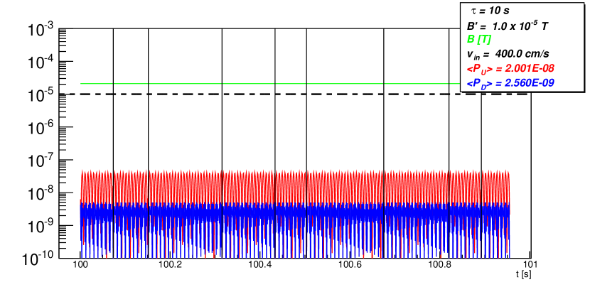
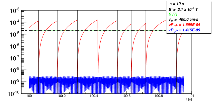
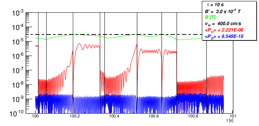
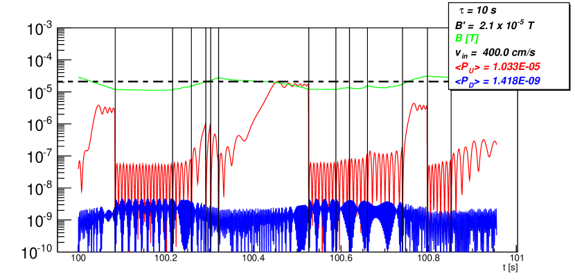
Figure 5: Examples of behavior of $P_{U}$ (red line) and $P_{D}$ (blue line) in four different ordinary and mirror magnetic field configurations for a UCN with 4 m/s velocity, assuming $\tau=10$ s. Black dashed line indicates $B^{\prime}$ while green line indicates B in the region in which UCN is moving. Each wall scattering is marked by a vertical black line. First panel: uniform ordinary magnetic field (B = 0.21 G) far from the resonance ($B^{\prime}$ = 0.1 G). Second panel: uniform ordinary magnetic at resonance ($B^{\prime}$ = B = 0.21 G) Third panel: not uniform ordinary magnetic field far from resonance ($B_{c}$ = 0.21 G and $B^{\prime}$ = 0.3 G). Fourth panel: not uniform ordinary magnetic field close to resonance ($B_{c}$ = 0.21 G and $B^{\prime}$ = 0.21 G).

Every UCN leaving an elementary cube with a given value of magnetic field with a wave vector $(\psi_{n},\psi_{n^{\prime}})$, while crossing the adjacent cube was evolving with the corresponding magnetic field. In fig. 5 we show some examples of the results of this calculation. We computed simultaneously, in every temporal step, the values of the probabilities $P_{U}$ and $P_{D}$ which represent respectively the cases where the ordinary and mirror magnetic field are parallel ($\beta=0$) or antiparallel ($\beta=\pi$). As it can be easily understood from fig. 5 as the UCN approaches to a region where the ordinary and mirror magnetic field are in resonance (same direction and magnitude) the probability grows up to $10^{-4}$ in the case of ideal resonance, with $\tau=10$ s.

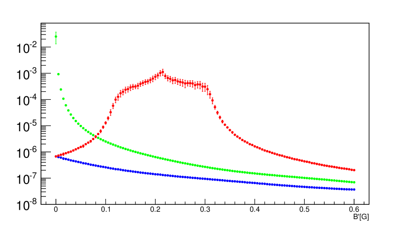
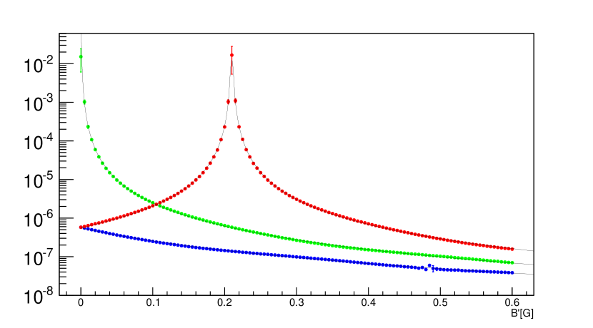
Figure 6: Results of the simulation with vertical not uniform magnetic field ($B_{c}$ = 0.21 G). Upper panel: in Red and blue we have, respectively, oscillation probability calculated in the case where B and $B^{\prime}$ are parallel ($\beta=0$) or antiparallel ($\beta=\pi$) i.e. $\mathcal{S}_{\pm}(B^{\prime})$. In green the case where B = 0 ($S_{0}(B^{\prime})$), error bars are given by the variance of the distributions (1 $\sigma$ ) for a given value of $B^{\prime}$. Lower panel:results of the simulation in the case of uniform experimental magnetic field (B = 0.21 G), compared with the e approximation used in Berezhiani:2012rq (Black lines).

Now we are able to study the dependence of the oscillation probabilities on the mirror magnetic field for a given profile of ordinary magnetic field. The UCN motion is integrated for 300 seconds in ideal conditions i. e. no $\beta$-decay and no trap losses to maximize hit statistics. Since we are interested in oscillation probabilities for only the UCN that are going to be detected, the UCN initial spectra in this simulation has been modified taking into account the fact that neutron with higher velocity escape from the trap after a small number of collisions due to eq. (10).

We computed mean values $P_{U}(B^{\prime})$ and $P_{D}(B^{\prime})$ of the oscillation probabilities eq. (3) between wall scatterings, averaged over distribution of the neutron flight time $t$ and distribution of the magnetic field $B$ in the trap for a given value of $B_{c}$, as functions of mirror magnetic field $B^{\prime}$. In addition, we computed also the mean oscillation probability $P_{0}(B^{\prime})$ for the case when no magnetic field was applied, $B=0$:

$$\bar{P}_{U/D}(B^{\prime}) =\left\langle\frac{\sin^{2}[(\omega\mp\omega^{\prime})t]}{\tau^{2}(\omega\mp\omega^{\prime})^{2}}\right\rangle_{t,B}=\left(\frac{1\,{\rm s}}{\tau}\right)^{2}\!\mathcal{S}_{\pm}(B^{\prime})\,,$$

$$\bar{P}_{0}(B^{\prime}) =\left\langle\frac{\sin^{2}(\omega^{\prime})t}{\tau^{2}\omega^{\prime 2}}\right\rangle_{t}=\left(\frac{1\,{\rm s}}{\tau}\right)^{2}\!\mathcal{S}_{0}(B^{\prime})\,.$$ (13)

In upper panel of fig. 6 we show simulation results for $\mathcal{S}_{\pm}(B^{\prime})$ and $\mathcal{S}_{0}(B^{\prime})$. These functions correspond to mean values of the respective probabilities in the case of $\tau=1$ s. For checking the consistency of our simulation, we also computed average oscillation probabilities in the case of homogeneous magnetic field in the same trap (lower panel of Fig. 6). As we see, the results of our simulation, coincide with the results obtained via the empirical formula eq. (5) for the corresponding values of the parameters $t_{\rm f}=\langle t\rangle$ and $\sigma^{2}_{\rm f}=\langle t^{2}\rangle-t_{\rm f}^{2}$, computed via our simulation.

From Fig. 6 we see that the in-homogeneous profile of the experimental magnetic fields has certain advantages: the function $\mathcal{S}_{+}(B^{\prime})$ in homogeneous magnetic field has maximal sensitivity at the resonance, $B\approx B^{\prime}$ as in the in-homogeneous case, but it is a very narrow resonance. So, if the variation of the field $B$ in search for the resonance is done with large steps, there is a chance to miss it. On the other hand, in the in-homogeneous field setup, the enhancement of the oscillation probability covers much wider range of values of $B^{\prime}$, and so, the search of the resonance can be done with larger steps, saving experimental time.

VI Conclusions

The aim of this work was to develop a tool that could be used in the analysis of any $n-n^{\prime}$ oscillation in a UCN trap experiment using a non-uniform magnetic field and for comparing results from different $n-n^{\prime}$ UCN oscillation experiments. The code has been used in the analysis presented in Nostro . The algorithm has been tested to maintain a good approximation up to 500 s UCN storage time with an energy loss less then 1 %. It has been developed for a cylindric trap, like the one used in Serebrov ; Serebrov-New ; Nostro , but it can be easily modified for a different geometrical configuration such us spheroidal traps and it can also simulate many different reflecting surfaces inside the trap. Unlike in the simulation used for Serebrov ; Serebrov-New , the calculation of the averaged number of collision $n_{\ast}$ have not taken into account all the UCN entering the trap, but only the ones that do not decay or escape until they have been counted by the detectors. We verified that the approximation for the calculation of oscillation probability used in Berezhiani:2012rq is well reproduced by our simulation assuming an uniform ordinary magnetic field inside the trap. The calculation of the $P_{U}$ and $P_{D}$ profiles show that experiments with not uniform magnetic field are sensitive to resonance in a larger set of $B^{\prime}$ values. So, this kind of configuration can be used in future experiments to scan a larger set of values for $B^{\prime}$ looking for resonance. Using this tools we could be able to compare UCN trapping experiment realized with different magnetic field, geometrical or technical setup. The code is available by contacting the author via email.

VII Acknowledgements

I want to thank Zurab Berezhiani and Nicola Rossi for useful discussions and technical support.

References

- (1) I. Y. Kobzarev, L. B. Okun and I. Y. Pomeranchuk, Sov. J. Nucl. Phys. 3, 837 (1966) [Yad. Fiz. 3, 1154 (1966)];
- (2) R. Foot, H. Lew and R. R. Volkas, Phys. Lett. B 272, 67 (1991).
- (3) Z. Berezhiani, Int. J. Mod. Phys. A 19, 3775 (2004) [hep-ph/0312335];
- (4) Z. Berezhiani, Eur. Phys. J. ST 163, 271 (2008);
- (5) Z. Berezhiani, In Shifman, M. et al. (eds.): From fields to strings, vol. 3, pp. 2147-2195, doi:10.1142/9789812775344-0055 [hep-ph/0508233];
- (6) R. Foot, Int. J. Mod. Phys. A 29, 1430013 (2014) [arXiv:1401.3965 [astro-ph.CO]].
- (7) Z. Berezhiani, A. D. Dolgov and R. N. Mohapatra, Phys. Lett. B 375, 26 (1996);
- (8) Z. G. Berezhiani, Acta Phys. Polon. B 27, 1503 (1996) [hep-ph/9602326].
- (9) Z. Berezhiani, D. Comelli and F. L. Villante, Phys. Lett. B 503, 362 (2001) [hep-ph/0008105];
- (10) A. Y. Ignatiev and R. R. Volkas, Phys. Rev. D 68, 023518 (2003) [hep-ph/0304260];
- (11) Z. Berezhiani, P. Ciarcelluti, D. Comelli and F. L. Villante, Int. J. Mod. Phys. D 14, 107 (2005) [astro-ph/0312605];
- (12) Z. Berezhiani, S. Cassisi, P. Ciarcelluti and A. Pietrinferni, Astropart. Phys. 24, 495 (2006) [astro-ph/0507153].
- (13) B. Holdom, Phys. Lett. 166B, 196 (1986);
- (14) Z. Berezhiani, Phys. Lett. B 417, 287 (1998);
- (15) Z. Berezhiani, L. Gianfagna and M. Giannotti, Phys. Lett. B 500, 286 (2001) [hep-ph/0009290].
- (16) A. Addazi, Z. Berezhiani and Y. Kamyshkov, Eur. Phys. J. C 77, no. 5, 301 (2017) [arXiv:1607.00348 [hep-ph]];
- (17) Z. Berezhiani, Eur. Phys. J. C 76, no. 12, 705 (2016) [arXiv:1507.05478 [hep-ph]].
- (18) R. Foot, Int. J. Mod. Phys. A 19, 3807 (2004) [astro-ph/0309330];
- (19) Phys. Rev. D 86, 023524 (2012) [arXiv:1203.2387 [hep-ph]];
- (20) R. Cerulli, et al., Eur. Phys. J. C 77, no. 2, 83 (2017) [arXiv:1701.08590 [hep-ex]];
- (21) A. Addazi, et al., Eur. Phys. J. C 75, no. 8, 400 (2015) [arXiv:1507.04317 [hep-ex]].
- (22) R. Foot, H. Lew and R. R. Volkas, Mod. Phys. Lett. A 7, 2567 (1992);
- (23) E. K. Akhmedov, Z. G. Berezhiani and G. Senjanovic, Phys. Rev. Lett. 69, 3013 (1992);
- (24) R. Foot and R. R. Volkas, Phys. Rev. D 52, 6595 (1995);
- (25) Z. Berezhiani and R. N. Mohapatra, Phys. Rev. D 52, 6607 (1995);
- (26) L. Bento and Z. Berezhiani, Phys. Rev. Lett. 87, 231304 (2001) [hep-ph/0107281];
- (27) L. Bento and Z. Berezhiani, Fortsch. Phys. 50, 489 (2002);
- (28) L. Bento and Z. Berezhiani, hep-ph/0111116;
- (29) Z. Berezhiani, arXiv:1602.08599 [astro-ph.CO].
- (30) Z. Berezhiani and L. Bento, Phys. Rev. Lett. 96, 081801 (2006) [hep-ph/0507031].
- (31) Z. Berezhiani, Eur. Phys. J. C 64, 421 (2009) [arXiv:0804.2088 [hep-ph]].
- (32) D. G. Phillips et al., Phys. Rept. 612, 1 (2016) [arXiv:1410.1100 [hep-ex]];
- (33) K. S. Babu et al., “Neutron-Antineutron Oscillations: A Snowmass 2013 White Paper,” arXiv:1310.8593 [hep-ex];
- (34) M. Baldo-Ceolin et al., Z. Phys. C 63, 409 (1994).
- (35) Z. Berezhiani and L. Bento, Phys. Lett. B 635, 253 (2006) [hep-ph/0602227];
- (36) Z. Berezhiani and A. Gazizov, Eur. Phys. J. C 72, 2111 (2012) [arXiv:1109.3725 [astro-ph.HE]];
- (37) Y. N. Pokotilovski, Phys. Lett. B 639, 214 (2006) [nucl-ex/0601017].
- (38) Z. Berezhiani et al.Phys. Rev. D 96, no. 3, 035039 (2017) [arXiv:1703.06735 [hep-ex]];
- (39) L. J. Broussard et al., arXiv:1710.00767 [hep-ex].
- (40) G. Bison et al., Phys. Rev. C 95, no. 4, 045503 (2017) [arXiv:1610.08399 [physics.ins-det]].
- (41) G. Ban et al., Phys. Rev. Lett. 99, 161603 (2007) [arXiv:0705.2336 [nucl-ex]].
- (42) A. P. Serebrov et al., Phys. Lett. B 663, 181 (2008) [arXiv:0706.3600 [nucl-ex]].
- (43) A. P. Serebrov et al., Nucl. Instrum. Meth. A 611, 137 (2009) [arXiv:0809.4902 [nucl-ex]].
- (44) K. Bodek et al., Nucl. Instrum. Meth. A 611, 141 (2009).
- (45) I. Altarev et al., Phys. Rev. D 80, 032003 (2009) [arXiv:0905.4208 [nucl-ex]].
- (46) Z. Berezhiani et al. arXiv:1712.05761 [hep-ex].
- (47) C. Patrignani et al. [Particle Data Group], Chin. Phys. C 40, no. 10, 100001 (2016).
- (48) Z. Berezhiani and F. Nesti, Eur. Phys. J. C 72, 1974 (2012) [arXiv:1203.1035 [hep-ph]].
- (49) Z. Berezhiani, A. D. Dolgov and I. I. Tkachev, Eur. Phys. J. C 73, 2620 (2013) [arXiv:1307.6953 [astro-ph.CO]].
- (50) A. Steyerl et al., Phys. Lett. A 116, 347 (1986).
- (51) F. Atchison et al., Nuclear Instruments and Methods in Physics Research A 552 (2005) 513–52
- (52) R. Golub and J. M. Pendlebury, Rept. Prog. Phys. 42, 439 (1979).
- (53) V.K. Ignatovich, The Physics of Ultracold Neutrons, Clarendon Press (1990), Oxford, UK