The nonparametric location–scale mixture cure model

Abstract.

We propose completely nonparametric methodology to investigate location–scale modelling of two–component mixture cure models, where the responses of interest are only indirectly observable due to the presence of censoring and the presence of so–called long–term survivors that are always censored. We use covariate-localized nonparametric estimators, which depend on a bandwidth sequence, to propose an estimator of the error distribution function that has not been considered before in the literature. When this bandwidth belongs to a certain range of undersmoothing bandwidths, the asymptotic distribution of the proposed estimator of the error distribution function does not depend on this bandwidth, and this estimator is shown to be root-$n$ consistent. This suggests that a computationally costly bandwidth selection procedure is unnecessary to obtain an effective estimator of the error distribution, and that a simpler rule-of-thumb approach can be used instead. A simulation study investigates the finite sample properties of our approach, and the methodology is illustrated using data obtained to study the behavior of distant metastasis in lymph-node-negative breast cancer patients.

Keywords: censored data, cure model, error distribution function, nonparametric regression

2010 AMS Subject Classifications: Primary: 62G08, 62N01; Secondary: 62G05, 62N02.

1. Introduction

A common problem faced in medical studies is for some subjects to never experience the event of interest during the study period. For example, consider a follow–up study examining the harmful side–effects of a pharmaceutical product. Since side–effects are commonly rare, it is expected that many subjects involved in the study will not experience the harmful effect of the treatment by the end of the study, and, therefore, these subjects will be censored at the conclusion of the study. Hence, these subjects are called long–term survivors. The first known study involving statistical analysis of data containing long–term survivors dates back to Boag (1949), and this author coined the term cure model to indicate the data contained a non–trivial proportion of long–term survivors. However, Farewell (1986) observes that cure models should not be used without clear empirical or biological need (see Section 2). Results on censored data models should be used in these cases, and studies involving subjects with censored responses are common. Well known methods can be employed to study these data (see, for example, Lawless, 1982; Aitkin et al.,1989; Harris and Albert, 1991; Collett, 1994).

We consider the case of observing responses $Y$ that are right censored by another random variable $C$, and, hence, observe only the minimum $Z=Y\wedge C$. Throughout this article, we will assume that $Y$ and $C$ are only conditionally independent given a covariate $X$, and, for simplicity, we will assume the censoring variable $C$ is a continuous random variable. For clarity, we will refer to responses corresponding to the subpopulation that has survival times that are finite as $Y_{u}$, which are only indirectly observed due to the presence of censored values. The purpose of this paper is to study the heteroskedastic nonparametric regression of $Y_{u}$ given the covariate $X$:

(1.1) $$Y_{u}=m(X)+s(X)\varepsilon.$$

Here $m$ is the regression function and $s$ is the scale function (bounded away from zero), which are both assumed to be smooth. We assume the error $\varepsilon$ is a continuous random variable that is independent of the covariate $X$ and has distribution function $F$. Identifiability of the components in the cure model also requires additional assumptions on the joint distribution of $(X,Z,\delta)$, where $\delta=\mathbf{1}[Y\leq C]$ is the right–censoring indicator. Finally, $m$ is assumed to be a location–type functional and $s$ is assumed to be a scale–type functional, which imposes additional requirements on the model error $\varepsilon$ that are analogous to the usual zero mean and unit variance assumptions so that we can identify both of $m$ and $s$ (see Section 2).

From the random sample of data $(X_{1},Z_{1},\delta_{1}),\ldots,(X_{n},Z_{n},\delta_{n})$ we will propose nonparametric function estimators of $m$, $s$ and $F$ in Section 2, and we study the large sample behavior of these estimators in Section 2.1. Note, these data also include the cured cases and, therefore, do not directly correspond with (1.1). Estimating the error distribution function $F$ is particularly important because many statistical inference procedures depend on functionals of $F$; for example, Kolmogorov–Smirnov–type and Cramér–von–Mises–type statistics. Van Keilegom and Akritas (1999) considered estimation of $F$, as well as the functions $m$ and $s$, from a model similar to (1.1) but without considering cured subjects, which presents a new and important challenge, and, hence, those results do not directly apply to the present situation.

We are interested in studying a completely nonparametric statistical methodology for examining location–scale modelling of data containing long–term survivors. Since the study of this type of data presented in Boag (1949), the literature on this subject has been divided into two distinct categories. The original cure model proposed by Boag (1949) is now known as the two–component mixture cure model (see, for example, Taylor, 1995). We will refer to the second category as simply the non–mixture cure model (see, for example, Haybittle, 1959, 1965). Several advancements have been made in the literature when these models are assumed to have a parametric or a semiparametric form. Kuk and Chen (1992) investigate combining logistic regression methods (used to estimate the unknown proportion of cured cases) with proportional hazards techniques to obtain estimators of their model parameters. Taylor (1995) works with a similar model as that of Kuk and Chen (1992) but proposes an Expectation-Maximization algorithm for simultaneously fitting the model parameters and estimating the baseline hazard function, and this author also uses simulations to conjecture that a crucial assumption is required for identifying components of these models (see Section 2). Sy and Taylor (2000) consider a similar model as that of Kuk and Chen (1992) but investigate an estimation technique based on the Expectation-Maximization algorithm. Lu (2008) considers the proportional hazards mixture cure model and proposes a semiparametric estimator of the unknown parameters of that model by maximizing a so-called nonparametric likelihood function. The estimator is shown to have minimum asymptotic variance. Lu (2010), the same author as before, investigates an accelerated failure time cure model (a special case of the two–component mixture cure model) and proposes an Expectation-Maximization algorithm for fitting the unknown parameters of that model as well as obtaining an estimator of the unknown error density function using a kernel-smoothed conditional profile likelihood technique. Xu and Peng (2014) and López-Cheda et al. (2017) consider estimating the unknown cure fraction in a completely nonparametric setting. Patilea and Van Keilegom (2017) consider a general approach to modelling the conditional survival function of a subject given that the subject is not cured by proposing so-called inversion formulae that allows one to express the conditional survival function of the uncured subjects in terms of the proportion of cured subjects and the subdistributions of the response and the censoring variable.

A particularly interesting model belonging to the non–mixture case is proposed by Yakovlev and Tsodikov (1996). Earlier, in a back-and-forth exchange over letters to the editors of Statistics in Medicine, Andrej Yakovlev very clearly details shortcomings of the two–component mixture cure model. Specifically, he argues that the two–component mixture cure model implicitly assumes that there is only a single risk operative in the population, i.e. a single latent variable that determines whether or not subjects are cured / uncured. Yakovlev argues that, in general, populations have multiple risk operatives and he proposes what we are referring to as the non–mixture cure model in his letter to the editors. The exchange between him and the authors Alan Cantor and Jonathan Shuster can be found in Yakovlev et al. (1994). Sometimes this model is called a promotion time cure model, and it has gained popularity due to motivations from Biology (in particular cancer research). Several results on parametric and semiparametric estimation of the unknown parameters in these models are available in the literature. However, this model is not in the scope of the current article, and we only mention a few of the notable works in this area. Tsodikov (1998) compares likelihood–based fitting techniques for the non–mixture cure model. Later, Tsodikov et al. (2003) survey the literature and report that, in less than a decade from its introduction, the non–mixture cure model is already in popular use, and these authors promote use of the non–mixture cure model in semiparametric and Bayesian settings. Zeng et al. (2006) propose a recursive algorithm for obtaining maximum likelihood estimates in the non–mixture cure model. Additionally, these authors show their regression parameter estimators have minimum asymptotic variance. Portier et al. (2017) consider an extension of the non–mixture cure model.

Recently, efforts have been made to unify the two seemingly distinct categories of cure models. Sinha et al. (2003) discuss the benefits and disadvantages of the mixture and non–mixture cure models. Yin and Ibrahim (2005) propose transforming the unknown population survival function in a manner that is analogous to the Box-Cox transformation for non-normally distributed random variables.

Our goal is to generally relax the model conditions and investigate an alternative estimation strategy for the two–component mixture cure model. A popular theme in both modelling categories is to use proportional hazards methods, where one estimates the baseline hazard function using a nonparametric estimator. In this case, the proportional hazards model is made additionally flexible through a nonparametric estimator of the baseline hazard function. The result is a semiparametric estimation technique (the remaining model parameters are finite dimensional and a likelihood function is usually required to obtain estimators).

The article is organized as follows. We further discuss model (1.1) and motivate our nonparametric function estimators in Section 2, and we give asymptotic results on these estimators in Section 2.1. In Section 3, we investigate the finite sample properties of our proposed estimator of $F$ and we illustrate the proposed techniques by characterizing a set of data collected to study distant metastasis in lymph-node-negative breast cancer patients. Our numerical study of the previous results in Section 3.1 shows the finite sample behavior of the estimators proposed in Section 2 is well–described by the asymptotic statements given in Section 2.1. The proofs of these results and further supporting technical results are given in Section 4.

2. Estimation of the model parameters

We begin this section with a discussion of the identifiability of the cure model parameters. In the following, write $G$ for the distribution function of the covariates $X$ and $g$ for the density function of $G$, where the support of $X$ is $[0,\,1]$. Let $Q$ be the conditional distribution function of the responses $Y$ given $X$ and $Q_{u}$ be the conditional distribution function of $Y_{u}$ given $X$. For both cure models and censored response models, it is important that we place conditions on the distribution function $Q$ (and therefore $Q_{u}$) so that we may identify and estimate the regression model components $m$ and $s$ and the error distribution function $F$. Empirical or biological need for using a cure model in the present situation means the support of the censoring variable $C$ is never contained in the support of the subpopulation $Y_{u}$, i.e. we require

(2.1) $$\tau_{0}=\sup_{x\in[0,\,1]}\tau_{u}(x)<\tau_{C}(x),\qquad x\in[0,\,1],$$

where $\tau_{u}(x)=\inf\{t\in\mathbb{R}\,:\,1-Q_{u}(t\,|\,x)=0\}$ and $\tau_{C}(x)=\inf\{t\in\mathbb{R}\,:\,P(C>t\,|\,X=x)=0\}$. Taylor (1995) uses simulation evidence to conjecture the necessity of (2.1). Xu and Peng (2014) and López-Cheda et al. (2017) observe that (2.1) leads to identifiability of the cure model components (see Lemma 1 of López-Cheda et al., 2017); specifically, it is required to identify the conditional proportion $\pi(X)$ of cured cases given $X$ as well as the conditional distribution function $Q_{u}$ of $Y_{u}$ given $X$. To ensure the distribution of the censoring variable $C$ is identifiable, we will further assume that the remaining mass of $Y$ beyond $\tau_{u}(X)$ occurs at $Y=\infty$, i.e. we assume the conditional equivalence of the events $\{Y>t\}=\{Y=\infty\}$, $t\geq\tau_{u}(X)$, given $X$. This justifies writing

$$P(Y>t\,|\,X)=\pi(X)+\{1-\pi(X)\}P(Y_{u}>t\,|\,X),\qquad t\in\mathbb{R},$$

where $\pi(X)=P(Y>\tau_{u}(X)\,|\,X)=P(Y=\infty\,|\,X)$ is assumed to be bounded away from zero and one, i.e. there are finite positive real numbers $0<\pi_{l}\leq\pi_{u}<1$ satisfying $\pi_{l}\leq\pi(X)\leq\pi_{u}$ for every $X$. Hence, $P(Y>\tau_{u}(X)\,|\,X)=\pi(X)=P(Y>\tau_{0}\,|\,X)$. This means that (2.1) implies that we only need an estimator of $\tau_{0}$, which does not depend on $X$, rather than $\tau_{u}(\cdot)$.

To conclude our discussion on identifiability, recall that the regression function $m$ is a location–type functional and the scale function $s$ is a scale–type functional. This means there are transformations $T$ and $V$ such that

$$m=T\big{(}Q_{u})=m+sT(F)\quad\text{and}\quad s=V(Q_{u})=sV(F).$$

Therefore, we can see that the regression model components $m$ and $s$ are identifiable when $T(F)=0$ and $V(F)=1$.

As noted on page 186 in Dabrowska (1987), responses arising from experiments with censored values are often skewed to the right and, therefore, estimators of the mean (and scale) will be affected. Beran (1981) proposes using $L$–type regression functionals, which are more robust to skewing in the data. To explain the idea, we introduce the score function $J$ and the quantiles $\xi_{u}(p\,|\,x)=Q_{u}^{-1}(p\,|\,x):=\inf\{y\in(-\infty,\,\tau_{0}]\,:\,Q_{u}(y\,|\,x)\geq p\}$ for $p\in[0,\,1]$. Here the score function $J$ must be nonnegative and satisfy $\int_{0}^{1}J(p)\,dp=1$. Throughout this article, we work with the following definitions of $m$ and $s$:

$$m(x)=\int_{0}^{1}\xi_{u}(p\,|\,x)J(p)\,dp\quad\text{and}\quad v(x)=\int_{0}^{1}\xi_{u}^{2}(p\,|\,x)J(p)\,dp-m^{2}(x),$$

where $s(x)=v^{1/2}(x)$ and $x\in[0,\,1]$. Hence, for $m$ and $s$ to be identifiable, we will require that $F$ satisfies

$$\int_{0}^{1}\xi_{F}(p)J(p)\,dp=0\quad\text{and}\quad\int_{0}^{1}\xi_{F}^{2}(p)J(p)\,dp=1,$$

where $\xi_{F}$ is the quantile function of $F$, i.e. $\xi_{F}(p)=\inf\{t\in\mathbb{R}\,:\,F(t)\geq p\}$ for $p\in[0,\,1]$.

With all of the components of the regression model (1.1) identified, we can define our estimators of the model parameters. To define the estimator of $Q$, we will introduce further notation. Write $M$ for the conditional distribution function of the minimum $Z$ given $X$ and $M^{1}$ for the conditional subdistribution function of both $Z$ and $\delta=1$ given $X$. From the discussion above, we can see that $\tau_{M}(x)=\inf\{t\in\mathbb{R}\,|\,P(Z>t\,|\,X=x)=0\}=\tau_{C}(x)>\tau_{0}$ for every $x$, which follows by (2.1), and, hence, we can consistently estimate $Q$ (and therefore $Q_{u}$) everywhere on the region $(-\infty,\,\tau_{0}]\times[0,\,1]$, cf. Van Keilegom and Akritas (1999).

Using $M$ and $M^{1}$, the conditional cumulative hazard function $\Lambda$ of $Y$ given $X$ may be written as

(2.2) $$\Lambda(t\,|\,X)=\int_{-\infty}^{t}\frac{Q(ds\,|\,X)}{1-Q(s-\,|\,X)}=\int_{-\infty}^{t}\frac{M^{1}(ds\,|\,X)}{1-M(s-\,|\,X)},\qquad t\in(-\infty,\tau_{0}].$$

To estimate $M$ and $M^{1}$, we introduce the Nadaraya–Watson weights

$$W_{j}(x)=K\bigg{(}\frac{x-X_{j}}{a_{n}}\bigg{)}\Bigg{/}\Bigg{\{}\sum_{k=1}^{n}K\bigg{(}\frac{x-X_{k}}{a_{n}}\bigg{)}\Bigg{\}},\qquad j=1,\ldots,n,$$

where $K$ is a given kernel function and $\{a_{n}\}_{n\geq 1}$ is a sequence of bandwidth parameters. Later, we will specify conditions on choosing $K$ and $\{a_{n}\}_{n\geq 1}$. Estimates of $M$ and $M^{1}$ then follow by the approach of Stone (1977): for $(t,\,x)\in(-\infty,\,\tau_{0}]\times[0,\,1]$,

(2.3) $$\hat{M}(t\,|\,x)=\sum_{j=1}^{n}\mathbf{1}(Z_{j}\leq t)W_{j}(x)\quad\text{and}\quad\hat{M}^{1}(t\,|\,x)=\sum_{j=1}^{n}\delta_{j}\mathbf{1}(Z_{j}\leq t)W_{j}(x).$$

Substituting (2.3) into (2.2) leads to an estimator of $Q$ in the approach of Beran (1981):

(2.4) $$\hat{Q}(t\,|\,x)=1-\prod_{Z_{(j)}<t}\bigg{\{}1-\frac{W_{(j)}(x)}{\sum_{k=j}^{n}W_{(k)}(x)}\bigg{\}}^{\delta_{(j)}},\qquad(t,\,x)\in(-\infty,\,\tau_{0}]\times[0,\,1].$$

Here $Z_{(1)}\leq\ldots\leq Z_{(n)}$ is the ascending ordering of $Z_{1},\ldots,Z_{n}$ and both of $\delta_{(1)},\ldots,\delta_{(n)}$ and $W_{(1)}(x),\ldots,W_{(n)}(x)$ are ordered according to $Z_{(1)},\ldots,Z_{(n)}$. For simplicity we will assume that the data contain no tied responses, which is reasonable because our assumptions imply the responses $Z_{j}$ are continuous random variables. Otherwise the ordering of the variables indicated above is not unique and the estimator $\hat{Q}$ is affected.

Xu and Peng (2014) propose estimating $\tau_{0}$ by the largest uncensored response $Z^{1}_{\text{max}}$ and then combining this estimator with (2.4) to form an estimator the unknown proportion $\pi$ of cured cases,

(2.5) $$\hat{\pi}(x)=1-\hat{Q}(Z^{1}_{\text{max}}\,|\,x),\qquad x\in[0,\,1].$$

The estimator $\hat{\pi}$ is shown to be consistent and asymptotically normally distributed. Later, López–Cheda et al. (2017) generalize this result in two steps. First, these authors show the estimator $Z^{1}_{\text{max}}$ is strongly consistent for $\tau_{0}$. Second, the estimator $\hat{\pi}$ is shown to be a uniformly, strongly consistent estimator of $\pi$.

Turning our attention now to $m$ and $s$, we can see that the unknown quantiles $\xi_{u}$ of the uncured population must be estimated. It is easy to show the equivalence $\xi_{u}(p\,|\,x)=\xi((1-\pi(x))p\,|\,x)$ from the equivalence $Q(\cdot\,|\,x)=\{1-\pi(x)\}Q_{u}(\cdot\,|\,x)$, with $p\in[0,\,1]$ and $x\in[0,\,1]$, where $\xi((1-\pi(x))p\,|\,x)=\inf\{y\in(-\infty,\,\tau_{0}]\,:\,Q(y\,|\,x)\geq\{1-\pi(x)\}p\}$. We can consistently estimate $\xi((1-\pi(x))p\,|\,x)$ by $\hat{\xi}((1-\hat{\pi}(x))p\,|\,x)$, where $\hat{\xi}((1-\hat{\pi}(x))p\,|\,x)=\inf\{y\in(-\infty,\,\tau_{0}]\,:\,\hat{Q}(y\,|\,x)\geq\{1-\hat{\pi}(x)\}p\}$. The resulting estimators of $m$ and $s$ are analogous to those of Van Keilegom and Akritas (1999):

$$\hat{m}(x)=\int_{0}^{1}\hat{\xi}\big{(}\big{(}1-\hat{\pi}(x)\big{)}p\,|\,x\big{)}J(p)\,dp\quad\text{and}\quad\hat{v}(x)=\int_{0}^{1}\hat{\xi}^{2}\big{(}\big{(}1-\hat{\pi}(x)\big{)}p\,|\,x\big{)}J(p)\,dp-\hat{m}^{2}(x),$$

with $\hat{s}(x)=\hat{v}^{1/2}(x)$, $x\in[0,\,1]$.

Write $\tau_{F}=\inf\{t\in\mathbb{R}:\,1-F(t)=0\}$ for the largest observable standardized error, which is finite by (2.1). It follows that $\{\tau_{u}(X)-m(X)\}/s(X)$ does not depend on $X$ and $\tau_{F}=\{\tau_{u}(X)-m(X)\}/s(X)$, for $G$–almost every $X$, from standardization. This means we can transfer the support of $F$, $(-\infty,\,\tau_{F}]$, into the support of $Q$, $(-\infty,\,\tau_{u}(x)]=(-\infty,\,\tau_{F}s(x)+m(x)]$, $x\in[0,\,1]$, where $Q$ can be estimated. Note, this is the same transfer of information from $F$ to $Q$ studied in Van Keilegom and Akritas (1999). However, this implies that we can form an estimator of $F$ using the estimators of $Q$, $\pi$, $m$ and $s$, which is new.

Observe the error distribution function $F$ can be written as the average

$$F(t)=E\bigg{[}\frac{Q(ts(X)+m(X)\,|\,X)}{1-\pi(X)}\bigg{]},\qquad-\infty<t\leq\tau_{F},$$

where we have used the transference mapping $t\mapsto ts(x)+m(x)$ for $-\infty<t\leq\tau_{F}$. We arrive at the proposed estimator of $F$:

(2.6) $$\hat{\mathbb{F}}(t)=\frac{1}{n}\sum_{j=1}^{n}\frac{\hat{Q}(t\hat{s}(X_{j})+\hat{m}(X_{j})\,|\,X_{j})}{1-\hat{\pi}(X_{j})},\qquad-\infty<t\leq\tau_{F}.$$

Note this estimator is averaging over the local model estimators at each covariate $X_{j}$ that are not consistent at the root-$n$ rate but are consistent at slower rates. Nevertheless, we show the estimator $\hat{\mathbb{F}}$ is root-$n$ consistent for $F$ and satisfies a functional central limit theorem (see Section 2.1).

2.1. Asymptotic results on the nonparametric function estimators

In order to state our asymptotic results for the estimators introduced in the previous section, we require the following assumptions:

1. The bandwidth $a_{n}$ satisfies $(na_{n}^{2})^{-1}\log\log(n)=O(1)$ and $na_{n}^{5}\log^{-1}(n)=O(1)$.

2. There are real numbers $0<\pi_{l}\leq\pi_{u}<1$ satisfying $\pi_{l}<\pi(X)<\pi_{u}$ for every $X$.

3. • The kernel function $K$ is a symmetric probability density function with support $[-1,\,1]$.

   • $K$ has bounded second derivative.

4. • The distribution function $G$ of the covariates $X$ has a density function $g$ that is bounded and bounded away from zero in $[0,\,1]$.

   • The density function $g$ has two bounded derivatives.

5. • There is a continuous nondecreasing function $L_{1}$ satisfying $L_{1}(-\infty)=0$ and $L_{1}(\tau_{0})<\infty$ such that

     $$M(t\,|\,x)-M(s\,|\,x)\leq L_{1}(t)-L_{1}(s),\qquad x\in[0,\,1],~{}-\infty<s<t\leq\tau_{0}.$$

   • The conditional (sub)distribution functions $M$ and $M^{1}$ have continuous partial derivatives, with respect to $x$, $\dot{M}$ and $\dot{M}^{1}$, respectively, that are bounded in $(-\infty,\,\tau_{c}]\times[0,\,1]$.

   • There are continuous nondecreasing functions $L_{2}$ and $L_{3}$ with $L_{2}(\tau_{0})<\infty$, $L_{3}(\tau_{0})<\infty$ and $L_{2}(-\infty)=L_{3}(-\infty)=0$ such that

     $$\dot{M}(t\,|\,x)-\dot{M}(s\,|\,x)\leq L_{2}(t)-L_{2}(s),\qquad x\in[0,\,1],~{}-\infty<s<t\leq\tau_{0},$$

     and

     $$\dot{M}^{1}(t\,|\,x)-\dot{M}^{1}(s\,|\,x)\leq L_{3}(t)-L_{3}(s),\qquad x\in[0,\,1],-\infty<s<t\leq\tau_{0}.$$

   • The second partial derivatives, with respect to $x$, of the conditional (sub)distribution functions $M$ and $M^{1}$ exist and are bounded in $(-\infty,\,\tau_{0}]\times[0,\,1]$.

6. The conditional distribution functions $M$ and $M^{1}$ admit bounded Lebesgue density functions.

7. The (conditional) distribution functions $P(Z\leq t)$ and $P(Z\leq t\,|\,\delta=1)$ are twice continuously differentiable and bounded away from zero in absolute value on any compact interval in the region $(-\infty,\,\tau_{0}]$, with the density function of $P(Z\leq t\,|\,\delta=1)$ bounded away from zero at $t=\tau_{0}$.

8. • The score function $J$ is bounded and nonnegative, and there are constants $0<p_{l}<p_{u}\leq 1$ such that $J$ is bounded away from zero on $(p_{l},\,p_{u})$ but equal to zero on $[0,\,p_{l}]\cup[p_{u},\,1]$ (when $p_{u}=1$ we only require that $J$ is equal to zero on $[0,\,p_{l}]$).

   • $J$ is continuously differentiable with bounded derivative $J^{\prime}$.

Assumptions (A3) and (A4) are common assumptions taken for nonparametric regression models, which guarantee good performance of nonparametric function estimators. Note that Assumptions (A5) (i) and (iii) are satisfied for many distributions. Suppose that $M$ is the logistic distribution function with a positive, bounded mean function $m(x)$ and scale function $s\equiv 1$. Write $l_{m}=\inf_{x}m(x)$ and $u_{m}=\sup_{x}m(x)$. Then Assumption (A5) (i) is satisfied by choosing $L_{1}(t)=\int_{-\infty}^{t}\,\exp(u_{m}-s)\{1+\exp(l_{m}-s)\}^{-2}\,ds$. When $m$ is also differentiable with a bounded derivative, then bounding functions $L_{2}$ and $L_{3}$ (that are similar to $L_{1}$) can be chosen to satisfy Assumption (A5) (iii) as well. Assumptions (A5) (ii) and (iv) and (A6) imply the conditional distribution functions $Q_{u}$ and $P(C\leq t\,|\,X)$ also meet these conditions and that $\pi$ must meet Assumptions (A5) (ii) and (iv), when these assumptions are required; e.g. due to the conditional independence of $Y$ and $C$ given $X$ we can write

$$1-M(t\,|\,X)=\big{[}\pi(X)+\{1-\pi(X)\}\{1-Q_{u}(t\,|\,X)\}\big{]}P(C>t\,|\,X).$$

In addition, $m$ and $s$ defined in Section 2 are functionals based on truncated means, which implies the integrals are restricted to compact subsets of $(-\infty,\,\tau_{0}]$. Therefore, combining the Leibniz integral rule for differentiation with Assumptions (A5) (ii) and (iv) yields that both $m$ and $s$ are twice differentiable with bounded derivatives. Assumption (A7) is a technical assumption required for the consistency of $Z^{1}_{\text{max}}$ for $\tau_{0}$, and many probability distributions satisfy this assumption as well. Finally, Assumption (A8) is a standard assumption that ensures $m$ and $s$ are well-defined $L$–type regression functionals (see page 186 of Dabrowska, 1987).

Define

$$\zeta\big{(}x,Z_{j},\delta_{j},t\big{)}=\frac{\delta_{j}\mathbf{1}[Z_{j}\leq t]}{1-M(Z_{j}-\,|\,x)}-\int_{-\infty}^{t}\frac{\mathbf{1}[Z_{j}>s]}{\{1-M(s-\,|\,x)\}^{2}}M^{1}(ds\,|\,x),\qquad j=1,\ldots,n.$$

Our first result specifies the asymptotic order and expansion of the estimator $\hat{\pi}$, which is given in Theorem 3 of López-Cheda et al. (2017). We offer an alternative proof of this result, which may be found in Section 4.

Proposition 1.

Let Assumptions (A1) – (A7) hold. Then

$$\sup_{x\in[0,\,1]}\big{|}\hat{\pi}(x)-\pi(x)\big{|}=O\big{(}(na_{n})^{-1/2}\log^{1/2}(n)\big{)},\qquad\text{a.s.}$$

Additionally,

$$\hat{\pi}(x)-\pi(x)=-\frac{\pi(x)}{g(x)}\frac{1}{na_{n}}\sum_{j=1}^{n}K\bigg{(}\frac{x-X_{j}}{a_{n}}\bigg{)}\zeta\big{(}x,Z_{j},\delta_{j},\tau_{0}\big{)}+R_{1,n}(x),$$

where $\sup_{x\in[0,\,1]}|R_{1,n}(x)|=O((na_{n})^{-3/4}\log^{3/4}(n))$, almost surely.

In the next two results, the asymptotic orders and expansions of the location estimator $\hat{m}$ and the scale estimator $\hat{s}$ are given.

Proposition 2.

Let Assumptions (A1) – (A7) and Assumption (A8) (i) hold. Then

$$\sup_{x\in[0,\,1]}\Big{|}\hat{m}(x)-m(x)\Big{|}=O\big{(}(na_{n})^{-1/2}\log^{1/2}(n)\big{)},\quad\text{a.s.}$$

Additionally, if Assumption (A8) (ii) holds,

$$\hat{m}(x)-m(x) =-\frac{1}{g(x)na_{n}}\sum_{j=1}^{n}K\bigg{(}\frac{x-X_{j}}{a_{n}}\bigg{)}\int_{-\infty}^{\tau_{0}}\,\zeta(x,Z_{j},\delta_{j},y)\frac{1-Q(y\,|\,x)}{1-\pi(x)}J\big{(}Q_{u}(y\,|\,x)\big{)}\,dy$$

$$\quad+\frac{\pi(x)}{1-\pi(x)}\frac{C_{m}(x)}{g(x)na_{n}}\sum_{j=1}^{n}K\bigg{(}\frac{x-X_{j}}{a_{n}}\bigg{)}\zeta(x,Z_{j},\delta_{j},\tau_{0})+R_{2,n}(x),$$

where $\sup_{x\in[0,\,1]}|R_{2,n}(x)|=O((na_{n})^{-3/4}\log^{3/4}(n))$, almost surely, and

$$C_{m}(x)=\int_{-\infty}^{\tau_{0}}\,Q_{u}(y\,|\,x)J\big{(}Q_{u}(y\,|\,x)\big{)}\,dy.$$

Proposition 3.

Let Assumptions (A1) – (A7) and Assumption (A8) (i) hold. Then

$$\sup_{x\in[0,\,1]}\Big{|}\hat{s}(x)-s(x)\Big{|}=O\big{(}(na_{n})^{-1/2}\log^{1/2}(n)\big{)},\quad\text{a.s.}$$

Additionally, if Assumption (A8) (ii) holds,

$$\hat{s}(x)-s(x) =-\frac{1}{g(x)na_{n}}\sum_{j=1}^{n}K\bigg{(}\frac{x-X_{j}}{a_{n}}\bigg{)}\int_{-\infty}^{\tau_{0}}\,\zeta(x,Z_{j},\delta_{j},y)\frac{1-Q(y\,|\,x)}{1-\pi(x)}\frac{y-m(x)}{s(x)}J\big{(}Q_{u}(y\,|\,x)\big{)}\,dy$$

$$\quad+\frac{\pi(x)}{1-\pi(x)}\frac{C_{s}(x)}{g(x)na_{n}}\sum_{j=1}^{n}K\bigg{(}\frac{x-X_{j}}{a_{n}}\bigg{)}\zeta(x,Z_{j},\delta_{j},\tau_{0})+R_{3,n}(x),$$

where $\sup_{x\in[0,\,1]}|R_{3,n}(x)|=O((na_{n})^{-3/4}\log^{3/4}(n))$, almost surely, and

$$C_{s}(x)=\int_{-\infty}^{\tau_{0}}\,Q_{u}(y\,|\,x)\frac{y-m(x)}{s(x)}J\big{(}Q_{u}(y\,|\,x)\big{)}\,dy.$$

To continue, it is common in heteroskedastic models to place a restriction on the curvature of the distribution function of either the responses or the errors (see, for example, Chown, 2016, who works with finite Fisher information for location and scale). Recall the functions $L_{1}$, $L_{2}$ and $L_{3}$ from Assumption (A5) (i) and (iii). We will require the function $L=L_{1}+L_{2}+L_{3}$ to satisfy the following curvature restriction that is analogous to assuming finite Fisher information for location and scale, i.e. we assume that $L$ has two derivatives such that

(2.7) $$\int_{-\infty}^{\tau_{0}}\big{(}1+v^{2}\big{)}\bigg{\{}\frac{L^{\prime\prime}(v)}{L^{\prime}(v)}\bigg{\}}^{2}\,L(dv)<\infty,\quad\int_{-\infty}^{\tau_{0}}\big{(}1+v^{2}\big{)}\,L(dv)<\infty\quad\text{and}\quad\sup_{-\infty<t\leq\tau_{0}}\big{|}tL^{\prime}(t)\big{|}<\infty.$$

Consequently, for sequences of real numbers $\{u_{n}\}_{n\geq 1}$ and $\{v_{n}\}_{n\geq 1}$ satisfying $u_{n}\to u$ and $v_{n}\to v$, as $n\to\infty$ and with $u,v\in\mathbb{R}$, (2.7) implies $|L(tv_{n}+u_{n})-L(tv+u)|=O(|u_{n}-u|+|v_{n}-v|)$, uniformly in $t$ (see the proof of Theorem 1 in Section 4). Note, (2.7) is also satisfied for many distributions, which includes the logistic distribution as in the example given above of a distribution satisfying Assumptions (A5) (i) and (iii). We are now prepared to state the two main results of this section: a strong uniform representation of the difference $\hat{\mathbb{F}}-F$ and the weak convergence of $n^{1/2}\{\hat{\mathbb{F}}-F\}$.

Theorem 1 (strong uniform representation of $\hat{\mathbb{F}}-F$).

Let Assumptions (A1) – (A8) hold. Assume the function $L=L_{1}+L_{2}+L_{3}$, where the functions $L_{1}$, $L_{2}$ and $L_{3}$ are given in Assumption (A5), is twice differentiable and satisfies (2.7). Finally, let $F$ satisfy (2.7), i.e. $F$ has finite Fisher information for both location and scale and the error density $f$ is bounded and satisfies $\sup_{-\infty<t\leq\tau_{F}}|tf(t)|<\infty$. Then

$$\hat{\mathbb{F}}(t)-F(t)=E_{n}(t)+R_{4,n}(t),$$

where $\sup_{-\infty<t\leq\tau_{F}}|R_{4,n}(t)|=O((na_{n})^{-3/4}\log^{3/4}(n))$, almost surely, and

$$E_{n}(t)=T_{n}(t)-f(t)\big{\{}U_{n}+tV_{n}\big{\}}-W_{n}(t)$$

with

$$T_{n}(t)=\frac{1}{n^{2}a_{n}}\sum_{1\leq j,k\leq n}K\bigg{(}\frac{X_{j}-X_{k}}{a_{n}}\bigg{)}\frac{1-Q(ts(X_{j})+m(X_{j})\,|\,X_{j})}{1-\pi(X_{j})}\frac{\zeta(X_{j},Z_{k},\delta_{k},ts(X_{j})+m(X_{j}))}{g(X_{j})},$$

$$U_{n}=\frac{1}{n^{2}a_{n}}\sum_{1\leq j,k\leq n}K\bigg{(}\frac{X_{j}-X_{k}}{a_{n}}\bigg{)}\frac{1}{g(X_{j})}\int_{-\infty}^{\tau_{0}}\,\zeta(X_{j},Z_{k},\delta_{k},y)\frac{1-Q(y\,|\,X_{j})}{1-\pi(X_{j})}J\big{(}Q_{u}(y\,|\,X_{j})\big{)}\,dy,$$

$$V_{n}=\frac{1}{n^{2}a_{n}}\sum_{1\leq j,k\leq n}K\bigg{(}\frac{X_{j}-X_{k}}{a_{n}}\bigg{)}\frac{1}{g(X_{j})}\int_{-\infty}^{\tau_{0}}\,\zeta(X_{j},Z_{k},\delta_{k},y)\frac{1-Q(y\,|\,X_{j})}{1-\pi(X_{j})}\frac{y-m(X_{j})}{s(X_{j})}J\big{(}Q_{u}(y\,|\,X_{j})\big{)}\,dy$$

and

$$W_{n}(t)=\frac{1}{n^{2}a_{n}}\sum_{1\leq j,k\leq n}K\bigg{(}\frac{X_{j}-X_{k}}{a_{n}}\bigg{)}\frac{\pi(X_{j})}{1-\pi(X_{j})}\frac{F(t)-f(t)\{C_{m}(X_{j})+tC_{s}(X_{j})\}}{g(X_{j})}\zeta(X_{j},Z_{k},\delta_{k},\tau_{0}).$$

Theorem 2 (weak convergence of $n^{1/2}\{\hat{\mathbb{F}}-F\}$).

Under the conditions of Theorem 1, if the bandwidth sequence $\{a_{n}\}_{n\geq 1}$ is chosen such that $a_{n}^{2}=o(n^{-1/2})$ and $(na_{n})^{-3/4}\log^{3/4}(n)=o(n^{-1/2})$ (e.g., $a_{n}=O(n^{-1/4-\gamma}\log^{1/4+\gamma}(n))$ for any $0<\gamma<1/12$) then $n^{1/2}\{\hat{\mathbb{F}}-F\}$ is asymptotically linear, i.e.

$$n^{1/2}\{\hat{\mathbb{F}}(t)-F(t)\}=n^{-1/2}\sum_{j=1}^{n}b_{t}(X_{j},Z_{j},\delta_{j})+R_{5,n}(t),$$

where $\sup_{-\infty<t\leq\tau_{F}}|R_{5,n}(t)|=o_{P}(1)$ and the influence function is

$$b_{t}(X_{j},Z_{j},\delta_{j}) =\frac{1-Q(ts(X_{j})+m(X_{j})\,|\,X_{j})}{1-\pi(X_{j})}\zeta\big{(}X_{j},Z_{j},\delta_{j},ts(X_{j})+m(X_{j})\big{)}$$

$$\quad-f(t)\int_{-\infty}^{\tau_{0}}\,\zeta\big{(}X_{j},Z_{j},\delta_{j},y\big{)}\frac{1-Q(y\,|\,X_{j})}{1-\pi(X_{j})}J\big{(}Q_{u}\big{(}y\,\big{|}\,X_{j}\big{)}\big{)}\,dy$$

$$\quad-tf(t)\int_{-\infty}^{\tau_{0}}\,\zeta\big{(}X_{j},Z_{j},\delta_{j},y\big{)}\frac{1-Q(y\,|\,X_{j})}{1-\pi(X_{j})}\frac{y-m(X_{j})}{s(X_{j})}J\big{(}Q_{u}\big{(}y\,\big{|}\,X_{j}\big{)}\big{)}\,dy$$

$$\quad-\frac{\pi(X_{j})}{1-\pi(X_{j})}\Big{[}F(t)-f(t)\big{\{}C_{m}(X_{j})+tC_{s}(X_{j})\big{\}}\Big{]}\zeta\big{(}X_{j},Z_{j},\delta_{j},\tau_{0}\big{)},$$

with $-\infty<t\leq\tau_{F}$. Consequently, the process $\{n^{1/2}\{\hat{\mathbb{F}}(t)-F(t)\}\,:\,-\infty<t\leq\tau_{F}\}$ weakly converges to a mean zero Gaussian process $\{Z(t)\,:\,-\infty<t\leq\tau_{F}\}$ with covariance function $\Sigma(t,v)=E[b_{t}(X,Z,\delta)b_{v}(X,Z,\delta)]$ for $-\infty<t,v\leq\tau_{F}$.

Remark 1 (consequences for the choice of bandwidth).

Theorem 2 implies that the estimator $\hat{\mathbb{F}}$ is a root-$n$ consistent estimator of $F$ only when the bandwidth sequence $\{a_{n}\}_{n\geq 1}$ satisfies $a_{n}^{2}=o(n^{-1/2})$ and $(na_{n})^{-3/4}\log^{3/4}(n)=o(n^{-1/2})$, which undersmoothes the estimators $\hat{Q}$, $\hat{m}$, $\hat{s}$ and $\hat{\pi}$. A bandwidth sequence given by $a_{n}=O(n^{-1/4-\gamma}\log^{1/4+\gamma}(n))$ satisfies $a_{n}^{2}=o(n^{-1/2})$ and $(na_{n})^{-3/4}\log^{3/4}(n)=o(n^{-1/2})$ for every $0<\gamma<1/12$. Note that when $\gamma=1/12$ we have $a_{n}=O(n^{-1/3}\log^{1/3}(n))$, and this choice does not lead to a root-$n$ consistent estimator because this bandwidth undersmoothes by too much. Alternatively, when $\gamma=0$ we have $a_{n}=O(n^{-1/4}\log^{1/4}(n))$, and this choice also does not lead to a root-$n$ consistent estimator because this bandwidth does not undersmooth by enough. Another interesting consequence highlighted by Theorem 2 is that the asymptotic behavior of $n^{1/2}\{\hat{\mathbb{F}}-F\}$ does not depend on the bandwidth sequence $\{a_{n}\}_{n\geq 1}$ used to construct the covariate-localized estimators when $a_{n}^{2}=o(n^{-1/2})$ and $(na_{n})^{-3/4}\log^{3/4}(n)=o(n^{-1/2})$.

3. Applications of the previous results

Here we investigate the finite sample properties of the proposed estimator $\hat{\mathbb{F}}$ using a simulation study. Our results indicate good finite sample behavior even at the smaller sample size of $100$ with multiple bandwidth configurations. This is particularly encouraging as we did not need to perform a computationally costly bandwidth selection procedure. Instead, we consider a variety of bandwidths of the form $C\hat{\sigma}_{X}n^{-1/4-\gamma}\log^{1/4+\gamma}(n)$, with parameters $C$ and $\gamma$ arbitrarily chosen and $\hat{\sigma}_{X}$ denoting the sample standard deviation of the covariates. The results given here reflect the conclusion in Remark 1: the estimator $\hat{\mathbb{F}}$ shows insensitivity to the choice of bandwidth parameters $\{a_{n}\}_{n\geq 1}$ used to construct the local model estimators when this sequence is chosen to appropriately undersmooth these estimators. This section is concluded with an illustration of the previous results using a dataset collected to study the behavior of distant metastasis in lymph-node-negative breast cancer sufferers.

3.1. Numerical study

To study the finite sample performance of the estimator $\hat{\mathbb{F}}$, we conducted simulations of $1000$ runs using sample sizes $100$, $200$, $500$ and $1000$ under the following data generation scheme. The covariates $X$ are uniformly distributed on the interval $[-1,\,1]$, and the location and scale functions are chosen as

(3.1) $$m(x)=1+2x+\frac{5}{4}\cos\big{(}\pi x^{2}\big{)}\quad\text{and}\quad s(x)=1+\frac{1}{2}\cos\big{(}\pi x\big{)},\qquad x\in[-1,\,1].$$

For the error distribution, we chose the standard normal distribution that has been truncated at 2, centered at zero and scaled to satisfy the cure model identifiability requirements (see Section 2). An initial set of responses $Y$ are then obtained using (1.1).

We work with a cure proportion function given by the logistic distribution function with standard scaling that has been centered at $7/4$, which gives about $16\%$ cured cases on average. Cure indicators are randomly generated based on this probability function, and whenever a cure indicator is equal to one we replace the corresponding value of $Y$ with $\infty$. Finally, the censoring variables $C$ are randomly generated from a mixture distribution of two components with equal mixing probabilities, where one component distribution is a normal distribution centered at $10$ with variation $1/2$ and the other component distribution is a shifted version of (1.1), with $m$ and $s$ as in (3.1) but now $m$ is shifted up by $1/2$ and the model errors are standard normally distributed (no truncation). These choices result in about $18\%$ censored values for the uncured cases. When we combine the censoring from both cases (cured and uncured) we expect a typical dataset generated in our simulations to present with about $31\%$ of censored response values.

The resulting response values $Z$ are taken as the minimum of each $Y$ and $C$ and a censoring indicator $\delta$ is set equal to one whenever $Y\leq C$ and zero otherwise. Finally, the score function $J$ is chosen by regions of $[0,\,1]$. In the region $(0.0001,\,1]$, $J$ is chosen as the logistic distribution function with scaling $0.0001$, and, in the region $[0,\,0.0001]$, $J$ is set equal to $0$. This is a smooth approximation of a step function that nearly integrates to $1$.

The bandwidth parameter sequence $\{a_{n}\}_{n\geq 1}$ used to construct the covariate-localized model estimators is of the form $a_{n}=C\hat{\sigma}_{X}n^{-1/4-\gamma}\log^{1/4+\gamma}(n)$, where $\hat{\sigma}_{X}$ denotes the sample standard deviation of the covariates $X$. We investigate four situations: the constant of proportionality $C$ is either $3/4$ or $9/8$ and the exponent parameter $\gamma$ is either $1/16$ or $1/28$. These choices are appropriate for Theorem 2, since $1/28<1/16<1/12$.

We numerically measure the performance of the estimator $\hat{\mathbb{F}}$ in two ways. First, the asymptotic mean squared errors at $t$-values $-2$, $-1$, $0$, $1$ and $2$ are simulated, where this performance metric is calculated by first obtaining the simulated mean squared errors and then multiplying these by the corresponding sample size. Second, the asymptotic integrated mean squared error is simulated, where this quantity is calculated similarly to the asymptotic mean squared errors but now we integrate over $t$. These performance metrics are predicted to be stable from Theorem 2.

$n$	$C,\,\gamma$	$-2$	$-1$	$0$	$1$	$2$
$100$	$3/4,\,1/16$	$0.014$	$0.046$	$0.078$	$0.054$	$0.003$
	$3/4,\,1/28$	$0.014$	$0.041$	$0.073$	$0.051$	$0.004$
	$9/8,\,1/16$	$0.015$	$0.030$	$0.082$	$0.038$	$0.006$
	$9/8,\,1/28$	$0.014$	$0.028$	$0.079$	$0.032$	$0.006$
$200$	$3/4,\,1/16$	$0.014$	$0.040$	$0.078$	$0.043$	$0.005$
	$3/4,\,1/28$	$0.014$	$0.036$	$0.070$	$0.037$	$0.006$
	$9/8,\,1/16$	$0.016$	$0.030$	$0.086$	$0.030$	$0.011$
	$9/8,\,1/28$	$0.017$	$0.026$	$0.095$	$0.032$	$0.009$
$500$	$3/4,\,1/16$	$0.015$	$0.035$	$0.088$	$0.040$	$0.009$
	$3/4,\,1/28$	$0.016$	$0.036$	$0.088$	$0.038$	$0.010$
	$9/8,\,1/16$	$0.019$	$0.032$	$0.099$	$0.031$	$0.018$
	$9/8,\,1/28$	$0.020$	$0.031$	$0.111$	$0.029$	$0.023$
$1000$	$3/4,\,1/16$	$0.017$	$0.043$	$0.093$	$0.047$	$0.012$
	$3/4,\,1/28$	$0.017$	$0.039$	$0.101$	$0.041$	$0.014$
	$9/8,\,1/16$	$0.019$	$0.034$	$0.109$	$0.032$	$0.026$
	$9/8,\,1/28$	$0.023$	$0.032$	$0.126$	$0.033$	$0.033$

Table 1. Simulated asymptotic mean squared error values of $\hat{\mathbb{F}}$ at the points $-2$, $-1$, $0$, $1$ and $2$.

	$100$	$200$	$500$	$1000$
$3/4,\,1/16$	$0.209$	$0.189$	$0.199$	$0.213$
$3/4,\,1/28$	$0.195$	$0.178$	$0.192$	$0.206$
$9/8,\,1/16$	$0.175$	$0.176$	$0.197$	$0.214$
$9/8,\,1/28$	$0.161$	$0.179$	$0.203$	$0.236$

Table 2. Simulated asymptotic integrated mean squared error values of $\hat{\mathbb{F}}$.

The results of the simulated asymptotic mean squared errors are displayed in Table 1, and the results of the simulated asymptotic mean integrated squared errors are given in Table 2. The values in Table 1 show the estimator $\hat{\mathbb{F}}$ has asymptotically stable pointwise mean squared errors (at the $t$-values $-2$, $-1$, $0$, $1$ and $2$), and this metric clearly shows the estimator $\hat{\mathbb{F}}$ to have good performance on samples as small as $100$. The values in Table 2 show a strong mirroring of the conclusions drawn from Table 1, which indicate that $\hat{\mathbb{F}}$ is a good estimator of $F$ even for samples as small as $100$.

We tried other bandwidth configurations and found similar results. However, in some cases, the performance metrics above were affected. Specifically, choosing the constant of proportionality $C$ either too large or too small showed the most significant effects while changing the exponent $\gamma$ showed no practical effect. We observed that choosing $C$ too large negatively impacted large sample behavior ($n=1000$) and choosing $C$ too small negatively impacted small sample behavior ($n=100$). This effect can be seen in Table 2 for the rows corresponding to $C=9/8$, but it is not very pronounced in this case. This indeed reflects the conclusions of Remark 1 that state the bandwidth should undersmooth but not undersmooth by too much. Nevertheless, the estimator $\hat{\mathbb{F}}$ does show insensitivity to the choice of bandwidth when this parameter is appropriately chosen. We therefore expect that a simple rule-of-thumb approach can be an effective strategy for choosing an appropriate bandwidth, where one (say) compares plots of several estimators of $F$ and chooses a bandwidth parameter among those that produced very similar estimators of $F$.

Summing up, we have numerically demonstrated that the estimator $\hat{\mathbb{F}}$ has good finite sample performance with samples sizes as small as $100$. Our numerical results show the bandwidth parameter sequence $\{a_{n}\}_{n\geq 1}$ used to construct the covariate-localized model estimators does not appear to have strong influence on the behavior of $\hat{\mathbb{F}}$ even at smaller samples. A possible explanation for this behavior is that we are averaging over the local estimators of $F$; see (2.6) for the definition of $\hat{\mathbb{F}}$. The estimator $\hat{\mathbb{F}}$ shows strong potential for use in applications where the unknown error distribution function $F$ requires estimation; e.g. testing model assumptions, building confidence intervals / bands, etc.

3.2. Analysis of breast cancer data

In this section we illustrate the estimators of the components from model (1.1), i.e. $\pi$, $m$, $s$ and $F$, using a set of data obtained from frozen samples of tumour tissue stored at the Erasmus Medical Center (Rotterdam, Netherlands) of patients who were treated for lymph-node negative breast cancer during $1980$–$95$. It has been observed that about $60\%$–$70\%$ of patients treated are cured (see page $671$ of Wang et al., 2005). These data were collected to study distant metastasis of lymph-node-negative breast cancer sufferers, where it is desirable to (for example) identify medical treatments that increase the amount of time before (possible) metastasis occurs. See Wang et al. (2005) for a complete description of these data.

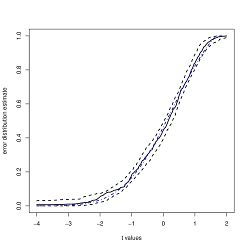
Figure 1. A plot of the error distribution function estimate (solid black curve) overlaid by approximate $95\%$ pointwise confidence intervals (dashed curves) and a plausible truncated normal error distribution (blue dot-dashed curve).

Our analysis considers three variables measured: the number of days before metastasis was detected (observed or censored), a censoring indicator and the patient’s age (in years). There are $286$ original data values, and about $63\%$ of the reported time lengths before metastasis had been detected were censored at large values (indicating a possible cure effect). The ages of the patients range between $26$ and $83$ years with a median age of $52$ years. The oldest patient with an uncensored response is $78$ years. Since there were only two (censored) observations for patients older than $80$, these cases were removed because the data was too sparse in this region to obtain good model estimates, and our analysis considers the remaining $284$ patients. We are interested in a nonparametric location-scale modelling of the log-transformed time length before detectable metastasis by the patient’s age that accounts for both the presence of censoring and an apparent presence of a cure effect.

We obtain from $a_{n}=C\hat{\sigma}_{X}n^{-1/4-\gamma}\log^{1/4+\gamma}(n)$, with $n=284$ and $\hat{\sigma}_{X}\approx 12.3$ years and choosing $C=9/8$ and $\gamma=1/28$, a bandwidth of $4.51$ years. This choice corresponds with our simulations from the previous section and corresponds with an appropriate choice for Theorem 2. The score function $J$ is chosen as in the previous section (a smooth approximation of a step function).

Pointwise confidence intervals for $\hat{\mathbb{F}}$ are built using a bootstrap as follows. We begin by sampling completely at random and with replacement from the ages of the patients (covariates). We then construct bootstrap uncured responses using model (1.1), where $m$ is replaced by the estimator $\hat{m}$, $s$ is replaced by the estimator $\hat{s}$ and the model errors are sampled independently from $\hat{\mathbb{F}}$ and then appropriately centered and scaled (see our discussion on identifiability in Section 2). In addition, a bootstrap cure indicator is independently generated from $\hat{\pi}$ for each selected age. When this indicator is equal to one the associated bootstrap uncured response value is replaced by $\infty$. Bootstrap censoring variables are then independently sampled from the local censoring distribution estimators at each selected age. The bootstrap responses are then obtained by taking the minimum between the resulting augmented uncured responses (that include $\infty$ as possible values) and the selected censoring variable. Whenever a response is not censored we set a bootstrap censoring indicator equal to one and zero otherwise. The bootstrap distribution of $\hat{\mathbb{F}}$ is simulated on $300$ replicate bootstrap datasets, and we obtain our confidence intervals using the approximate quantiles from the simulated bootstrap distribution.

The confidence intervals considered in this analysis have approximately $95\%$ coverage.

Figure 1 shows a plot of the error distribution function estimate, which appears to be truncated near $1.7$ and (comparing the solid black curve with the blue dot-dashed curve) this estimate appears to describe very well a (truncated) normal distribution. In conclusion, the estimator $\hat{\mathbb{F}}$ appears to be very promising for use in applications, and this estimator does not require a computationally costly bandwidth selection procedure to be effective.

4. Appendix

From the discussion in Section 2 we observed that (2.1) implies $\tau_{0}<\tau_{M}(x)$, $x\in[0,\,1]$. This means that we may view our cure model as a special case of right–censored response models. In the following result, we specify the asymptotic order of the estimators $\hat{M}$ and $\hat{M}^{1}$, which follows directly from Lemma 4.2 of Du and Akritas (2002).

Lemma 1.

Let Assumptions (A1) – (A4), (A5) (ii) and (iv) hold. Then

$$\sup_{x\in[0,\,1]}\sup_{-\infty<t\leq\tau_{0}}\big{|}\hat{M}(t\,|\,x)-M(t\,|\,x)\big{|}=O\big{(}(na_{n})^{-1/2}\log^{1/2}(n)\big{)},\qquad\text{a.s.},$$

and

$$\sup_{x\in[0,\,1]}\sup_{-\infty\leq t\leq\tau_{0}}\big{|}\hat{M}^{1}(t\,|\,x)-M^{1}(t\,|\,x)\big{|}=O\big{(}(na_{n})^{-1/2}\log^{1/2}(n)\big{)},\qquad\text{a.s.}$$

In addition, we can specify the asymptotic order for moduli of continuity for the estimators $\hat{M}$ and $\hat{M}^{1}$, which follows directly by applications of Lemma 4.4 of Du and Akritas (2002).

Lemma 2.

Let Assumptions (A1) – (A5) hold. Set $L=L_{1}+L_{2}$ and $b_{n}=O((na_{n})^{-1/2}\log^{1/2}(n))$. Then, almost surely,

$$\sup_{x\in[0,\,1]}\sup_{-\infty<s,t\leq\tau_{0}}\sup_{|L(t)-L(s)|\leq b_{n}}\big{|}\hat{M}(t\,|\,x)-M(t\,|\,x)-\hat{M}(s\,|\,x)+M(s\,|\,x)\big{|}=O\big{(}(na_{n})^{-3/4}\log^{3/4}(n)\big{)}$$

and, now with $L=L_{1}+L_{3}$,

$$\sup_{x\in[0,\,1]}\sup_{-\infty<s,t\leq\tau_{0}}\sup_{|L(t)-L(s)|\leq b_{n}}\big{|}\hat{M}^{1}(t\,|\,x)-M^{1}(t\,|\,x)-\hat{M}^{1}(s\,|\,x)+M^{1}(s\,|\,x)\big{|}=O\big{(}(na_{n})^{-3/4}\log^{3/4}(n)\big{)}.$$

In order to specify the asymptotic order and modulus of continuity for the hazard estimator $\hat{\Lambda}$, we need to state a technical result common for censored response models. Define

$$A_{n}(t\,|\,x)=\int_{-\infty}^{t}\frac{\hat{M}(s-\,|\,x)-M(s-\,|\,x)}{\{1-M(s-\,|\,x)\}^{2}}\big{\{}\hat{M}^{1}(ds\,|\,x)-M^{1}(ds\,|\,x)\big{\}}.$$

In the following result, we specify the asymptotic order of $A_{n}$. The proof of this result follows along the same lines as the proof of Proposition 4.1 of Du and Akritas (2002), and it is therefore omitted.

Proposition 4.

Let Assumptions (A1) – (A5) hold. Then

$$\sup_{x\in[0,\,1]}\sup_{-\infty<t\leq\tau_{0}}\big{|}A_{n}(t\,|\,x)\big{|}=O\big{(}(na_{n})^{-3/4}\log^{3/4}(n)\big{)},\qquad\text{a.s.}$$

With the results above we can state the asymptotic order and modulus of continuity for the hazard estimator $\hat{\Lambda}$.

Lemma 3.

Let Assumptions (A1) – (A5) hold. Then

$$\sup_{x\in[0,\,1]}\sup_{-\infty<t\leq\tau_{0}}\big{|}\hat{\Lambda}(t\,|\,x)-\Lambda(t\,|\,x)\big{|}=O\big{(}(na_{n})^{-1/2}\log^{1/2}(n)\big{)},\qquad\text{a.s.}$$

Set $L=L_{1}+L_{2}+L_{3}$ and $b_{n}=O((na_{n})^{-1/2}\log^{1/2}(n))$. Then

$$\sup_{x\in[0,\,1]}\sup_{-\infty<s,t\leq\tau_{0}}\sup_{|L(t)-L(s)|\leq b_{n}}\big{|}\hat{\Lambda}(t\,|\,x)-\Lambda(t\,|\,x)-\hat{\Lambda}(s\,|\,x)+\Lambda(s\,|\,x)\big{|}=O\big{(}(na_{n})^{-3/4}\log^{3/4}(n)\big{)},\qquad\text{a.s.}$$

Proof.

Beginning with the first assertion, we can write $\hat{\Lambda}(t\,|\,x)-\Lambda(t\,|\,x)=R_{1}(t\,|\,x)+R_{2}(t\,|\,x)+R_{3}(t\,|\,x)$, where

$$R_{1}(t\,|\,x)=\int_{-\infty}^{t}\frac{\hat{M}(s-\,|\,x)-M(s-\,|\,x)}{\{1-\hat{M}(s-\,|\,x)\}\{1-M(s-\,|\,x)\}}M^{1}(ds\,|\,x),$$

$$R_{2}(t\,|\,x)=\int_{-\infty}^{t}\frac{\hat{M}^{1}(ds\,|\,x)-M^{1}(ds\,|\,x)}{1-M(s-\,|\,x)}$$

and

$$R_{3}(t\,|\,x)=\int_{-\infty}^{t}\bigg{\{}\frac{\hat{M}(s-\,|\,x)-M(s-\,|\,x)}{\{1-\hat{M}(s-\,|\,x)\}\{1-M(s-\,|\,x)\}}\bigg{\}}\big{\{}\hat{M}^{1}(ds\,|\,x)-M^{1}(ds\,|\,x)\big{\}}.$$

Condition (2.1) implies that $M(t\,|\,x)<1$ for all $t\in(-\infty,\,\tau_{0}]$ and all $x\in[0,\,1]$. In addition, the assumptions of Lemma 1 are satisfied, which implies that $\sup_{x\in[0,\,1]}\sup_{-\infty<t\leq\tau_{0}}|\hat{M}(t\,|\,x)-M(t\,|\,x)|=O((na_{n})^{-1/2}\log^{1/2}(n))$, almost surely. Combining these results, it is easy to see that $\sup_{x\in[0,\,1]}\sup_{-\infty<t\leq\tau_{0}}|R_{1}(t\,|\,x)|=O((na_{n})^{-1/2}\log^{1/2}(n))$, almost surely. Using integration by parts, we can write $R_{2}(t\,|\,x)$ as

$$\frac{\hat{M}^{1}(t\,|\,x)-M^{1}(t\,|\,x)}{1-M(t-\,|\,x)}-\int_{-\infty}^{t}\frac{\hat{M}^{1}(s\,|\,x)-M^{1}(s\,|\,x)}{\{1-M(s-\,|\,x)\}^{2}}M(ds\,|\,x).$$

Similar to the first term, both of the terms in the display above have the order $O((na_{n})^{-1/2}\log^{1/2}(n))$, almost surely. The assumptions of Proposition 4 are satisfied. Combining the statement of this result with the uniform, strong consistency of $\hat{M}$ for $M$, it follows that $\sup_{x\in[0,\,1]}\sup_{-\infty<t\leq\tau_{0}}|R_{3}(t\,|\,x)|=O((na_{n})^{-3/4}\log^{3/4}(n))=o((na_{n})^{-1/2}\log^{1/2}(n))$, almost surely. This concludes the proof of the first assertion. The second assertion follows by similar arguments and is therefore omitted. ∎

With the results above on the cumulative hazard estimator $\hat{\Lambda}$, we can state the asymptotic orders of the strong, uniform consistency and modulus of continuity of the Beran estimator $\hat{Q}$. In addition, the uniform, strong i.i.d. representation of the Beran estimator $\hat{Q}$ is given.

Lemma 4 (properties of the Beran estimator $\hat{Q}$).

Let Assumptions (A1) – (A6) hold. Then

$$\sup_{x\in[0,\,1]}\sup_{-\infty<t\leq\tau_{0}}\big{|}\hat{Q}(t\,|\,x)-Q(t\,|\,x)\big{|}=O\big{(}(na_{n})^{-1/2}\log^{1/2}(n)\big{)},\qquad\text{a.s.}$$

Set $L=L_{1}+L_{2}+L_{3}$ and $b_{n}=O((na_{n})^{-1/2}\log^{1/2}(n))$. Then

$$\sup_{x\in[0,\,1]}\sup_{-\infty<s,t\leq\tau_{0}}\sup_{|L(t)-L(s)|\leq b_{n}}\big{|}\hat{Q}(t\,|\,x)-Q(t\,|\,x)-\hat{Q}(s\,|\,x)+Q(s\,|\,x)\big{|}=O\big{(}(na_{n})^{-3/4}\log^{3/4}(n)\big{)},\qquad\text{a.s.}$$

Finally, with $\zeta$ defined in Section 2.1,

$$\hat{Q}(t\,|\,x)-Q(t\,|\,x)=\frac{1-Q(t\,|\,x)}{g(x)na_{n}}\sum_{j=1}^{n}K\bigg{(}\frac{x-X_{j}}{a_{n}}\bigg{)}\zeta(x,Z_{j},\delta_{j},t)+R_{n}(t\,|\,x),$$

where $\sup_{x\in[0,\,1]}\sup_{t\in(-\infty,\,\tau_{0}]}|R_{n}(t\,|\,x)|=O((na_{n})^{-3/4}\log^{3/4}(n))$, almost surely.

Proof.

Write, as in the proof of Theorem 3.2 of Du and Akritas (2002),

$$\hat{Q}(t\,|\,x)-Q(t\,|\,x) =\{1-Q(t\,|\,x)\}\int_{-\infty}^{t}\frac{1-Q(t-\,|\,x)}{1-Q(t\,|\,x)}\,d\big{(}\hat{\Lambda}(t\,|\,x)-\Lambda(t\,|\,x)\big{)}$$

$$\quad+\{1-Q(t\,|\,x)\}\int_{-\infty}^{t}\frac{Q(t-\,|\,x)-\hat{Q}(t-\,|\,x)}{1-Q(t\,|\,x)}\,d\big{(}\hat{\Lambda}(t\,|\,x)-\Lambda(t\,|\,x)\big{)}.$$

Since $Y_{u}$ is a continuous random variable, it follows that $1-Q(t-\,|\,x)=1-Q(t\,|\,x)$ and the first term on the right-hand side in the display above is equal to $\{1-Q(t\,|\,x)\}\{\hat{\Lambda}(t\,|\,x)-\Lambda(t\,|\,x)\}$, which, by the first statement of Lemma 3, has the order $O((na_{n})^{-1/2}\log^{1/2}(n))$, almost surely, uniformly over $(t,x)\in(-\infty,\,\tau_{0}]\times[0,\,1]$. Following the arguments in the proof of Theorem 3.2 of Du and Akritas (2002), the second term has the order $O((na_{n})^{-3/4}\log^{3/4}(n))$, almost surely, uniformly over $(t,x)\in(-\infty,\,\tau_{0}]\times[0,\,1]$ (see the decomposition of $(\text{B})/S_{x}(t)$ into expressions $(5.5)$–$(5.8)$ in that article, where these expressions are shown to have the desired order). This completes the proof of the first assertion. The second assertion follows by a similar argument and is therefore omitted. Finally, the last assertion follows directly by an application of Theorem 3.2 of Du and Akritas (2002). ∎

López-Cheda et al. (2017) give the asymptotic order of strong consistency of $Z^{1}_{\text{max}}$ for $\tau_{0}$, which we restate here for convenience.

Lemma 5 (Lemma 5 of López-Cheda et al. (2017)).

Let Assumption (A7) hold. Then

$$n^{\alpha}\big{(}\tau_{0}-Z^{1}_{\text{max}}\big{)}=o(1),\quad\text{a.s.},\quad\alpha\in(0,\,1).$$

Note, for a sequence of bandwidths $a_{n}$ satisfying $a_{n}\to 0$, as $n\to\infty$, such that $na_{n}^{5}\log^{-1}(n)=O(1)$, it follows that

$$\tau_{0}-Z^{1}_{\text{max}}=o\big{(}(na_{n})^{-3/4}\log^{3/4}(n)\big{)},\qquad\text{a.s.}$$

We can now state the proof of Proposition 1 from Section 2.1.

Proof of Proposition 1.

Beginning with the first assertion, we can write $\hat{\pi}(x)-\pi(x)=R_{1}(x)+R_{2}(x)+R_{3}(x)$, where

$$R_{1}(x)=Q(\tau_{0}\,|\,x)-\hat{Q}(\tau_{0}\,|\,x),$$

$$R_{2}(x)=\hat{Q}(\tau_{0}\,|\,x)-Q(\tau_{0}\,|\,x)-\hat{Q}(Z^{1}_{\text{max}}\,|\,x)+Q(Z^{1}_{\text{max}}\,|\,x)$$

and

$$R_{3}(x)=Q(\tau_{0}\,|\,x)-Q(Z^{1}_{\text{max}}\,|\,x)$$

The assumptions of Lemma 4 are satisfied, and the first statement of this result implies that $\sup_{x\in[0,\,1]}|R_{1}(x)|=O((na_{n})^{-1/2}\log^{1/2}(n))$, almost surely. Since the assumptions of Lemma 5 are satisfied, we obtain the desired $\sup_{x\in[0,\,1]}|R_{2}(x)|=O((na_{n})^{-3/4}\log^{3/4}(n))$, almost surely, by combining the statement of Lemma 5 with the second statement of Lemma 4. Finally, combining the result of Lemma 5 with the fact that $Q$ has a bounded density shows that $\sup_{x\in[0,\,1]}|R_{3}(x)|=o((na_{n})^{-3/4}\log^{3/4}(n))$, almost surely. This finishes the proof of the first assertion. The second assertion follows from applying the third statement of Lemma 4 to $R_{1}(x)$. ∎

Next we give sketches of the proofs of Proposition 2 and Proposition 3 from Section 2.1 that follow along the same lines of arguments given in the proofs of Proposition 3, Proposition 6 and Proposition 7 of Akritas and Van Keilegom (2001).

Proof of Proposition 2.

We begin with proving the first assertion that $\|\hat{m}-m\|_{\infty}$ has the order $O((na_{n})^{-1/2}\log^{1/2}(n))$, almost surely, writing $\|\cdot\|_{\infty}$ for the supremum norm. Following the procedure in the proof of Proposition 3 from Akritas and Van Keilegom (2001), write $I(q)=\int_{0}^{q}J(p)\,dp$. We have that $\hat{m}(x)-m(x)$ is equal to

$$\int_{0}^{1}\hat{\xi}\big{(}\big{\{}1-\hat{\pi}(x)\big{\}}p\,\big{|}\,x\big{)}J(p)\,dp-\int_{0}^{1}\xi(\{1-\pi(x)\}p\,|\,x)J(p)\,dp$$

$$=\int_{0}^{1}\int_{-\infty}^{\tau_{0}}\mathbf{1}\bigg{[}\frac{\hat{Q}(t\,|\,x)}{1-\hat{\pi}(x)}\leq p\bigg{]}J(p)\,dt\,dp-\int_{0}^{1}\int_{-\infty}^{\tau_{0}}\mathbf{1}\bigg{[}\frac{Q(t\,|\,x)}{1-\pi(x)}\leq p\bigg{]}J(p)\,dt\,dp$$

(4.1) $$=\int_{-\infty}^{\tau_{0}}\bigg{\{}I\bigg{(}\frac{Q(t\,|\,x)}{1-\pi(x)}\bigg{)}-I\bigg{(}\frac{\hat{Q}(t\,|\,x)}{1-\hat{\pi}(x)}\bigg{)}\bigg{\}}\,dt,$$

where we have used that $I(1)=\int_{0}^{1}J(p)\,dp=1$ in the second equality. Since the score function $J$ is bounded, it follows that $I$ is Lipschitz continuous (with constant $\|J\|_{\infty}$) and $\|\hat{m}-m\|_{\infty}$ is bounded by

$$\bigg{[}\inf_{x\in[0,\,1]}\inf_{p_{l}\leq p\leq p_{u}}q\big{(}\xi(\{1-\pi(x)\}p\,|\,x)\,|\,x\big{)}\bigg{]}^{-1}\sup_{p_{l}\leq p\leq p_{u}}J(p)\sup_{x\in[0,\,1]}\sup_{-\infty<t\leq\tau_{0}}\bigg{|}\frac{\hat{Q}(t\,|\,x)}{1-\hat{\pi}(x)}-\frac{Q(t\,|\,x)}{1-\pi(x)}\bigg{|},$$

where the first two terms are finite. The last term is easily shown to be of order $O((na_{n})^{-1/2}\log^{1/2}(n))$, almost surely, using the first statement of Lemma 4 and the first statement of Proposition 1. This completes the proof of the first assertion.

Turning now to the second assertion, we can use the procedure in the proof of Proposition 6 of Akritas and Van Keilegom (2001); i.e. we can write $\hat{m}(x)-m(x)$ as

(4.2) $$\int_{-\infty}^{\tau_{0}}\bigg{\{}\frac{Q(t\,|\,x)}{1-\pi(x)}-\frac{\hat{Q}(t\,|\,x)}{1-\hat{\pi}(x)}\bigg{\}}J\big{(}Q_{u}(t\,|\,x)\big{)}\,dt+O\big{(}(na_{n})^{-1}\log(n)\big{)},\qquad\text{a.s.,}$$

using a Taylor expansion of $I$ in the right-hand side of (4.1) and the fact that $J^{\prime}$ is bounded. The difference term from (4.2) becomes

(4.3) $$\frac{Q(t\,|\,x)-\hat{Q}(t\,|\,x)}{1-\pi(x)}-Q_{u}(t\,|\,x)\frac{\hat{\pi}(x)-\pi(x)}{1-\pi(x)}+O\big{(}(na_{n})^{-1}\log(n)\big{)},\qquad\text{a.s.,}$$

where we have used that $Q(t\,|\,x)=\{1-\pi(x)\}Q_{u}(t\,|\,x)$. The third statement of Lemma 4 implies the first term in (4.3) is equal to

(4.4) $$-\frac{1-Q(t\,|\,x)}{1-\pi(x)}\frac{1}{g(x)na_{n}}\sum_{j=1}^{n}K\bigg{(}\frac{x-X_{j}}{a_{n}}\bigg{)}\zeta(x,Z_{j},\delta_{j},t)+O\big{(}(na_{n})^{-3/4}\log^{3/4}(n)\big{)}.$$

Applying the second statement of Proposition 1 shows the second term in (4.3) is equal to

(4.5) $$-\frac{\pi(x)}{1-\pi(x)}\frac{Q_{u}(t\,|\,x)}{g(x)na_{n}}\sum_{j=1}^{n}K\bigg{(}\frac{x-X_{j}}{a_{n}}\bigg{)}\zeta(x,Z_{j},\delta_{j},\tau_{0})+O\big{(}(na_{n})^{-3/4}\log^{3/4}(n)\big{)}.$$

Note, the order terms in the displays above hold uniformly over $(t,\,x)\in(-\infty,\,\tau_{0}]\times[0,\,1]$. The result then follows by combining (4.4) and (4.5) with the approximation (4.3) under the integral in (4.2). ∎

Proof of Proposition 3.

Beginning with the first assertion, write $\hat{v}(x)-v(x)$ as

(4.6) $$\int_{0}^{1}\hat{\xi}^{2}\big{(}\big{(}1-\hat{\pi}(x)\big{)}p\,|\,x\big{)}J(p)\,dp-\int_{0}^{1}\xi^{2}\big{(}(1-\pi(x))p\,|\,x\big{)}J(p)\,dp-\hat{m}^{2}(x)+m^{2}(x).$$

Since $\hat{m}^{2}(x)-m^{2}(x)=2m(x)\{\hat{m}(x)-m(x)\}+\{\hat{m}(x)-m(x)\}^{2}$, it follows from the first statement of Proposition 2 that $\|\hat{m}^{2}-m^{2}\|_{\infty}=O((na_{n})^{-1/2}\log^{1/2}(n))$, almost surely. With some technical effort, the difference of integrals in (4.6) can be shown to be equal to

$$\int_{0}^{\tau_{0}}\bigg{\{}I\bigg{(}\frac{Q(\sqrt{t}\,|\,x)}{1-\pi(x)}\bigg{)}-I\bigg{(}\frac{\hat{Q}(\sqrt{t}\,|\,x)}{1-\hat{\pi}(x)}\bigg{)}\bigg{\}}\,dt-\int_{0}^{\infty}\bigg{\{}I\bigg{(}\frac{Q(-\sqrt{t}\,|\,x)}{1-\pi(x)}\bigg{)}-I\bigg{(}\frac{\hat{Q}(-\sqrt{t}\,|\,x)}{1-\hat{\pi}(x)}\bigg{)}\bigg{\}}\,dt,$$

where $I(q)=\int_{0}^{q}J(p)\,dp$, $q\in[0,\,1]$. It therefore follows from similar lines of argument to those in the proof of Proposition 2 that the difference of integrals in (4.6) is of the order $O((na_{n})^{-1/2}\log^{1/2}(n))$, almost surely, uniformly in $x\in[0,\,1]$. Combining this statement with the statement $\|\hat{m}^{2}-m^{2}\|_{\infty}=O((na_{n})^{-1/2}\log^{1/2}(n))$, almost surely, from above, we can see that $\|\hat{v}-v\|_{\infty}=O((na_{n})^{-1/2}\log^{1/2}(n))$, almost surely. The first assertion then follows from the fact that

(4.7) $$\hat{s}(x)-s(x)+\frac{1}{2s(x)}\big{\{}\hat{s}(x)-s(x)\big{\}}^{2}=\frac{1}{2s(x)}\big{\{}\hat{v}(x)-v(x)\big{\}}.$$

To prove the second assertion, combine (4.6) with (4.7) to obtain the approximation for $\hat{s}(x)-s(x)$:

(4.8) $$\frac{1}{2s(x)}\bigg{\{}\int_{0}^{1}\hat{\xi}^{2}\big{(}\big{(}1-\hat{\pi}(x)\big{)}p\,|\,x\big{)}J(p)\,dp-\int_{0}^{1}\xi^{2}\big{(}(1-\pi(x))p\,|\,x\big{)}J(p)\,dp\bigg{\}}$$

$$\quad-\frac{m(x)}{s(x)}\big{\{}\hat{m}(x)-m(x)\big{\}}+O\big{(}(na_{n})^{-1}\log(n)\big{)},$$

where we have again used that $\hat{m}^{2}(x)-m^{2}(x)=2m(x)\{\hat{m}(x)-m(x)\}+\{\hat{m}(x)-m(x)\}^{2}$ and the order term holds almost surely, uniformly in $x\in[0,\,1]$. As above, with additional technical effort, the difference of integrals in (4.8) can be shown to be equal to

$$2\int_{-\infty}^{\tau_{0}}\bigg{\{}I\bigg{(}\frac{Q(y\,|\,x)}{1-\pi(x)}\bigg{)}-I\bigg{(}\frac{\hat{Q}(y\,|\,x)}{1-\hat{\pi}(x)}\bigg{)}\bigg{\}}y\,dy.$$

Therefore, one can then work with an expansion similar to (4.2) in the proof of Proposition 2 to derive an approximation of the first term in (4.8), i.e.

(4.9) $$\int_{-\infty}^{\tau_{0}}\bigg{\{}\frac{Q(y\,|\,x)-\hat{Q}(y\,|\,x)}{1-\pi(x)}-Q_{u}(y\,|\,x)\frac{\hat{\pi}(x)-\pi(x)}{1-\pi(x)}\bigg{\}}J\big{(}Q_{u}(y\,|\,x)\big{)}\frac{y}{s(x)}\,dy+O\big{(}(na_{n})^{-1}\log(n)\big{)},$$

where the order term holds almost surely, uniformly in $x\in[0,\,1]$. The result then follows by combining the approximations (4.4) and (4.5) from the proof of Proposition 2 with (4.9) for the first term in (4.8) and applying the second statement of Proposition 2 to the second term in (4.8). ∎

With the asymptotic properties of $\hat{Q}$, $\hat{\pi}$, $\hat{m}$ and $\hat{s}$ fully described, we can state the proof of our first main result: a strong uniform representation for the difference $\hat{\mathbb{F}}-F$.

Proof of Theorem 1.

We can write $\hat{\mathbb{F}}(t)-F(t)$ as

$$\frac{1}{n}\sum_{j=1}^{n}\frac{\hat{Q}(t\hat{s}(X_{j})+\hat{m}(X_{j})\,|\,X_{j})}{1-\hat{\pi}(X_{j})}-\frac{1}{n}\sum_{j=1}^{n}\frac{Q(ts(X_{j})+m(X_{j})\,|\,X_{j})}{1-\pi(X_{j})}$$

$$=\frac{1}{n}\sum_{j=1}^{n}\frac{\hat{Q}(ts(X_{j})+m(X_{j})\,|\,X_{j})-Q(ts(X_{j})+m(X_{j})\,|\,X_{j})}{1-\pi(X_{j})}$$

$$\quad+F(t)\frac{1}{n}\sum_{j=1}^{n}\frac{\hat{\pi}(X_{j})-\pi(X_{j})}{1-\pi(X_{j})}+f(t)\frac{1}{n}\sum_{j=1}^{n}\bigg{\{}t\frac{\hat{s}(X_{j})-s(X_{j})}{s(X_{j})}+\frac{\hat{m}(X_{j})-m(X_{j})}{s(X_{j})}\bigg{\}}$$

$$\quad+\frac{1}{n}\sum_{j=1}^{n}\frac{\hat{Q}(t\hat{s}(X_{j})+\hat{m}(X_{j})}{1-\pi(X_{j})}\frac{\{\hat{\pi}(X_{j})-\pi(X_{j})\}^{2}}{1-\hat{\pi}(X_{j})}$$

$$\quad+\frac{1}{n}\sum_{j=1}^{n}\bigg{\{}\Big{\{}\hat{Q}\big{(}t\hat{s}(X_{j})+\hat{m}(X_{j})\,\big{|}\,X_{j}\big{)}-Q\big{(}t\hat{s}(X_{j})+\hat{m}(X_{j})\,\big{|}\,X_{j}\big{)}$$

$$\qquad\phantom{+\frac{1}{n}\sum_{j=1}^{n}\bigg{\{}\Big{\{}}-\hat{Q}(ts(X_{j})+m(X_{j})\,|\,X_{j})+Q(ts(X_{j})+m(X_{j})\,|\,X_{j})\Big{\}}\Big{/}\Big{\{}1-\pi(X_{j})\Big{\}}\bigg{\}}$$

$$\qquad\phantom{+\frac{1}{n}\sum_{j=1}^{n}}\times\bigg{\{}\frac{\hat{\pi}(X_{j})-\pi(X_{j})}{1-\pi(X_{j})}\bigg{\}}$$

$$\quad+\frac{1}{n}\sum_{j=1}^{n}\frac{\hat{Q}(ts(X_{j})+m(X_{j})\,|\,X_{j})-Q(ts(X_{j})+m(X_{j})\,|\,X_{j})}{1-\pi(X_{j})}\frac{\hat{\pi}(X_{j})-\pi(X_{j})}{1-\pi(X_{j})}$$

$$\quad+\frac{1}{n}\sum_{j=1}^{n}\bigg{\{}F\bigg{(}t+t\frac{\hat{s}(X_{j})-s(X_{j})}{s(X_{j})}+\frac{\hat{m}(X_{j})-m(X_{j})}{s(X_{j})}\bigg{)}-F(t)\bigg{\}}\frac{\hat{\pi}(X_{j})-\pi(X_{j})}{1-\pi(X_{j})}$$

$$\quad+\frac{1}{n}\sum_{j=1}^{n}\Big{\{}\hat{Q}\big{(}t\hat{s}(X_{j})+\hat{m}(X_{j})\,\big{|}\,X_{j}\big{)}-Q\big{(}t\hat{s}(X_{j})+\hat{m}(X_{j})\,\big{|}\,X_{j}\big{)}$$

$$\qquad\phantom{+\frac{1}{n}\sum_{j=1}^{n}\Big{\{}}-\hat{Q}(ts(X_{j})+m(X_{j})\,|\,X_{j})+Q(ts(X_{j})+m(X_{j})\,|\,X_{j})\Big{\}}\Big{/}\Big{\{}1-\pi(X_{j})\Big{\}}$$

$$\quad+\frac{1}{n}\sum_{j=1}^{n}\bigg{\{}F\bigg{(}t+t\frac{\hat{s}(X_{j})-s(X_{j})}{s(X_{j})}+\frac{\hat{m}(X_{j})-m(X_{j})}{s(X_{j})}\bigg{)}-F(t)$$

$$\qquad\phantom{+\frac{1}{n}\sum_{j=1}^{n}\bigg{\{}}-f(t)\bigg{\{}t\frac{\hat{s}(X_{j})-s(X_{j})}{s(X_{j})}+\frac{\hat{m}(X_{j})-m(X_{j})}{s(X_{j})}\bigg{\}}\bigg{\}}.$$

We can therefore write

$$R_{4,n}(t)=\hat{\mathbb{F}}(t)-F(t)-E_{n}(t)=\sum_{i=1}^{10}D_{i,n}(t),$$

where $E_{n}(t)$ is defined in the statement of the theorem and

$$D_{1,n}(t)=\frac{1}{n}\sum_{j=1}^{n}\frac{\hat{Q}(t\hat{s}(X_{j})+\hat{m}(X_{j})\,|\,X_{j})}{1-\pi(X_{j})}\frac{\{\hat{\pi}(X_{j})-\pi(X_{j})\}^{2}}{1-\hat{\pi}(X_{j})},$$

$$D_{2,n}(t)=\frac{1}{n}\sum_{j=1}^{n} \bigg{\{}\Big{\{}\hat{Q}\big{(}t\hat{s}(X_{j})+\hat{m}(X_{j})\,\big{|}\,X_{j}\big{)}-Q\big{(}t\hat{s}(X_{j})+\hat{m}(X_{j})\,\big{|}\,X_{j}\big{)}$$

$$\phantom{\bigg{\{}\Big{\{}}\quad-\hat{Q}(ts(X_{j})+m(X_{j})\,|\,X_{j})+Q(ts(X_{j})+m(X_{j})\,|\,X_{j})\Big{\}}\Big{/}\Big{\{}1-\pi(X_{j})\Big{\}}\bigg{\}}$$

$$\quad\times\bigg{\{}\frac{\hat{\pi}(X_{j})-\pi(X_{j})}{1-\pi(X_{j})}\bigg{\}},$$

$$D_{3,n}(t)=\frac{1}{n}\sum_{j=1}^{n}\frac{\hat{Q}(ts(X_{j})+m(X_{j})\,|\,X_{j})-Q(ts(X_{j})+m(X_{j})\,|\,X_{j})}{1-\pi(X_{j})}\frac{\hat{\pi}(X_{j})-\pi(X_{j})}{1-\pi(X_{j})},$$

$$D_{4,n}(t)=\frac{1}{n}\sum_{j=1}^{n}\bigg{\{}F\bigg{(}t+t\frac{\hat{s}(X_{j})-s(X_{j})}{s(X_{j})}+\frac{\hat{m}(X_{j})-m(X_{j})}{s(X_{j})}\bigg{)}-F(t)\bigg{\}}\frac{\hat{\pi}(X_{j})-\pi(X_{j})}{1-\pi(X_{j})},$$

$$D_{5,n}(t)=\frac{1}{n}\sum_{j=1}^{n}\Big{\{} \hat{Q}\big{(}t\hat{s}(X_{j})+\hat{m}(X_{j})\,\big{|}\,X_{j}\big{)}-Q\big{(}t\hat{s}(X_{j})+\hat{m}(X_{j})\,\big{|}\,X_{j}\big{)}$$

$$\quad-\hat{Q}(ts(X_{j})+m(X_{j})\,|\,X_{j})+Q(ts(X_{j})+m(X_{j})\,|\,X_{j})\Big{\}}\Big{/}\Big{\{}1-\pi(X_{j})\Big{\}},$$

$$D_{6,n}(t)=\frac{1}{n}\sum_{j=1}^{n}\bigg{\{} F\bigg{(}t+t\frac{\hat{s}(X_{j})-s(X_{j})}{s(X_{j})}+\frac{\hat{m}(X_{j})-m(X_{j})}{s(X_{j})}\bigg{)}-F(t)$$

$$\quad-f(t)\bigg{\{}t\frac{\hat{s}(X_{j})-s(X_{j})}{s(X_{j})}+\frac{\hat{m}(X_{j})-m(X_{j})}{s(X_{j})}\bigg{\}}\bigg{\}},$$

$$D_{7,n}(t)=\frac{1}{n}\sum_{j=1}^{n}\frac{R_{n}(ts(X_{j})+m(X_{j})\,|\,X_{j})}{1-\pi(X_{j})},$$

where $R_{n}$ is given in the third statement of Lemma 4,

$$D_{8,n}(t)=F(t)\frac{1}{n}\sum_{j=1}^{n}\frac{R_{1,n}(X_{j})}{1-\pi(X_{j})},$$

where $R_{1,n}$ is given in the second statement of Proposition 1,

$$D_{9,n}(t)=f(t)\frac{1}{n}\sum_{j=1}^{n}\frac{R_{2,n}(X_{j})}{s(X_{j})},$$

where $R_{2,n}$ is given in the second statement of Proposition 2, and

$$D_{10,n}(t)=tf(t)\frac{1}{n}\sum_{j=1}^{n}\frac{R_{3,n}(X_{j})}{s(X_{j})},$$

where $R_{3,n}$ is given in the second statement of Proposition 3.

The assumptions of Proposition 1 are satisfied, and the first statement of this result gives $\|\hat{\pi}-\pi\|_{\infty}=O((na_{n})^{-1/2}\log^{1/2}(n))$, almost surely. Combining this statement with the facts that $\|\pi\|_{\infty}<1$ and that $|D_{1,n}(t)|$ is bounded by $[1-\|\pi\|_{\infty}]^{-1}[1-\|\hat{\pi}\|_{\infty}]^{-1}\|\hat{\pi}-\pi\|_{\infty}^{2}$ shows that $\|D_{1,n}\|_{\infty}$ is of the order $O((na_{n})^{-1}\log(n))=o((na_{n})^{-3/4}\log^{3/4}(n))$, almost surely.

We can see that $|D_{2,n}(t)|$ is bounded by

(4.10) $$\sup_{x\in[0,\,1]}\sup_{-\infty<t\leq\tau_{F}}\Big{|}\hat{Q}\big{(}t\hat{s}(x)+\hat{m}(x)\,\big{|}\,x\big{)}-Q\big{(}t\hat{s}(x)+\hat{m}(x)\,\big{|}\,x\big{)}$$

$$\phantom{\sup_{x\in[0,\,1]}\sup_{-\infty<t\leq\tau_{F}}\Big{|}}\quad-\hat{Q}(ts(x)+m(x)\,|\,x)+Q(ts(x)+m(x)\,|\,x)\Big{|}$$

$$\times\Big{[}1-\|\pi\|_{\infty}\Big{]}^{2}\sup_{x\in[0,\,1]}\Big{|}\hat{\pi}(x)-\pi(x)\Big{|},$$

and we have already used that $\|\pi\|_{\infty}<1$ and $\|\hat{\pi}-\pi\|_{\infty}=O((na_{n})^{-1/2}\log^{1/2}(n))$, almost surely. Hence, we only need to treat the first term in (4.10), which we do by using the modulus of continuity for the Beran estimator $\hat{Q}$ given in the second statement of Lemma 4. The assumptions of Lemma 4 are satisfied. However, in order to use the second statement of this result, we need to show the related result

$$\sup_{x\in[0,\,1]}\sup_{-\infty<t\leq\tau_{F}}\Big{|}L\big{(}t\hat{s}(x)+\hat{m}(x)\big{)}-L\big{(}ts(x)+m(x)\big{)}\Big{|}=O\big{(}(na_{n})^{-1/2}\log^{1/2}(n)\big{)},\qquad\text{a.s.}$$

This is equivalent to showing

(4.11) $$\sup_{x\in[0,\,1]}\sup_{-\infty<t\leq\tau_{0}}\bigg{|}L\bigg{(}t+t\frac{\hat{s}(x)-s(x)}{s(x)}+\frac{\hat{m}(x)-m(x)}{s(x)}\bigg{)}-L(t)\bigg{|}=O\big{(}(na_{n})^{-1/2}\log^{1/2}(n)\big{)},\qquad\text{a.s.}$$

To see that (4.11) holds, recall the sequences of real numbers $\{u_{n}\}_{n\geq 1}$ and $\{v_{n}\}_{n\geq 1}$ introduced in the discussion following (2.7). It follows that $|L(t+t(v_{n}-v)+u_{n}-u)-L(t)|$ is bounded by

(4.12) $$\big{|}u_{n}-u\big{|}\sup_{-\infty<t\leq\tau_{0}}\Big{|}L^{\prime}(t)\Big{|}+\big{|}v_{n}-v\big{|}\sup_{-\infty<t\leq\tau_{0}}\Big{|}tL^{\prime}(t)\Big{|}$$

$$+\sup_{-\infty<t\leq\tau_{0}}\Big{|}L\big{(}t+t(v_{n}-v)+u_{n}-u\big{)}-L\big{(}t+t(v_{n}-v)\big{)}-(u_{n}-u)L^{\prime}\big{(}t+t(v_{n}-v)\big{)}\Big{|}$$

$$+\sup_{-\infty<t\leq\tau_{0}}\Big{|}L\big{(}t+t(v_{n}-v)\big{)}-L(t)-(v_{n}-v)tL^{\prime}(t)\Big{|}.$$

The terms in the first line of (4.12) are easily seen to be of the order $O((v_{n}-v)+(u_{n}-u))$, as desired. The quantity inside the absolute brackets in the second line of the same display is equal to

(4.13) $$(u_{n}-u)\int_{0}^{1}\Big{\{}L^{\prime}\big{(}t+t(v_{n}-v)+p(u_{n}-u)\big{)}-L^{\prime}\big{(}t+t(v_{n}-v)\big{)}\Big{\}}\,dp.$$

We will now use (2.7) to show that (4.13) is of the order $O(|u_{n}-u|^{2})$. Let $-\infty<a<b\leq\tau_{0}$. It follows from the fact that $L$ is nondecreasing that $(1+a^{2})|L^{\prime}(b)-L^{\prime}(a)|$ is bounded by

$$\Big{|}\big{(}1+b^{2}\big{)}L^{\prime}(b)-\big{(}1+a^{2}\big{)}L^{\prime}(a)\Big{|}=\bigg{|}\int_{a}^{b}\,\big{(}1+w^{2}\big{)}L^{\prime\prime}(w)\,dw+2\int_{a}^{b}\,wL^{\prime}(w)\,dw\bigg{|}.$$

The triangle inequality in combination with (2.7) implies that the right-hand side of the display above is further bounded by

$$\int_{a}^{b}\,\big{(}1+w^{2}\big{)}\bigg{|}\frac{L^{\prime\prime}(w)}{L^{\prime}(w)}\bigg{|}\,L(dw)+2\sup_{-\infty<t\leq\tau_{0}}\big{|}tL^{\prime}(t)\big{|}\big{|}b-a\big{|}$$

$$\leq\Bigg{\{}\bigg{\{}\int_{0}^{1}\,\Big{(}1+\big{(}a+p(b-a)\big{)}^{2}\Big{)}\bigg{\{}\frac{L^{\prime\prime}(a+p(b-a))}{L^{\prime}(a+p(b-a))}\bigg{\}}^{2}L^{\prime}\big{(}a+p(b-a)\big{)}\,dp$$

$$\quad\phantom{\Bigg{\{}\bigg{\{}}\times\int_{0}^{1}\,\Big{(}1+\big{(}a+p(b-a)\big{)}^{2}\Big{)}L^{\prime}\big{(}a+p(b-a)\big{)}\,dp\bigg{\}}^{1/2}+2\sup_{-\infty<t\leq\tau_{0}}\Big{|}tL^{\prime}(t)\Big{|}\Bigg{\}}\big{|}b-a\big{|}$$

$$\leq\Bigg{\{}\bigg{\{}\int_{-\infty}^{\tau_{0}}\,\big{(}1+w^{2}\big{)}\bigg{\{}\frac{L^{\prime\prime}(w)}{L^{\prime}(w)}\bigg{\}}\,L(dw)\int_{-\infty}^{\tau_{0}}\,\big{(}1+w^{2}\big{)}\,L(dw)\bigg{\}}^{1/2}+2\sup_{-\infty<t\leq\tau_{0}}\Big{|}tL^{\prime}(t)\Big{|}\Bigg{\}}\big{|}b-a\big{|},$$

where the middle inequality follows from Hölder’s inequality and the final inequality follows by the facts that the integrands are nonnegative and $[a,\,b]\subset(-\infty,\,\tau_{0}]$. This means that we can find a constant $C>0$ such that

(4.14) $$\Big{|}L^{\prime}(b)-L^{\prime}(a)\Big{|}\leq C\frac{|b-a|}{1+a^{2}},\qquad-\infty<a,b\leq\tau_{0}.$$

Setting $a=\min\{t+t(v_{n}-v),\,t+t(v_{n}-v)+p(u_{n}-u)\}$ and $b=\max\{t+t(v_{n}-v),\,t+t(v_{n}-v)+p(u_{n}-u)\}$ in (4.14) implies that $|L^{\prime}(t+t(v_{n}-v)+p(u_{n}-u))-L^{\prime}(t+t(v_{n}-v))|$ is bounded by

(4.15) $$C\sup_{-\infty<t\leq\tau_{0}}\sup_{0\leq p\leq 1}\frac{|p|}{1+(\min\{t+t(v_{n}-v),\,t+t(v_{n}-v)+p(u_{n}-u)\})^{2}}\big{|}u_{n}-u\big{|}.$$

It follows for (4.13) to be of the order $O(|u_{n}-u|^{2})$, and, hence, the term in the second line of (4.12) is also of the order $O(|u_{n}-u|^{2})=o(|u_{n}-u|)$. A similar argument shows the term in the third line of (4.12) is of the order $O(|v_{n}-v|^{2})=o(|v_{n}-v|)$, where the fraction in (4.14) becomes $|p|t^{2}/(1+t^{2}(\min\{1,\,1+v_{n}-v\})^{2})$, which is bounded for all $n$ where $-1\neq v_{n}-v$. This shows the desired result

(4.16) $$\sup_{-\infty<t\leq\tau_{0}}\Big{|}L(t+t(v_{n}-v)+(u_{n}-u))-L(t)\Big{|}=O\big{(}|v_{n}-v|+|u_{n}-u|\big{)}.$$

Since the assumptions of Proposition 2 and Proposition 3 are satisfied, combining the first statements of these results with the fact that $s$ is bounded away from zero and (4.16) establishes the desired (4.11). We can therefore apply the second statement of Lemma 4 to see that the first term of (4.10) is of the order $O((na_{n})^{-3/4}\log^{3/4}(n))$. It then follows that $\|D_{2,n}\|_{\infty}$ is of the order $O((na_{n})^{-5/4}\log^{5/4}(n))=o((na_{n})^{-3/4}\log^{3/4}(n))$, almost surely.

We can use the first statements of Lemma 4 and Proposition 1 to treat $D_{3,n}(t)$, since this remainder term is bounded in absolute value by

$$\Big{[}1-\|\pi\|_{\infty}\Big{]}^{2}\sup_{x\in[0,\,1]}\sup_{-\infty<t\leq\tau_{0}}\big{|}\hat{Q}(t\,|\,x)-Q(t\,|\,x)\big{|}\sup_{x\in[0,\,1]}\big{|}\hat{\pi}(x)-\pi(x)\big{|}.$$

Therefore, $\|D_{3,n}\|_{\infty}$ is of the order $O((na_{n})^{-1}\log(n))=o((na_{n})^{-3/4}\log^{3/4}(n))$, almost surely.

Since $F$ satisfies (2.7), with $F$ in place of $L$, $f$ in place of $L^{\prime}$ and $f^{\prime}$ in place of $L^{\prime\prime}$, the same argument used to verify (4.11) can be used to show

$$\sup_{x\in[0,\,1]}\sup_{-\infty<t\leq\tau_{F}}\bigg{|}F\bigg{(}t+t\frac{\hat{s}(x)-s(x)}{s(x)}+\frac{\hat{m}(x)-m(x)}{s(x)}\bigg{)}-F(t)\bigg{|}=O\big{(}(na_{n})^{-1/2}\log^{1/2}(n)\big{)},\qquad\text{a.s.}$$

This fact combined with the result $\|\hat{\pi}-\pi\|_{\infty}=O((na_{n})^{-1/2}\log^{1/2}(n))$, almost surely, from the first statement of Proposition 1, and the fact that $|D_{4,n}(t)|$ is bounded by

$$\Big{[}1-\|\pi\|_{\infty}\Big{]}^{-1}\sup_{x\in[0,\,1]}\sup_{-\infty<t\leq\tau_{F}}\bigg{|}F\bigg{(}t+t\frac{\hat{s}(x)-s(x)}{s(x)}+\frac{\hat{m}(x)-m(x)}{s(x)}\bigg{)}-F(t)\bigg{|}\sup_{x\in[0,\,1]}\Big{|}\hat{\pi}(x)-\pi(x)\Big{|}$$

shows that $\|D_{4,n}\|_{\infty}$ is of the order $O((na_{n})^{-1}\log(n))=o((na_{n})^{-3/4}\log^{3/4}(n))$, almost surely.

Similar to the arguments for the remainder term $D_{2,n}(t)$, we can apply the second statement of Lemma 4 and the fact that $\|\pi\|_{\infty}<1$ to treat the remainder term $D_{5,n}(t)$, since $|D_{5,n}(t)|$ is bounded by $[1-\|\pi\|_{\infty}]^{-1}$ multiplied by

$$\sup_{x\in[0,\,1]}\sup_{-\infty<t\leq\tau_{F}}\Big{|}\hat{Q}\big{(}t\hat{s}(x)+\hat{m}(x)\,\big{|}\,x\big{)}-Q\big{(}t\hat{s}(x)+\hat{m}(x)\,\big{|}\,x\big{)}-\hat{Q}(ts(x)+m(x)\,|\,x)+Q(ts(x)+m(x)\,|\,x)\Big{|}.$$

Therefore, $\|D_{5,n}\|_{\infty}$ is of the order $O((na_{n})^{-3/4}\log^{3/4}(n))$, almost surely, because we have already shown that the quantity in the display above is $O((na_{n})^{-3/4}\log^{3/4}(n))$, almost surely, using the modulus of continuity of the Beran estimator $\hat{Q}$ given in the second statement of Lemma 4.

We can write the remainder term $D_{6,n}(t)$ as the sum

$$\frac{1}{n}\sum_{j=1}^{n}\bigg{\{}F\bigg{(}t+t\frac{\hat{s}(X_{j})-s(X_{j})}{s(X_{j})}+\frac{\hat{m}(X_{j})-m(X_{j})}{s(X_{j})}\bigg{)}-F\bigg{(}t+t\frac{\hat{s}(X_{j})-s(X_{j})}{s(X_{j})}\bigg{)}$$

$$\phantom{\frac{1}{n}\sum_{j=1}^{n}\bigg{\{}}\quad-f\bigg{(}t+t\frac{\hat{s}(X_{j})-s(X_{j})}{s(X_{j})}\bigg{)}\frac{\hat{m}(X_{j})-m(X_{j})}{s(X_{j})}\bigg{\}}$$

$$+\frac{1}{n}\sum_{j=1}^{n}\bigg{\{}F\bigg{(}t+t\frac{\hat{s}(X_{j})-s(X_{j})}{s(X_{j})}\bigg{)}-F(t)-tf(t)\frac{\hat{s}(X_{j})-s(X_{j})}{s(X_{j})}\bigg{\}}$$

$$+\frac{1}{n}\sum_{j=1}^{n}\bigg{\{}f\bigg{(}t+t\frac{\hat{s}(X_{j})-s(X_{j})}{s(X_{j})}\bigg{)}-f(t)\bigg{\}}\frac{\hat{m}(X_{j})-m(X_{j})}{s(X_{j})}.$$

Hence, $|D_{6,n}(t)|$ is bounded by the sum of the quantities

(4.17) $$\sup_{x\in[0,\,1]}\sup_{-\infty<t\leq\tau_{F}}\bigg{|} F\bigg{(}t+t\frac{\hat{s}(x)-s(x)}{s(x)}+\frac{\hat{m}(x)-m(x)}{s(x)}\bigg{)}-F\bigg{(}t+t\frac{\hat{s}(x)-s(x)}{s(x)}\bigg{)}$$

$$\quad-f\bigg{(}t+t\frac{\hat{s}(x)-s(x)}{s(x)}\bigg{)}\frac{\hat{m}(x)-m(x)}{s(x)}\bigg{|},$$

(4.18) $$\sup_{x\in[0,\,1]}\sup_{-\infty<t\leq\tau_{F}}\bigg{|}F\bigg{(}t+t\frac{\hat{s}(x)-s(x)}{s(x)}\bigg{)}-F(t)-tf(t)\frac{\hat{s}(x)-s(x)}{s(x)}\bigg{|}$$

and

(4.19) $$\bigg{[}\inf_{x\in[0,\,1]}s(x)\bigg{]}^{-1}\sup_{x\in[0,\,1]}\sup_{-\infty<t\leq\tau_{F}}\bigg{|}f\bigg{(}t+t\frac{\hat{s}(x)-s(x)}{s(x)}\bigg{)}-f(t)\bigg{|}\sup_{x\in[0,\,1]}\Big{|}\hat{m}(x)-m(x)\Big{|}.$$

Since $F$ satisfies (2.7), analogous arguments to those that are used to show the second and third terms of (4.12) are of the orders $O(|u_{n}-u|^{2})$ and $O(|v_{n}-v|^{2})$, respectively, combined with the first statements of Proposition 2 and Proposition 3 show the bounds (4.17) and (4.18) are both of the order $O((na_{n})^{-1}\log(n))=o((na_{n})^{-3/4}\log^{3/4}(n))$, almost surely. Also, a similar argument that is used to find the bound (4.15) combined with the first statement of Proposition 3 can be used to show the second term in (4.19) is of the order $O((na_{n})^{-1/2}\log^{1/2}(n))$, almost surely. The third term in (4.19) has the order $O((na_{n})^{-1/2}\log^{1/2}(n))$, almost surely, from the first statement of Proposition 2. Therefore, we can see that $\|D_{6,n}\|_{\infty}$ is of the order $O((na_{n})^{-1}\log(n))=o((na_{n})^{-3/4}\log^{3/4}(n))$, almost surely.

The assumptions of Lemma 4 are satisfied, and it follows from the third statement of this result that $\|R_{n}\|_{\infty}$ is of the order $O((na_{n})^{-3/4}\log^{3/4}(n))$, almost surely. It then follows that $\|D_{7,n}\|_{\infty}$ is also of the order $O((na_{n})^{-3/4}\log^{3/4}(n))$, almost surely, because $|D_{7,n}(t)|$ is bounded by $[1-\|\pi\|_{\infty}]^{-1}\|R_{n}\|_{\infty}$. Since $|D_{8}(t)|$ is bounded by $[1-\|\pi\|_{\infty}]^{-1}\|R_{1,n}\|_{\infty}$, it follows from the second statement of Proposition 1 for $\|D_{8}\|_{\infty}$ to be of the order $O((na_{n})^{-3/4}\log^{3/4}(n))$, almost surely. The second statement from Proposition 2 shows that $\|D_{9}\|_{\infty}$ is of the order $O((na_{n}^{-3/4}\log^{3/4}(n))$, almost surely, which follows from the fact that $|D_{9}(t)|$ is bounded by $\|f\|_{\infty}[\inf_{x\in[0,\,1]}s(x)]^{-1}\|R_{2,n}\|_{\infty}$. Similarly, the second statement of Proposition 3 shows that $\|D_{10,n}\|_{\infty}$ is of the order $O((na_{n})^{-3/4}\log^{3/4}(n))$, almost surely, which concludes the proof. ∎

Before we can prove of our second main result we need to state the asymptotic order of the mean of the process $\{E_{n}(t)\,:\,-\infty<t\leq\tau_{F}\}$ introduced in Theorem 1.

Lemma 6.

Under the conditions of Theorem 1 it follows that

$$\sup_{-\infty<t\leq\tau_{F}}\Big{|}E\big{[}E_{n}(t)\big{]}\Big{|}=O\big{(}a_{n}^{2}\big{)}.$$

Proof.

Recall from the statement of Theorem 1 that $E_{n}(t)=T_{n}(t)-f(t)\{U_{n}+tV_{n}\}-W_{n}(t)$. Hence, the assertion follows from showing $\|E[T_{n}]\|_{\infty}=O(a_{n}^{2})$, $|E[U_{n}]|=O(a_{n}^{2})$, $|E[V_{n}]|=O(a_{n}^{2})$ and $\|E[W_{n}]\|_{\infty}=O(a_{n}^{2})$. We will only show the result that $\|E[T_{n}]\|_{\infty}=O(a_{n}^{2})$ because the remaining statements follow by similar lines of argument.

Write

$$\frac{1-Q(ts(v+a_{n}w)+m(v+a_{n}w)\,|\,v+a_{m}w)}{1-\pi(v+a_{n}w)}-\frac{1-Q(ts(v)+m(v)\,|\,v)}{1-\pi(v)}$$

$$=a_{n}w\frac{\int_{0}^{1}\,\dot{\pi}(v+a_{n}wp)\,dp}{\{1-\pi(v+a_{n}w)\}\{1-\pi(v)\}},$$

where $\dot{\pi}$ is the first derivative of the function $\pi$ with respect to its argument. Additionally, write

(4.20) $$E\Big{[}\zeta\big{(}v+a_{n}w,Z,\delta,ts(v+a_{n}w)+m(v+a_{n}w)\big{)}\,\Big{|}\,X=v,\,X^{\prime}=v+a_{n}w\Big{]}$$

$$=-a_{n}w\int_{-\infty}^{ts(v)+m(v)}\,\frac{1}{1-M(s-\,|\,v)}\,\dot{M}^{1}(ds\,|\,v)-a_{n}w\int_{-\infty}^{ts(v)+m(v)}\,\frac{\dot{M}(s-\,|\,v)}{\{1-M(s-\,|\,v)\}^{2}}\,M^{1}(ds\,|\,v)$$

$$\quad+a_{n}w\int_{ts(v)+m(v)}^{ts(v+a_{n}w)+m(v+a_{n}w)}\,\frac{\int_{0}^{1}\,\dot{M}(s-\,|\,v+a_{n}wp)\,dp}{\{1-M(s-\,|\,v+a_{n}w)\}\{1-M(s-\,|\,v)\}}\,M^{1}(ds\,|\,v)$$

$$\quad-a_{n}w\int_{ts(v)+m(v)}^{ts(v+a_{n}w)+m(v+a_{n}w)}\,\frac{\int_{0}^{1}\,\dot{M}(s-\,|\,v+a_{n}wp)\,dp}{\{1-M(s-\,|\,v+a_{n}w)\}^{2}}\,M^{1}(ds\,|\,v+a_{n}w)$$

$$\quad-a_{n}w\int_{ts(v)+m(v)}^{ts(v+a_{n}w)+m(v+a_{n}w)}\,\frac{\int_{0}^{1}\,\dot{M}(s-\,|\,v+a_{n}wp)\,dp}{\{1-M(s-\,|\,v+a_{n}w)\}\{1-M(s-\,|\,v)\}}\,M^{1}(ds\,|\,v+a_{n}w)$$

$$\quad-a_{n}w\int_{0}^{1}\,\bigg{\{}\int_{ts(v)+m(v)}^{ts(v+a_{n}w)+m(v+a_{n}w)}\,\frac{1}{1-M(s-\,|\,v)}\,\dot{M}^{1}(ds\,|\,v+a_{n}wq)\bigg{\}}\,dq$$

$$\quad-a_{n}^{2}w^{2}\int_{-\infty}^{ts(v)+m(v)}\,\frac{\int_{0}^{1}\,p\{\int_{0}^{1}\,\ddot{M}(s-\,|\,v+a_{n}wpq)\,dq\}\,dp}{\{1-M(s-\,|\,v)\}^{2}}\,M^{1}(ds\,|\,v)$$

$$\quad-a_{n}^{2}w^{2}\int_{-\infty}^{ts(v)+m(v)}\,\frac{\{\int_{0}^{1}\,\dot{M}(s-\,|\,v+a_{n}wp)\,dp\}^{2}}{\{1-M(s-\,|\,v+a_{n}w)\}\{1-M(s-\,|\,v)\}^{2}}\,M^{1}(ds\,|\,v)$$

$$\quad-a_{n}^{2}w^{2}\int_{-\infty}^{ts(v)+m(v)}\,\frac{\{\int_{0}^{1}\,\dot{M}(s-\,|\,v+a_{n}wp)\,dp\}^{2}}{\{1-M(s-\,|\,v+a_{n}w)\}^{2}\{1-M(s-\,|\,v)\}}\,M^{1}(ds\,|\,v)$$

$$\quad-a_{n}^{2}w^{2}\int_{0}^{1}\,\bigg{\{}\int_{-\infty}^{ts(v)+m(v)}\,\frac{\int_{0}^{1}\,\dot{M}(s-\,|\,v+a_{n}wp)\,dp}{\{1-M(s-\,|\,v+a_{n}w)\}^{2}}\,\dot{M}^{1}(ds\,|\,v+a_{n}wq)\bigg{\}}\,dq$$

$$\quad-a_{n}^{2}w^{2}\int_{0}^{1}\bigg{\{}\int_{-\infty}^{ts(v)+m(v)}\,\frac{\int_{0}^{1}\,\dot{M}(s-\,|\,v+a_{n}wp)\,dp}{\{1-M(s-\,|\,v+a_{n}w)\}\{1-M(s-\,|\,v)\}}\,\dot{M}^{1}(ds\,|\,v+a_{n}wq)\bigg{\}}\,dq$$

$$\quad-a_{n}^{2}w^{2}\int_{0}^{1}\,p\bigg{\{}\int_{0}^{1}\,\bigg{\{}\int_{-\infty}^{ts(v)+m(v)}\,\frac{1}{1-M(s-\,|\,v)}\,\ddot{M}^{1}(ds\,|\,v+a_{n}wpq)\bigg{\}}\,dq\bigg{\}}\,dp.$$

Here $\ddot{M}$ is the second partial derivative of $M$ with respect to $x$ and $\ddot{M}^{1}$ is the second partial derivative of $M^{1}$ with respect to $x$. For large enough $n$, $E[T_{n}(t)]$ is equal to

(4.21) $$\int_{0}^{1}\bigg{\{}\int_{-1}^{1}\,E\Big{[}\zeta\big{(}v+a_{n}w,Z,\delta,ts(v+a_{n}w)+m(v+a_{n}w)\big{)}\,\Big{|}\,X=v,\,X^{\prime}=v+a_{n}w\Big{]}K(w)\,dw\bigg{\}}$$

$$\phantom{\int_{0}^{1}}\quad\times\frac{1-Q(ts(v)+m(v)\,|\,v)}{1-\pi(v)}\,dv$$

$$+a_{n}\int_{0}^{1}\bigg{\{}\int_{-1}^{1}\,E\Big{[}\zeta\big{(}v+a_{n}w,Z,\delta,ts(v+a_{n}w)+m(v+a_{n}w)\big{)}\,\Big{|}\,X=v,\,X^{\prime}=v+a_{n}w\Big{]}$$

$$\phantom{+a_{n}\int_{0}^{1}\bigg{\{}\int_{-1}^{1}\,}\quad\times\frac{\int_{0}^{1}\,\dot{\pi}(v+a_{n}ws)\,ds}{\{1-\pi(v+a_{n}w)\}\{1-\pi(v)\}}wK(w)\,dw\bigg{\}}\,dv.$$

Since the first two terms on the right-hand side of (4.20) depend only on $w$ multiplied by a quantity not depending on $w$, the kernel function $K$ having mean zero implies the associated terms in (4.21) are equal to zero, while the remaining terms in the right-hand side of (4.20) are easily shown to be of the order $O(a_{n}^{2})$. The assertion then follows by combining the right-hand side of (4.20) with expression (4.21), and observing the remaining nonzero terms are all of the order $O(a_{n}^{2})$ or $o(a_{n}^{2})$. ∎

To continue we will introduce some notation. Write $\mathcal{H}$ for a class of measurable functions and let $\rho$ be a pseudometric for $\mathcal{H}$. As is in Definition 2.1.5 of van der Vaart and Wellner (1996), we will call $N(\epsilon,\mathcal{H},\rho)$ the covering number of $\mathcal{H}$, which is the minimum number of balls $\{g\,:\,\rho(g,h)<\epsilon\}$ of radius $\epsilon$ that is required to cover $\mathcal{H}$. Note that the centers of the balls need not belong to $\mathcal{H}$, but are required to have finite length under $\rho$. We will call the logarithm of the covering number the entropy. Also as in Definition 2.1.6 of van der Vaart and Wellner (1996), when given two functions satisfying $h_{l}\leq h_{u}$ we will call the collection of functions from $\mathcal{H}$ satisfying $h_{l}\leq h\leq h_{u}$ a bracket, and an $\epsilon$-bracket when the length of $h_{u}-h_{l}$ under $\rho$ is smaller than $\epsilon$. We will then call the minimum number of $\epsilon$-brackets required to cover $\mathcal{H}$ the bracketing number of $\mathcal{H}$, and write $N_{[\,]}(\epsilon,\mathcal{H},\rho)$. As in the definition of the covering number, the bracketing functions $h_{l}\leq h_{u}$ need not belong to $\mathcal{H}$ but are required to have finite lengths under $\rho$.

It is common to let the pseudometric $\rho$ be a scaled $L_{q}(P)$–metric for some $q\geq 1$ ($\rho_{L_{q}(P)}(h,g)\propto[\,\int\,|h-g|^{q}\,dP\,]^{1/q}$) or a scaled supremum metric (see $\|\cdot\|_{\infty}$ introduced at the beginning of Section 2). A function $H$ such that $|h|\leq H$ for every $h\in\mathcal{H}$ is called an envelope function for $\mathcal{H}$, and this function is useful for scaling the pseudometric $\rho$. When $\int\,H^{q}\,dP<\infty$ it is helpful to think of $\mathcal{H}$ as a subset of the class $\mathcal{L}_{q}(P)$, writing $\mathcal{L}_{q}(P)$ for the class of measurable functions with finite length under the $L_{q}(P)$–metric. Covering numbers and bracketing numbers are very helpful in understanding asymptotic properties of the process $\{n^{-1/2}\{\hat{\mathbb{F}}(t)-F(t)\}\,:\,-\infty<t\leq\tau_{F}\}$, which depends on the index set $-\infty<t\leq\tau_{F}$ and a bandwidth sequence $\{a_{n}\}_{n\geq 1}$. We conclude this section with the proof of our second main result: the weak convergence of $n^{1/2}\{\hat{\mathbb{F}}-F\}$.

Proof of Theorem 2.

The conditions of Theorem 1 are satisfied with $(na_{n})^{-3/4}\log^{3/4}(n)=o(n^{-1/2})$, and we can write $\hat{\mathbb{F}}(t)-F(t)=E_{n}(t)+o_{P}(n^{-1/2})$, $-\infty<t\leq\tau_{F}$, where the process $E_{n}(t)=T_{n}(t)-f(t)\{U_{n}+tV_{n}\}-W_{n}(t)$ depends on the random quantities $T_{n}(t)$, $U_{n}$, $V_{n}$ and $W_{n}(t)$ given in Theorem 1. Since $E_{n}(t)$ is not centered and the conditions of Lemma 6 are satisfied with $a_{n}^{2}=o(n^{-1/2})$, we center the process $E_{n}(t)$ to obtain $\hat{\mathbb{F}}(t)-F(t)=E_{n}(t)-E[E_{n}(t)]+o_{P}(n^{-1/2})=T_{n}(t)-E[T_{n}(t)]-f(t)\{U_{n}-E[U_{n}]+t\{V_{n}-E[V_{n}]\}\}-\{W_{n}(t)-E[W_{n}(t)]\}+o_{P}(n^{-1/2})$. The assertion follows if each of $T_{n}(t)-E[T_{n}(t)]$, $U_{n}-E[U_{n}]$, $V_{n}-E[V_{n}]$ and $W_{n}(t)-E[W_{n}(t)]$ are asymptotically linear and satisfy appropriate central limit theorems. We will prove only that $T_{n}(t)-E[T_{n}(t)]$ is asymptotically linear, uniformly in $-\infty<t\leq\tau_{F}$, and satisfies a functional central limit theorem. The remaining statements can be shown using similar and easier arguments that have been omitted for brevity.

We will now introduce some notation. As in Pakes and Pollard (1989), we will call a class of functions $\mathcal{H}$ a Euclidean class with envelope function $H$ (with respect to the $L_{q}(P)$–metric) when there are constants $C_{1},C_{2}>0$ such that the covering numbers $N(\epsilon,\mathcal{H},L_{q}(P))$ satisfy

$$N\big{(}\epsilon,\mathcal{H},L_{q}(P)\big{)}\leq C_{2}\epsilon^{-C_{1}},\quad 0<\epsilon\leq 1.$$

The constants $C_{1}$ and $C_{2}$ cannot depend on $P$. Note, Sherman (1994) requires that the envelope $H$ satisfies $\int\,H^{2}\,dP<\infty$. This condition is always satisfied for uniformly bounded $H$, and in this case we do not mention the distribution $P$.

To show that $T_{n}(t)-E[T_{n}(t)]$ is asymptotically linear, we will apply results from Sherman (1994), who studies weak convergence of degenerate $U$-processes of order $k\geq 1$. Using the Hoeffding decomposition of a $U$-process, this author is able to obtain several useful results concerning tightness properties of these processes. Corollary 7 of Sherman (1994) states that $k$-th order $U$-processes indexed by a Euclidean class of mean zero functions is asymptotically tight at the root-$n$ rate, i.e. $O_{P}(n^{-1/2})$.

The class of mean zero functions associated to $T_{n}(t)-E[T_{n}(t)]$ is $\mathcal{T}=\mathcal{T}_{1}-\mathcal{T}_{2}$ with $\mathcal{T}_{1}$ equal to

$$\bigg{\{}((X,Z,\delta),\,(X^{\prime},Z^{\prime},\delta^{\prime}))\mapsto \frac{1}{a}K\bigg{(}\frac{X-X^{\prime}}{a}\bigg{)}\frac{1-Q(ts(X)+m(X)\,|\,X)}{1-\pi(X)}\frac{\zeta(X,Z^{\prime},\delta^{\prime},ts(X)+m(X))}{g(X)}$$

$$\quad\,:\,0<a<1,\,-\infty<t\leq\tau_{F}\bigg{\}}$$

and $\mathcal{T}_{2}=\{((X,Z,\delta),\,(X^{\prime},Z^{\prime},\delta^{\prime}))\mapsto E[f_{a,t}((X,Z,\delta),(X^{\prime},Z^{\prime},\delta^{\prime}))]\,:\,f_{a,t}\in\mathcal{T}_{1}\}$. We can see that the amount of entropy residing in the class $\mathcal{T}_{2}$ is proportional to that residing in the class $\mathcal{T}_{1}$, which can be decomposed into the product of three classes:

$$\mathcal{K}=\bigg{\{}U=X-X^{\prime}\mapsto\frac{1}{a}K\bigg{(}\frac{U}{a}\bigg{)}\,:\,0<a<1\bigg{\}},$$

$$\mathcal{S} =\bigg{\{}X\mapsto\frac{1-Q(ts(X)+m(X)\,|\,X)}{1-\pi(X)}\,:\,-\infty<t\leq\tau_{F}\bigg{\}}$$

$$=\bigg{\{}X\mapsto\frac{\pi(X)}{1-\pi(X)}+1-F(t)\,:\,-\infty<t\leq\tau_{F}\bigg{\}}$$

and

$$\mathcal{Z}=\bigg{\{}((X,Z,\delta),(X^{\prime},Z^{\prime},\delta^{\prime}))\mapsto\frac{\zeta(X,Z^{\prime},\delta^{\prime},ts(X)+m(X))}{g(X)}\,:\,-\infty<t\leq\tau_{F}\bigg{\}}.$$

We can conclude that $\mathcal{T}$ is a Euclidean class when we have shown that $\mathcal{K}$, $\mathcal{S}$ and $\mathcal{Z}$ are each Euclidean classes. The class $\mathcal{K}$ is Euclidean by Lemma 22 of Nolan and Pollard (1987) with constant envelope $\|K\|_{\infty}$.

We will now show that the class $\mathcal{S}$ is Euclidean. Let $\epsilon>0$. Since $F$ is a continuous distribution function, we can partition the (infinite length) interval $[-\infty,\,\tau_{F}]$ into segments $[t_{i},\,t_{i+1}]$ satisfying $\max_{i}|F(t_{i+1})-F(t_{i})|\leq\epsilon$ by taking an $\epsilon$-net of $[0,\,1]$, consisting of $O(\epsilon^{-1})$ many links, and using the quantile $F^{-1}$ to define the corresponding points $t_{i}$, $i=1,\ldots,O(\epsilon^{-1})$, that partition the interval $[-\infty,\,\tau_{F}]$. Monotonicity of $F$ motivates the following brackets for a function from $\mathcal{S}$:

$$\frac{\pi(X)}{1-\pi(X)}+1-F(t_{i+1})\leq\frac{\pi(X)}{1-\pi(X)}+1-F(t)\leq\frac{\pi(X)}{1-\pi(X)}+1-F(t_{i}),\qquad t_{i}\leq t\leq t_{i+1}.$$

Working with the supremum metric, we find the maximal length of our brackets is $\max_{i}|F(t_{i+1})-F(t_{i})|\leq\epsilon$ as desired. Therefore, the number of brackets required to cover $\mathcal{S}$ with respect to the supremum metric, $N_{[\,]}(\epsilon,\mathcal{S},\|\cdot\|_{\infty})$, is $O(\epsilon^{-1})$. Hence, there is a constant $C>0$ such that $N_{[\,]}(\epsilon,\mathcal{S},\|\cdot\|_{\infty})\leq C\epsilon^{-1}$, and it follows that $\mathcal{S}$ is Euclidean with constant envelope $\|\pi\|_{\infty}/(1-\|\pi\|_{\infty})+1$.

To show that the class $\mathcal{Z}$ is Euclidean, we write $\mathcal{Z}=\mathcal{Z}_{1}-\mathcal{Z}_{2}$ as a difference of two classes, where

$$\mathcal{Z}_{1}=\bigg{\{}\big{(}(X,Z,\delta),\,(X^{\prime},Z^{\prime},\delta^{\prime})\big{)}\mapsto\frac{\delta^{\prime}\mathbf{1}[Z^{\prime}\leq ts(X)+m(X)]}{\{1-M(Z^{\prime}-\,|\,X)\}g(X)}\,:\,-\infty<t\leq\tau_{F}\bigg{\}}$$

and $\mathcal{Z}_{2}$ is equal to

$$\bigg{\{}\big{(}(X,Z,\delta),\,(X^{\prime},Z^{\prime},\delta^{\prime})\big{)}\mapsto\int_{-\infty}^{ts(X)+m(X)}\,\frac{\mathbf{1}[Z^{\prime}>u]}{\{1-M(Z^{\prime}-\,|\,X)\}^{2}g(X)}\,M^{1}(du\,|\,X)\,:\,-\infty<t\leq\tau_{F}\bigg{\}}.$$

We can therefore conclude that $\mathcal{Z}$ is a Euclidean class when we have shown that both $\mathcal{Z}_{1}$ and $\mathcal{Z}_{2}$ are each Euclidean classes.

Letting $\epsilon>0$, as before with the class $\mathcal{S}$, we can partition $[-\infty,\,\tau_{F}]$ into segments using points $t_{i}$, $i=1,\ldots,O(\epsilon^{-2})$, such that

$$\max_{i}\sup_{0\leq x\leq 1}\Big{|}M^{1}\big{(}t_{i+1}s(x)+m(x)\,|\,x\big{)}-M^{1}\big{(}t_{i}s(x)+m(x)\,|\,x\big{)}\Big{|}\leq\Big{[}1-\|M\|_{\infty}\Big{]}^{2}\bigg{[}\inf_{0\leq x\leq 1}g(x)\bigg{]}^{2}\epsilon^{2}.$$

Also similar to the above arguments, monotonicity of the indicator function motivates the following brackets for a function from $\mathcal{Z}_{1}$:

$$\frac{\delta^{\prime}\mathbf{1}[Z^{\prime}\leq t_{i}s(X)+m(X)]}{\{1-M(Z^{\prime}-\,|\,X)\}g(X)}\leq\frac{\delta^{\prime}\mathbf{1}[Z^{\prime}\leq ts(X)+m(X)]}{\{1-M(Z^{\prime}-\,|\,X)\}g(X)}\leq\frac{\delta^{\prime}\mathbf{1}[Z^{\prime}\leq t_{i+1}s(X)+m(X)]}{\{1-M(Z^{\prime}-\,|\,X)\}g(X)},$$

when $t_{i}\leq t\leq t_{i+1}$. The squared length of the proposed brackets in the $L_{2}(P\otimes P)$–metric satisfies

$$E\Bigg{[}\bigg{\{}\frac{\delta^{\prime}\mathbf{1}[Z^{\prime}\leq t_{i+1}s(X)+m(X)]}{\{1-M(Z^{\prime}-\,|\,X)\}g(X)}-\frac{\delta^{\prime}\mathbf{1}[Z^{\prime}\leq t_{i}s(X)+m(X)]}{\{1-M(Z^{\prime}\,|\,X)\}g(X)}\bigg{\}}^{2}\Bigg{]}$$

$$\leq\Big{[}1-\|M\|_{\infty}\Big{]}^{-2}\bigg{[}\inf_{0\leq x\leq 1}g(x)\bigg{]}^{-2}\sup_{0\leq x\leq 1}\Big{|}M^{1}\big{(}t_{i+1}s(x)+m(x)\,|\,x\big{)}-M^{1}\big{(}t_{i}s(x)+m(x)\,|\,x\big{)}\Big{|}$$

$$\leq\epsilon^{2},\qquad i=1,\ldots,O\big{(}\epsilon^{-2}\big{)}.$$

Since $\mathcal{Z}_{1}$ has the constant envelope $(1-\|M\|_{\infty})^{-1}[\inf_{0\leq x\leq 1}g(x)]^{-1}$, it then follows for the number of brackets required to cover $\mathcal{Z}_{1}$, $N_{[\,]}(\epsilon,\mathcal{Z}_{1},L_{2}(P\otimes P))$, is $O(\epsilon^{-2})$. Hence, $\mathcal{Z}_{1}$ is Euclidean. The class $\mathcal{Z}_{2}$ can also be shown to be Euclidean by a similar (and easier) argument, which is omitted. We conclude that the class $\mathcal{Z}$ is Euclidean as desired.

Therefore, $\mathcal{T}$ is Euclidean and the requirements for Corollary 7 of Sherman (1994) are satisfied. We can decompose $T_{n}(t)$ into

$$\chi_{n}(t)=\frac{1}{n(n-1)a_{n}}\sum_{j\neq k}K\bigg{(}\frac{X_{j}-X_{k}}{a_{n}}\bigg{)}\frac{1-Q(ts(X_{j})+m(X_{j})\,|\,X_{j})}{1-\pi(X_{j})}\frac{\zeta(X_{j},Z_{j},\delta_{j},ts(X_{j})+m(X_{j}))}{g(X_{j})},$$

and a remainder term $T_{n}(t)-\chi_{n}(t)$ that is equal to

$$\frac{1}{na_{n}}\frac{1}{n}\sum_{j=1}^{n}K(0)\frac{1-Q(ts(X_{j})+m(X_{j})\,|\,X_{j})}{1-\pi(X_{j})}\frac{\zeta(X_{j},Z_{j},\delta_{j},ts(X_{j})+m(X_{j}))}{g(X_{j})}-\frac{1}{n}\chi_{n}(t),$$

with $-\infty<t\leq\tau_{F}$. Therefore, up to symmetry in the kernel, $\chi_{n}(t)-E[\chi_{n}(t)]$ is a $2^{\text{nd}}$-order degenerate $U$-process. Note, from the discussion on page 439 of Sherman (1994), the kernel function characterizing the process $\chi_{n}(t)-E[\chi_{n}(t)]$ need not be symmetric in its arguments in order for the conclusions from Sherman (1994) to hold because the corresponding $U$-process is given by symmetrizing the kernel function. We can therefore apply Corollary 7 of Sherman (1994) to see that both $\|\chi_{n}-E[\chi_{n}]\|_{\infty}=O_{P}(n^{-1/2})$ and the remainder satisfies $\|T_{n}-E[T_{n}]-\chi_{n}+E[\chi_{n}]\|_{\infty}=o_{P}(n^{-1/2})$. However, $\chi_{n}(t)-E[\chi_{n}(t)]$ is not asymptotically linear.

To continue, approximate $\chi_{n}(t)-E[\chi_{n}(t)]$ by its Hájek projection. For large enough $n$, a function $\eta_{a,t}\in\mathcal{T}_{1}$ has the Hájek projection $h_{a,t}=h_{1,a,t}+h_{2,a,t}$, where

$$h_{1,a,t}(X_{j},Z_{j},\delta_{j}) =E\big{[}\eta_{a,t}((X,Z,\delta),(X_{j},Z_{j},\delta_{j}))\,|\,(X_{j},Z_{j},\delta_{j})\big{]}$$

$$=\int_{-1}^{1}\,\frac{1-Q(ts(X_{j}+au)+m(X_{j}+au)\,|\,X_{j}+au)}{1-\pi(X_{j}+au)}$$

$$\quad\phantom{=\int_{-1}^{1}\,}\times\zeta(X_{j}+au,Z_{j},\delta_{j},ts(X_{j}+au)+m(X_{j}+au))K(u)\,du$$

and

$$h_{2,a,t}(X_{j},Z_{j},\delta_{j}) =E\big{[}\eta_{a,t}((X_{j},Z_{j},\delta_{j}),(X,Z,\delta))\,|\,(X_{j},Z_{j},\delta_{j})\big{]}$$

$$=\frac{1-Q(ts(X_{j})+m(X_{j})\,|\,X_{j})}{1-\pi(X_{j})}$$

$$\quad\times\int_{-1}^{1}\,E\big{[}\zeta(X_{j},Z,\delta,ts(X_{j})+m(X_{j}))\,|\,X_{j},\,X=X_{j}+au\big{]}\frac{g(X_{j}+au)}{g(X_{j})}K(u)\,du.$$

The Hájek projection of $\chi_{n}(t)-E[\chi_{n}(t)]$ is then given by $n^{-1}\sum_{j=1}^{n}h_{a_{n},t}(X_{j},Z_{j},\delta_{j})-E[h_{a_{n},t}(X,Z,\delta)]$, where the bandwidth parameter $a_{n}$ appears in place of $a$.

From Lemma 6 of Sherman (1994), it follows that the class of Hájek projections, i.e.

$$\bigg{\{}(X,Z,\delta)\mapsto h_{a,t}(X,Z,\delta)-E\big{[}h_{a,t}(X,Z,\delta)\big{]}\,:\,0\leq a<1,\,-\infty<t\leq\tau_{F}\bigg{\}},$$

is Euclidean from the fact that $\mathcal{T}$ is Euclidean. We can therefore apply Corollary 4 (ii) of Sherman (1994) to see that

$$\sup_{t\in\mathbb{R}}\Big{|}\chi_{n}(t)-E\big{[}\chi_{n}(t)\big{]}-\frac{1}{n}\sum_{j=1}^{n}h_{a_{n},t}(X_{j},Z_{j},\delta_{j})+E\big{[}h_{a_{n},t}(X,Z,\delta)\big{]}\Big{|}=O_{P}(n^{-1})=o_{P}(n^{-1/2}).$$

Define the function $\psi_{t}=h_{0,t}=h_{1,0,t}$, since $h_{2,0,t}\equiv 0$ and $E[h_{1,0,t}(X,Z,\delta)]=0$. If we can show that

(4.22) $$\sup_{t\in\mathbb{R}}\bigg{|}\frac{1}{n}\sum_{j=1}^{n}h_{a_{n},t}(X_{j},Z_{j},\delta_{j})-E\big{[}h_{a_{n},t}(X,Z,\delta)\big{]}-\frac{1}{n}\sum_{j=1}^{n}\psi_{t}(X_{j},Z_{j},\delta_{j})\bigg{|}=o_{P}(n^{-1/2}),$$

then $T_{n}(t)-E[T_{n}(t)]$ is asymptotically linear with influence function

$$\psi_{t}(X,Z,\delta)=\frac{1-Q(ts(X)+m(X)\,|\,X)}{1-\pi(X)}\eta(X,Z,\delta,ts(X)+m(X)).$$

When $T_{n}(t)-E[T_{n}(t)]$ is asymptotically linear we can describe the weak convergence of $T_{n}(t)-E[T_{n}(t)]$ by a mean zero Gaussian process with known covariance structure.

To complete the argument that $T_{n}(t)-E[T_{n}(t)]$ is asymptotically linear, we need to more closely examine the space of Hájek projections and rewrite

$$\mathcal{H}=\bigg{\{}(X,Z,\delta)\mapsto\int_{-1}^{1}\,\Big{\{}f_{aw,t}(X,Z,\delta)-E\big{[}f_{aw,t}(X,Z,\delta)\big{]}\Big{\}}K(w)\,dw\,:\,f_{aw,t}\in\mathcal{\mathcal{missing}}{S}^{\prime}\otimes\mathcal{Z}^{\prime}\bigg{\}},$$

where the classes $\mathcal{S}^{\prime}$ and $\mathcal{Z}^{\prime}$ are related to the classes $\mathcal{S}$ and $\mathcal{Z}$ above with

$$\mathcal{S}^{\prime}=\bigg{\{}X\mapsto\frac{\pi(X+b)}{1-\pi(X+b)}+1-F(t)\,:\,-\infty<t\leq\tau_{F},\,-1<b<1\bigg{\}}$$

and $\mathcal{Z}^{\prime}=\mathcal{Z}_{1}^{\prime}-\mathcal{Z}_{2}^{\prime}$ with

$$\mathcal{Z}_{1}^{\prime}=\bigg{\{}(X,Z,\delta)\mapsto\frac{\delta\mathbf{1}[Z\leq ts(X+b)+m(X+b)]}{\{1-M(Z-\,|\,X+b)\}g(X+b)}\,:\,-\infty<t\leq\tau_{F},\,-1<b<1\bigg{\}}$$

and

$$\mathcal{Z}_{2}^{\prime}=\bigg{\{}(X,Z,\delta) \mapsto\int_{-\infty}^{ts(X+b)+m(X+b)}\,\frac{\mathbf{1}[Z>u]}{\{1-M(Z-\,|\,X+b)\}^{2}g(X+b)}\,M^{1}(du\,|\,X+b)$$

$$\quad\,:\,-\infty<t\leq\tau_{F},\,-1<b<1\bigg{\}}.$$

Therefore, the amount of entropy residing in the class $\mathcal{H}$ depends on the amounts of entropy residing in the classes $\mathcal{S}^{\prime}$ and $\mathcal{Z}^{\prime}$.

Write $\mathcal{S}^{\prime}=\mathcal{O}+\mathcal{P}$ as a sum of classes, with $\mathcal{O}=\{X\mapsto\pi(X+b)/\{1-\pi(X+b)\}\,:\,-1<b<1\}$ and $\mathcal{P}=\{X\mapsto 1-F(t)\,:\,-\infty<t\leq\tau_{F}\}$. Let $\epsilon>0$ and set $b_{i}$, $i=1,\ldots,O(\epsilon^{-1})$, as the grid points for an $\|\pi^{\prime}\|_{\infty}^{-1}(1-\|\pi\|_{\infty})^{2}\epsilon$-net of $(-1,\,1)$. Assumption (A5) implies that

$$\sup_{0\leq x\leq 1}\bigg{|}\frac{\pi(x+b)}{1-\pi(x+b)}-\frac{\pi(x+b_{i})}{1-\pi(x+b_{i})}\bigg{|}\leq\epsilon,$$

whenever $b_{i}\leq b\leq b_{i+1}$, $i=1,\ldots,O(\epsilon^{-1})$. Since $\mathcal{O}$ has constant envelope $\|\pi\|_{\infty}/(1-\|\pi\|_{\infty})$, it follows that $N(\epsilon,\mathcal{O},\|\cdot\|_{\infty})=O(\epsilon^{-1})$ and therefore $N_{[\,]}(\epsilon,\mathcal{O},\|\cdot\|_{\infty})=O(\epsilon^{-1})$ (see the note in the parentheses near the top of page 84 of van der Vaart and Wellner, 1996). Repeating the steps above for showing the class $\mathcal{S}$ satisfies $N_{[\,]}(\epsilon,\mathcal{S},\|\cdot\|_{\infty})=O(\epsilon^{-1})$ yields that $N_{[\,]}(\epsilon,\mathcal{P},\|\cdot\|_{\infty})=O(\epsilon^{-1})$ as well. Therefore, there is a constant $C>0$ not depending on $\epsilon$ such that

(4.23) $$N_{[\,]}(\epsilon,\mathcal{S}^{\prime},L_{2}(P))\leq C\epsilon^{-2},\qquad\epsilon>0.$$

Similarly, write $\mathcal{Z}_{1}^{\prime}=\mathcal{I}\otimes\mathcal{D}$ as a product of classes, with $\mathcal{I}=\{(X,Z,\delta)\mapsto\delta\mathbf{1}[Z\leq ts(X+b)+m(X+b)]\,:\,-\infty<t\leq\tau_{F},\,-1<b<1\}$ and $\mathcal{D}=\{(X,Z,\delta)\mapsto\delta/\{\{1-M(Z-\,|\,X+b)\}g(X+b)\}\,:\,-1<b<1\}$. Now set $\mathcal{M}=\{X\mapsto m(X+b)\,:\,-1<b<1\}$ and $\mathcal{V}=\{X\mapsto s(X+b)\,:\,-1<b<1\}$. Since Assumption (A5) implies that both of $m$ and $s$ are twice differentiable with bounded derivatives, it is easy to show that $N_{[\,]}(\epsilon,\mathcal{M},\|\cdot\|_{\infty})=O(\epsilon^{-1})$ and $N_{[\,]}(\epsilon,\mathcal{V},\|\cdot\|_{\infty})=O(\epsilon^{-1})$ for any $\epsilon>0$. We can therefore choose brackets $m_{i}^{l}<m_{i}^{u}$, $i=1,\ldots,O(\epsilon^{-2})$, for $m$ and brackets $s_{j}^{l}<s_{j}^{u}$, $j=1,\ldots,O(\epsilon^{-2})$, for $s$ such that

$$\|m_{i}^{u}-m_{i}^{l}\|_{\infty}\leq\frac{1}{2\|m^{1}\|_{\infty}}\epsilon^{2}\quad\text{and}\quad\|s_{j}^{u}-s_{j}^{l}\|_{\infty}\leq\frac{1}{2}\bigg{[}\sup_{0\leq x\leq 1}\sup_{-\infty<t\leq\tau_{0}}|tm^{1}(t\,|\,x)|\bigg{]}^{-1}\epsilon^{2}.$$

Proceeding along similar lines as the proof of Lemma A.1 of Van Keilegom and Akritas (1999) shows that $N_{[\,]}(\epsilon,\mathcal{I},L_{2}(P))=O(\epsilon^{-6})$. It is easy to show that $\mathcal{D}$ satisfies $N_{[\,]}(\epsilon,\mathcal{D},L_{2}(P))=O(\epsilon^{-2})$. It then follows that $N_{[\,]}(\epsilon,\mathcal{Z}_{1}^{\prime},L_{2}(P))=O(\epsilon^{-8})$.

The class $\mathcal{Z}_{2}^{\prime}$ is treated similarly to $\mathcal{Z}_{1}^{\prime}$ above, and, with additional technical effort, one shows that $N_{[\,]}(\epsilon,\mathcal{Z}_{2}^{\prime},L_{2}(P))=O(\epsilon^{-6})$. Combining this result with the order for the bracketing numbers $N_{[\,]}(\epsilon,\mathcal{Z}_{1}^{\prime},L_{2}(P))$ of $\mathcal{Z}_{1}^{\prime}$ above implies that there is a constant $C>0$ not depending on $\epsilon$ such that

(4.24) $$N_{[\,]}(\epsilon,\mathcal{Z}^{\prime},L_{2}(P))\leq C\epsilon^{-14},\qquad\epsilon>0.$$

Combining (4.23) and (4.24) shows the class $\mathcal{S}^{\prime}\otimes\mathcal{Z}^{\prime}$ satisfies $N_{[\,]}(\epsilon,\mathcal{S}^{\prime}\otimes\mathcal{Z}^{\prime},L_{2}(P))=O(\epsilon^{-16})$. Since $\mathcal{H}$ has the constant envelope $U=2\|K\|_{\infty}[\|\pi\|_{\infty}/(1-\|\pi\|_{\infty})+1]\|\eta\|_{\infty}$, we can see that $N_{[\,]}(\epsilon,\mathcal{H},L_{2}(P))=O(\epsilon^{-16})$ as well. Therefore, only one bracket is required when $\epsilon>U$. Otherwise, there are constants $C_{1},C_{2}>0$ not depending on $\epsilon$ such that

$$\int_{0}^{U}\,\sqrt{\log N_{[\,]}(\epsilon,\mathcal{H},L_{2}(P))}\,d\epsilon\leq C_{1}+C_{2}\int_{0}^{1}\,\sqrt{\log(1/\epsilon)}\,d\epsilon<\infty.$$

It then follows that the class $\mathcal{H}$ is Donsker.

From Corollary 2.3.12 of van der Vaart and Wellner (1996), the class of empirical processes indexed by the Donsker class $\mathcal{H}$ is asymptotically equicontinuous in the sense that, for any $\epsilon>0$,

(4.25) $$\lim_{\alpha\downarrow 0}\limsup_{n\to\infty}P\Bigg{(}\sup_{h_{1},h_{2}\in\mathcal{H}\,:\,\mathrm{Var}(h_{1}-h_{2})<\alpha}\bigg{|}n^{-1/2}\sum_{j=1}^{n}\Big{\{}h_{1}(X_{j},Z_{j},\delta_{j})-h_{2}(X_{j},Z_{j},\delta_{j})\Big{\}}\bigg{|}>\epsilon\Bigg{)}=0.$$

We can see that (4.25) implies the desired (4.22) if we can show that $h_{a_{n},t}-h_{0,t}$ satisfies the variation condition under the norm inside the probability statement in (4.25), where the norm inside the probability statement is restricted to the subclass of functions from $\mathcal{H}$ with $\{a_{n}\}_{n\geq 1}$ in place of $0\leq a<1$.

Write $h_{a_{n},t}-h_{0,t}=h_{1,a_{n},t}-h_{1,0,t}+h_{2,a_{n},t}$, and observe that

$$\big{|}h_{2,a_{n},t}(X_{j},Z_{j},\delta_{j})\big{|} =\frac{1-Q(ts(X_{j})+m(X_{j})\,|\,X_{j})}{1-\pi(X_{j})}$$

$$\quad\times\bigg{|}\int_{-1}^{1}\,E\Big{[}\eta\big{(}X_{j},Z,\delta,ts(X_{j})+m(X_{j})\big{)}\,\Big{|}\,X_{j},X=a_{n}u\Big{]}\frac{g(X_{j}+a_{n}u)}{g(X_{j})}K(u)\,du\bigg{|}$$

$$\leq 2\|K\|_{\infty}\big{(}1-\|\pi\|_{\infty}\big{)}^{-1}\frac{\|g\|_{\infty}}{\inf_{0\leq x\leq 1}g(x)}$$

$$\quad\times\sup_{-\infty<t\leq\tau_{F}}\sup_{-1<u<1}\Big{|}E\Big{[}\eta\big{(}X_{j},Z,\delta,ts(X_{j})+m(X_{j})\big{)}\,\Big{|}\,X_{j},X=X_{j}+a_{n}u\Big{]}\Big{|}$$

$$=O(a_{n}),\qquad\text{a.s.},$$

which follows from the facts that $E[\eta(X_{j},Z,\delta,ts(X_{j})+m(X_{j}))\,|\,X_{j},X=x]$ is both bounded and differentiable in $x$ and that $E[\eta(X_{j},Z,\delta,ts(X_{j})+m(X_{j}))\,|\,X_{j}]=0$. The variance of $h_{a_{n},t}-h_{1,0,t}$ satisfies

$$E\bigg{[}\Big{\{}h_{1,a_{n},t}(X,Z,\delta)-h_{1,0,t}(X,Z,\delta)+h_{2,a_{n},t}(X,Z,\delta)-E\big{[}h_{1,a_{n},t}(X,Z,\delta)\big{]}-E\big{[}h_{2,a_{n},t}(X,Z,\delta)\big{]}\Big{\}}^{2}\bigg{]}$$

$$\leq 2E\bigg{[}\Big{\{}h_{1,a_{n},t}(X,Z,\delta)-h_{1,0,t}(X,Z,\delta)\Big{\}}^{2}\bigg{]}+4E^{2}\Big{[}h_{1,a_{n},t}(X,Z,\delta)\Big{]}$$

$$\quad+8E\Big{[}h_{2,a_{n},t}^{2}(X,Z,\delta)\Big{]}+16E^{2}\Big{[}h_{2,a_{n},t}(X,Z,\delta)\Big{]}$$

$$=2E\bigg{[}\Big{\{}h_{1,a_{n},t}(X,Z,\delta)-h_{1,0,t}(X,Z,\delta)\Big{\}}^{2}\bigg{]}+4E^{2}\Big{[}h_{1,a_{n},t}(X,Z,\delta)\Big{]}+O\big{(}a_{n}^{2}\big{)},$$

and the quantity $E[\{h_{1,a_{n},t}(X,Z,\delta)-h_{1,0,t}(X,Z,\delta)\}^{2}]$ is equal to

$$E\Bigg{[}\bigg{\{}\int_{-1}^{1}\bigg{\{}\frac{1-Q(ts(X+a_{n}u)+m(X+a_{n}u)\,|\,X+a_{n}u)}{1-\pi(X+a_{n}u)}$$

$$\phantom{E\Bigg{[}\bigg{\{}\int_{-1}^{1}\bigg{\{}}\quad\times\zeta\big{(}X+a_{n}u,Z,\delta,ts(X+a_{n}u)+m(X+a_{n}u)\big{)}$$

$$\phantom{E\Bigg{[}\bigg{\{}\int_{-1}^{1}\bigg{\{}}\quad-\frac{1-Q(ts(X)+m(X)\,|\,X)}{1-\pi(X)}\zeta\big{(}X,Z,\delta,ts(X)+m(X)\big{)}\bigg{\}}K(u)\,du\bigg{\}}^{2}\Bigg{]}$$

$$=O(a_{n}),\qquad-\infty<t\leq\tau_{F},$$

which follows from the facts that both

$$\sup_{0\leq x\leq 1}\sup_{-1<u<1}\bigg{|}\frac{1-Q(ts(x+a_{n}u)+m(x+a_{n}u)\,|\,x+a_{n}u)}{1-\pi(x+a_{n}u)}-\frac{1-Q(ts(x)+m(x)\,|\,x)}{1-\pi(x)}\bigg{|}$$

$$=\sup_{0\leq x\leq 1}\sup_{-1<u<1}\bigg{|}\frac{\pi(x+a_{n}u)}{1-\pi(x+a_{n}u)}-\frac{\pi(x)}{1-\pi(x)}\bigg{|}$$

$$=O(a_{n})$$

and

$$\sup_{-\infty<t\leq\tau_{F}}\sup_{-1<u<1}\bigg{|}E\bigg{[}\Big{\{}\zeta\big{(}X+a_{n}u,Z,\delta,ts(X+a_{n}u)+m(X+a_{n}u)\big{)}-\zeta\big{(}X,Z,\delta,ts(X)+m(X)\big{)}\Big{\}}^{2}\bigg{]}$$

is of the order $O(a_{n})$. Similarly, conclude that $E^{2}[h_{1,a_{n},t}(X,Z,\delta)]=O(a_{n}^{2})$, uniformly in $-\infty<t\leq\tau_{F}$. Therefore, the variance of $h_{a_{n},t}-h_{0,t}$ is asymptotically negligible, and we can apply (4.25) to obtain the desired (4.22). We conclude that $T_{n}(t)-E[T_{n}(t)]$ is asymptotically linear with influence function

$$\psi_{t}(X,Z,\delta)=\frac{1-Q(ts(X)+m(X)\,|\,X)}{1-\pi(X)}\zeta\big{(}X,Z,\delta,ts(X)+m(X)\big{)},\qquad-\infty<t\leq\tau_{F}.$$

It follows that the process $\{T_{n}(t)-E[T_{n}(t)]\,:\,-\infty<t\leq\tau_{F}\}$ weakly converges to a mean zero Gaussian process $\{Z_{T}(t)\,:\,-\infty<t\leq\tau_{F}\}$ with covariance function $\Sigma_{T}(t,v)=E[\psi_{t}(X,Z,\delta)\psi_{v}(X,Z,\delta)]$ for $-\infty<t,v\leq\tau_{F}$. The assertion then follows by finding similar conclusions for the random quantities $U_{n}-E[U_{n}]$, $V_{n}-E[V_{n}]$ and $W_{n}(t)-E[W_{n}(t)]$. ∎

References

• [1] Aitkin, M. (1989). Statistical modelling in GLIM. Oxford science publications. Clarendon Press, Oxford.
• [2] Akritas, M.G. and Van Keilegom, I. (2001). Non-parametric estimation of the residual distribution. Scand. J. Statist. 28, 549-567.
• [3] Arcones, M.A. and Giné, E. (1993). Limit theorems for $U$-processes. Ann. Probab. 21, 1494-1542.
• [4] Beran, R. (1981). Nonparametric regression with randomly censored survival data. Tech. Rep., University of California, Berkley.
• [5] Boag, J.W. (1949). Maximum likelihood estimates of the proportion of patients cured by cancer therapy. J. R. Stat. Soc. Ser. B Stat. Methodol. 11, 15-53.
• [6] Chen, K., Jin, Z. and Ying, Z. (2002). Semiparametric analysis of transformation models with censored data. Biometrika 89, 659-668.
• [7] Chen, M.H., Ibrahim, J.G. and Sinha, D. (1999). A new Bayesian model for survival data with a surviving fraction. J. Amer. Statist. Assoc. 94, 909-919.
• [8] Chown, J. (2016). Efficient estimation of the error distribution function in heteroskedastic nonparametric regression with missing data. Statist. Probab. Lett. 117, 31-39.
• [9] Collett, D. (1994). Modelling survival data in medical research. CRC monographs on statistics & applied probability. Taylor & Francis, Oxfordshire.
• [10] Dabrowska, D.M. (1987). Non-parametric regression with censored survival time data. Scand. J. Statist. 14, 181-197.
• [11] Du, Y. and Akritas, M.G. (2002). Uniform strong representation of the conditional Kaplan-Meier process. Math. Methods Statist. 11, 152-182.
• [12] Efron, B. (1981). Censored data and the bootstrap. J. Amer. Statist. Assoc. 76, 312-319.
• [13] Farewell, V.T. (1986). Mixture cure models in survival analysis: Are they worth the risk? Canad. J. Statist. 14, 257-262.
• [14] Harris, E.K. and Albert, A. (1991). Survivorship analysis for clinical studies. Statistics: A series of textbooks and monographs. Taylor & Francis, Oxfordshire.
• [15] Haybittle, J.L. (1959). The estimation of the proportion of patients cured after treatment for cancer of the breast. Br. J. Radiol. 32, 725-733.
• [16] Haybittle, J.L. (1965). A two-parameter model for the survival curve of treated cancer patients. J. Amer. Statist. Assoc. 60, 16-26.
• [17] Kuk, Y.C. and Chen, C.H. (1992). A mixture model combining logistic regression with proportional hazards regression. Biometrika 79, 531-541.
• [18] Lawless, J.F. (1982). Statistical models and methods for lifetime data. Wiley series in probability and mathematical statistics: Applied probability and statistics. Wiley, New York.
• [19] López-Cheda, A., Cao, R., Amalia Jácome, M. and Van Keilegom, I. (2017). Nonparametric incidence estimation and bootstrap bandwidth selection in mixture cure models. Comput. Statist. Data Anal. 105, 144-165.
• [20] Lu, W. (2008). Maximum likelihood estimation in the proportional hazards cure model. Ann. Inst. Stat. Math 60, 545-574.
• [21] Lu, W. (2010). Efficient estimation for an accelerated failure time model with a cure fraction. Stat. Sin. 20, 661-674.
• [22] Nolan, D. and Pollard, D. (1987). $U$-processes: Rates of convergence. Ann. Statist. 15, 780-799.
• [23] Pakes, A. and Pollard, D. (1989). Simulation and the asymptotics of optimization estimators. Econometrica 57, 1027-1057.
• [24] Patilea, V. and Van Keilegom, I. (2017). A general approach for cure models in survival analysis. Submitted.
• [25] Portier, F., Van Keilegom, I. and El Ghouch, A. (2017). On an extension of the promotion time cure model. Submitted.
• [26] Sherman, R.P. (1994). Maximal inequalities for degenerate $U$-processes with applications to optimization estimators. Ann. Statist. 22, 439-459.
• [27] Sinha, D., Chen, MH. and Ibrahim, J.G. (2003). Bayesian inference for survival data with a surviving fraction. Crossing boundaries: statistical essays in honor of Jack Hall. Institute of Mathematical Statistics, Beachwood, Ohio.
• [28] Stone, C.J. (1977). Consistent nonparametric regression. Ann. Statist. 5, 595-620.
• [29] Sy, J.P. and Taylor, J.M.G. (2000). Estimation in a Cox proportional hazards cure model. Biometrics 56, 227-236.
• [30] Taylor, J.M.G. (1995). Semi-parametric estimation in failure time mixture models. Biometrics 51, 899-907.
• [31] Tsodikov, A. (1998). A proportional hazards model taking account of long-term survivors. Biometrics 54, 1508-1516.
• [32] Tsodikov, A. (2003). Semiparametric models: A generalized self-consistency approach. J. R. Stat. Soc. Ser. B Stat. Methodol. 65, 759-774.
• [33] Tsodikov, A., Ibrahim, J. and Yakovlev, A. (2003). Estimating cure rates from survival data: an alternative to two-component mixture models. J. Am. Stat. Assoc. 98, 1063-1078.
• [34] van der Vaart, A.W. and Wellner J.A. (1996). Weak convergence and empirical processes. With applications to statistics. Springer Series in Statistics. Springer-Verlag, New York.
• [35] Van Keilegom, I. and Akritas, M.G. (1999) Transfer of tail information in censored regression models. Ann. Statist. 27, 1745-1784.
• [36] Wang, Y., Klijn, J.G.M., Zhang, Y., Sieuwerts, A.M., Look, M.P., Yang, F., Talantov, D., Timmermans, M., Meijer-van Gelder, M.E., Yu, J., Jatkoe, T., Berns, E.M.J.J., Atkins, D. and Foekens, J.A. (2005). Gene-expression profiles to predict distant metastasis of lymph-node-negative primary breast cancer. Lancet 365, 671-679.
• [37] Xu, J. and Peng, Y. (2014). Nonparametric cure rate estimation with covariates. Canad. J. Statist. 42, 1-17.
• [38] Yakovlev, A.Y., Cantor, A.B. and Shuster, J.J. (1994). Parametric versus nonparametric methods for estimating cure rates based on censured survival data. Stat. Med. 13, 983-986.
• [39] Yakovlev, A.Y. and Tsodikov, A. (1996). Stochastic models of tumor latency and their biostatistical applications. Series in mathematical biology and medicine. World Scientific Pub. Co., Singapore.
• [40] Yin, G. and Ibrahim, J.G. (2005). Cure rate models: a unified approach. Canad. J. Statist. 33, 559-570.
• [41] Zeng, D., Yin, G. and Ibrahim, J.G. (2006). Semiparametric transformation models for survival data with a cure fraction. J. Amer. Statist. Assoc. 101, 670-684.