Flux flow spin Hall effect in type-II superconductors with spin-splitting field

Abstract

We predict the very large spin Hall effect in type-II superconductors which mechanism is drastically different from the previously known ones. We find that in the flux-flow regime the spin is transported by the spin-polarized Abrikosov vortices moving under the action of the Lorenz force in the direction perpendicular to the applied electric current. Due to the large vortex velocities the spin Hall angle can be of the order of unity in realistic systems based on the high-field superconductors or the recently developed superconductor/ferromagnetic insulator proximity structures. We propose the realization of high-frequency pure spin current generator based on the periodic structure of moving vortex lattices. We find the patterns of charge imbalance and spin accumulation generated by moving vortices, which can be used for the electrical detection of individual vortex motion. The new mechanism of inverse flux-flow spin Hall effect is found based on the driving force acting on the vortices in the presence of injected spin current which results in the generation of transverse voltage.

Introduction

The spin Hall effect (SHE) is currently one of the basic tools in spintronics used for the generation and detection of pure spin currents [1]. Although it has quite a rich variety of applications, from the fundamental point of view there has been only two known mechanisms leading to the spin Hall effect: (i) the spin-orbital interaction in semiconductors and heavy metals and (ii) the Zeeman spin splitting in graphene close to the neutrality point making the electrons and holes to carry different spin polarizations [2, 3, 4]. Here we suggest the third fundamental mechanism combining the specific properties of the electronic spectrum in superconductors with spin-splitting field and the coherent dynamics of the superconducting order parameter manifested through the flux flow of Abrikosov vortices under the action of the external transport current.

The non-equilibrium properties of superconductors with spin-splitting fields have become a hot topic in the field of superconductivity[5]. Such systems are characterized by the spin-dependent electron-hole asymmetry of Bogolubov quasiparticles[6]. Recently it has been realized that this feature allows for the generation of spin accumulation[7, 8, 9, 10, 11, 12], which is robust against the usual spin-flip and spin-orbital scattering relaxations. This mechanism explains many experimental observations of long-range non-local spin signals in mesoscopic superconducting wires generated by the injected current from the ferromagnetic or even non-ferromagnetic electrodes[13, 14, 15, 16]. In this paper we demonstrate the possibility of not only the long-range spin accumulation but also the non-decaying pure spin current generation using the properties of superconductors with spin-splitting fields.

In principle, the paramagnetic spin-splitting of Bogolubov quasiparticles appears inevitably due to the Zeeman effect in any superconductor subject to the magnetic field[17, 13, 15]. However, the magnetic field simultaneously leads to the orbital effect, inducing the center-of mass motion of the Cooper pairs due to the Meissner effect. The relative magnitude of the paramagnetic shift and the orbital kinetic energy of the Cooper pair is determined by the parameter introduced by Maki [17] (referred later as the Maki parameter) $\alpha_{0}=\mu_{B}c/(eD)$, where $\mu_{B}$ is the Bohr magneton, $D$ is the diffusion coefficient, $e$ is the electron charge and $c$ is the light velocity. Usually the orbital effect in superconductors dominates over the paramagnetic one, provided that the second critical field $H_{c2}$ is not too high so that $\mu_{B}H_{c2}\ll k_{B}T_{c}$. In this case the Maki parameter is small $\alpha_{0}\ll 1$. Exceptions are the high-field superconductors were the Zeeman shift can become relatively large at fields not exceeding $H_{c2}$ [18, 19, 17, 20, 21, 22]. The paramagnetic effect can be significantly enhanced due to the geometrical confinement in thin superconducting films [23, 13, 15, 24]. Alternatively, the spin splitting in superconductors can be induced by the exchange interaction of conduction electrons with localized magnetic moments, e.g. aligned magnetic impurities[25]. Recently, the systems consisting of superconducting films grown on the surfaces of ferromagnetic insulators like EuS [14, 26, 27] and GdN [28] have been fabricated. There exchange field $\bm{h}_{eff}$ in the superconducting film is induced due to the scattering of conductivity electrons from the ferromagnetic insulator interface[29]. Such systems are currently studied quite actively as the possible platforms for the advanced radiation sensing technology[12, 30] and quantum computing with Majorana states[31].

The most well known paramagnetic effects in spin-singlet superconductors are the first-order transition into the normal state[32, 33] and the second-order transition into the inhomogeneous superconducting state induced by the spin-splitting field $\bm{h}_{eff}$. The inhomogeneous state (FFLO) suggested by Fulde, Ferrell[25] and Larkin, Ovchinnikov[34] is realized in the narrow window of parameters and suppressed by impurities[35] which hinders its experimental realizations[36]. However the first-order transition into the normal state driven by the Zeeman splitting has been detected in thin aluminum films[23]. In this paper we focus on the more robust nonequilibrium phenomena which generically appear in the presence of any spin-splitting field in the spin-singlet superconductor[12] . In particular, we consider the film of type-II superconductor which can host Abrikosov vortices. The example of such setup setup is shown schematically in Fig. 1. It consists of the thin superconducting film deposited on the magnetic insulator which creates spin splitting of the conduction electron subbands in the superconductor due to the effective exchange interaction $\bm{h}_{eff}$. In addition there is a magnetic field $\bm{B}$ directed perpendicular to the film plane to create vortices. The total spin splitting field is given by the superposition $\bm{h}=\mu_{B}\bm{B}+\bm{h}_{eff}$, so the single-particle Hamiltonian becomes $H=(i\hbar\nabla+e\bm{A}/c)^{2}/(2m)+\hat{\bm{\sigma}}\bm{h}$, where $\bm{A}$ is the vector potential and $\hat{\bm{\sigma}}$ is the vector of spin Pauli matrices. Superconductors with the total spin splitting field $\bm{h}=\bm{h}_{eff}+\mu_{B}\bm{B}$ coming both due to Zeeman shift and internal exchange are characterized by the renormalized Maki parameter $\alpha=\alpha_{0}h/(\mu_{B}H_{c2})$. It can become large $\alpha\sim 1$ if the total spin splitting is close to the paramagnetic depairing threshold $h\sim k_{B}T_{c}$. Such strong spin splitting has been recently obtained in superconductor/ferromagnetic insulator proximity structures used for the generation of the long-range spin accumulation in the non-local spin valve geometries[14, 26, 27, 12, 37]. Due to the large exchange field this regime can be achieved even if the Zeeman effect is small, that is when $\mu_{B}B\ll k_{B}T_{c}$.

Although we focus on the bilayer system, the regime when $\alpha\sim 1$ is also possible in high-field bulk superconductors where the spin splitting comes solely from the Zeeman effect[17, 20]. Similar behavior can be observed in magnetic superconductors[38], such as borocarbides [39] where weak ferromagnetic ordering is possible [40] and vortex cores can host localized paramagnetic moments [41]. In this systems the internal exchange field plays the same role as the proximity-induced spin splitting in the bilayer system and weak pinning facilitates flux-flow regime.

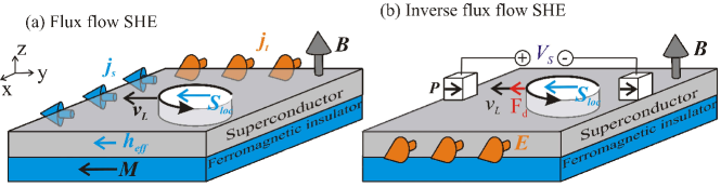
Figure 1: The mechanisms of direct and inverse flux-flow spin Hall effects. The magnetic field $\bm{B}$ perpendicular to film plane creates Abrikosov vortices in superconductor shown by white cylinders surrounded by the circulating current. Vortex cores contain localized normal phase which acquires spin polarization ${\bm{S}}_{loc}$ due to the splitting field induced by ferromagnetic insulator and Zeeman effect. (a) Direct flux-flow SHE. The interaction of transport $\bm{j}_{t}$ and superconducting current circulating around vortex generates the Lorentz force driving vortex lattice motion in the transverse direction with the velocity $\bm{v}_{L}\perp\bm{j}_{t}$. Vortex motion results in the transverse spin current $\bm{j}_{s}$. (b) Inverse flux-flow SHE. The spin-dependent bias $V_{s}$ can be generated by biasing the ferromagnetic electrodes with polarization $\bm{P}$, attached to the superconductor. The induced spin accumulation gradient $\nabla\mu_{z}$ produces the driving force on the vortex lines $\bm{F}_{d}\parallel\nabla\mu_{z}$. In result vortex lattice tend to move in the direction $\bm{v}_{L}\parallel\nabla\mu_{z}$ and produce the average electric field in transverse direction $\bm{E}=\bm{B}\times\bm{v}_{L}/c$.

Below we demonstrate that $\alpha$ becomes the only relevant parameter which determines the amplitude of the pure spin current generated by the vortex motion. The latter can be characterized by the spin Hall angle $\theta_{sH}=ej_{s}/j$, where $j_{s}$ is the induced spin current and and $\bm{j}=\bm{j}_{t}$ is the charge current equal to the transport current generated by the external source. The spin Hall angle can be estimated as $\theta_{sH}\sim\alpha$. At the paramagnetic threshold $h\sim k_{B}T_{c}$ it can reach $\theta_{sH}\sim 1$ which is much larger than the record values $\theta_{sH}<0.1$ obtained in the heavy metal spin current generators [1].

The above result is rather surprising because the maximal spin splitting $h\sim k_{B}T_{c}$ is very small as compared to the Fermi energy $E_{F}$, since in usual superconductors $E_{F}/k_{B}T_{c}\sim 10^{2}-10^{3}$. In this case the polarization, which is the relative difference between spin-up/down conductivities is rather small $\sim h/E_{F}\ll 1$. This limit yields vanishing spin-polarized component of the resistive current. However, it is the vortex motion which generates much larger spin current in the transverse direction $\bm{j}_{s}\perp\bm{j}$ as explained below.

The scheme of the flux-flow direct spin Hall effect is shown in Fig. 1a. Here, we assume that the superconductor with spin-splitting field and vortices is subject to the transport charge current $\bm{j}$ generated by the external source. This transport current induces the Lorenz force acting on the vortex lines in the direction perpendicular to current $\bm{F}_{L}\propto\bm{j}\times\bm{B}$. Provided that the Lorenz force overcomes the pinning barrier, vortices start to move in the transverse direction with the velocity $\bm{v}_{L}\perp\bm{j}$. Taking into account the spin polarization $S_{loc}$ which exists inside each vortex core due to paramagnetic response, this motion generates the transverse pure spin current $\bm{j}_{s}\approx n_{v}\bm{v}_{L}S_{loc}$, where $n_{v}=B/\phi_{0}$ is the vortex density, $\phi_{0}$ is flux quantum.

Vortex cores in diffusive superconductors can be though of as the normal metal tubes, of the diameter determined by the coherence length $\xi$. In the presence of spin splitting field, the vortex cores contain localized spin $S_{loc}\sim\chi_{n}h\xi^{2}$ per unit vortex length, where $\chi_{n}=N_{0}$ is the normal metal paramagnetic susceptibility and $N_{0}$ is the Fermi-level density of states. To estimate $j_{s}$ we substitute the flux-flow vortex velocity $v_{L}=-cE/B$ and get $\theta_{sH}\sim ch/(eDH_{c2})\sim\alpha$, so that $\alpha$ appears to be the only small parameter limiting the spin current generation. The physical reason for large $\theta_{sH}$ lies in the fast motion of vortices which can be compared e.g. with the Drude-model electron drift velocity $\bar{v}=\sigma_{n}E/ne$, where the conductivity is $\sigma_{n}=e^{2}N_{0}D$. At $B\approx H_{c2}$ we have the relation $v_{L}\approx(E_{F}/k_{B}T_{c})\bar{v}\gg\bar{v}$. Therefore spin polarization can be transported much faster by moving vortices than by electrons drifting along the electric field.

Along with the direct SHE we propose also the scheme of the inverse flux-flow SHE shown in Fig. 1b. The mechanism is based on the injection of spin-polarized quasiparticle current into the superconductor by applying the voltage through the spin-filtering ferromagnetic electrodes with polarization $\bm{P}$. The resulting spin-dependent voltage $V_{s}$ generates the spatially-inhomogeneous non-equilibrium spin accumulation which we hereafter denote $\mu_{z}$. Its gradient $\nabla\mu_{z}$ will be shown to produce the longitudinal force acting on the spin-polarized vortex cores pushing them towards one of the ferromagnetic electrodes. The vortex lattice motion with velocity $\bm{v}_{L}$ generates electric field in the transverse direction $\bm{E}\parallel\bm{B}\times\nabla\mu_{s}$ thus providing the novel mechanism of inverse SHE.

Model

To quantify effects discussed above we use the framework of Keldysh-Usadel theory [42, 43] describing the spin current and spin accumulation induced by the vortex motion in the usual $s$-wave spin-singlet superconductor in the diffusive regime[12]. We consider the range of magnetic fields close to $H_{c2}$, neglecting screening and using the Abrikosov solution for the moving vortex lattice. We will show that in addition to the large average spin current there is also the oscillating part which can be considered as the high-frequency source of the spin current at the nearly-terahertz range [44].

We use the formalism of quasiclassical Green’s functions (GF) [42, 43] generalized to describe the non-equilibrium spin states in diffusive superconductors [12], $\check{g}=\left(\begin{array}[]{cc}\hat{g}^{R}&\hat{g}^{K}\\ 0&\hat{g}^{A}\\ \end{array}\right)$, where $\hat{g}^{R/A/K}$ are the retarded/advanced/Keldysh components which are the matrices in spin-Nambu space and depend on two times and a single spatial coordinate variable $\check{g}=\check{g}(t_{1},t_{2},{\bm{r}})$. We consider general expressions for the spin density deviation from the normal state one $S$ and the spin current density $\bm{j}_{s}$ projected on the spin-splitting field direction $\bm{h}$. These quantities are given by the following general expressions

$$S(t,\bm{r})=-(\pi\chi_{n}/8){\rm Tr}[\hat{\tau}_{3}\hat{\sigma}_{h}\hat{g}^{K}(t,t,\bm{r})]$$ (1)

$$\bm{j}_{s}(t,\bm{r})=(\pi\sigma_{n}/8e^{2}){\rm Tr}[\hat{\sigma}_{h}(\hat{g}\circ\hat{\partial}_{\bm{r}}\hat{g})^{K}](t,t,\bm{r}).$$ (2)

Hereafter, $\hat{\sigma}_{h}=(\hat{\sigma}_{1}h_{x}+\hat{\sigma}_{2}h_{y}+\hat{\sigma}_{3}h_{z})/h$ is the operator of the spin projection on the spin-splitting field direction, $\hat{\sigma}_{i}$, $\hat{\tau}_{i}$ with $i=0,1,2,3$ are the Pauli matrices in spin and Nambu spaces, the symbolic time-convolution operator is given by $(A\circ B)(t_{1},t_{2})=\int dtA(t_{1},t)B(t,t_{2})$, the covariant differential superoperator is defined by $\hat{\partial}_{\bm{r}}=\nabla-i\tilde{e}[\hat{\tau}_{3}{\bm{A}},]_{t}$, where $\tilde{e}=e/\hbar c$ and the two-time commutator is defined as $[X,g]_{t}=X(t_{1})g(t_{1},t_{2})-g(t_{1},t_{2})X(t_{2})$, similarly for anticommutator $\{,\}_{t}$.

The general expression for $\bm{j}_{s}$ can be simplified using the following steps. First, due to the normalization condition $(\check{g}\circ\check{g})(t_{1},t_{2})=\check{I}\delta(t_{1}-t_{2})$, where $\check{I}$ is the unit matrix in Keldysh-Nambu-spin space, we introduce the parametrization of Keldysh component in terms of the distribution function $\hat{g}^{K}=\hat{g}^{R}\circ\hat{f}-\hat{f}\circ\hat{g}^{A}$. Second, we introduce mixed representation $\check{g}(t_{1},t_{2})=\int_{-\infty}^{\infty}\check{g}(\varepsilon,t)e^{-i\varepsilon(t_{1}-t_{2})}d\varepsilon/2\pi$, where $t=(t_{1}+t_{2})/2$ and use gradient expansion of the time convolution product in Eq. (2) as explained below.

In the flux-flow regime we assume that vortices move with the constant velocity $\bm{v}_{L}$. In the zero-order approximation the distribution function is equilibrium $\hat{f}(\varepsilon)=f_{0}(\varepsilon)\hat{\tau}_{0}\equiv\tanh[\varepsilon/(2k_{B}T)]\hat{\tau}_{0}$. Similarly, the spectral functions have their equilibrium forms in the frame moving together with vortices $\hat{g}^{R/A}(\bm{r})\approx\hat{g}^{R/A}_{0}(\bm{r}-\bm{v}_{L}t)$. This approximation yields zero spin current which is absent in equilibrium spin-singlet superconductors. Thus, we need to consider corrections in the linear-response regime which is realized provided the vortex velocity $\bm{v}_{L}$ is small enough to neglect Joule heating, pair breaking or vortex-core shrinking effects [45, 46]. For this purpose we take into account first-order terms in the gradient expansion of time convolutions [47, 48] as well as the non-equilibrium corrections to the spectral functions $\hat{g}^{R/A}_{ne}$ and the distribution function $\hat{f}_{ne}=\hat{f}-f_{0}\hat{\tau}_{0}$. In result we get the two parts of spin current $\bm{j}_{s}=\bm{j}_{s1}+\bm{j}_{s2}$ given by

$$\bm{j}_{s1,2}=\frac{\sigma_{n}}{16e^{2}}\int_{-\infty}^{\infty}{\rm Tr}[\hat{\sigma}_{h}\hat{\bm{J}}^{K}_{1,2}]d\varepsilon,$$ (3)

$$\hat{\bm{J}}^{K}_{1}=f_{0}(\hat{\bm{J}}^{R}_{ne}-\hat{\bm{J}}^{A}_{ne}),$$ (4)

$$\hat{\bm{J}}^{R/A}_{ne}=(\hat{g}^{R/A}\hat{\partial}_{r}\hat{g}^{R/A})_{ne}-\frac{i\hbar}{2}(\partial_{t}\hat{g}^{R/A}_{0}\partial_{\varepsilon}\hat{\nabla}\hat{g}^{R/A}_{0}-\partial_{\varepsilon}\hat{g}^{R/A}_{0}\partial_{t}\hat{\nabla}\hat{g}^{R/A}_{0}),$$ (5)

$$\hat{\bm{J}}^{K}_{2}=\hat{\partial}_{r}\hat{f}-\hat{g}^{R}_{0}\hat{\partial}_{r}\hat{f}\hat{g}^{A}_{0}+\hat{\bm{J}}^{R}_{0}\hat{f}_{ne}-\hat{f}_{ne}\hat{\bm{J}}^{A}_{0}.$$ (6)

Although expressions (3,4,5,6) look quite involved, different contributions to the current there have clear physical meanings. The first part of the spin current $\bm{j}_{s1}$ is determined by the non-equilibrium corrections to the spectral quantities while it contains only the equilibrium distribution function. Here $\hat{\bm{J}}_{ne}^{R/A}$ given by Eq.(5) are the deviations of the spectral current densities from equilibrium. In the charge sector these corrections yield the Caroli-Maki part of the flux-flow conductivity [49]. The important difference is that the charge current is determined by the corrections induced by the order parameter distortions in the moving vortex lattice while they do not contribute to the spin current.

The first term in the r.h.s. of (5) incorporates corrections to the spectral GF $g^{R/A}_{ne}$ as well as the electric field term which appears from the expansion of the covariant differential operator[50] $\hat{\partial}_{r}\hat{X}=\hat{\nabla}\hat{X}+e{\bm{E}}\{\hat{\tau}_{3},\partial_{\varepsilon}\hat{X}\}/2$ and $\hat{\nabla}X=\nabla\hat{X}-i\tilde{e}{\bm{A}}[\hat{\tau}_{3},\hat{X}]$. Here we use the gauge with zero electric potential such that electric field is given by $\bm{E}=-\partial_{t}\bm{A}/c$. The second term in the r.h.s. of (5) comes from the linear-order expansion of time convolution. It contains the equilibrium spectral GF in the moving frame $\hat{g}^{R/A}_{0}(\bm{r}-\bm{v}_{L}t)$. The second part of the spin current $\bm{j}_{s2}$ is determined by the non-equilibrium distribution function. This contribution is analogous to the Tompson term in the flux-flow conductivity[51]. Importantly, in the general case the differential operator in the r.h.s. of (6) contains correction from time convolution expansion so that $\hat{\partial}_{r}\hat{f}=\nabla\hat{f}+e\bm{E}\hat{\tau}_{3}\partial_{\varepsilon}f_{0}$. This correction gives contribution to the charge current but drops from the expression for the spin current (3). The nonequilibrium GF is determined by the Keldysh-Usadel equation[42, 43] which should be solved together with the self-consistency equations. In general this problem is very complicated and has never been approached even numerically. However, the regime of high magnetic fields $H_{c2}-B\ll H_{c2}$ allows for significant simplifications based on the existence of the Abrikosov vortex lattice solution for the superconducting order parameter. In this case it is possible to find analytically nonequilibrium corrections to the spectral functions $\hat{g}^{R/A}$ and the components of distribution function $\hat{f}$.

First of all, we employ the analytical expression for the order parameter distribution in the moving vortex lattice. Assuming the particular directions of vortex velocity $\bm{v}_{L}=v_{L}\bm{y}$ and electric field $\bm{E}=E\bm{x}$ we choose the time-dependent vector potential in the form ${\bm{A}}=Bx{\bm{y}}-cEt{\bm{x}}$. Then the order parameter is given by superposition of the first Landau-level nuclei $\mathcal{L}(x)=\exp(-x^{2}/2L_{H}^{2})$, so that $\Delta=b_{0}e^{-2i\tilde{e}Etx}\sum_{n}C_{n}e^{inp(y-v_{L}t)}\mathcal{L}(x-nx_{0})$. Here $b_{0}$ is field dependent amplitude of the gap, $x_{0}=pL_{H}^{2}$ determines the distance between neighbour superconducting nuclei and $L_{H}=1/\sqrt{2\tilde{e}H_{c2}}$ is the magnetic length. For the triangular lattice $C_{n+1}=e^{i(-1)^{n}\pi/4}$, $pL_{H}=\sqrt{\pi\sqrt{3}}$ and for the square one $C_{n}=1$, $pL_{H}=\sqrt{2\pi}$.

Second, we use the known solutions for the equilibrium spectral functions in the vortex lattice near the upper critical field[50]. Here we take into account the spin-splitting field by shifting the quasiparticle energies according to $\varepsilon_{\sigma}=\varepsilon-\sigma h$, where $\sigma=\pm$. Then the spin-up $g^{R/A}_{0+}$ and spin-down $\hat{g}^{R/A}_{0-}$ GFs are given by

$$\hat{g}^{R}_{0\sigma}(\bm{r},\varepsilon)=\left[1+\frac{|\Delta|^{2}}{2(iq+\varepsilon_{\sigma})^{2}}\right]\hat{\tau}_{3}+\frac{i|\Delta|\hat{\tau}_{2}e^{-i\varphi\hat{\tau}_{3}}}{iq+\varepsilon_{\sigma}},$$ (7)

and $\hat{g}_{0}^{A}=-\hat{\tau}_{3}\hat{g}_{0}^{R+}\hat{\tau}_{3}$ for the advanced GF. Here $q=\tilde{e}{\hbar}H_{c2}D$ and the order parameter is $\Delta=|\Delta|e^{i\varphi}$. These spin-polarized spectral functions provide the description of equilibrium spin density modulation in a superconductor with spin-splitting field in the presence of vortex lattices. The periodic spin density patterns calculated for the typical cases of triangular and square lattices are shown in the Fig. 2. The spin polarization demonstrates enhancement at the vortex cores and suppression between vortices where the order parameter is larger. Thus even in the regime of dense vortex lattices there is an excess spin polarization $S_{loc}$ localized in the vortex cores. It is natural to expect that the motion of such spin-polarized vortices will produce pure spin currents.

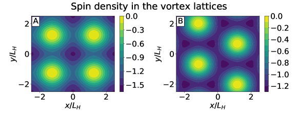
Figure 2: Spin density modulation in the vortex cores . Normalized deviation of the total spin density from the normal metal background, $S/S_{n}$, on square (A) and triangular (B) lattices. Here $S_{n}=-\chi_{n}h$ is spin polarization of the normal metal and $S/S_{n}$ is shown in the units of dimensionless order parameter amplitude $\langle\Delta^{2}\rangle/(k_{B}T_{c})^{2}$. Calculations were performed at low-temperatures, $T\ll T_{c}$, for effective Maki parameter $\alpha=0.5$.

Below we demonstrate the presence of these spin currents by an explicit calculation in the flux-flow regime considering the non-equilibrium situation when the vortex lattice moves under the action of the transport current $\bm{j}_{t}$. We will calculate the spin current density induced by the vortex motion as well as the non-equilibrium spin accumulation and charge imbalance near the vortex cores.

Results

Spin current

To find the contribution $\bm{j}_{s1}$ to spin current density using Eq.(4) we need the non-equilibrium corrections for the spectral functions. In the linear response approximation, assuming that the non-equilibrium corrections are small we can find them using the normalization conditions for quasiclassical propagators $(\hat{g}^{R}\circ\hat{g}^{R})(t_{1},t_{2})=\hat{I}\delta(t_{1}-t_{2})$. The calculation detailed in the Supplementary Information yields the expression for the first term in Eq. (5) through the derivatives of the equilibrium GFs $(\hat{g}^{R}\hat{\nabla}\hat{g}^{R})_{ne}=i\hbar\hat{\nabla}(\partial_{t}\hat{g}^{R}_{0}\partial_{\varepsilon}\hat{g}^{R}_{0}-\partial_{\varepsilon}\hat{g}^{R}_{0}\partial_{t}\hat{g}^{R}_{0})/4$. Hence the spectral spin current density is given by $\hat{\bm{J}}^{R}=i\hbar(\partial_{\varepsilon}\hat{g}_{0}^{R}\hat{\nabla}\partial_{t}\hat{g}_{0}^{R}-\partial_{t}\hat{g}_{0}^{R}\hat{\nabla}\partial_{\varepsilon}\hat{g}_{0}^{R})/2$. In the linear response approximation we keep only the first-order time derivatives $\partial_{t}\hat{g}^{R/A}_{0}=-(\bm{v}_{L}\nabla)\hat{g}^{R/A}_{0}$. In the considered high-field regime $H_{c2}-B\ll H_{c2}$ the order parameter is described by the Abrikosov vortex lattice solution. Thus we can use spectral functions $\hat{g}^{R/A}_{0}=\hat{g}^{R/A}_{0}(\bm{r}-\bm{v}_{L}t,\varepsilon)$ given by the Eq.(7). Substituting the above spectral current density into the Eq.(3) and transforming the energy integral to the summation over Matsubara frequencies we obtain the first part of the spin current

$$\bm{j}_{s1}=-\frac{\hbar\sigma_{n}}{16e^{2}}\frac{{\rm Im}\Psi^{(2)}}{(\pi k_{B}T)^{2}}{\rm Re}[\Delta(\hat{\Pi}\partial_{t}\Delta)^{\ast}-\partial_{t}\Delta(\hat{\Pi}\Delta)^{\ast}],$$ (8)

where $\Psi=\Psi[1/2+(q+ih)/(2\pi k_{B}T)]$ is digamma function, $\Psi^{(n)}(z)=d^{n}\Psi(z)/dz^{n}$ and $\hat{\Pi}=\nabla-2i\tilde{e}\bm{A}$. This part of the spin current has the non-zero space- and time-average $\langle\bm{j}_{s}\rangle=\langle\bm{j}_{s1}\rangle$ determined by the following expression which derivation is shown in the Supplementary Information,

$$\langle\bm{j}_{s}\rangle=-\bm{v}_{L}\sigma_{n}\frac{\hbar\langle\Delta^{2}\rangle{\rm Im}\Psi^{(2)}}{(4\pi k_{B}TeL_{H})^{2}},$$ (9)

where $\langle\Delta^{2}\rangle=\sqrt{\pi}|b_{0}|^{2}L_{H}/x_{0}$ is the order parameter average over the vortex lattice cell. At the same time the average spin density deviation from the normal state induced by the superconducting correlations reads as $\langle S\rangle=-\chi_{n}\langle\Delta^{2}\rangle{\rm Im}\Psi^{(1)}/(4\pi T)$. Therefore, at low temperatures $T\to 0$ we obtain the asymptotic relation $\langle\bm{j}_{s}\rangle=-2\bm{v}_{L}\langle S\rangle/(1+\alpha^{2})$.

The spin current magnitude depends on the order parameter amplitude $b_{0}$ which is determined by the magnetic field. In the limit of large Ginzburg-Landau parameter we get the usual expression for the average gap function[52, 53] $\langle\Delta^{2}\rangle=-8\pi k_{B}Tq\delta B{\rm Re}\Psi^{(1)}/(\beta_{L}H_{c2}{\rm Re}\Psi^{(2)})$, where $\delta B=H_{c2}-B$ is the deviation of external field from the upper critical one, the Abrikosov parameter equals $\beta_{L}=1.16$ for the triangular and $\beta_{L}=1.18$ for the square lattice[54]. In the limit of low temperatures it can be simplified to $\langle\Delta^{2}\rangle=(1-B/H_{c2})(4q^{2}/\beta_{L})(1+\alpha^{2})/(1-\alpha^{2})$ yielding the following analytical expression for the spin Hall angle, $\theta_{sH}=e\langle\bm{j}_{s}\rangle/\bm{j}_{t}$, as a function of the average magnetic induction at low temperatures,

$$\theta_{sH}(B)=-\frac{4\alpha}{\beta_{L}(1-\alpha^{4})}\left(1-\frac{B}{H_{c2}}\right).$$ (10)

The growth of $\theta_{sH}(B)$ with decreasing $B$ given by Eq.(10) close to $H_{c2}$ should continue at lower fields until the order parameter between vortices becomes fully developed at $B\approx 0.3H_{c2}$. In this regime we expect $\theta_{sH}\propto\alpha$ without any small parameters so that $\theta_{sH}\sim 1$ for large exchange splitting $h\sim k_{B}T_{c}$. At smaller fields $B\ll H_{c2}$ the spin Hall angle should decrease as $\theta_{sH}\propto B/H_{c2}$, being proportional to the concentration of vortices. Besides that, according to Eq. (10) large spin Hall angle can be obtained already in the regime $(1-B/H_{c2})\ll 1$ provided that $1-\alpha\ll 1-B/H_{c2}$. Note that we restrict our consideration to $\alpha<1$ when the superconducting transition at $B=H_{c2}$ is of the second order [55, 20].

Now let us consider the second contribution to the spin current $\bm{j}_{s2}$ which according to the Eq.(6) is determined by the non-equilibrium components of the distribution function generated by the vortex lattice motion. Due to the smallness of the order parameter in the regime $H_{c2}-B\ll H_{c2}$ this spin current contribution can be written in terms of the non-equilibrium spin accumulation $\bm{j}_{s2}=(\sigma_{n}/e^{2})\nabla\mu_{s1}$. Here $\mu_{s1}=\int_{-\infty}^{\infty}f_{T3}(\varepsilon)d\varepsilon/2$ is the contribution to the spin accumulation determined by spin-dependent component of the distribution function $f_{T3}={\rm Tr}[\hat{\sigma}_{h}\hat{f}]/4$, which can be considered as the spin-dependent shift of the chemical potential [5]. Since $\mu_{s1}$ has to be periodic function, its gradients cannot provide non-zero space-average or time-average spin current, however this contribution is also of interest since it produces AC component of $\bm{j}_{s}$. To find it, we need to solve the kinetic equation for the spin imbalance, which is similar to that for the longitudinal distribution function [50]

$$\nabla^{2}f_{T3}=-e\bm{E}\bm{J}_{se}\partial_{\varepsilon}f_{0}-\frac{1}{8D}\partial_{\varepsilon}f_{0}{\rm Tr}[\hat{\sigma}_{h}\partial_{t}\hat{\Delta}(\hat{g}^{R}_{0}-\hat{g}^{A}_{0})].$$ (11)

Here $\bm{J}_{se}={\rm Tr}[\hat{\tau}_{3}\hat{\sigma}_{h}(\hat{\bm{J}}^{R}_{0}-\hat{\bm{J}}^{A}_{0})]/8$ is spectral spin-energy current density [11] and the gap operator in the second term of the r.h.s. is $\hat{\Delta}=i|\Delta|\hat{\tau}_{2}e^{-i\varphi\hat{\tau}_{3}}$. For the general-form Abrikosov vortex lattice, Eq.(11) can be solved analytically yielding

$$\mu_{s1}=\tilde{e}\hbar v_{L}H_{c2}F_{0}\sum_{n}\sin(py+\phi_{n})F(x-nx_{0})$$ (12)

$$F(x)=\int_{-\infty}^{\infty}e^{-p|x-x^{\prime}|}\mathcal{L}(x^{\prime}-x_{0})\mathcal{L}(x^{\prime})dx^{\prime},$$ (13)

$$F_{0}=\langle\Delta^{2}\rangle\frac{pL_{H}}{2\sqrt{\pi}}\left(\frac{{\rm Im}\Psi^{(2)}}{(2\pi k_{B}T)^{2}}-\frac{{\rm Im}\Psi^{(1)}}{2\pi qk_{B}T}\right)$$ (14)

and $\phi_{n}={\rm arg}(C_{n}^{\ast}C_{n+1})$, see Supplementary Information.

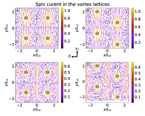
Figure 3: Spin current density generated by the vortex lattice motion. (A,B) The total spin current $\bm{j}_{s}$ for square and triangular spin lattices generated by the vortex lattice motion, normalized by $v_{L}\chi_{n}\langle\Delta^{2}\rangle/(k_{B}T_{c})$. (C,D) Deviation of the net spin current from its spatial average $\tilde{\bm{j}}_{s}=\bm{j}_{s}-\langle\bm{j}_{s}\rangle$. Gray circles correspond to the position of the vortexes. Left/right columns describe the case of the square/triangular lattices, respectively. Arrows between panels indicate the direction of the vortex velocity $\bm{v}_{L}$ and average electric field $\bm{E}$. Calculations were performed at low-temperatures, $T\ll T_{c}$, for $\alpha=0.5$.

The overall distributions spin currents are shown in Fig. 3 produced using the Matplotlib package[56] for two different vortex lattice geometries. Here one can see that the spin current mostly flows along the vortex chains with maximal current concentrated in the vortex cores. This result confirms our initial qualitative picture shown in Fig. 1 that the spin is transported by the moving spin-polarized vortex cores. In addition, in Figs. 3C,D one can see a non-trivial distribution of the spatially-periodic part of the current $\tilde{\bm{j}}_{s}=\bm{j}_{s}-\langle\bm{j}_{s}\rangle$, which is important for the AC spin current generation discussed below. The periodic part $\tilde{\bm{j}}_{s}$ forms two standing eddies localized close to the vortex core similar to that which are formed by the low-Reynolds viscous flow past a cylinder.

Spin accumulation and charge imbalance

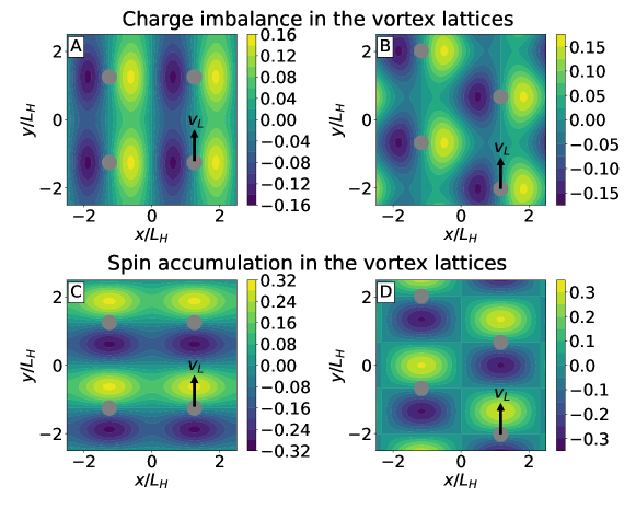
Figure 4: Charge imbalance $\mu$ (A,B) and spin accumulation $\mu_{z}$ (C,D) generated by the moving vortex lattices. Both quantities are normalized to $\hbar v_{L}\langle\Delta^{2}\rangle/(L_{H}q^{2})$. Left/right columns describe the case of the square/triangular lattices, respectively. Gray circles correspond to the position of the vortex cores and black arrows indicate the direction of the vortex velocity $\bm{v}_{L}$. Calculations were performed at low-temperatures, $T\ll T_{c}$, for $\alpha=0.5$.

Besides generating the spin current, moving vortices produce other types of non-equilibrium states in the superconductor, such as the charge imbalance and the non-equilibrium spin accumulation which we denote as $\mu$ and $\mu_{z}$, respectively. These quantities has been widely used as the experimentally observable characteristics of the non-equilibrium superconducting states both in spin -degenerate[57, 58, 59, 60, 61, 62, 63, 64] and spin-split systems [15, 65, 16, 13, 24, 26, 14]. General expressions for charge imbalance and spin accumulation in terms of the quasiclassical GF read as

$$\mu=-(\pi/8){\rm Tr}\hat{g}^{K}_{ne}(t,t,\bm{r})$$ (15)

$$\mu_{s}=-(\pi/8){\rm Tr}[\hat{\tau}_{3}\hat{\sigma}_{h}\hat{g}^{K}_{ne}](t,t,\bm{r})$$ (16)

where $\hat{g}^{K}_{ne}$ is non-equilibrium part of Keldysh GF. To find $\mu$ and $\mu_{s}$ using the expressions (15,16) we employ the mixed representation with the first-order gradient expansion of the non-equilibrium part of Keldysh GF, $\hat{g}^{K}_{ne}=(\hat{g}^{R}\hat{f}-\hat{f}\hat{g}^{A})_{ne}-i\hbar\partial_{\varepsilon}f_{0}\partial_{t}(\hat{g}^{R}_{0}+\hat{g}^{A}_{0})/2$. The spin accumulation $\mu_{z}$ is determined by spin imbalance mode $f_{T3}$ and time derivative of spectral GF so that close to $H_{c2}$ we have

$$\mu_{s}=-\mu_{s1}+\frac{\hbar v_{L}}{4}\frac{{\rm Im}\Psi^{(2)}}{(2\pi T)^{2}}\partial_{y}|\Delta|^{2}.$$ (17)

To obtain the second term in (17) we integrated $\partial_{\varepsilon}f_{0}{\rm Tr}[\hat{\tau}_{3}\hat{\sigma}_{3}\partial_{t}(\hat{g}^{R}_{0}+\hat{g}^{A}_{0})]$ over energy by parts and transformed result to the sum over Matsubara frequencies. The details of this calculation can be checked in the Supplementary Information.

To calculate charge imbalance generated by moving vortex lattice we notice that term with time derivatives of spectral GF in $\hat{g}^{K}_{ne}$ is traced out, while non-equilibrium corrections to spectral functions are of importance. The latter can be found with the help of normalization condition which results in the leading order in $|\Delta|$ in ${\rm Tr}\hat{g}^{R/A}_{ne}=\pm\frac{i\hbar}{4}{\rm Tr}([\hat{\tau}_{3},\partial_{t}\hat{g}_{0}^{R/A}]\partial_{\varepsilon}\hat{g}_{0}^{R/A})$. Therefore

$$\mu=-\mu_{1}-\frac{\hbar v_{L}}{8}\frac{{\rm Re}\Psi^{(2)}}{(2\pi T)^{2}}\partial_{x}|\Delta|^{2},$$ (18)

where $\mu_{1}=\int_{-\infty}^{\infty}f_{T}d\varepsilon/2$ is contribution to the electrostatic potential from transverse component of distribution function, $f_{T}={\rm Tr}[\hat{\tau}_{3}\hat{f}]/4$. For high magnetic fields kinetic equation for $f_{T}$ reads as

$$\nabla^{2}f_{T}=-e\partial_{\varepsilon}f_{0}\nabla({\cal D}_{T}{\bm{E}})+\frac{1}{8D}\partial_{\varepsilon}f_{0}{\rm Tr}[\hat{\tau}_{3}\partial_{t}\hat{\Delta}(\hat{g}^{R}+\hat{g}^{A})],$$ (19)

where ${\cal D}_{T}={\rm Tr}(\hat{\tau}_{0}\hat{\sigma}_{0}-\hat{\tau}_{3}\hat{g}^{R}\hat{\tau}_{3}\hat{g}^{A})/8$. By using Abrikosov vortex-lattice solution, spatially periodic solution of kinetic equation can be found analytically, the reader can consult Supplementary Information for the details of this derivation.

Distributions of $\mu$ and $\mu_{z}$ generated by the moving square and triangular vortex lattices are shown in Fig. 4. The patterns of charge imbalance agree with the qualitative picture suggested by Bardeen and Stephen [66] where the vortex motion is accompanied by the generation of dipolar-like electric field near the vortex core, corresponding to the electric dipole directed perpendicular to the vortex velocity $\bm{v}_{L}$. On the contrary, the "spin dipoles" corresponding to the patterns of $\mu_{z}$ are directed along $\bm{v}_{L}$. Note also, that spin accumulation is proportional to the generalized Maki parameter, while $\mu$ remains finite when $\alpha\to 0$, that is paramagnetic effects are neglected.

Inverse flux-flow spin Hall effect

We suggest the new mechanism of the inverse flux-flow SHE which is based on the previously unknown effect of longitudinal vortex motion driven by the spin current or spin accumulation injected into the superconductor from the attached ferromagnetic electrodes with polarization $\bm{P}$. We denote $V_{s}$ the corresponding spin-dependent external bias. For simplicity we assume that the polarization is aligned with the spin-splitting filed in the superconductor $\bm{P}\parallel\bm{h}$. To calculate the force acting on vortex from the injected spin current we consider the regime of temperatures close to the critical one $T_{c}$. In this case we can neglect the superconducting corrections to the density of states. This assumption simplifies expression for spin-dependent part of the distribution function which can be taken in the form corresponding to the normal metal $f_{T3}(\bm{r})=\mu_{z}(\bm{r})\partial_{\varepsilon}f_{0}$ where $\mu_{z}=\mu_{z}(\bm{r})$ is the spatially-inhomogeneous spin accumulation generated by the external bias $V_{s}$. Besides that here we consider the regime of small fields $B\ll H_{c2}$ when vortices can be considered as individual objects. The force acting on the single vortex from non-equilibrium spin-polarized environment $\bm{F}_{d}$ can be calculated using the known general expression [47, 48]. Near the critical temperature when $|\Delta|\ll k_{B}T$ we obtain the simple analytical result $\bm{F}_{d}\approx-\nabla\mu_{z}S_{loc}|\Delta|^{2}/(k_{B}T_{c})^{2}$, where $S_{loc}$ is the total spin localized in the vortex core. This driving force, balanced by the friction $\bm{F}_{v}=-\rho\bm{v}_{L}$, where $\rho$ is the vortex viscosity coefficient, yields the flux-flow velocity $\bm{v}_{L}\parallel\nabla\mu_{z}$. Its absolute value can be found using the known analytical expression for viscosity coefficient $\rho=\phi_{0}\sigma_{n}\beta H_{c2}/c^{2}$. The temperature dependence close to $T_{c}$ is determined by the coefficient $\beta=\beta_{0}/\sqrt{1-T/T_{c}}$, where $\beta_{0}$ is some numerical value[67, 68, 69]. Taking into account that the concentration of vortices is determined by the average magnetic induction $B$ and using the usual expression for the sample-average electric field $\bm{E}=-\bm{v}_{L}\times\bm{B}/c$ we obtain the relation

$$\frac{eE}{\nabla\mu_{s}}\approx\frac{h}{q}\frac{|\Delta|^{2}}{(k_{B}T_{c})^{2}}\frac{B}{H_{c2}}\sqrt{1-\frac{T}{T_{c}}}.$$ (20)

The obtained result (20) yields the linear response relation for the inverse spin Hall effect because the electric field $E$ and the corresponding electric current are generated in response to the applied spin-dependent voltage $V_{s}$. The overall temperature dependence of the generated electric field $E\propto(1-T/T_{c})^{3/2}$ is determined by the order parameter amplitude $\Delta^{2}\propto(1-T/T_{c})$ and the additional factor which comes from the divergence of vortex viscosity coefficient close to the critical temperature[70] $\rho\propto 1/\sqrt{1-T/T_{c}}$.

Discussion and conclusions

We have found the spin current generation by moving vortices which penetrate the whole volume of the type-II superconductor. Thus the obtained spin current in contrast to the previously known schemes based on the injection mechanisms exists everywhere in the sample volume and is prone to the spin relaxation mechanisms such as the spin-flip scattering. The predicted spin current generation can be tested in the open circuit geometries when the vortices annihilate at the insulating boundary. In this case the net spin current at the boundary, $y=0$, should vanish $j_{sy}(y=0)=0$ generating the surface spin accumulation $V_{s}=\mu_{z}(y=0)/e$ which can be measured by the ferromagnetic detector electrodes [13, 14, 15, 16]. In the regime when spin relaxation length $l_{s}$ is much larger than the intervortex distance, the time-average spin accumulation at low temperatures reads as $V_{s}=-l_{s}\theta_{sH}Ee^{-y/l_{s}}$.

The second possible experimental test is based on the direct measurement of the spin current injected through superconductor interfaces into the inverse spin Hall detector[71, 72]. This approach allows to measure both the DC and the high-frequency AC spin current signals. The latter is generated due to the periodic structure of moving vortex lattice. The distribution of the space-periodic spin current component is shown in Fig.3C,D. The amplitude of AC component flowing through the superconductor interface, $\langle\tilde{j}_{sy}\rangle_{x}$, is determined by the variations of the current average along the boundary, $\langle j_{sy}\rangle_{x}$, with respect to the constant background current $\langle j_{s}\rangle$. At low temperatures, the relative magnitude is given by $\langle\tilde{j}_{sy}\rangle_{x}/\langle j_{s}\rangle=(1-\langle\Delta^{2}\rangle_{x}/\langle\Delta^{2}\rangle)(1+\alpha^{2})/2$. According to the recent measurements, the frequency of vortex entry into the superconducting sample can reach dozens of gigahertz in Pb [44] and the teraherz range in layered high-temperature superconductors [73]. In the suggested setup this is the frequency of the AC spin current generated by the vortex motion. The suggested high-frequency spin current generation can be useful in antiferromagnetic spintronics characterized by the terahertz-range dynamics of the magnetic system[74].

Traditionally the charge imbalance and spin accumulation has been accessed experimentally using non-local conductance measurements [61, 63, 64, 58, 15, 65, 16, 13, 24, 26, 14], when the non-equilibrium states were created by the current in the injector circuit. The non-local electric signal has been measured between the normal detector electrodes, either ferromagnetic or non-ferromagnetic attached to the different points of superconducting sample. Here we show that in the flux-flow regime the non-equilibrium states with non-zero charge imbalance $\mu$ and spin accumulation $\mu_{z}$ appear in the absence of quasiparticle injector current, but rather just due to the vortex motion. The quantities $\mu$ and $\mu_{z}$ can be measured using the same electrical detection circuits as in the non-local conductance measurement setups. For example, the tunneling current at the non-ferromagnetic normal detector electrode is proportional to $\mu$. In case of the ferromagnetic electrode there is a contribution to the detector current[5] proportional to $\mu_{z}$. In the flux-flow regime each vortex carries the distributions of $\mu$ and $\mu_{z}$ localized in the vortex core. Thus, moving vortices passing close to the detector electrode are expected to generate pulses of the tunneling current or voltage, depending on the detection scheme. This provides a tool capable for detecting the motion of individual vortices. In contrast to the magnetometer techniques it does not have the frequency limitations[44] and therefore can directly resolve the ultrafast vortex motion with the frequencies up to the dozens of gigahertz .

To conclude, we have demonstrated fundamental mechanisms of direct and inverse spin Hall effects due to the flux-flow of Abrikosov vortices in type-II superconductors. The pure spin current carried by the fast vortices moving in the transverse direction is characterized by the large spin Hall angle which in general does not contain any small parameters. Besides that there is also an AC component which appears due to the periodic structure of the vortex lattice. The AC spin current has the same order of magnitude as the average one. This effect can be used for the generation of spin signals in wide frequency domain up to the range of therahertz. We pointed out the longitudinal driving force exerted on vortex by the injected spin current. The vortex motion generated by this force leads to the inverse spin Hall effect. This mechanism can be applied for flux-flow based detection of pure spin currents.

Author contributions

Both authors, AV and MS contributed equally to calculations and writing of the manuscript.

Additional information

Supplementary information accompanies this paper.

Competing Interests: The authors declare that they have no competing interests.

Data availability: No datasets were generated or analysed during the current study.

References

- [1] Sinova, J., Valenzuela, S. O., Wunderlich, J., Back, C. H. & Jungwirth, T. Spin hall effects. \JournalTitleRev. Mod. Phys. 87, 1213–1260 (2015).
- [2] Abanin, D. A. et al. Giant nonlocality near the dirac point in graphene. \JournalTitleScience 332, 328 (2011).
- [3] Abanin, D. A., Gorbachev, R. V., Novoselov, K. S., Geim, A. K. & Levitov, L. S. Giant spin-hall effect induced by the zeeman interaction in graphene. \JournalTitlePhys. Rev. Lett. 107, 096601 (2011).
- [4] Wei, P. et al. Strong interfacial exchange field in the graphene/eus heterostructure. \JournalTitleNature Materials 15, 711 (2016).
- [5] Bergeret, F., Silaev, M., Virtanen, P. & Heikkila, T. Nonequilibrium effects in superconductors with a spin-splitting field. \JournalTitlearXiv:1706.08245 (2017). Accepted to Rev. Mod. Phys.
- [6] Tedrow, P. M. & Meservey, R. Spin-dependent tunneling into ferromagnetic nickel. \JournalTitlePhys. Rev. Lett. 26, 192–195 (1971).
- [7] Silaev, M., Virtanen, P., Bergeret, F. S. & Heikkilä, T. T. Long-range spin accumulation from heat injection in mesoscopic superconductors with zeeman splitting. \JournalTitlePhys. Rev. Lett. 114, 167002 (2015).
- [8] Bobkova, I. V. & Bobkov, A. M. Long-range spin imbalance in mesoscopic superconductors under zeeman splitting. \JournalTitleJETP Letters 101, 118–124 (2015).
- [9] Krishtop, T., Houzet, M. & Meyer, J. S. Nonequilibrium spin transport in zeeman-split superconductors. \JournalTitlePhys. Rev. B 91, 121407 (2015).
- [10] Virtanen, P., Heikkilä, T. T. & Bergeret, F. S. Stimulated quasiparticles in spin-split superconductors. \JournalTitlePhys. Rev. B 93, 014512 (2016).
- [11] Aikebaier, F., Silaev, M. A. & Heikkilä, T. T. Supercurrent-induced charge-spin conversion in spin-split superconductors. \JournalTitlePhys. Rev. B 98, 024516, DOI: 10.1103/PhysRevB.98.024516 (2018).
- [12] Bergeret, F. S., Silaev, M., Virtanen, P. & Heikkilä, T. T. Nonequilibrium effects in superconductors with a spin-splitting field (2017). arXiv:1706.08245.
- [13] Hübler, F., Wolf, M. J., Beckmann, D. & v. Löhneysen, H. Long-range spin-polarized quasiparticle transport in mesoscopic al superconductors with a zeeman splitting. \JournalTitlePhys. Rev. Lett. 109, 207001 (2012).
- [14] Wolf, M. J., Sürgers, C., Fischer, G. & Beckmann, D. Spin-polarized quasiparticle transport in exchange-split superconducting aluminum on europium sulfide. \JournalTitlePhys. Rev. B 90, 144509 (2014).
- [15] Quay, C. H. L., Chevallier, D., Bena, C. & Aprili, M. Spin imbalance and spin-charge separation in a mesoscopic superconductor. \JournalTitleNat Phys 9, 84–88 (2013).
- [16] Quay, C. H. L., Dutreix, C., Chevallier, D., Bena, C. & Aprili, M. Frequency-domain measurement of the spin-imbalance lifetime in superconductors. \JournalTitlePhys. Rev. B 93, 220501 (2016).
- [17] Maki, K. Effect of pauli paramagnetism on magnetic properties of high-field superconductors. \JournalTitlePhys. Rev. 148, 362–369 (1966).
- [18] Chandrasekhar, B. S. A note on the maximum critical field of high-field superconductors. \JournalTitleAppl. Phys. Lett. 1, 7–8, DOI: 10.1063/1.1777362 (1962).
- [19] Clogston, A. M. Upper limit for the critical field in hard superconductors. \JournalTitlePhys. Rev. Lett. 9, 266–267 (1962).
- [20] Saint-James, D., Sarma, G. & Thomas, E. Type II Superconductivity. Commonwealth and International Library. Liberal Studies Divi (Elsevier Science & Technology, 1969).
- [21] Gurevich, A. Upper critical field and the fulde-ferrel-larkin-ovchinnikov transition in multiband superconductors. \JournalTitlePhys. Rev. B 82, 184504 (2010).
- [22] Cho, K. et al. Anisotropic upper critical field and possible fulde-ferrel-larkin-ovchinnikov state in the stoichiometric pnictide superconductor lifeas. \JournalTitlePhys. Rev. B 83, 060502 (2011).
- [23] Tedrow, P. M., Meservey, R. & Schwartz, B. B. Experimental evidence for a first-order magnetic transition in thin superconducting aluminum films. \JournalTitlePhys. Rev. Lett. 24, 1004–1007, DOI: 10.1103/PhysRevLett.24.1004 (1970).
- [24] Kolenda, S., Wolf, M. J. & Beckmann, D. Observation of thermoelectric currents in high-field superconductor-ferromagnet tunnel junctions. \JournalTitlePhys. Rev. Lett. 116, 097001 (2016).
- [25] Fulde, P. & Ferrell, R. A. Superconductivity in a strong spin-exchange field. \JournalTitlePhys. Rev. 135, A550–A563, DOI: 10.1103/PhysRev.135.A550 (1964).
- [26] Kolenda, S., Sürgers, C., Fischer, G. & Beckmann, D. Thermoelectric effects in superconductor-ferromagnet tunnel junctions on europium sulfide. \JournalTitlePhys. Rev. B 95, 224505 (2017).
- [27] Strambini, E. et al. Revealing the magnetic proximity effect in eus/al bilayers through superconducting tunneling spectroscopy. \JournalTitlePhys. Rev. Materials 1, 054402 (2017).
- [28] Yao, Y. et al. Probe of spin dynamics in superconducting nbn thin films via spin pumping. \JournalTitlePhys. Rev. B 97, 224414, DOI: 10.1103/PhysRevB.97.224414 (2018).
- [29] Tokuyasu, T., Sauls, J. A. & Rainer, D. Proximity effect of a ferromagnetic insulator in contact with a superconductor. \JournalTitlePhys. Rev. B 38, 8823–8833, DOI: 10.1103/PhysRevB.38.8823 (1988).
- [30] Heikkilä, T. T., Ojajärvi, R., Maasilta, I. J., Giazotto, F. & Bergeret, F. Thermoelectric radiation detector based on superconductor/ferromagnet systems (2017). arXiv:1709.08856.
- [31] Virtanen, P., Bergeret, F. S., Strambini, E., Giazotto, F. & Braggio, A. Majorana bound states in hybrid two-dimensional josephson junctions with ferromagnetic insulators. \JournalTitlePhys. Rev. B 98, 020501, DOI: 10.1103/PhysRevB.98.020501 (2018).
- [32] Chandrasekhar, B. S. A note on the maximum critical field of high-field superconductors. \JournalTitleAppl. Phys. Lett. 1, 7–8, DOI: 10.1063/1.1777362 (1962).
- [33] Clogston, A. M. Upper limit for the critical field in hard superconductors. \JournalTitlePhys. Rev. Lett. 9, 266–267, DOI: 10.1103/PhysRevLett.9.266 (1962).
- [34] Larkin, A. I. & Ovchinnikov, Y. N. Inhomogeneous state of superconductors. \JournalTitleSov. Phys. JETP 20, 762–769 (1965).
- [35] Aslamazov, L. Influence of impurities on the existence of an inhomogeneous state in a ferromagnetic superconductor. \JournalTitleJournal of Experimental and Theoretical Physics 28, 773 (1969).
- [36] Buzdin, A. I. Proximity effects in superconductor-ferromagnet heterostructures. \JournalTitleRev. Mod. Phys. 77, 935–976 (2005).
- [37] Yao, Y. et al. Probe of spin dynamics in superconducting nbn thin films via spin pumping (2017). arXiv:1710.10833.
- [38] Buzdin, A. I., Bulaevskiĭ, L. N., Kulich, M. L. & Panyukov, S. V. Magnetic superconductors. \JournalTitleSoviet Physics Uspekhi 27, 927 (1984).
- [39] Müller, K.-H. & Narozhnyi, V. N. Interaction of superconductivity and magnetism in borocarbide superconductors. \JournalTitleReports on Progress in Physics 64, 943 (2001).
- [40] Bluhm, H., Sebastian, S. E., Guikema, J. W., Fisher, I. R. & Moler, K. A. Scanning hall probe imaging of . \JournalTitlePhys. Rev. B 73, 014514 (2006).
- [41] DeBeer-Schmitt, L. et al. Pauli paramagnetic effects on vortices in superconducting . \JournalTitlePhys. Rev. Lett. 99, 167001 (2007).
- [42] Schmid, A. & Schön, G. Linearized kinetic equations and relaxation processes of a superconductor near t c. \JournalTitleJournal of Low Temperature Physics 20, 207–227 (1975).
- [43] Belzig, W., Wilhelm, F. K., Bruder, C., Schön, G. & Zaikin, A. D. Quasiclassical green’s function approach to mesoscopic superconductivity. \JournalTitleSuperlattices and Microstructures 25, 1251–1288 (1999).
- [44] Embon, L. et al. Imaging of super-fast dynamics and flow instabilities of superconducting vortices. \JournalTitleNature Communications 8, 85 (2017).
- [45] Larkin, A. I. & Ovchinnikov, Y. N. \JournalTitleSov. Phys. JETP 41, 960 (1976).
- [46] Klein, W., Huebener, R. P., Gauss, S. & Parisi, J. \JournalTitleJ. Low Temp. Phys. 61, 413 (1985).
- [47] Larkin, A. I. & Ovchinnikov, Y. N. In Langenberg, D. N. & Larkin, A. (eds.) Modern Problems in Condensed Matter Sciences: Nonequilibrium Superconductivity, 493 (Elsevier, 1986).
- [48] Kopnin, N. B. Theory of Nonequilibrium Superconductivity (Oxford University Press, 2001).
- [49] Caroli, C. & Maki, K. Motion of the vortex structure in type-ii superconductors in high magnetic field. \JournalTitlePhys. Rev. 164, 591–607, DOI: 10.1103/PhysRev.164.591 (1967).
- [50] Silaev, M. & Vargunin, A. Vortex motion and flux-flow resistivity in dirty multiband superconductors. \JournalTitlePhys. Rev. B 94, 224506 (2016).
- [51] Thompson, R. S. Microwave, flux flow, and fluctuation resistance of dirty type-ii superconductors. \JournalTitlePhys. Rev. B 1, 327–333, DOI: 10.1103/PhysRevB.1.327 (1970).
- [52] Caroli, C., Cyrot, M. & de Gennes, P. G. The magnetic behavior of dirty superconductors. \JournalTitleSolid State Communications 4, 17–19 (1966).
- [53] Silaev, M. Magnetic behavior of dirty multiband superconductors near the upper critical field. \JournalTitlePhys. Rev. B 93, 214509 (2016).
- [54] Kleiner, W. H., Roth, L. M. & Autler, S. H. Bulk solution of ginzburg-landau equations for type ii superconductors: Upper critical field region. \JournalTitlePhys. Rev. 133, A1226–A1227 (1964).
- [55] Maki, K. \JournalTitleJ. Low Temp. Phys. 1, 45 (1969).
- [56] Hunter, J. D. Matplotlib: A 2d graphics environment. \JournalTitleComputing In Science & Engineering 9, IEEE COMPUTER SOC—95 (2007).
- [57] Yagi, R. Charge imbalance observed in voltage-biased superconductor–normal tunnel junctions. \JournalTitlePhys. Rev. B 73, 134507, DOI: 10.1103/PhysRevB.73.134507 (2006).
- [58] Hübler, F., Lemyre, J. C., Beckmann, D. & v. Löhneysen, H. Charge imbalance in superconductors in the low-temperature limit. \JournalTitlePhys. Rev. B 81, 184524, DOI: 10.1103/PhysRevB.81.184524 (2010).
- [59] Tinkham, M. & Clarke, J. Theory of pair-quasiparticle potential difference in nonequilibrium superconductors. \JournalTitlePhys. Rev. Lett. 28, 1366–1369 (1972).
- [60] Tinkham, M. Tunneling generation, relaxation, and tunneling detection of hole-electron imbalance in superconductors. \JournalTitlePhys. Rev. B 6, 1747–1756 (1972).
- [61] Clarke, J., Fjordbøge, B. R. & Lindelof, P. E. Supercurrent-induced charge imbalance measured in a superconductor in the presence of a thermal gradient. \JournalTitlePhys. Rev. Lett. 43, 642–645, DOI: 10.1103/PhysRevLett.43.642 (1979).
- [62] Clarke, J. & Tinkham, M. Theory of quasiparticle charge imbalance induced in a superconductor by a supercurrent in the presence of a thermal gradient. \JournalTitlePhys. Rev. Lett. 44, 106–109, DOI: 10.1103/PhysRevLett.44.106 (1980).
- [63] Clarke, J. Experimental observation of pair-quasiparticle potential difference in nonequilibrium superconductors. \JournalTitlePhys. Rev. Lett. 28, 1363–1366, DOI: 10.1103/PhysRevLett.28.1363 (1972).
- [64] Yu, M. L. & Mercereau, J. E. Nonequilibrium quasiparticle current at superconducting boundaries. \JournalTitlePhys. Rev. B 12, 4909–4916, DOI: 10.1103/PhysRevB.12.4909 (1975).
- [65] Quay, C. H. L., Chiffaudel, Y., Strunk, C. & Aprili, M. Quasiparticle spin resonance and coherence in superconducting aluminium. \JournalTitleNat. Commun. 6, 8660, DOI: 10.1038/ncomms9660 (2015).
- [66] Bardeen, J. & Stephen, M. J. Theory of the motion of vortices in superconductors. \JournalTitlePhys. Rev. 140, A1197–A1207, DOI: 10.1103/PhysRev.140.A1197 (1965).
- [67] Gor’kov, L. & Kopnin, N. Some features of viscous flow of vortices in superconducting alloys near the critical temperature. \JournalTitleSov. Phys. - JETP (Engl. Transl.); (United States) 37:1, 183 (1973).
- [68] Larkin, A. & Ovchinnikov, Y. \JournalTitleSov. Phys. JETP 46, 155 (1977).
- [69] Vargunin, A. & Silaev, M. A. Self-consistent calculation of the flux-flow conductivity in diffusive superconductors. \JournalTitlePhys. Rev. B 96, 214507, DOI: 10.1103/PhysRevB.96.214507 (2017).
- [70] Larkin, A. & Ovchinnikov, Y. \JournalTitleSov. Phys. JETP 46, 155 (1977).
- [71] Chumak, A. V. et al. Direct detection of magnon spin transport by the inverse spin hall effect. \JournalTitleAppl. Phys. Lett. 100, 082405, DOI: 10.1063/1.3689787 (2012).
- [72] Hahn, C. et al. \JournalTitlePhys. Rev. Lett. 111, 217204 (2013).
- [73] Welp, U., Kadowaki, K. & Kleiner, R. Superconducting emitters of thz radiation. \JournalTitleNature Photonics 7, 702 (2013).
- [74] Jungwirth, T., Marti, X., Wadley, P. & Wunderlich, J. Antiferromagnetic spintronics. \JournalTitleNature Nanotechnology 11, 231 (2016).