Dynamical evolution of an effective two-level system with $\mathcal{PT}$ symmetry

Abstract

We investigate the dynamics of parity- and time-reversal ($\mathcal{PT}$) symmetric two-energy-level atoms in the presence of two optical and a radio-frequency (rf) fields. The strength and relative phase of fields can drive the system from unbroken to broken $\mathcal{PT}$ symmetric regions. Compared with the Hermitian model, Rabi-type oscillation is still observed, and the oscillation characteristics are also adjusted by the strength and relative phase in the region of unbroken $\mathcal{PT}$ symmetry. At exception point (EP), the oscillation breaks down. To better understand the underlying properties we study the effective Bloch dynamics and find the emergence of the z components of the fixed points is the feature of the $\mathcal{PT}$ symmetry breaking and the projections in x-y plane can be controlled with high flexibility compared with the standard two-level system with $\mathcal{PT}$ symmetry. It helps to study the dynamic behavior of the complex $\mathcal{PT}$ symmetric model.

year number number identifier Date text]date LABEL:FirstPage1 LABEL:LastPage#16

In the past decades non-Hermitian Hamiltonians describing open physical systems have attracted increasing research interests, with particular attentions paid to a class of $\mathcal{PT}$ symmetric Hamiltonians of which spectrum might be completely real-valued Bender . A surge of work has devoted to their experimental implementation in diverse physical systems, ranging from optical waveguide structures Guo ; Ruter , flat microwave cavities Bittner and optical cavities Xiao1 ; Zhang ; Khajavikhan ; Khajavikhan2 , electronic circuits Schindler and whispering-gallery modes Yang1 to mesh lattices Wimmer . The relevant properties of $\mathcal{PT}$ symmetric Hamiltonians have been extensively studied, such as eigenvalues, eigenfunctions and dynamical evolution. Among all of $\mathcal{PT}$ symmetric systems, a model of two coupled modes subjected to gain and loss with equal amplitudes is of particular interest, because it is the minimal system to reveal $\mathcal{PT}$ physics Yaakov ; Bender2 ; Graefe ; xiao ; Panahi . The extension of such two modes to many modes with $\mathcal{PT}$ symmetry also exists, such as so-called Bose-Hubbard dimer Niederle2 ; Niederle ; Chen and a one-dimensional tight-binding chain with two conjugated imaginary potentials at two edges Song .

In experiments, a two-level atom coupled with a near resonant radiation field can describe a coupled two-mode system. The coupling between two levels can be also implemented in many ways. Such as two coupled hyperfine levels can be produced by adiabatically elimination of the third intermediate level using Raman lasers in a $\Lambda$-type three-level atomic system shore ; Alexanian ; Wang1 . The two hyperfine energy levels can be directly dressed by a microwave field or a rf field Hemmer . Manipulating this three-level system by the microwave field and Raman lasers together may generate some interesting phenomena. Scully group discovered that electromagnetically induced transparency can be controlled by the relative phase between Raman lasers and the microwave field Scully . Much more physics has been involved in the presence of both couplings HG ; Helm ; Palmer . Gain and loss can also be incorporated into coupled-two-level atoms, realizing two-energy-level systems with $\mathcal{PT}$- or anti-$\mathcal{PT}$ symmetry Guo ; Niederle2 ; Niederle ; yanhong ; Bender3 ; Rabi ; Wunner . In addition, more energy levels may be designed to satisfy $\mathcal{PT}$ symmetry by lasers controlling, such as the interactions between lasers and a three-level or four-level atom Konotop ; Huang ; Chan ; Hao .

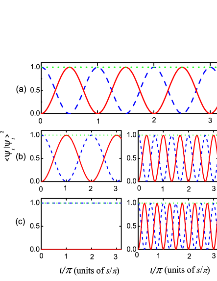
Figure 1: Probability evolution of different values of $\Omega$ for $\gamma=0$: (a) $\Omega=0$; (b) $\Omega=0.5$; (c) $\Omega=1.0$ with the left $\phi/2\pi=0$ and the right $\phi/2\pi=0.5$. Red solid line describes the density of $\left|3\right\rangle$; blue dash line describes the density of $\left|1\right\rangle$; and green dot line is for the total density.

In this paper, we theoretically study the dynamics of the $\mathcal{PT}$ symmetric two-level atoms in three regimes i.e. unbroken $\mathcal{PT}$ symmetry, EP and broken $\mathcal{PT}$ symmetry. The paper is organized as following, we firstly study the time evolution of Hermitian two-level system and then we discuss eigenvalues and investigate dynamics of the effective model with balanced gain and loss. We mainly focus on the effects of Rabi frequency and relative phase. A summary is given. In Supplemental Material the effectively conserved two-level Hamiltonian is derived from the $\Lambda$-type model coupled with two optical fields and one rf field by means of adiabatically eliminating of the third energy level.

I Model of the Two-Level System with $\mathcal{PT}$ symmetry

We consider an effective two-level model with balanced gain and loss. The effective Hamiltonian can be derived from a $\Lambda$-type three-level system via adiabatic elimination of an excited state $\left|2\right\rangle$ under the large detuning condition (see Supplemental Material). The Hamiltonian is described as following:

$$H_{eff} =-i\gamma\left|1\right\rangle\left\langle 1\right|+\left(1-\Omega e^{i\phi}\right)\left|1\right\rangle\left\langle 3\right|$$

$$+i\gamma\left|3\right\rangle\left\langle 3\right|+\left(1-\Omega e^{-i\phi}\right)\left|3\right\rangle\left\langle 1\right|,$$ (1)

where $\left(1-\Omega e^{\pm i\phi}\right)$ describes the effective coupling between states $\left|1\right\rangle$ and $\left|3\right\rangle$, $\Omega$ is the effective strength of a rf field and atom, $\phi$ is the relative phase between rf and two laser fields, and $\gamma$ is the amplitude of gain and loss.

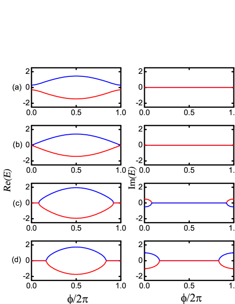
Figure 2: Real (left) and imaginary (right) parts of the eigenvalues of the $\mathcal{PT}$-symmetric two-level system with function of the relative phase $\phi/2\pi$: (a) $\Omega=0.5$, $\gamma=0.4$; (b) $\Omega=0.5$, $\gamma=0.5$; (c) $\Omega=1.0$, $\gamma=0.5$; (d) $\Omega=1.0$, $\gamma=1.0$.

In the absence of $\gamma$, the system is a standard hermitian case. The energy spectrum of the case is two branches, i.e. $E_{\pm}=\pm\sqrt{\left(1-2\Omega\cos\phi+\Omega^{2}\right)}$. For $\Omega<1$, the two branches are well separated by the energy gap. When $\Omega=1$, two branches touch at $\phi=0$. When $\Omega$ is larger than $1$, the energy gap opens again. The dynamics of the Hamiltonian (1) can be obtained by solving the corresponding Schrödinger equation

$$i\partial_{t}\psi=H_{eff}\psi.$$ (2)

Considering the initial condition, $\psi\left(t=0\right)=\psi_{0}$, the dynamic evolution equation can be integrated formally,

$$\psi\left(t\right)=\hat{U}\left(t\right)\psi_{0},$$

where the time evolution operator is defined by $\hat{U}\left(t\right)=\exp\left(-iH_{eff}t\right)$. It can be analytically obtained,

$$\hat{U}\left(t\right)=\left(\begin{array}[]{cc}\cos\left(\omega_{1}t\right)&-i\frac{\left(1-\Omega e^{i\phi}\right)}{\omega_{1}}\sin\left(\omega_{1}t\right)\\ -i\frac{\left(1-\Omega e^{-i\phi}\right)}{\omega_{1}}\sin\left(\omega_{1}t\right)&\cos\left(\omega_{1}t\right)\end{array}\right),$$

where $\omega_{1}=\left|1-\Omega e^{i\phi}\right|$. As a concrete example, we set the initial state as $\psi_{0}=\left(1,0\right)^{T}$. We can obtain the dynamics of both states at time $t$

$$\left|\psi_{1}\left(t\right)\right|^{2} =\frac{1+\cos\left(2\omega_{1}t\right)}{2},$$ (3)

$$\left|\psi_{3}\left(t\right)\right|^{2} =\frac{1-\cos\left(2\omega_{1}t\right)}{2},$$

where $\left|\psi_{1}\left(t\right)\right|^{2}$ $\left(\left|\psi_{3}\left(t\right)\right|^{2}\right)$ is the occupation of $\left|1\right\rangle$ $\left(\left|3\right\rangle\right)$. Fig. 1 shows the probability evolutions of two states for different $\Omega$ following Rabi oscillation with the periodicity $\pi/\omega_{1}$. For $\Omega=0$, $\omega_{1}=1$, only the two-photon term determines the Rabi oscillation as shown in Fig. 1(a). With the increase of $\Omega$ and the relative phase $\phi=0$ (the left column), the periodicity is larger than Fig. 1(a) case. When $\Omega=1$ and $\phi=0$, the Rabi oscillation breaks down. The coexistence of rf-field and two optical fields coherently destructs the oscillation [the left panel of Fig. 1(c)]. However, when $\phi=\pi$ the oscillation periodicity decreases with the increase of $\Omega$ as shown in the right column of Fig. 1(b)-(c). For the hermitian case, we can see the total occupation is always unit and time-independent.

In the present of gain and loss ($\gamma\neq 0$) the eigenvalues of the $\mathcal{PT}$ symmetric Hamiltonian (1) are

$$E_{\pm}=\pm\sqrt{\left|1-\Omega e^{i\phi}\right|^{2}-\gamma^{2}}.$$ (4)

Fig. 2 describes the real and imaginary parts of the eigenvalues of the $\mathcal{PT}$-symmetric two-level system with function of the relative phase $\phi$ for different $\Omega$ and $\gamma$. As shown in Fig. 2(b), when $\gamma=\left|1-\Omega e^{i\phi}\right|$, $E_{+}=E_{-}$ and the eigenvectors coincide, which is defined as the EP $\gamma_{{}_{PT}}$. When $\gamma<\gamma_{{}_{PT}}$, the system has a purely real spectrum and satisfies $\mathcal{PT}$ symmetry [Fig. 2(a)]. Whereas when $\gamma>\gamma_{{}_{PT}}$, the eigenvalues are complex and the symmetry is spontaneously broken [Fig. 2(c)-(d)].

The dynamics of the non-Hermitian two-level quantum system can easily be calculated from the dynamic evolution equation (2). For the Hamiltonian (1) outside the EP, one obtains the evolution operator:

$$\hat{U}\left(t\right)=\left(\begin{array}[]{cc}\cos\left(\omega t\right)-\frac{\gamma}{\omega}\sin\left(\omega t\right)&-i\frac{\left(1-\Omega e^{i\phi}\right)}{\omega}\sin\left(\omega t\right)\\ -i\frac{\left(1-\Omega e^{-i\phi}\right)}{\omega}\sin\left(\omega t\right)&\cos\left(\omega t\right)+\frac{\gamma}{\omega}\sin\left(\omega t\right)\end{array}\right),$$ (5)

with the angular frequency

$$\omega=\sqrt{\left|1-\Omega e^{i\phi}\right|^{2}-\gamma^{2}}.$$ (6)

When $\gamma=0$, $\omega=\omega_{1}$. While, EPs ($\gamma=\gamma_{{}_{PT}}$) are singularities of the spectrum at which spontaneous $\mathcal{PT}$ symmetry breaking has been observed in experiments Ruter . It can lead to some new effects, e.g., chiral behavior and state-exchange process Rabi ; Wunner . Hence, we also focus on the evolution of the system with the parameters approaching EP, i.e., $\omega\rightarrow 0$. In this limit, the time evolution operator is

$$\hat{U}_{EP}\left(t\right)\approx\left(\begin{array}[]{cc}1-\gamma t&-i\left(1-\Omega e^{i\phi}\right)t\\ -i\left(1-\Omega e^{-i\phi}\right)t&1+\gamma t\end{array}\right).$$ (7)

For example, for an initial state $\psi_{0}=\left(1,0\right)^{T}$, we can find outside the EP the norms of two levels are

$$\left|\psi_{1}\left(t\right)\right|^{2} =\left|\cos\left(\omega t\right)-\gamma\frac{\sin\left(\omega t\right)}{\omega}\right|^{2},$$ (8)

$$\left|\psi_{3}\left(t\right)\right|^{2} =\left|i\left(1-\Omega e^{-i\phi}\right)\frac{\sin\left(\omega t\right)}{\omega}\right|^{3},$$

where $\left|\psi_{1,3}\left(t\right)\right|^{2}$ are time-dependent periodic Rabi-type oscillation functions. The period $\pi/\omega$ is dependent on $\gamma$, $\Omega$ and $\phi$, just as the depiction of Eq. (6). In detail Fig. 3 describes some typical cases for the initial state in level $\left|1\right\rangle$. The left column depicts the dynamics for $\phi=0$ and the right column for $\phi=\pi$. Simultaneously, the first two rows, Fig. 3(a) and (b), describe the dynamics of (1) with the same values of $\Omega$ and two different values of $\gamma$ in the $\mathcal{PT}$-symmetric region ($\gamma<\gamma_{{}_{PT}}$), respectively. We can find the envelope amplitudes increase with the increasing of $\gamma$ in column direction. In addition, the corresponding periods of $\phi=0$ are larger than that of $\phi=\pi$. The last row, Fig. 3(c) gives two cases when $\gamma\geqslant\gamma_{{}_{PT}}$. When $\Omega=1$, $\phi=0$ and $\gamma>\gamma_{{}_{PT}}$ (here $\gamma_{{}_{PT}}=0$) due to the coexistence of rf-field and two optical fields coherently destructs only $\left|\psi_{1}\left(t\right)\right|^{2}$ first decreases and then increases to infinity, and meanwhile, $\left|\psi_{3}\left(t\right)\right|^{2}$ is zero all the time as shown in the left panel of Fig. 3(c). In fact in the light of (8) when $\Omega=1$ and $\phi=0$ $\left|\psi_{3}\left(t\right)\right|^{2}$ is always zero whether $\gamma$ is zero or not. When $\gamma=\gamma_{{}_{PT}}$ the wave function evolutes according to the operator (7) and the corresponding norms become

$$\left|\psi_{1}\left(t\right)\right|^{2} =\left|1-\gamma t\right|^{2},$$ (9)

$$\left|\psi_{3}\left(t\right)\right|^{2} =\left|-i\left(1-\Omega e^{-i\phi}\right)t\right|^{2},$$

where $\left|\psi_{1}\left(t\right)\right|^{2}$ first decreases and then increases, and meanwhile, $\left|\psi_{3}\left(t\right)\right|^{2}$ increases for ever as shown in the right panel of Fig. 3(c). In summary, in $\mathcal{PT}$ symmetric region, the time evolution of $\left|\psi_{1,3}\left(t\right)\right|^{2}$ is periodic Rabi-type oscillation and in $\mathcal{PT}$ symmetric broken region the oscillations break down and instead we observe an algebraic growth of the norms.

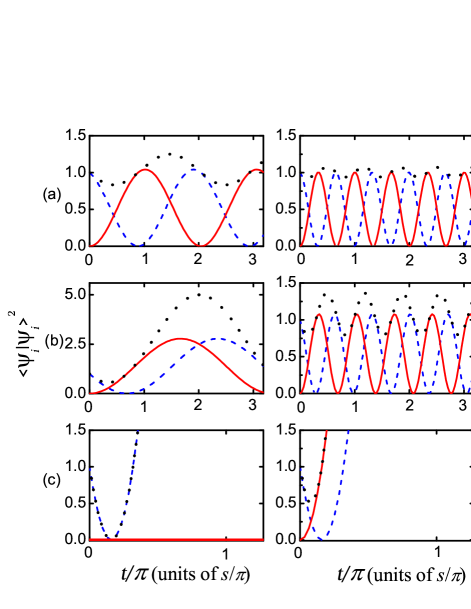
Figure 3: The norm evolutions for Non-Hermitian systems: $\phi=0$ (left) and $\pi$ (right); The first two rows with $\Omega=0.5\$and two different values of $\gamma$: (a) $\gamma=0.1$ and (b) $\gamma=0.4$; The last row (c) $\Omega=1.0$, $\gamma=2.0$. Red solid line describes the norm of $\left|3\right\rangle$, blue dash line is for the norm of $\left|1\right\rangle$, and black dot line is for the total norm.

In order to compare with the Hermitian case, we normalize the total norm. The renormalized state vector Niederle ; Niederle2 can be defined as

$$\varphi_{j}=\frac{\psi_{j}}{\sqrt{\left|\psi_{1}\right|^{2}+\left|\psi_{3}\right|^{2}}},$$ (10)

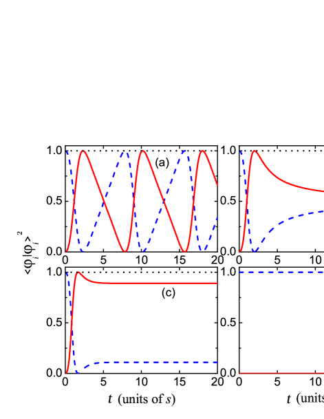
Figure 4: The time evolutions of renormalized states for initial state being $\left(1,0\right)^{T}$ with $\Omega=0.5$ and different values of $\gamma$: (a) $\gamma=0.3$; (b) $\gamma=0.5$; (c) $\gamma=0.8$; And (d) $\gamma=0.1$ and $\Omega=1$. Here $\phi=0$. Red solid line describes for $\varphi_{3}$, blue dash line describes the norm of $\varphi_{1}$, and black dot line is for the time-independent $\left|\varphi_{1}\right|^{2}+\left|\varphi_{3}\right|^{2}$.

which satisfies $\left|\varphi_{1}\right|^{2}+\left|\varphi_{3}\right|^{2}=1$ at any time. Then we start to deal with the time evolution of $\varphi_{j}$ for initial state being $\left(1,0\right)^{T}$. $\left|\varphi_{1,3}\left(t\right)\right|^{2}$ are Rabi-type oscillation in $\mathcal{PT}$ symmetric region [Fig. 4(a)]. The evolution tends towards stability in $\mathcal{PT}$ symmetry broken regime as shown in Figs. 4(b) and 4(c). Fig. 4(d) describes the dynamics similar to the left of Fig. 3(c). To better understand the underlying properties we consider the non-Hermitian effective Schrödinger equation according to the Hamiltonian (1):

$$i\frac{d}{dt}\left(\begin{array}[]{c}\varphi_{1}\\ \varphi_{3}\end{array}\right)=\left(\begin{array}[]{cc}-i\gamma\left(1-\kappa\right)&\left(1-\Omega e^{i\phi}\right)\\ \left(1-\Omega e^{-i\phi}\right)&+i\gamma\left(1+\kappa\right)\end{array}\right)\left(\begin{array}[]{c}\varphi_{1}\\ \varphi_{3}\end{array}\right)$$ (11)

where $\kappa=\left|\varphi_{1}\right|^{2}-\left|\varphi_{3}\right|^{2}$. And further in the familiar way they are translated as the Bloch vectors:

$$s_{x} =\frac{1}{2}\left(\varphi_{1}^{\ast}\varphi_{3}+\varphi_{1}\varphi_{3}^{\ast}\right),$$

$$s_{y} =\frac{1}{2i}\left(\varphi_{1}^{\ast}\varphi_{3}-\varphi_{1}\varphi_{3}^{\ast}\right),$$

$$s_{z} =\frac{1}{2}\left(\varphi_{1}^{\ast}\varphi_{1}-\varphi_{3}^{\ast}\varphi_{3}\right),$$

which are always restricted on the surface of the Bloch sphere and satisfy $s_{x}^{2}+s_{y}^{2}+s_{z}^{2}=1/4$ Niederle . Then we can derive the generalized Bloch equations of motion from Eq. (11):

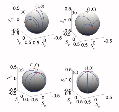
Figure 5: Effective Bloch dynamics with the same parameters as in Fig. 4. Red asterisks (*) embody the initial state vectors of every evolution.

$$\dot{s}_{x} =4\gamma s_{z}s_{x}+2\Omega s_{z}\sin\phi,$$

$$\dot{s}_{y} =4\gamma s_{z}s_{y}-2\left(1-\Omega\cos\phi\right)s_{z},$$

$$\dot{s}_{z} =-\gamma\left(1-4s_{z}^{2}\right)+2s_{y}-2\Omega\left(s_{y}\cos\phi+s_{x}\sin\phi\right).$$ (12)

Thus we can get the effective Bloch dynamical evolution of this non-Hermitian system with different parameters by the fourth-order Runge-Kutta method. Fig. 5 shows some typical examples of the effective Bloch dynamics for different values of $\gamma$, $\Omega$ and $\phi$. When $\gamma<\gamma_{{}_{PT}}$, Fig. 5(a) shows the evolution of arbitrary initial state is the closed circle on the surface of Bloch sphere, which surrounds either of the two fixed points: (i)

$$s_{x}^{0} =\frac{-\Omega\gamma\sin\phi\pm\omega\left(1-\Omega\cos\phi\right)}{2\left(1-2\Omega\cos\phi+\Omega^{2}\right)},$$ (13)

$$s_{y}^{0} =\frac{\gamma\left(1-\Omega\cos\phi\right)\pm\omega\Omega\sin\phi}{2\left(1-2\Omega\cos\phi+\Omega^{2}\right)},$$

$$s_{z}^{0} =0.$$

The fixed points are located in x-y plane. Comparing with the standard model in Niederle , we have more free parameters which is helpful to control dynamics. For example, with the change of $\Omega$ and $\phi$, $s_{y}^{0}$ are not only positive, but also can take negative values. Even in the Hermitian case $\gamma=0$, $s_{y}^{0}$ can take non-zero values due to the phase $\phi$ and $\Omega$. However, at EP, $\gamma=\gamma_{{}_{PT}}$, all initial states would evolute along the corresponding curves and turn back the only one fixed point: (ii)

$$s_{x}^{0} =-\frac{\Omega\sin\phi}{2\gamma},$$ (14)

$$s_{y}^{0} =\frac{\left(1-\Omega\cos\phi\right)}{2\gamma},$$

$$s_{z}^{0} =0,$$

which is still located in x-y plane as shown in Fig. 5(b). It is different from the only result $s_{x}^{0}=0$ mentioned in Niederle . Fig. 5(b) shows the effective Bloch dynamics for $\phi=0$ or $\pi$ where the fixed point $s_{x}^{0}=s_{z}^{0}=0$ and $s_{y}^{0}=1/2$. This helps to investigate the potential character at EP. When $\mathcal{PT}$ symmetry breaks ($\gamma>\gamma_{{}_{PT}}$) there are two fixed points again: (iii)

$$s_{x}^{0} =-\frac{\Omega\sin\phi}{2\gamma},$$ (15)

$$s_{y}^{0} =\frac{\left(1-\Omega\cos\phi\right)}{2\gamma},$$

$$s_{z}^{0} =\pm\frac{\left|\omega\right|}{2\gamma}.$$

The formulas of $s_{x}^{0}$ and $s_{y}^{0}$ are same as (14), however, they decrease with increasing $\gamma$. Compared with (13) and (14) the z axis projections are no longer zero which are labeled as ’$\pm$’. Fig. 5(c) shows any initial states on the Bloch sphere evolutes into one fixed point ($-$), even if initial points are near the other one ($+$). Thus the fixed point ($+$) is defined as a source of the dynamics and the other ($-$) is a sink of the dynamics. Fig. 5(d) describes the dynamics of coherent subtraction, $\Omega=1$ and $\phi=0$, where the fixed points are $s_{x}^{0}=s_{y}^{0}=0$ and $s_{z}^{0}=\pm 1/2$ (correspond to the states: $\left(1,0\right)^{T}$ and $\left(0,1\right)^{T}$). This is the reason that the evolution does not change with time (since the initial state mentioned above is $\left(1,0\right)^{T}$) as shown in the left panel of Figs. 3(c) and 4(d). In addition, the emergence of $s_{z}^{0}$ is the feature of the $\mathcal{PT}$ symmetry breaking. The fixed points are important for the dynamical evolution of $\mathcal{PT}$ symmetry systems.

II Summary

In summary, we consider the effective two-level Hamiltonian with balanced gain and loss. When the system is conserved and Hermitian, the dynamical evolution performs Rabi oscillation and the oscillation periodicity can be controlled by the rf frequency and relative phase. There is one exception at which rf field balance out the actions of two optical fields and oscillation is destructed. For the case of the effective two-level system with $\mathcal{PT}$ symmetry, we study the dynamics in both regions of unbroken and broken $\mathcal{PT}$ symmetry and at EP. Further more, using the renormalized state vector the effective Bloch dynamical evolution has been studied in three conditions. Since the dynamics is closely related to the fixed points, we calculated the solutions under three parameter conditions and found the symmetry breaks when the z component of the fixed points is not zero, meanwhile the projection in x-y plane can be fully adjusted by the phase and strength of optical and rf fields. It shall be helpful to the implementation of related experiment.

This work is supported by the NSF of China under Grants No.11104171, 11404199, 11574187 and the Youth Science Foundation of Shanxi Province of China under Grant No. 2012021003-1. Z. Xu is supported by the NSF of Chian under Grants No. 11604188, NSF for youths of Shanxi Province No. 201601D201027 and 1331KSC.

References

- (1) Bender C M and Boettcher S 1998 Phys. Rev. Lett. 80 5243; Bender C M, Boettcher S, and Meisinger P N 1999 J. Math. Phys. 40 2201.
- (2) Guo A, Salamo G J, Duchesne D, Morandotti R, Volatier-Ravat M, Aimez V, Siviloglou G A and Christodoulides D N 2009 Phys. Rev. Lett. 103 093902.
- (3) Rüter C E, Makris K G, EI-Ganainy R, Christodoulides D N, Segev M and Kip D 2010 Nature Phys. 6 192.
- (4) Bittner S, Dietz B, Günther U, Harney H L, Miski-Oglu M, Richter A and Schäfer F 2012 Phys. Rev. Lett. 108 024101.
- (5) Chang L, Jiang X, Hua S, Yang C, Wen J, Jiang L, Li G, Wang G, and Xiao M 2014 Nature Photon. 8 524.
- (6) Feng L, Wong Z J, Ma R-M, Wang Y, and Zhang X 2014 Science 346 972.
- (7) Hodaei H, Miri M A, Heinrich M, Christodoulides D N, and Khajavikhan M 2014 Science 346 975.
- (8) Hodaei H, Miri M A, Hassan A U, Hayenga W E, Heinrich M, Christodoulides D N, and Khajavikhan M 2015 Opt. Lett. 40 4955.
- (9) Schindler J, Lie A, Zheng M C, Ellis F M and Kottos T 2011 Phys. Rev. A 84 040101.
- (10) Peng B, Ozdemir S K, Lei F, Monifi F, Gianfreda M, Long G L, Fan S, Nori F, Bender C M, and Yang L 2014 Nature Phys. 10 394; Jing H, Özdemir S K, Geng Z, Zhang J, Lü X -Y, Peng B, Yang L and Nori F 2015 Science Report 5 9663.
- (11) Wimmer M, Miri M -A, Christodoulides D and Peschel U 2015 Science Report 5 17760.
- (12) Ben-Aryeh Y, Mann A and Yaakov I 2004 J. Phys. A: Math. Gen. 37 12059.
- (13) Bender C M, Brody D C, Jones H F, and Meister B K 2007 Phys. Rev. Lett. 98 040403.
- (14) Graefe E -M 2012 J. Phys. A: Math. Theor. 45 444015.
- (15) Lian X, Zhong H, Xie Q, Zhou X, Wu Y and Liao W 2014 Eur. Phys. J. D. 68 189.
- (16) Baradaran M and Panahi H 2017 Chin. Phys. B, 26 060301.
- (17) Graefe E-M, Korsch H J, and Niederle A E 2008 Phys. Rev. Lett 101 150408.
- (18) Graefe E-M, Korsch H J, and Niederle A E 2010 Phys. Rev. A 82 013629.
- (19) Zhu B, Lü R, and Chen S 2015 Phys. Rev. A 91 042131; 2016 Phys. Rev. A 93 032129.
- (20) Jin L and Song Z 2009 Phys. Rev. A 80 052107; Yuce C 2015 Phys. Lett. A 379 1213; Joglekar Y N, Scott D, Babbey M, and Saxena A 2010 Phys. Rev. A 82 030103(R).
- (21) Bergmann K, Theuer H, and Shore B W 1998 Rev. Mod. Phys. 70 1003.
- (22) Alexanian M and Bose S K 1995 Phys. Rev. A 52 2218.
- (23) Sun X-L, Zhang J-W, Cheng P-F, Zuo Y-N, and Wang L-J 2018 Chin. Phys. B 27 023101.
- (24) Shahriar M S and Hemmer P R 1990 Phys. Rev. Lett. 65 1865.
- (25) Li H, Sautenkov V A, Rostovtsev Y V, Welch G R, Hemmer P R, and Scully M O 2009 Phys. Rev. A 80 023820.
- (26) Luo B, Tang H and Guo H 2009 J. Phys. B: At. Mol. Opt. Phys. 42 235505.
- (27) Basler C, Grzesiak J, and Helm H 2015 Phys. Rev. A 92 013809.
- (28) Novikov S, Sweeney T, Robinson J E, Premaratne S P, Suri B, Wellstood F C, and Palmer B S 2016 Nature Phys. 12 75.
- (29) Peng P, Cao W, Shen C, Qu W, Wen J, Jiang L and Xiao Y 2016 Nature Phys. 12 1139.
- (30) Bender C M, Brody D C, and Jones H F 2002 Phys. Rev. Lett. 89 270401.
- (31) Milburn T J, Doppler J, Holmes C A, Portolan S, Rotter S, and Rabl P 2015 Phys. Rev. A 92 052124.
- (32) Menke H, Klett M, Cartarius H, Main J, and Wunner G 2016 Phys. Rev. A 93 013401.
- (33) Hang C, Huang G, and Konotop V V 2013 Phys. Rev. Lett. 110 083604.
- (34) Li H, Dou J, and Huang G 2013 Opt. Express 21 32053.
- (35) Lee T E and Chan C-K 2014 Phys. Rev. X. 4, 041001.
- (36) Hao Y and Gu Q 2011 Phys. Rev. A 83 043620.