Dynamical evolutions in non-Hermitian triple-well system with complex potential

Abstract

We investigate the dynamical properties for non-Hermitian triple-well system with a loss in the middle well. When chemical potentials in two end wells are uniform and nonlinear interactions are neglected, there always exists a dark state, whose eigenenergy becomes zero, and the projections onto which do not change over time and the loss factor. The increasing of loss factor only makes the damping form from the oscillating decay to over-damping decay. However, when the nonlinear interaction is introduced, even interactions in the two end wells are also uniform, the projection of the dark state will be obviously diminished. Simultaneously the increasing of loss factor will also aggravate the loss. In this process the interaction in the middle well plays no role. When two chemical potentials or interactions in two end wells are not uniform all disappear with time. In addition, when we extend the triple-well system to a general $(2n+1)$-well, the loss is reduced greatly by the factor $1/2n$ in the absence of the nonlinear interaction.

LABEL:FirstPage1 LABEL:LastPage#16

I Introduction

In quantum mechanical pictures Hamiltonian must be Hermitian to describe a physical system, which is sufficient to ensure that the system has real energy eigenvalues and the conservation of the number of particles. But this condition is too rigorous in real systems. In optics, a non-Hermitian Hamiltonian is used to describe the propagation of light in the medium with complex refraction index Moiseyev ; Longhi ; Kivshar ; Luo1 ; Musslimani ; Kottos . Recently the controlled removal of atoms from a Bose-Einstein condensate (BEC) can be realized by a narrow electron beam or a narrow laser beam Ott ; Konotop , which promotes simulations of the atomic system with dissipation. The systems with dissipation process are described via the non-Hermitian Hamiltonians with negative imaginary chemical potential Bender ; Bender2 ; Mostafazadeh ; Chen ; Wunner ; Niederle ; Livi ; Ng ; Konotop1 and can be solved in terms of the master equations Zoller ; Zoller2 ; Cirac ; Wimberger ; Altman ; Ciuti ; Lee . More importantly, in most cases dissipation is considered as an undesirable destructing factor, thus people make arduous efforts to avoid it at all if possible, such as inverting the dissipation by means of an intrinsic mechanism to balance the losses Konotop ; Rotter ; Wunner1 , probing a quantum system with controlled dissipation Ivana , and designing the effective dissipative process in an optical superlattice using the coupling between the system and the reservoir Zoller , etc. Massive efforts have been invested in the study of the dynamics of non-Hermitian systems in experiment and theory Zoller ; Greiner ; Bloch ; Lee2 ; Cao .

The study of few-well systems reveals a variety of interesting quantum phenomena. For example, condensates in double or three wells have popularly been investigated both theoretically and experimentally Gati ; Smerzi1 ; LiuJie1 ; LiuJie2 ; Oberthaler1 ; Oberthaler2 ; Oberthaler3 ; Levy ; Smerzi2 ; Smerzi ; Shore ; zhu ; fu ; Munro . In past years nonlinear Josephson oscillation and self-trapping phenomena are two of many important findings for double wells. However, more attentions have been focused on three-well system Shore ; zhu ; fu ; Munro , which has more abundant physical picture by adjusting the tunneling and interaction parameters, as well as chemical potentials. For example, under periodic driving of this model coherent destruction of tunneling and dark Floquet state have been predicted in theory Luo . Thus, dark states can also be controlled and realized in the three-state (three-well) system. Even chaotic phenomena and bifurcation mechanism causing self-trapping have been studied in the dynamics of three coupled condensate systems Penna ; Penna2 . In addition, in the light propagation in waveguides, the Kerr nonlinear interactions induce a variety of interesting quantum phenomena Scully . Thus when dissipation and the nonlinear interaction together play the roles in triple-well system, novel features may be expected in the dynamical evolution of the system.

In the present paper, we mainly study the quantum dynamics of a non-Hermitian triple-well system. We focus on the time evolutions of modulus squared of coefficients in three local states without nonlinear interactions. The analytic solutions of the Schrödinger equations directly give the time-dependent information for uniform chemical potentials in two end wells. The finding is that the eigenstate is a dark state, whose eigenergy is zero, the projection on which is not dependent of time and the loss factor. But when chemical potentials in two ends are not uniform, the dark state would be not any more the eigenstate. Moreover, when nonlinear terms in three wells are considered, the modulus squared in three wells will be quickly diminished. These results are still suitable for systems of odd wells with similar structure.

II Model and analytic solutions in linear case

We consider a coupled triple-well system with an imaginary chemical potential in the middle well. In general, the wave function $\left|\psi\left(t\right)\right\rangle$ of the system is a superposition of states at three local sites, i.e.,

$$\left|\psi\left(t\right)\right\rangle=c_{1}\left(t\right)\left|1\right\rangle+c_{2}\left(t\right)\left|2\right\rangle+c_{3}\left(t\right)\left|3\right\rangle,$$ (1)

where $c_{i}(t)$ are the amplitudes for three states $\left|i\right\rangle$ ($i=1,2,3$). In this local site space, where the spatial dependence of the states will not be considered, the dynamic equation of the system Livi ; Ng ; Konotop1 reads ($\hbar=1$)

$$i\frac{\partial}{\partial t}\left(\begin{array}[]{c}c_{1}\\ c_{2}\\ c_{3}\end{array}\right)=H\left(\begin{array}[]{c}c_{1}\\ c_{2}\\ c_{3}\end{array}\right)$$ (2)

with the Hamiltonian

$$H=\left(\begin{array}[]{ccc}\mu_{1}+g_{1}\left|c_{1}\right|^{2}&-J&0\\ -J&\mu_{2}+g_{2}\left|c_{2}\right|^{2}&-J\\ 0&-J&\mu_{3}+g_{3}\left|c_{3}\right|^{2}\end{array}\right).$$ (3)

The chemical potentials $\mu_{1}$ and $\mu_{3}$ are real and $\mu_{2}=\eta-i\alpha$ is a complex number, which denotes an effective loss ($\alpha>0$) or a gain ($\alpha<0$) at the state $\left|2\right\rangle$ Wunner ; Niederle . $g_{i}$ is the strength of the Kerr nonlinearity in state $\left|i\right\rangle$ and $J$ is the coupling strength Kottos2 . We set $J=1$ so that all energies are in units of $J$.

We first focus on the simplest case that the chemical potentials are symmetrically distributed ($\mu_{1}=\mu_{3}$), and the interactions are neglected $g_{i}=0$. The Schrödinger equation (2) can be solved by a substitution $c_{i}\left(t\right)=c_{i}^{0}\exp\left(-i\lambda_{i}t\right)$ and one has the eigenvalues $\lambda_{i}$ for Hamiltonian (3)

$$\lambda_{1} =\mu_{1},$$

$$\lambda_{2,3} =\frac{1}{2}\left(\mu_{1}+\mu_{2}\pm\Theta\right),$$ (4)

and the corresponding ket space is spanned by three eigenvectors

$$\left|\psi_{1}\right\rangle=\left(\begin{array}[]{c}-1\\ 0\\ 1\end{array}\right),\left|\psi_{2}\right\rangle=\left(\begin{array}[]{c}1\\ \lambda_{3}-\mu_{2}\\ 1\end{array}\right),\left|\psi_{3}\right\rangle=\left(\begin{array}[]{c}1\\ \lambda_{2}-\mu_{2}\\ 1\end{array}\right),$$ (5)

where $\Theta=\sqrt{\left(\mu_{1}-\mu_{2}\right)^{2}+8}$. We do not bother to normalize them because the normalization factor will not affect the final result. The dual, bra space with eigenvector, e.g., $\left\langle\psi_{2}\right|=(1,\lambda_{3}^{\ast}-\mu_{2}^{\ast},1)$ is not orthogonal to the ket space. It is thus necessary to define the Hilbert space of $H^{\dagger}$, $\left|\tilde{\psi}_{i}\right\rangle=\left|\psi_{i}^{\ast}\right\rangle$, the bra vectors being $\left\langle\tilde{\psi}_{i}\right|=\left\langle\psi_{i}^{\ast}\right|$. Here the symbol $\ast$ means the complex conjugate for all complex numbers. These eigenvectors together form a biorthogonal basis, i.e. the completeness relation reads Heiss

$$\sum_{k}\frac{\left|\psi_{k}\right\rangle\left\langle\tilde{\psi}_{k}\right|}{\left\langle\tilde{\psi}_{k}|\psi_{k}\right\rangle}=1,$$ (6)

and the orthogonality means

$$\frac{\left\langle\psi_{k}|\tilde{\psi}_{k^{\prime}}\right\rangle}{\left\langle\psi_{k}|\tilde{\psi}_{k}\right\rangle}=\delta_{kk^{\prime}}.$$ (7)

Note that the eigenvector $\psi_{1}$ is a dark state which is the superposition of two local states in the left and right wells. The completeness dictates that an arbitrary normalized initial state $\left|\psi\left(0\right)\right\rangle=\left(c_{1}^{0},c_{2}^{0},c_{3}^{0}\right)^{T}$ can be expressed in the eigenvector space (5)

$$\left|\psi\left(0\right)\right\rangle=A_{1}\left|\psi_{1}\right\rangle+A_{2}\left|\psi_{2}\right\rangle+A_{3}\left|\psi_{3}\right\rangle,$$ (8)

where the coefficients $A_{i}$ are suitable combinations of $c_{i}^{0}$, for example, $A_{1}=\left(c_{3}^{0}-c_{1}^{0}\right)/\sqrt{2}$ for a normalized $\left|\psi_{1}\right\rangle$. At time $t$ the wave function evolves according to

$$\left|\psi\left(t\right)\right\rangle=A_{1}e^{-i\lambda_{1}t}\left|\psi_{1}\right\rangle+A_{2}e^{-i\lambda_{2}t}\left|\psi_{2}\right\rangle+A_{3}e^{-i\lambda_{3}t}\left|\psi_{3}\right\rangle.$$ (9)

The matrix for the time evolution operator $C$ in the local site space defined as Konotop

$$\left|\psi\left(t\right)\right\rangle=\left(\begin{array}[]{ccc}C_{11}\left(t\right)&C_{12}\left(t\right)&C_{13}\left(t\right)\\ C_{21}\left(t\right)&C_{22}\left(t\right)&C_{23}\left(t\right)\\ C_{31}\left(t\right)&C_{32}\left(t\right)&C_{33}\left(t\right)\end{array}\right)\left|\psi\left(0\right)\right\rangle,$$ (10)

can be calculated as

$$C=S^{\dagger}Diag\left(e^{-i\lambda_{1}t},e^{-i\lambda_{2}t},e^{-i\lambda_{3}t}\right)\tilde{S}$$ (11)

where $S$ is transformation matrix between the site space and the eigenvector space with the adjoint matrix $\tilde{S}$. These operators are necessarily not unitary. Actually, formed by merging the eigenvectors $|\psi_{i}\rangle$ or $\left|\tilde{\psi}_{i}\right\rangle$ into a square matrix row by row, the operators $S^{\dagger}$ and ${\tilde{S}}^{\dagger}$ satisfy $S^{\dagger}{\tilde{S}}={\tilde{S}}S^{\dagger}=1$ and ${\tilde{S}}^{\dagger}S=S{\tilde{S}}^{\dagger}=1$. In this way, the time-dependent matrix elements $C_{ij}\left(t\right)$ in eq. (10) can be determined as

$$C_{11}\left(t\right) =C_{33}\left(t\right)=\frac{1}{2}e^{-i\lambda_{1}t}+\frac{1}{2}f_{+}\left(t\right),$$

$$C_{31}\left(t\right) =C_{13}\left(t\right)=-\frac{1}{2}e^{-i\lambda_{1}t}+\frac{1}{2}f_{+}\left(t\right),$$

$$C_{22}\left(t\right) =f_{-}\left(t\right),$$

$$C_{12}\left(t\right) =C_{21}\left(t\right)=C_{23}\left(t\right)=C_{32}\left(t\right)$$

$$=\frac{1}{\Theta}\left(e^{-i\lambda_{3}t}-e^{-i\lambda_{2}t}\right),$$ (12)

where

$$f_{+}\left(t\right) =\frac{\lambda_{2}-\mu_{2}}{\Theta}e^{-i\lambda_{2}t}-\frac{\lambda_{3}-\mu_{2}}{\Theta}e^{-i\lambda_{3}t},$$

$$f_{-}\left(t\right) =\frac{\lambda_{2}-\mu_{2}}{\Theta}e^{-i\lambda_{3}t}-\frac{\lambda_{3}-\mu_{2}}{\Theta}e^{-i\lambda_{2}t}.$$ (13)

The symmetry in the coefficients $C_{ij}$ reflects directly that of the Hamiltonian in the local site space. For an arbitrary initial state $\left|\psi\left(0\right)\right\rangle$, we can infer the state evolution $\left|\psi\left(t\right)\right\rangle$ by the coefficients $C_{ij}\left(t\right)$, i.e. the amplitude on the $i$-th local state reads $c_{i}\left(t\right)=C_{i1}\left(t\right)c_{1}^{0}+C_{i2}\left(t\right)c_{2}^{0}+C_{i3}\left(t\right)c_{3}^{0}$. Correspondingly the modulus squared of coefficient in each local state are

$$P_{i}\left(t\right)=\left|c_{i}\left(t\right)\right|^{2},$$ (14)

and the sum is

$$P_{all}\left(t\right)=\sum_{i}P_{i}\left(t\right).$$ (15)

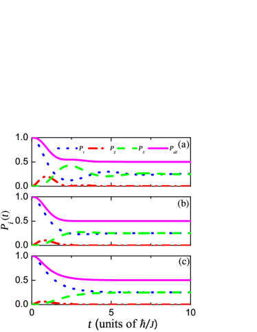
Figure 1: Time evolution of the modulus squared of coefficient in each well $P_{i}(t)$ and the sum $P_{all}$ (pink solid line) with the loss factor $\alpha=1$ (a), $\alpha=2$ (b) and $\alpha=3$ (c) starting from the initial state $c_{1}^{0}=1$, $c_{2}^{0}=c_{3}^{0}=0$. Here $\mu_{1}=\mu_{3}=\eta=0$.

For simplicity now we assume that the chemical potentials in left and right states vanish and that in local state $\left|2\right\rangle$ is pure imaginary, i.e. $\mu_{1}=\mu_{3}=0$ and $\mu_{2}=-i\alpha$. We focus on the case of dissipation in the rest of the paper, i.e., $\alpha>0$. It is easy to see that while $\Theta$ in the eigenvalues $\lambda_{2,3}$ is positive and real for $\alpha^{2}<8$, it becomes pure imaginary for $\alpha^{2}>8$. This will greatly change the time dependence of the functions $f_{\pm}$. When $\alpha^{2}<8$, we see $\Theta=\left|\Theta\right|$ and the functions $f_{\pm}\left(t\right)$ reduces to

$$f_{\pm}\left(t\right)=\pm e^{-\frac{1}{2}\alpha t}\frac{\sin\left(\frac{1}{2}\left|\Theta\right|t\pm\beta\right)}{\sin\beta},$$ (16)

where $\beta=\arcsin\left(\left|\Theta\right|/\sqrt{8}\right)$. Due to the sinusoidal functions in Eq. (16), it describes an oscillating decay process starting from $f_{\pm}(0)=1$. We find the critical damping occurs at $\alpha^{2}=8$. In the other case when $\alpha^{2}>8$, $\Theta=i\left|\Theta\right|$, the system enters the over-damping region

$$f_{\pm}\left(t\right)=\pm e^{-\frac{1}{2}\alpha t}\frac{\sinh\left(\frac{1}{2}\left|\Theta\right|t\pm\beta^{\prime}\right)}{\sinh\beta^{\prime}},$$ (17)

where $\beta^{\prime}=\text{arcsinh}\left(\left|\Theta\right|/\sqrt{8}\right)$. Since $\left|\alpha\right|>\left|\Theta\right|$, the decaying term $e^{-\alpha t/2}$ of $f_{+}\left(t\right)$ in Eq. (17) will be compensated by the monotonically increasing hyperbolic sine function, which leads to over-damping, i.e. a relatively slow decay compared with Eq.(16) in the chemical parameter region $\alpha^{2}<8$. As an example, starting from the initial state $c_{1}^{0}=1$ and $c_{2}^{0}=c_{3}^{0}=0$, the distributions in three states are respectively

$$P_{1}\left(t\right) =\left|C_{11}\left(t\right)\right|^{2}=\frac{1}{4}\left|f_{+}\left(t\right)+1\right|^{2},$$

$$P_{3}\left(t\right) =\left|C_{31}\left(t\right)\right|^{2}=\frac{1}{4}\left|f_{+}\left(t\right)-1\right|^{2},$$ (18)

and

$$P_{2}\left(t\right) =\left|C_{21}\left(t\right)\right|^{2}$$

$$=\frac{2}{\left|\Theta\right|^{2}}e^{-\alpha t}\left\{\begin{array}[]{c}1-\cos\left(\left|\Theta\right|t\right),\qquad\alpha^{2}<8,\\ \cosh\left(\left|\Theta\right|t\right)-1,\qquad\alpha^{2}>8.\end{array}\right.$$ (21)

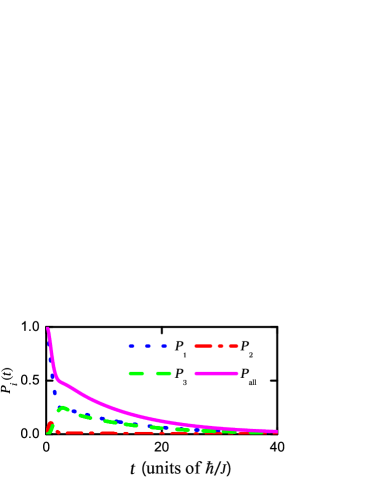
Figure 2: Time evolution of the modulus squared of coefficient in each well $P_{i}(t)$ and the sum $P_{all}$ (pink solid line) for non-equal distribution of the chemical potentials starting from the initial state $c_{1}^{0}=1$, $c_{2}^{0}=c_{3}^{0}=0$. Here $\mu_{1}=0.1$, $\mu_{3}=0.5$ and $\alpha=2$.

The time evolution of the modes are shown in Fig. 1 for three different values of $\alpha$. For $\alpha=1$, we find $P_{1}\left(t\right)$ and $P_{3}\left(t\right)$ undergo explicit oscillations around the same equilibrium value $0.25$. These modulus squared values return rapidly to their equilibrium value for $\alpha=2$, with an obvious damping oscillation. For $\alpha=3$, however, the decrease of $P_{1}\left(t\right)$ and the increase of $P_{3}\left(t\right)$ are much slower, which shows the typical behavior of over-damping. In both cases $P_{2}\left(t\right)$ quickly oscillates to a vanishingly small value, which means the leakage of the mode from the middle well. In addition we find the equilibrium values for $P_{i}$ in the limit $t\rightarrow+\infty$ are independent of $\alpha$. In this limit $e^{-i\lambda_{2,3}t}\rightarrow 0$ and $f_{\pm}\left(t\right)\rightarrow 0$, for arbitrary initial state the wave function $\left|\psi\left(t\right)\right\rangle$ reduces to

$$\left|\psi\left(t\rightarrow+\infty\right)\right\rangle=\frac{c_{3}^{0}-c_{1}^{0}}{2}\left(\begin{array}[]{c}-1\\ 0\\ 1\end{array}\right),$$ (22)

and the associated norms are

$$P_{1,3}\left(t\rightarrow+\infty\right) =\frac{\left(c_{1}^{0}-c_{3}^{0}\right)^{2}}{4},\qquad$$

$$P_{2}\left(t\rightarrow+\infty\right) =0.$$ (23)

This indicates that the steady state is the dark state $\left|\psi_{1}\right\rangle$, the projection on which would be stored forever. For the initial state $c_{1}^{0}=1$ and $c_{2}^{0}=c_{3}^{0}=0$, it is easy to show that the total norm $P_{all}\left(t\rightarrow+\infty\right)=0.5$, which does not vary with $\alpha$ as depicted in Fig. 1. These results show apparent suppression of dissipation because the projection on the dark state does not change with time. Similar things happen for other initial states, even for the dark state $\psi_{1}$ itself Bender2 ; Baker ; Graefe ; Hao .

The linear non-Hermitian system with non-zero chemical potentials can be solved readily by $\left|\psi\left(t\right)\right\rangle=\exp\left(-iHt\right)\left|\psi\left(0\right)\right\rangle$ and the three modulus squared parameters $P_{i}$ are given by (14). For non-equal chemical potentials in the left and right wells $\mu_{1}\neq\mu_{3}$, the dark state $\left|\psi_{1}\right\rangle$ is not any more the eigenstate of the system Dark . An immediate result is that $P_{i}$ in all three states will be lost in the limit $t\rightarrow+\infty$. We show this full leakage in Fig. 2 for $\alpha=2$, $\mu_{1}=0.1$ and $\mu_{3}=0.5$. Clearly, the probability $P_{1}=1$ in the initial state $(1,0,0)^{T}$ decays from $1$ to $0$, at the same time $P_{2,3}$ reduce to zero after a temporary increase.

Under the balanced condition $\mu_{1}=\mu_{3}$, it is interesting to study the influence of the real part $\eta$ of $\mu_{2}$ on the evolution of each state. As an example, we set $\mu_{1}=\mu_{3}=0.5$ and $\alpha=2$ and increase the real part $\eta$ from $0$ to $6$. The modulus squared $P_{1,3}$ are found to oscillate in longer and longer time, which effectively slows down the process for the sum of $P_{i}$ to reach the equilibrium. However, it has no effect on the distribution of the steady state in the limit $t\rightarrow+\infty$.

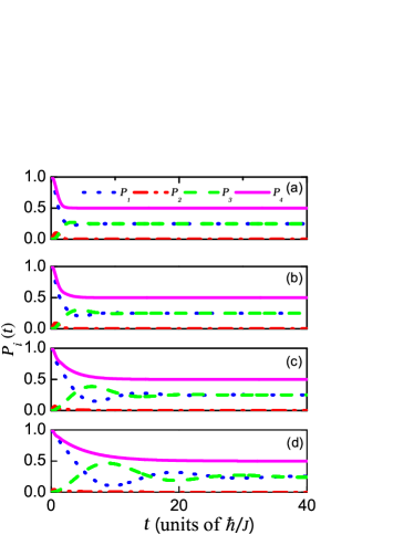
Figure 3: The effect of the real part of $\mu_{2}$ on the evolution of $P_{i}\left(t\right)$ with $\eta=0$ (a), $2$ (b), $4$ (c) and $6$ (d). Here $\mu_{1}=\mu_{3}=0.5$ and $\alpha=2$.

III Numerical Scheme for nonlinear interaction case

The analytical solution in above section is not available when the nonlinear interaction is introduced in the Hamiltonian (3). In looking for the similar variational ansatz solution (1), we need to take several approximations into account: (a) First of all, the time evolution of the wave function (1) is described as the superposition of three local states Smerzi . The nonlinear terms in the dynamic equations (2), on the other hand, would destroy such a superposition. When the probability in the tunneling region of the adjacent wells is small enough such that the nonlinear interaction in these regions is negligible, the superposition ansatz (1) is applicable. (b) In the meantime we decompose the time and the spatial dependence of the wave function $\left|\psi\left(t\right)\right\rangle$, which has been verified numerically in the study of BEC trapped in double well potential PHD . (c) The spatial dependence of the local states will not be considered here, despite that the overlap of the states determines the tunneling strength $J$ and the interaction parameters $g_{i}$ Malomed1 . To investigate the dynamics of the system with nonlinear terms, we deal with the time-dependent Hamiltonian in the site space by means of the successive iteration, i.e. starting from an arbitrarily normalized initial state $\left|\psi\left(0\right)\right\rangle$, the wave function at time $t+\delta t$ is evolved from previous time $t$ through

$$\left|\psi\left(t+\delta t\right)\right\rangle=\exp\left(-iH[t]\delta t\right)\left|\psi\left(t\right)\right\rangle,$$ (24)

while the time-dependence of the Hamiltonian $H[t]$ is described by the interaction terms $\left|c_{i}\left(t\right)\right|^{2}$ in equation (3). Accordingly, we numerically split the evolution time $t$ into many small intervals with the time step $\delta t$ being small enough to admit a solution with good precision. We note that unlike in the case of time-dependent Gross-Pitaevskii equations for dissipative BEC in double well Hao or the barrier transmission of BEC in waveguide Graefe , the absence of the kinetic term makes it much easier for the convergence of the solution.

We now discuss the typical numerical results with different nonlinear parameters. For nonzero interaction existing only in the middle well $g_{1}=g_{3}=0$ and $g_{2}=3$, the stationary solutions for different loss $\alpha=1$ and $3$ are shown in Fig. (4a) and (4b). The stationary solutions are identical to results of noninteracting case in Fig. (1b) and (1c), which shows that $g_{2}$ does not affect the evolution of $P_{i}\left(t\right)$ in limit $t\rightarrow\infty$. For three identical interaction parameters $g_{1}=g_{3}=g_{2}=3$, on the other hand, we observe quite different behavior. The nonlinear terms $g_{1,3}$ obviously diminish the projection of the dark state to a very low level, and moreover $P_{i}$ also decrease with the increase of $\alpha$. Unequal $g_{1}\neq g_{3}$ would destroy the coherent character completely, leading to a full leakage of the wave-packet.

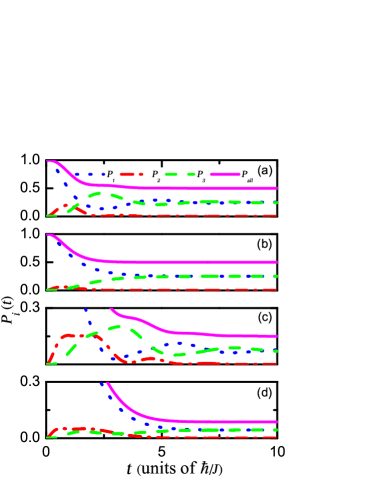
Figure 4: A numerical investigation of evolutions for different nonlinear parameters: When $g_{1}=g_{3}=0$, $g_{2}=3$, $\alpha=1$ (a) and $3$ (b); When $g_{1}=g_{3}=g_{2}=3$, $\alpha=1$ (c) and $3$ (d). Here $\mu_{1}=\mu_{3}=0$ and initial conditions: $c_{1}^{0}=1$ and $c_{2}^{0}=c_{3}^{0}=0$.

IV Generalization to any odd site number

We have dealt with the three-well model with a loss in the middle site and found there is a dark state when $\mu_{1}=\mu_{3}$ and $g_{i}=0$. Then based on this we also discussed the time evolution for different parameters and even different interactions. These results can be generalized to a general $(2n+1)$-well system where only the middle site has a loss and is coupled with other wells. For simplicity, firstly we consider the five-well model. The Hamiltonian is

$$H_{5}=\left(\begin{array}[]{ccccc}\mu_{1}&0&-1&0&0\\ 0&\mu_{2}&-1&0&0\\ -1&-1&\mu_{3}&-1&-1\\ 0&0&-1&\mu_{4}&0\\ 0&0&-1&0&\mu_{5}\end{array}\right)$$ (25)

where $\mu_{3}=-i\alpha$ and $\mu_{i\neq 3}=0$ and only $\left|3\right\rangle$ is coupled with the rest of wells. When dealing with $\left|H_{5}-EI\right|=0$, we can obtain

$$E^{3}\left(E^{2}+i\alpha E-4\right)=0.$$

For eigen energy $E=0$, we can get

$$c_{3} = 0,$$

$$c_{1}+c_{2}+c_{4}+c_{5} = 0,$$ (26)

where $c_{i}$ are the coefficients of $\left|i\right\rangle$. The solutions of (26) are not unique and correspond to triplet dark states with a node structure in the middle well and other coefficients summed up to zero. Hence we analyze the dynamics of this model by the numerical method, just as the section. III in this paper. But from (26) we can find that the eigenvectors with $E=0$ have not projection in $\left|3\right\rangle$ because of $c_{3}=0$, which is independent of any parameter. So the projection in these eigenvectors would not vary over time. In order to further explain it, using numerical method (24) we can find when $\left|\psi\left(0\right)\right\rangle=\left(1,0,0,0,0\right)^{T}$,

$$\lim_{t\rightarrow\infty}P_{all}\left(t\right)=3/4,$$

which is the projection in the eigenvectors with $E=0$ and is much larger than in three-well system as shown in Fig. 5. Accordingly, we study an arbitrary $(2n+1)$-well system, and set $\mu_{n+1}=-i\alpha$ and $\mu_{j\neq n+1}=0$. With the same numerical method we find the law: $\lim_{t\rightarrow\infty}P_{all}\left(t\right)=1-1/2n$ with $\left|\psi\left(0\right)\right\rangle=\left(1,0,0,\cdots,0\right)^{T}$, which coincides the above-mentioned results. This gives a good application that more wells may be used to construct sophisticated dark states, the projection onto which is kept on a much higher level in the steady state of dynamical evolution.

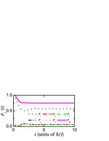
Figure 5: Time evolutions of modulus squared of coefficients in five wells for initial states $\left|1,0,0,0,0\right\rangle$. Here nonlinear terms $g_{i}=0$ and the loss factor $\alpha=2$.

V Conclusions

We have presented a detailed analysis of dynamical evolutions of the three-well system with a loss in the middle well. When the chemical potentials in two end wells are real and uniform, there is always a dark state, the projection on which does not change over time and the loss factor $\alpha$. But there exists a critical value, where the norms at two end sites evolute from damping oscillation to over-damping. When the chemical potentials in two end wells are not uniform, the dark state is not any more the eigenstate of the system and three norms will decay to zero. In addition, when the nonlinear interactions are introduced and uniform in two end wells, the projection of dark state will be obviously diminished, but do not disappear. And the projection also decrease with the increase of the loss factor. However, the interaction at middle site plays no role and the dark state is proven to be the key to the suppression of the dissipation. In addition, the other two interaction intensities would promote the loss. When extending the triple-well system to a general $(2n+1)$-well we found that the total norm follows the law $1-1/2n$ in the absent of interactions, which can be used to enhance the anti-leakage capability in signal propagation in certain medium with dissipation.

This work is supported by the NSF of China under Grants No.11574187, 11674201, 11474189, 11425419 and 11374354.

References

- (1) S. Klaiman, U. Günther, and N. Moiseyev, Phys. Rev. Lett. 101, 080402 (2008).
- (2) S. Longhi, Phys. Rev. Lett. 103, 123601 (2009).
- (3) A. A. Sukhorukov, Z. Xu, and Y. S. Kivshar, Phys. Rev. A 82, 043818 (2010).
- (4) X. Luo, J. H. Huang, H. H. Zhong, X. Z. Qin, Q. T. Xie, Y. S. Kivshar, and C. H. Lee, Phys. Rev. Lett. 110, 243902 (2013).
- (5) Z. H. Musslimani, K. G. Makris, R. El-Ganainy, and D. N. Christodoulides, Phys. Rev. Lett. 100, 030402 (2008).
- (6) H. Ramezani, D. N. Christodoulides, V. Kovanis, I. Vitebskiy, and T. Kottos, Phys. Rev. Lett. 109, 033902 (2012).
- (7) T. Gericke, C. Utfeld, N. Hommerstad, and H. Ott, Las. Phys. Lett. 3, 415 (2006); T. Gericke, P.Würtz, D. Reitz, T. Langen, and H. Ott, Nat. Phys. 4, 949 (2008).
- (8) V. S. Shchesnovich and V. V. Konotop, Phys. Rev. A 81, 053611 (2010).
- (9) C. M. Bender and S. Boettcher, Phys. Rev. Lett. 80, 5243 (1998); C. M. Bender, D. C. Brody and H. F. Jones, Phys. Rev. Lett. 89, 270401 (2002).
- (10) C. M. Bender, Rep. Prog. Phys. 70, 947 (2007).
- (11) A. Mostafazadeh and A. Batal, J. Phys. A 37, 11645 (2004).
- (12) B. Zhu, R. Lü and S. Chen, Phys. Rev. A 89, 062102 (2014).
- (13) D. Dast, D. Haag, H. Cartarius, and Güter Wunner, Phys. Rev. A 90. 052120 (2014).
- (14) E. M. Graefe, H. J. Korsch, and A. E. Niederle, Phys. Rev. Lett. 101, 150408 (2008), Phys. Rev. A 82, 013629 (2010).
- (15) R. Livi, R. Franzosi, and G.-L. Oppo, Phys. Rev. Lett. 97, 060401(2006).
- (16) G. S. Ng, H. Hennig, R. Fleischmann, T. Kottos, and T. Geisel, New J. Phys. 11, 073045 (2009).
- (17) V. A. Brazhnyi, V. V. Konotop, V. M. Perez-Garcia, and H. Ott, Phys. Rev. Lett. 102, 144101 (2009).
- (18) S. Diehl, A. Micheli, A. Kantian, B. Kraus, H. P. Büchler and P. Zoller, Nat. Phys. 4, 878 (2008).
- (19) S. Diehl, A. Tomadin, A. Micheli, R. Fazio, and P. Zoller, Phys. Rev. Lett. 105, 015702 (2010); A. Tomadin, S. Diehl, and P. Zoller, Phys. Rev. A 83, 013611 (2011).
- (20) F. Verstraete, M. M. Wolf, and J. Ignacio Cirac, Nat. Phys. 5, 633 (2009).
- (21) D. Witthaut, F. Trimborn, and S. Wimberger, Phys. Rev. Lett. 101, 200402 (2008).
- (22) E. G. Dalla Torre, E. Demler, T. Giamarchi, and E. Altman, Nat. Phys. 6, 806 (2010).
- (23) A. Le Boité, G. Orso, and C. Ciuti, Phys. Rev. Lett. 110, 233601 (2013).
- (24) T. E. Lee and C.-K. Chan, Phys. Rev. X. 4, 041001 (2014).
- (25) J. Doppler, A. A. Mailybaev, J. Böhm, U. Kuhl, A. Girschik, F. Libisch, T. J. Milburn,P. Rabl, N. Moiseyev and S. Rotter, Nature 537, 76 (2016).
- (26) W. D. Heiss and G. Wunner, Eur. Phys. J. D 71, 312 (2017).
- (27) I. Vidanovic, D. Cocks, and W. Hofsterter, Phys. Rev. A 89, 053614 (2014).
- (28) W. S. Bakr, J. I. Gillen, A. Peng, S. Fölling, and M. Greiner, Nature (London) 462, 74 (2009).
- (29) J. F. Sherson, C. Weitenberg, M. Endres, M. Cheneau, I. Bloch, and S. Kuhr, Nature (London) 467, 68 (2010).
- (30) T. E. Lee, F. Reiter, and N. Moiseyev, Phys. Rev. Lett. 113, 250401 (2014).
- (31) H. Cao and J. Wiersig, Rev. Mod. Phys. 87, 61 (2015).
- (32) R. Gati, M. K. Oberthaler, J. Phys. B 40, R61 (2007).
- (33) F.S. Cataliotti, S. Burger, C. Fort, P. Maddaloni, F. Minardi, A. Trombettoni, A. Smerzi, M. Inguscio, Science 293, 843 (2001).
- (34) T. Anker, M. Albiez, R. Gati, S. Hunsmann, B. Eiermann, A. Trombettoni, M.K. Oberthaler. Phys. Rev. Lett. 94, 020403 (2005).
- (35) Jie Liu, Libin Fu, Bi-Yiao Ou, Shi-Gang Chen, Dae-Il Choi, Biao Wu, and Qian Niu, Phys. Rev. A 66, 023404 (2002).
- (36) Guan-Fang Wang, Di-Fa Ye, Li-Bin Fu, Xu-Zong Chen, and Jie Liu, Phys. Rev. A 74,033414 (2006).
- (37) M. Albiez, R. Gati, J. Foelling, S. Hunsmann, M. Cristiani, M. K. Oberthaler, Phys. Rev. Lett. 95, 010402 (2005).
- (38) T. Zibold, E. Nicklas, C. Gross, M. K. Oberthaler, Phys. Rev. Lett. 105, 204101 (2010).
- (39) S. Levy, E. Lahoud, I. Shomroni, J. Steinhauer, Nature 449, 579 (2007).
- (40) L. J. LeBlanc, A.B. Bardon, J. McKeever, M.H.T. Extavour, D. Jervis, J.H. Thywissen, F. Piazza, A. Smerzi, Phys. Rev. Lett. 106, 025302 (2011).
- (41) A. Smerzi, S. Fantoni, S. Giovanazzi, and S. R. Shenoy, Phys. Rev. Lett. 79, 4950 (1997); G. J. Milburn, J. Corney, E. M. Wright, and D. F. Walls, Phys. Rev. A 55, 4318 (1997); S. Raghavan, A. Smerzi, S. Fantoni, and S. R. Shenoy, Phys. Rev. A 59, 620 (1999).
- (42) K. Bergmann, H. Theuer and B. W. Shore, Rev. Mod. Phys. 70 1003 (1998).
- (43) Y. Du, Z. Liang, W. Huang, H. Yan, and S. Zhu, Phys. Rev. A 90, 023821 (2014). M. Semczuk, W. Gunton, W. Bowden, and K. W. Madison, Phys. Rev. Lett. 113, 055302 (2014).
- (44) B. Liu, L. Fu, S. Yang and J. Liu, Phys. Rev. A 75, 033601 (2007).
- (45) K. Nemoto, C. A. Holmes, G. J. Milburn, and W. J. Munro, Phys. Rev. A 63, 013604 (2000).
- (46) X. Luo, L. Li, L. You and B. Wu, New J. Phys. 16 013007 (2014).
- (47) R. Franzosi and V. Penna, Phys. Rev. A 65, 013601 (2001).
- (48) R. Franzosi and V. Penna, Phys. Rev. E 67, 046227 (2003).
- (49) M. O. Scully and M. S. Zubairy, Quantum Optics, Cambridge University Press, Cambridge (1996).
- (50) H. Ramezani and T. Kottos, Phys. Rev. A 82, 043803 (2010).
- (51) W. D. Heiss, and H. L. Harney, Eur. Phys. J. D 17, 149 (2001).
- (52) N. Moiseyev and L. S. Cederbaum, Phys. Rev. A 72, 033605 (2005).
- (53) P. Schlagheck and T. Paul, Phys. Rev. A 73, 023619 (2006); K. Rapedius and H. J. Korsch, ibid. 77, 063610 (2008); J. Phys. B 42, 044005 (2009).
- (54) E.-M. Graefe, H. J. Korsch, and A. E. Niederle, Phys. Rev. A 82, 013629 (2010); H. Zheng, Y. Hao and Q. Gu, J. Phys. B: At. Mol. Opt. Phys. 46 065301 (2013).
- (55) K. Bergmann, H. Theuer, and B. W. Shore, Rev. Mod. Phys. 70 1003 (1998); B. Luo, H. Tang and H. Guo, J. Phys. B: At. Mol. Opt. Phys.. 42, 235505 (2009).
- (56) S. Giovanazzi, Ph.D. thesis, SISSA-ISAS, 1998 (unpublished).
- (57) E.-M. Graefe, J. Phys. A: Math. Theor. 45, 444015 (2012); X. Zhang, J. Chai, J. Huang, Z. Chen, Y. Li, and B. A. Malomed, Opt. Exp. 22, No. 11, 13927-13939 (2014); Z. Chen, J. Huang, J. Chai, X. Zhang, Y. Li, and B. A. Malomed, Phys. Rev. A 91, 053821 (2015).