A-Optimal Sampling and Robust Reconstruction for Graph Signals via Truncated Neumann Series
Fen Wang, Yongchao Wang, Member, IEEE, and Gene Cheung, Senior Member, IEEE The research of F. Wang and Y. Wang was supported in part by National Science Foundation of
China under grant 61771356, 111 project of China under grant B08038.F. Wang and Y. Wang are with State Key Lab. of ISN, School
of Telecom. Engineering, Xidian University, No.2 Taibai South Road,
Xi’an, 710071, Shaanxi, China.(Email:ychwang@mail.xidian.edu.cn).G. Cheung is with National Institute of Informatics, 2-1-2, Hitotsubashi, Chiyoda-ku, Tokyo, 101-8430, Japan. (Email:cheung@nii.ac.jp).
Abstract
Graph signal processing (GSP) studies signals that live on irregular data kernels described by graphs.
One fundamental problem in GSP is sampling—from which subset of graph nodes to collect samples in order to reconstruct a bandlimited graph signal in high fidelity.
In this paper, we seek a sampling strategy that minimizes the mean square error (MSE) of the reconstructed bandlimited graph signals assuming an independent and identically distributed (iid) noise model—leading naturally to the A-optimal design criterion.
To avoid matrix inversion, we first prove that the inverse of the information matrix in the A-optimal criterion is equivalent to a Neumann matrix series.
We then transform the truncated Neumann series based sampling problem into an equivalent expression that replaces eigenvectors of the Laplacian operator with a sub-matrix of an ideal low-pass graph filter.
Finally, we approximate the ideal filter using a Chebyshev matrix polynomial.
We design a greedy algorithm to iteratively minimize the simplified objective.
For signal reconstruction, we propose an accompanied signal reconstruction strategy that reuses the approximated filter sub-matrix and is provably more robust than conventional least square recovery.
Simulation results show that our sampling strategy outperforms two previous strategies in MSE performance at comparable complexity.
Index Terms:
Graph signal processing (GSP), sampling, optimal design.
I Introduction
Graph signal processing (GSP) is the study of discrete signals that live on irregular data kernels described by graphs [1, 2].
One fundamental problem in GSP is sample selection—optimally select a subset of graph nodes from which to collect samples such that an assumed bandlimited signal can be reconstructed in high fidelity111Sampling can also be done via aggregation [7]: observe the same signal after different graph shifts but only at one node.[3, 4, 5, 6].
Under noiseless conditions, [8] proved that a qualified sampling set that leads to perfect signal reconstruction requires only full column rank of a sampling matrix, and empirically showed that it can be accomplished with high probability via random node selection for a connected graph via large experiments.
Random node selection can result in a poor condition number in the reconstruction matrix, however.
In response, authors in [9, 10, 11] proposed an efficient sampling strategy based on spectral proxies that selects stable nodes for unique reconstruction without full eigen-decomposition.
If the observed samples are corrupted by noise, [12] adopts an E-optimality criterion for sampling, which minimizes the worst case reconstruction error.
However, most graph sampling works222[5] proposed a generic greedy procedure, termed as minimum Frobenius norm (MFN) based selection, to minimize the A-optimality criterion but no fast algorithms. We compare against [5] in our experiments. do not adopt and optimize a minimum mean square error (MMSE) objective directly, which leads naturally to an A-optimality design criterion assuming an independent and identically distributed (iid) additive noise model [13].
Beyond the fact that graph sampling is inherently combinatorial in nature, one main difficulty lies in the computation of the inverse of an information matrix, which in general has complexity .
While [14] showed that greedy methods optimizing the A-optimality criterion can have near-optimal performance, no efficient implementation was proposed, which in general requires eigen-decomposition and/or inversion of large matrices.
In this letter, we propose a computation-efficient graph sampling strategy that addresses the A-optimality criterion directly.
We first prove that the inverse information matrix in the A-optimality criterion is equivalent to a Neumann matrix series.
We next transform the truncated Neumann series based sampling problem into an equivalent expression that replaces eigenvectors of the Laplacian operator with a sub-matrix of an ideal graph low-pass filter [1, 10].
Finally, we approximate the low-pass filter with a Chebyshev matrix polynomial [15]—arriving at a simplified proxy that approximates the A-optimality objective but requires neither full eigen-decomposition nor matrix inversion.
We propose a greedy algorithm to minimize the simplified objective.
For signal reconstruction, we design an accompanied reconstruction strategy that is provably more “robust” 333By “robustness”, we mean resilience of an estimator’s presumably good MSE performance for small noise as noise variance increases. to large noise than the least square (LS) solution while reusing the earlier computed approximate low-pass filter sub-matrix.
Experimental results show that our A-optimality based sampling strategy outperforms previous schemes in MSE at comparable complexity.
II Signal Processing on Graphs
Denote by a graph containing a set of nodes indexed by .
is the set of weighted edges.
An edge weight reflects the similarity between nodes and .
In this letter, we focus on connected, undirected graphs with no multiple edges and adopt the symmetric normalized Laplacian matrix as the variation operator, where and .
Assuming that the eigen-decomposition of is where with , and , then the graph Fourier transform (GFT) of a graph signal is defined as and the inverse GFT is .
A graph signal is called bandlimited if there exists a number such that [12].
The smallest such is called the bandwidth of .
Graph signals with bandwidth at most are called -bandlimited (-BL) graph signals, which are expressed as
.
means the first columns of and denotes the first elements of .
Definition 1[16]: In order to select elements from to produce with and , we define the sampling matrix as
(1)
where is the set of sampling indices, means the -th element of set , and is the number of elements in .
denotes the complement set of .
is the number of edges.
For any matrix , we adopt the notation to denote the sub-matrix of with rows indexed by and columns indexed by .
is simplified to .
is the identity matrix whose dimension depends on the context.
III Sample Selection for Noisy -BL Graph Signals
A sampled -BL graph signal can now be written as .
In noiseless condition, can be perfectly recovered from when , using the LS solution [12]:
(2)
where means the pseudo-inverse operator.
When corrupted by noise, a sampled -BL graph signal is .
Using (2) as the recovery method, we get an estimator .
Assuming that noise is iid with zero mean and unit variance, the covariance matrix of the reconstruction error is
[11].
By the theory of optimal experiments design [17], minimizing the trace of the covariance matrix leads to the known A-optimality criterion:
(3)
Notice that the A-optimality criterion coincides with the MMSE criterion.
An alternative criterion is to minimize the largest eigenvalue of —as adopted in [12]—known as the E-optimality criterion, which minimizes the worst case signal reconstruction.
Unlike [12], we address directly the MMSE criterion in (3) to achieve smallest signal reconstruction error on average, but doing so without any matrix inversion or eigen-decomposition, where complexity is in general.
III-AMatrix Inversion Approximation
Proposition 1: The inverse matrix in (3) exists and is equivalent to its Neumann series, i.e.,
(4)
if the selected matrix is full column rank, i.e.,
(5)
Proof: For simplicity, we denote , and let be the eigenvalues of .
The Neumann series theorem [18, Section 5.6] states that if , then the Neumann series will converge to , which exactly implies (4).
From the definition of , under appropriate permutation.
Hence, and ,
(6)
where .
Since , .
Because , is positive definite, which results in and .
Based on the Rayleigh quotient theorem [18], and .
As discussed in [12], (5) is the definition of qualified sampling operators, and it is ensured with high probability via random node selection when .
The necessary condition for a qualified sampling operator is thus , which is the focus region of all sampling strategies.
In the following analysis, we assume that (5) is satisfied.
We propose the following sampling method by substituting the inverse matrix in (3) with a truncated Neumann series.
(7)
where is a truncation parameter.
Proposition 2:
When is approximated by its truncated Neumann series, the estimation error between (3) and (7) is
(8)
See Appendix A in the supporting document for the proof of this result.
Equation (8) implies that the proper design of depends on the sizes of which are influenced by the sampling strategy, sampling size and .
Larger would result in a smaller truncation error.
In this letter, we set and show that its estimate error is reasonably small in Section V.
Leveraging on a property of the trace operator, we further transform (7) into an equivalent problem that involves an ideal low-pass graph filter with cutoff frequency .
Theorem 1: The sampling problem (7) is equivalent to
(9)
where is an ideal low-pass graph filter (implementation to be discussed in details) and the relationship between and is defined in (1).
Proof: Denote by .
Because and , .
As a result,
(10)
where means the binomial coefficients and is derived from the property of trace operation.
Since under appropriate permutation, .
Hence, ,
which will lead to
(11)
where “” denotes a nonzero matrix whose dimension is .
Therefore, .
Combined with (10), where and are constant during sampling, which implies Theorem 1.
TABLE I: Outline of The Proposed MIA Sampling Algorithm
Input:
, bandwidth , sample size and truncation parameter
Output:
Sampling set
Step 1.
, compute of
Step 2.
Calculate the truncated Chebyshev polynomial approximation of and then compute
Step 3.
While
end
Step 4.
Return and
III-BChebyshev Approximation of Low-pass Filter
The low-pass graph filter has a kernel function .
We approximate this spectral kernel function via Chebyshev polynomial approximation [15], after which can be expressed by a matrix polynomial in terms of , i.e., [19].
Finally, the sampling problem is formulated as
(12)
If we solve (7) directly, the eigenvector matrix of dimension is required.
After transforming (7) to (12), the required information is only .
We compute as follows.
We first compute an -by- tridiagonal matrix using the Lanczos algorithm, which preserves of [20].
For a large sparse graph, the complexity of the Lanczos algorithm is .
We then compute the eigenvalues of the tridiagonal matrix using a fast multipole method, whose complexity is [21]. Hence, the combined complexity for computing is , where .
Along with , the computation of may be done only once during preparation, and implemented efficiently due to the sparsity of .
III-CComplexity Analysis
Optimizing the proposed criterion (12) is still combinatorial, so we adopt a greedy algorithm to obtain its solution, which we call the matrix inversion approximation (MIA) sampling algorithm.
Details of the algorithm are presented in Table I.
The complexity for computing is .
Calculating the coefficients and has complexity and [15].
Hence, in the preparation step, the complexity of MIA is .
In each sampling step, the algorithm involves matrix multiplication, where and gradually increases until , having an asymptotic complexity of [22].
Considering the impact from and , the complexity of each search step is .
Since finally , the whole complexity of the sampling step is .
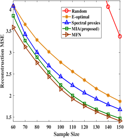
((a))Reconstruction MSE in G1 at 10dB
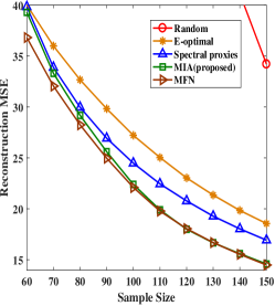
((b))Reconstruction MSE in G1 at 0dB
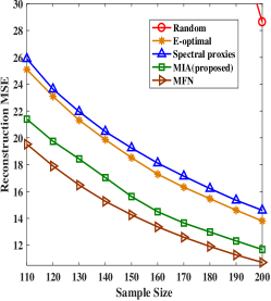
((c))Reconstruction MSE in G2 at 0dB
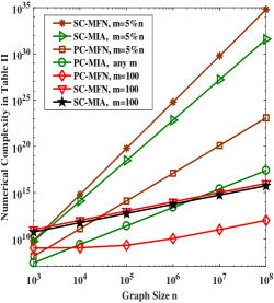
((d))Complexity comparison
Figure 1: (a) (b) (c) Simulation results for different sampling algorithms where graph signals are all recovered by the LS reconstruction, (d) Numerical comparison of complexity between the MFN and the MIA algorithms where “PC” and “SC” are the abbreviation of the complexity of the preparation step and that of the sampling step respectively.
TABLE II: Complexity Comparison of Different Sampling Strategies
Preparation
Selection step
Spectral Proxies
NONE
E-optimal
MFN
MIA
Table II compares the computational complexity among different sampling strategies, in which we assume and adopt some results in [11].
In the preparation step, the spectral proxies algorithm utilizes directly, while is necessary for the E-optimal and the MFN algorithms.
In the selection step, the E-optimal and the MFN algorithms need singular value decomposition and the first eigen-pair of is required for the spectral proxies algorithm.
IV Accompanied Reconstruction Strategy
Assuming , then according to Proposition 1, the LS solution of a graph signal is equivalent to
(13)
It is easy to derive that
(14)
where holds since
.
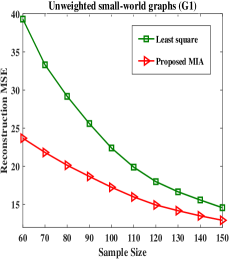
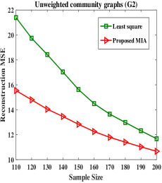
Figure 2: Reconstruction MSE for different reconstruction algorithms in G1 and G2 at 0dB where the sampling algorithm are all the MIA sampling.
Combining (11), (IV) and (IV), a closed-form reconstruction strategy (named as MIA reconstruction) is given by
(19)
(22)
where and .
and have been computed in Table I, so the MIA recovery strategy only needs matrix-vector product, thus has low complexity.
Moreover, assuming the Chebyshev polynomial approximates the ideal low-pass filter well enough, this proposed MIA reconstruction method is more robust to large noise than the LS reconstruction in theory.
See Appendix B in the supporting document for the proof of the robustness.
V Experimental Results
We evaluated our proposed strategy via simulations.
All experiments were performed in MATLAB R2017b, running on a PC with Intel Core I3 3.7 GHz CPU and 16GB RAM.
Artificial graphs:(G1) Small-world graphs [23] (unweighted) with 1000 nodes, degree 8 and connection probability 0.1; (G2) Community graphs [24] (unweighted) with 1000 nodes.
Artificial signals: The true signal is exactly bandlimited with and the non-zero GFT coefficients are generated from .
Samples are corrupted by AWGN.
Other Parameters: We set for the MIA algorithm and for the spectral proxies algorithm.
In the complexity comparison experiments, we set , and .
The SGWT toolbox [24] is adopted to approximate the ideal low pass filter, where and [10].
Fig. 1(a), (b) and (c) show that our proposed MIA sampling algorithm achieves better MSE performance than the E-optimal and spectral proxies algorithms and closely approximates the performance of the MFN algorithm in both small-world graphs and community graphs at different SNRs.
Fig.1 (d) shows that although the complexity of the MIA algorithm for the preparation step may be larger for a constant , when is a fixed percentage of , the proposed MIA algorithm has smaller complexity for both the preparation step and the sampling step compared to the MFN algorithm, especially for large graphs.
To evaluate the Neumann truncation error at , we computed the ratio between the estimate error in (8) and the MSE value in (3) in small-world graphs.
Numerical results reveal that when , this ratio was 0.19.
We also performed simulations using our proposed MIA reconstruction method, where the sample sets were all collected by the MIA sampling algorithm.
As depicted in Fig. 2, the MIA reconstruction outperformed the LS reconstruction in both small-world graphs and community graphs at 0dB.
These results empirically validate the robustness of the proposed MIA reconstruction algorithm for large noise variance.
Acknowledgments
The authors would like to thank Dr. Aamir Anis, Dr. Xuan Xue and the anonymous reviewers for constructive comments that led to improvements in the manuscript.
References
[1]
D. Shuman, S. Narang, P. Frossard, A. Ortega, and P. Vandergheynst, “The emerging field of signal processing on graphs: Extending high-dimensional data analysis to networks and other irregular domains,” IEEE Signal Process. Mag., vol. 30, no. 3, pp. 83-98, May. 2013.
[2]
A. Sandryhaila and J. Moura, “Big data analysis with signal processing
on graphs: Representation and processing of massive data sets with irregular structure,” IEEE Signal Process. Mag., vol. 31, no. 5, pp. 80-90,
Sep. 2014.
[3]
I. Pesenson, “Sampling in Paley-Wiener spaces on combinatorial
graphs,” Trans. Amer. Math. Soc., vol. 360, no. 10, pp. 5603-5627,
2008.
[4]
G. Puy, N. Tremblay, R. Gribonval, and P. Vandergheynst, “Random sampling of bandlimited signals on graphs,” Appl. Comput. Harmon. Anal., 2016.
[5]
M. Tsitsvero, S. Barbarossa, and P. Di Lorenzo, “Signals on graphs: Uncertainty principle and sampling,” IEEE Trans. Signal Process., vol. 64, no. 18, pp. 4845-4860, Sept.15, 2016.
[6]
F. Gama, A. G. Marques, G. Mateos, and A. Ribeiro, “Rethinking sketching as sampling:
A graph signal processing approach,” arXiv preprint , arXiv:1611.00119, 2016.
[7]
A. Marques, S. Segarra, G. Leus, and A. Ribeiro,“Sampling of graph
signals with successive local aggregations,” IEEE Trans. Signal Process.,
vol. 64, no. 7, pp. 1832-1843, 2016.
[8]
I. Shomorony and A. Avestimehr, “Sampling large data on graphs,” in
Proc. IEEE Global Conf. Signal Inf. Process. (GlobalSIP), pp. 933-936, Dec. 2014.
[9]
A. Anis, A. Gadde, and A. Ortega, “Towards a sampling theorem
for signals on arbitrary graphs,” in Proc. IEEE Int. Conf. Acoust.,
Speech, Signal Process. (ICASSP), Florence, Italy, pp. 3864-3868,
May. 2014.
[10]
A. Gadde, A. Anis, and A. Ortega, “Active semi-supervised learning using sampling theory for graph signals,” in Proc. 20th ACM SIGKDD Int. Conf.
Knowl. Discov. Data Min., pp. 492-501, 2014.
[11]
A. Anis, A. Gadde, and A. Ortega, “Efficient sampling set selection for
bandlimited graph signals using graph spectral proxies,” IEEE Trans.
Signal Process., vol. 64, no. 14, pp. 3775-3789, Jul. 2016.
[12]
S. Chen, R. Varma, A. Sandryhaila, and J. Kovačević, “Discrete signal
processing on graphs: Sampling theory,” IEEE Trans. Signal Process.,
vol. 63, no. 24, pp. 6510-6523, 2015.
[13]
S. Boyd and L. Vandenberghe, Convex Optimization, Cambridge University Press, 2004.
[14]
L. F. O. Chamon and A. Ribeiro, “Greedy sampling of graph signals,” IEEE Trans. Signal Process., vol. 66, no. 1, pp. 34-47, Jan.1, 2018.
[15]
D. Hammond, P. Vandergheynst, and R. Gribonval, “Wavelets on graphs via spectral graph theory,” Appl. Comput. Harmon. Anal., vol. 30, no. 2, pp. 129-150, 2011.
[16]
S. Chen, A. Sandryhaila, and J. Kovačević, “Sampling theory for graph signals,” in Proc. IEEE Int. Conf. Acoust., Speech, Signal Process. (ICASSP), South Brisbane, Queensland, Australia, pp. 3392-3396,
Apr. 2015.
[17]
F. Pukelsheim, Optimal Design of Experiments. Philadelphia, PA, USA: SIAM, 1993, vol. 50.
[18]
R. A. Horn and C. R. Johnson, Matrix Analysis. Cambridge University Press, 2013.
[19]
S. K. Narang, A. Gadde, E. Sanou, and A. Ortega, “Localized iterative methods for interpolation in graph structured data,” in Proc. IEEE Global Conf. Signal Inf. Process. (GlobalSIP), Austin,USA, pp. 491-494, 2013.
[20]
G. Golub and C. F. V. Loan, Matrix Computations (Johns Hopkins Studies in the Mathematical Sciences). Johns Hopkins University Press, 2012.
[21]
E. S. Coakley and V. Rokhlin, “A fast divide-and-conquer algorithm for computing the spectra of real symmetric tridiagonal matrices,” Appl. Comput. Harmon. Anal., 2013.
[22]
V. V. Williams, “Multiplying matrices in time,” Stanford University, July 1, 2014.
[23]
D. J. Watts and S. H. Strogatz, “Collective dynamics of small-world networks,” Nature, vol. 393, no. 6684, pp. 440-442,
1998.
[24]
N. Perraudin, J. Paratte, D. Shuman, V. Kalofolias, P. Vandergheynst, and D. K. Hammond, “GSPBOX: A toolbox for signal processing on graphs,”
Aug. 2014, arXiv:1408.5781 [cs.IT].
APPENDIX
A. Proof of Proposition 1
Assuming that the eigen-decomposition of is
where and .
Then,
where , is the -th eigenvalue of and has been proved in Proposition 1.
Therefore,
(23)
where denotes the -th eigenvalue of a matrix.
As a result,
B. Proof of the robustness of the MIA reconstruction
Assume that the graph signal has the same energy for different SNR, i.e., is a constant matrix, and the distribution of noise is iid with zero mean and variance which varies with SNR.
A corrupted -BL graph signal is .
1) Least square (LS) reconstruction
If original signal is recovered by the LS reconstruction method, i.e.,
According to Proposition 1 in our paper, the above LS reconstruction is equivalent to
If an original signal is recovered by the proposed MIA method, i.e., truncating the first items of the infinite matrix polynomial,
where is a vector representing the Von Neumann series truncation error on the bandlimited signal itself, that remains constant for different noise variance.
Then, the corresponding MSE of the MIA reconstruction is
Combining (25), (28) and (29), we can see that when noise variance, i.e., , is very large, the proposed MIA reconstruction method will achieve better MSE performance.
Thus, we can safely claim that our proposed reconstruction method is more robust to large noise than the LS reconstruction.