Joint Estimation and Inference for Data Integration Problems based on Multiple Multi-layered Gaussian Graphical Models

Abstract

The rapid development of high-throughput technologies has enabled the generation of data from biological or disease processes that span multiple layers, like genomic, proteomic or metabolomic data, and further pertain to multiple sources, like disease subtypes or experimental conditions. In this work, we propose a general statistical framework based on Gaussian graphical models for horizontal (i.e. across conditions or subtypes) and vertical (i.e. across different layers containing data on molecular compartments) integration of information in such datasets. We start with decomposing the multi-layer problem into a series of two-layer problems. For each two-layer problem, we model the outcomes at a node in the lower layer as dependent on those of other nodes in that layer, as well as all nodes in the upper layer. We use a combination of neighborhood selection and group-penalized regression to obtain sparse estimates of all model parameters. Following this, we develop a debiasing technique and asymptotic distributions of inter-layer directed edge weights that utilize already computed neighborhood selection coefficients for nodes in the upper layer. Subsequently, we establish global and simultaneous testing procedures for these edge weights. Performance of the proposed methodology is evaluated on synthetic and real data.

Keywords: Data integration; Gaussian Graphical Models; neighborhood selection; group lasso; high-dimensional asymptotics; multiple testing; false discovery rate

1 Introduction

Aberrations in complex biological systems develop in the background of diverse genetic and environmental factors and are associated with multiple complex molecular events. These include changes in the genome, transcriptome, proteome and metabolome, as well as epigenetic effects. Advances in high-throughput profiling techniques have enabled a systematic and comprehensive exploration of the genetic and epigenetic basis of various diseases, including cancer (Lee et al., 2016; Kaushik et al., 2016), diabetes (Yuan et al., 2014; Sas et al., 2018), chronic kidney disease (Atzler et al., 2014), etc. Further, such multi-Omics collections have become available for patients belonging to different, but related disease subtypes, with The Cancer Genome Atlas (TCGA: Tomczak et al. (2015)) being a prototypical one. Hence, there is an increasing need for models that can integrate such complex data both vertically across multiple modalities and horizontally across different disease subtypes.

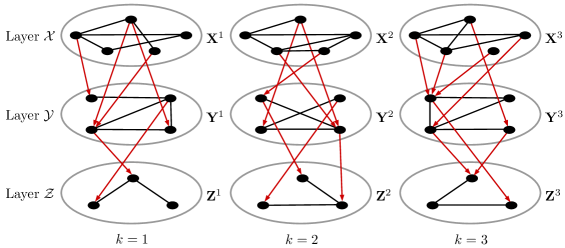
Figure 1: Multiple multilayer graphical models. The matrices $({\mathbf{X}}^{k},{\mathbf{Y}}^{k},{\mathbf{Z}}^{k}),k=1,2,3$ indicate data for each layer and category $k$. Within-layer connections (black lines) are undirected, while between-layer connections (red lines) go from an upper layer to the successive lower layer. For each type of edges (i.e. within ${\cal{X}},{\cal{Y}},{\cal{Z}}$ and ${\cal{X}}\rightarrow{\cal{Y}},{\cal{Y}}\rightarrow{\cal{Z}}$), there are common edges across some or all $k$.

Figure 1 provides a schematic representation of the horizontal and vertical structure of such heterogeneous multi-modal Omics data as outlined above. A simultaneous analysis of all components in this complex layered structure has been coined in the literature as data integration. While it is common knowledge that this will result in a more comprehensive picture of the regulatory mechanisms behind diseases, phenotypes and biological processes in general, there is a dearth of rigorous methodologies that satisfactorily tackle all challenges that stem from attempts to perform data integration (Joyce and Palsson, 2006; Gomez-Cabrero et al., 2014; Gligorijević and Pržulj, 2015). A review of the present approaches towards achieving this goal, which are based mostly on specific case studies, can be found in Gligorijević and Pržulj (2015) and Zhang et al. (2017).

Contributions

of this paper are two-fold. Firstly, we propose an integrative framework to conduct simultaneous inference for all parameters in multiple and multi-layer graphical models, essentially formalizing the structure in Figure 1. We decompose the multi-layer problem into a series of two-layer problems, propose an estimation algorithm for them based on group penalization, and derive theoretical properties of the estimators. Generalizing to group structures on the model parameters allows us to incorporate prior information, as and when available, on within-layer or between-layer sub-graph components shared across some or all $k=1,\cdots,K$. For biological processes, such information can stem from experimental or mechanistic knowledge (for example a pathway-based grouping of genes). Secondly, we obtain debiased versions of within-layer regression coefficients in this two-layer model, and derive their asymptotic distributions using estimates of model parameters that satisfy generic convergence guarantees. Subsequently, we formulate a global test, as well as a simultaneous testing procedure that controls for False Discovery Rate (FDR) to detect important pairwise differences among directed edges between layers.

The novel techniques developed are based on a small number of technical assumptions that are quite general. For example, the model quantities used in our global testing procedure do not necessarily need to be sparse, and instead are only required to have $O(\sqrt{\text{parameter dimension}/n})$ finite sample error bounds that have become standard in the high-dimensional literature (for example see Loh and Wainwright (2012); Basu and Michailidis (2015); Basu et al. (2019)). The advantage of this fiexibility is that components can be switched out to adapt the framework to other technical assumptions. The optional group sparsity assumptions in our estimation technique can be replaced by other structural restrictions (or no restrictions), for example low-rank or low-rank-plus-sparse, as deemed appropriate by the prior dependency assumptions across parameters. As long as these resulting estimates converge to the true parameters at the specified finite-sample rates, they can be used by the developed testing methodology.

Related work

Gaussian Graphical Models (GGM) have been extensively used to model biological networks in the last few years. While the initial work on GGMs focused on estimating undirected edges within a single network through obtaining sparse estimates of the inverse covariance matrix from high-dimensional data (e.g. see references in Bühlmann and van de Geer (2011)), attention has shifted to estimating parameters from more complex structures. This includes (1) analyzing multiple related but not identical graphical models simultaneously, and (2) stacking up more multiple graphical models to form hierarchical multilayer networks, with both directed and undirected edges. For the first class of problems, Guo et al. (2011) and Xie et al. (2016) assumed perturbations over a common underlying structure to model multiple precision matrices, while Danaher et al. (2014) proposed using fused/group lasso type penalties for the same task. To incorporate prior information on the group structures across several graphs, Ma and Michailidis (2016) proposed the Joint Structural Estimation Method (JSEM), which uses group-penalized neighborhood regression and subsequent refitting for estimating precision matrices. For the second problem, a two-layered structure can be modeled by interpreting directed edges between the two layers as elements of a multitask regression coefficient matrix, while undirected edges inside either layer correspond to the precision matrix of predictors in that layer. While several methods exist in the literature for joint estimation of both sets of parameters (Lee and Liu, 2012; Cai et al., 2012a), only recently Lin et al. (2016a) made the observation that a multi-layer model can, in fact, be decomposed into a series of two-layer problems. Subsequently, they proposed an estimation algorithm and derived theoretical properties of the resulting estimators.

All the above approaches focus either on the horizontal or the vertical dimensions of the full hierarchical structure depicted in Figure 1. Hence, multiple related groups of heterogeneous data sets have to be modeled by analyzing all data in individual layers (i.e. models for $\{{\mathbf{X}}^{k}\}$, $\{{\mathbf{Y}}^{k}\}$, $\{{\mathbf{Z}}^{k}\}$), and then separately analyzing individual hierarchies of datasets (i.e. separate models for $({\mathbf{X}}^{k},{\mathbf{Y}}^{k},{\mathbf{Z}}^{k}),k=1,2,3$). In another line of work, Kling et al. (2015); Zhang et al. (2017) model all undirected edges within all nodes together using penalized log-likelihoods. The advantage of this approach is that it can incorporate feedback loops and connections between nodes in non-adjacent layers. However, it has two considerable caveats. Firstly, it does not distinguish between hierarchies, hence delineating the direction of a connection between two nodes across two different Omics modalities is not possible in such models. Secondly, computation becomes difficult when data from different Omics modalities are considered, since the number of estimable parameters increases at a faster late compared to a hierarchical model.

While there has been some progress for parameter estimation in multilayer models, little is known about the sampling distributions of resulting estimates. Current research on such distributions and related testing procedures for estimates from high-dimensional problems has been limited to single-response regression using lasso (Zhang and Zhang, 2014; Javanmard and Montanari, 2014, 2018; van de Geer et al., 2014) or group lasso (Mitra and Zhang, 2016) penalties, and partial correlations of single (Cai and Liu, 2016) or multiple (Belilovsky et al., 2016; Liu, 2017) GGMs. From a systemic perspective, testing and identifying downstream interactions that differ across experimental conditions or disease subtypes can offer important insights on the underlying biological process (Mao et al., 2017; Li et al., 2015). In our proposed integrative framework, this can be accomplished by developing a hypothesis testing procedure for entries in the within-layer regression matrices.

Organization of paper

We start with the model formulation in Section 2, then introduce our computational algorithm for a two-layer model, and derive theoretical convergence properties of the algorithm and resulting estimates. In section 3, we start by introducing the debiased versions of rows of the regression coefficient matrix estimates in our model, then use already computed parameter estimates that satisfy some general consistency conditions to obtain its asymptotic distribution. We then move on to pairwise testing, and use sparse estimates from our algorithm to propose a global test to detect overall differences in rows of the coefficient matrices, as well as a multiple testing procedure to detect elementwise differences and perform within-row thresholding of estimates in presence of moderate misspecification of the group sparsity structure. Sections 4 and 5 are devoted to implementation of our methodology. In Section 4, we evaluate the performance of our estimation and testing procedure through several simulation settings, and give strategies to speed up the computational algorithm for high data dimensions. Section 6 presents a real data example, where we illustrate how the application of our framework leads to knowledge discovery in complex biological networks. We conclude the paper with a discussion in Section 5. Proofs of all theoretical results, as well as some auxiliary results, are given in the Appendix.

Notation

We denote scalars by small letters, vectors by bold small letters and matrices by bold capital letters. For any matrix ${\mathbf{A}}$, $({\mathbf{A}})_{ij}$ denote its element in the $(i,j)\operatorname*{{}^{\text{th}}}$ position. For $a,b\in{\mathbb{N}}$, we denote the set of all $a\times b$ real matrices by ${\mathbb{M}}(a,b)$. For a positive semi-definite matrix ${\mathbf{P}}$, we denote its smallest and largest eigenvalues by $\Lambda_{\min}({\mathbf{P}})$ and $\Lambda_{\max}({\mathbf{P}})$, respectively. For any positive integer $c$, define ${\cal{I}}_{c}=\{1,\ldots,c\}$. For vectors ${\bf{v}}$ and matrices ${\mathbf{M}}$, $\|{\bf{v}}\|$, $\|{\bf{v}}\|_{1}$ or $\|{\mathbf{M}}\|_{1}$ and $\|{\bf{v}}\|_{\infty}$ or $\|{\mathbf{M}}\|_{\infty}$ denote euclidean, $\ell_{1}$ and $\ell_{\infty}$ norms, respectively. The notation $\operatorname*{supp}({\mathbf{A}})$ indicates the non-zero edge set in a matrix (or vector) ${\mathbf{A}}$, i.e. $\operatorname*{supp}({\mathbf{A}})=\{(i,j):({\mathbf{A}})_{ij}\neq 0\}$. For any set ${\cal{S}}$, $|{\cal{S}}|$ denotes the number of elements in that set. For positive real numbers $A,B$ we write $A\succsim B$ if there exists $c>0$ independent of model parameters such that $A\geq cB$. We use the ‘$:=$’ notation to define a quantity for the first time.

2 The Joint Multiple Multilevel Estimation Framework

2.1 Formulation

Suppose there are $K$ independent data sets, each pertaining to an $M$-layered Gaussian Graphical Model (GGM) that has $p_{m}$ nodes in the $m$-th layer ($1\leq m\leq M$). The $k^{\operatorname*{{}^{\text{th}}}}$ model has the following structure:

Layer 1-	${\mathbb{D}}_{1}^{k}=(D_{11}^{k},\ldots,D^{k}_{1p_{1}})\sim{\cal{N}}(0,\Sigma_{1}^{k});\quad k\in{\cal{I}}_{K},$
Layer $m$ $(1<m\leq M)$-	${\mathbb{D}}_{m}^{k}={\mathbb{D}}_{m-1}^{k}{\mathbf{B}}_{m}^{k}+{\mathbb{E}}_{m}^{k}$, with ${\mathbf{B}}_{m}^{k}\in{\mathbb{M}}(p_{m-1},p_{m})$
	and ${\mathbb{E}}_{m}^{k}=(E_{m1}^{k},\ldots,E^{k}_{mp_{m}})\sim{\cal{N}}(0,\Sigma_{m}^{k});\quad k\in{\cal{I}}_{K}$.

In addition, information is available on horizontal (across $k$) or vertical (across $m$) dependencies among nodes within a layer or between nodes of adjacent layers. These are represented by known structured sparsity (i.e. grouping) patterns, denoted by ${\cal{G}}_{m}$ and ${\cal{H}}_{m}$, for the parameters of interest in the above model, i.e. the precision matrices $\Omega_{m}^{k}:=(\Sigma_{m}^{k})^{-1}$ and the regression coefficient matrices ${\mathbf{B}}_{m}^{k}$. Our goal is to leverage this side-information to estimate the full hierarchical structure of the network- specifically to obtain the undirected edges for the nodes inside a single layer, and the directed edges between two successive layers through jointly estimating $\{\Omega_{m}^{k}\}$ and $\{{\mathbf{B}}_{m}^{k}\}$.

Next, consider a two-layer model, which is a special case of the above model with $M=2$:

$${\mathbb{X}}^{k}=(X^{k}_{1},\ldots,X^{k}_{p})^{T}\sim{\cal{N}}(0,\Sigma^{k}_{x});$$ (1)

$${\mathbb{Y}}^{k}={\mathbb{X}}^{k}{\mathbf{B}}^{k}+{\mathbb{E}}^{k};\quad{\mathbb{E}}^{k}=(E^{k}_{1},\ldots,E^{k}_{p})^{T}\sim{\cal{N}}(0,\Sigma^{k}_{y});$$ (2)

$${\mathbf{B}}^{k}\in{\mathbb{M}}(p,q),\quad\Omega^{k}_{x}=(\Sigma^{k}_{x})^{-1};\quad\Omega^{k}_{y}=(\Sigma^{k}_{y})^{-1};$$ (3)

wherein we want to estimate $\{(\Omega^{k}_{x},\Omega^{k}_{y},{\mathbf{B}}^{k});k\in{\cal{I}}_{K}\}$ from data ${\cal{Z}}^{k}=\{({\mathbf{Y}}^{k},{\mathbf{X}}^{k});{\mathbf{Y}}^{k}\in{\mathbb{M}}(n,q),{\mathbf{X}}^{k}\in{\mathbb{M}}(n,p),k\in{\cal{I}}_{K}\}$ in presence of known grouping structures ${\cal{G}}_{x},{\cal{G}}_{y},{\cal{H}}$ respectively and assuming $n_{k}=n$ for all $k\in{\cal{I}}_{K}$ for simplicity. We focus the theoretical discussion in the remainder of the paper on jointly estimating $\Omega_{y}:=\{\Omega_{y}^{k}\}$ and ${\cal{B}}:=\{{\mathbf{B}}^{k}\}$. This is because for $M>2$, within-layer undirected edges of any $m{\operatorname*{{}^{\text{th}}}}$ layer $(m>1)$ and between-layer directed edges from the $(m-1){\operatorname*{{}^{\text{th}}}}$ layer to the $m{\operatorname*{{}^{\text{th}}}}$ layer can be estimated from the corresponding data matrices in a similar fashion (see details in Lin et al. (2016a)). On the other hand, parameters in the very first layer are analogous to $\Omega_{x}:=\{\Omega_{x}^{k}\}$, and can be estimated from $\{{\mathbf{X}}^{k}\}$ using any method for joint estimation of multiple graphical models (e.g. Guo et al. (2011); Ma and Michailidis (2016)). This provides all building blocks for recovering the full hierarchical structure of our $M$-layered multiple GGMs.

2.2 Algorithm

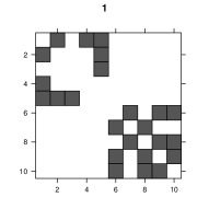
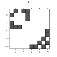
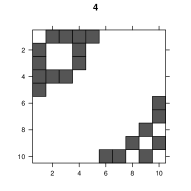
Figure 2: Shared sparsity patterns for four $10\times 10$ precision matrices. for elements ${\cal{G}}_{x,ii^{\prime}}$ in the upper $5\times 5$ block, matrices (1,2) and (3,4) have the same non-zero support, i.e. ${\cal{G}}_{x,ii^{\prime}}=\{(1,2),(3,4)\}$. On the other hand, when $i,i^{\prime}$ are in the lower block, ${\cal{G}}_{x,ii^{\prime}}=\{(1,3),(2,4)\}$

We assume an element-wise group sparsity pattern over $k$ for the precision matrices $\Omega_{x}^{k}$:

$${\cal{G}}_{x}=\{{\cal{G}}_{x}^{ii^{\prime}}:i\neq i^{\prime};i,i^{\prime}\in{\cal{I}}_{p}\},$$

where each ${\cal{G}}_{x}^{ii^{\prime}}$ is a partition of ${\cal{I}}_{K}$, and consists of non-overlapping index groups $g$ such that $g\subseteq{\cal{I}}_{K},\cup_{g\in{\cal{G}}_{x}^{ii^{\prime}}}g={\cal{I}}_{K}$. First introduced in Ma and Michailidis (2016), this formulation helps incorporate group structures that are common across some of the precision matrices being modeled. Figure 2 illustrates this through a small example. Subsequently, we use the Joint Structural Estimation Method (JSEM, Ma and Michailidis (2016)) to estimate $\Omega_{x}$, which first uses the group structure given by ${\cal{G}}_{x}$ in penalized nodewise regressions (Meinshausen and Bühlmann, 2006) to obtain neighborhood coefficients $\zeta_{i}=({\boldsymbol{\zeta}}_{i}^{1},\ldots,{\boldsymbol{\zeta}}_{i}^{K})$ of each variable $X_{i},i\in{\cal{I}}_{p}$, then fits a maximum likelihood model over the combined support sets to obtain sparse estimates of the precision matrices:

$$\widehat{\zeta}_{i} =\operatorname*{arg\,min}_{\zeta_{i}}\left\{\frac{1}{n}\sum_{k=1}^{K}\|{\mathbf{X}}_{i}^{k}-{\mathbf{X}}_{-i}^{k}{\boldsymbol{\zeta}}_{i}^{k}\|^{2}+\sum_{i^{\prime}\leq i}\sum_{g\in{\cal{G}}_{x}^{ii^{\prime}}}\eta_{n}\|{\boldsymbol{\zeta}}_{ii^{\prime}}^{[g]}\|\right\},$$

$$\widehat{E}_{x}^{k} =\{(i,i^{\prime}):1\leq i<i^{\prime}\leq p,\hat{\zeta}_{ii^{\prime}}^{k}\neq 0\text{ OR }\hat{\zeta}_{i^{\prime}i}^{k}\neq 0\},$$

$$\widehat{\Omega}_{x}^{k} =\operatorname*{arg\,min}_{\Omega_{x}^{k}\in{\mathbb{S}}_{+}(\hat{E}_{x}^{k})}\left\{\operatorname*{Tr}(\widehat{\mathbf{S}}_{x}^{k}\Omega_{x}^{k})-\log\det(\Omega_{x}^{k})\right\}.$$ (4)

where $\widehat{\mathbf{S}}_{x}^{k}:=({\mathbf{X}}^{k})^{T}{\mathbf{X}}^{k}/n$, $\eta_{n}$ is a tuning parameter, and ${\mathbb{S}}_{+}(\hat{E}_{x}^{k})$ is the set of positive-definite matrices that have non-zero supports restricted to $\hat{E}_{x}^{k}$.

For the precision matrices $\Omega_{y}^{k}$, we assume an element-wise sparsity pattern ${\cal{G}}_{y}$ defined in a similar manner as ${\cal{G}}_{x}$. The sparsity structure ${\cal{H}}$ for ${\cal{B}}$ is more general, each non-overlapping group $h\in{\cal{H}}$ being defined as:

$$h=\{({\cal{S}}_{p},{\cal{S}}_{q},{\cal{S}}_{K}):{\cal{S}}_{p}\subseteq{\cal{I}}_{p},{\cal{S}}_{q}\subseteq{\cal{I}}_{q},{\cal{S}}_{K}\subseteq{\cal{I}}_{K}\};\quad\bigcup_{h\in{\cal{H}}}h={\cal{I}}_{p}\times{\cal{I}}_{q}\times{\cal{I}}_{K}.$$

In other words, any arbitrary partition of ${\cal{I}}_{p}\times{\cal{I}}_{q}\times{\cal{I}}_{K}$ can be specified as the sparsity pattern of ${\cal{B}}$.

Denote the neighborhood coefficients of the $j^{\operatorname*{{}^{\text{th}}}}$ variable in the lower layer by ${\boldsymbol{\theta}}_{j}^{k}$, and $\Theta_{j}:=({\boldsymbol{\theta}}_{j}^{1},\ldots,{\boldsymbol{\theta}}_{j}^{K}),\Theta=\{\Theta_{j}\}$. We obtain sparse estimates of ${\cal{B}},\Theta$, and subsequently $\Omega_{y}$, by solving the following group-penalized least square minimization problem that has the tuning parameters $\gamma_{n}$ and $\lambda_{n}$ and then refitting:

$$\{\widehat{\cal{B}},\widehat{\Theta}\} =\operatorname*{arg\,min}_{{\cal{B}},\Theta}\left\{\frac{1}{n}\sum_{j=1}^{q}\sum_{k=1}^{K}\|{\mathbf{Y}}^{k}_{j}-({\mathbf{Y}}_{-j}^{k}-{\mathbf{X}}^{k}{\mathbf{B}}_{-j}^{k}){\boldsymbol{\theta}}_{j}^{k}-{\mathbf{X}}^{k}{\mathbf{B}}_{j}^{k}\|^{2}\right.$$

$$\left.+\sum_{j\neq j^{\prime}}\sum_{g\in{\cal{G}}_{y}^{jj^{\prime}}}\gamma_{n}\|{\boldsymbol{\theta}}_{jj^{\prime}}^{[g]}\|+\sum_{h\in{\cal{H}}}\lambda_{n}\|{\mathbf{B}}^{[h]}\|\right\},$$ (5)

$$\widehat{E}_{y}^{k} =\{(j,j^{\prime}):1\leq j<j^{\prime}\leq q,\hat{\theta}_{jj^{\prime}}^{k}\neq 0\text{ OR }\hat{\theta}_{j^{\prime}j}^{k}\neq 0\},$$

$$\widehat{\Omega}_{y}^{k} =\operatorname*{arg\,min}_{\Omega_{y}^{k}\in{\mathbb{S}}_{+}(\hat{E}_{y}^{k})}\left\{\operatorname*{Tr}(\widehat{\mathbf{S}}_{y}^{k}\Omega_{y}^{k})-\log\det(\Omega_{y}^{k})\right\}.$$ (6)

The outcome of a node in the lower layer is thus modeled using all other nodes in that layer using the neighborhood coefficients $\widehat{\mathbf{B}}_{j}^{k}$, and nodes in the immediate upper layer using the regression coefficients $\widehat{\boldsymbol{\theta}}_{j}^{k}$.

Remark 1

Common sparsity structures across the same layer are incorporated into the regression by the group penalties over the element-wise groups ${\boldsymbol{\theta}}_{jj^{\prime}}^{[g]}$, while sparsity pattern overlaps across the different regression matrices ${\mathbf{B}}^{k}$ are handled by the group penalties over ${\mathbf{B}}^{[h]}$, which denote the collection of elements in ${\cal{B}}$ that are in $h$. Other kinds of structural assumptions on ${\cal{B}}$ or $\Theta$ can be handled within the above structure by swapping out the group norms in favor of other appropriate norm-based penalties.

Remark 2

Group sparsity assumptions are not necessary for the JMMLE framework: rather, they help leverage additional information regarding interaction of features in and between the layers in many applications, as and when that information is available. In the vertical direction of the model, i.e. given a fixed $k$, a framework agnostic of any structural dependency assumptions amounts to element-wise groups in ${\mathbf{B}}^{k}$ and $\Omega_{y}^{k}$. In JMMLE, this occurs by construction for $\Theta$, and since ${\cal{H}}$ consists of all possible partitions of ${\cal{I}}_{p}\times{\cal{I}}_{q}\times{\cal{I}}_{K}$, it covers the case of element-wise groups as well. On the other hand, the absence of any horizontal (i.e. across $k$) dependency simply decomposes the problems (5) and (6) into $K$ independent sub-problems that can be solved separately either by setting $K=1$ in our framework or by using existing methods, such as Lin et al. (2016a). The proposed framework provides signficant more generality and aims at tight vertical and horizontal integration based on available prior information.

2.2.1 Alternating Block Algorithm

The objective function in (5) is bi-convex, i.e. convex in ${\cal{B}}$ for fixed $\Theta$, and vice-versa, but not jointly convex in $\{{\cal{B}},\Theta\}$. Consequently, we use an alternating iterative algorithm to solve for $\{{\cal{B}},\Theta\}$ that minimizes (5) by iteratively cycling between ${\cal{B}}$ and $\Theta$, i.e. holding one set of parameters fixed and solving for the other, then alternating until convergence.

Choice of initial values plays a crucial role in the performance of this algorithm as discussed in detail in Lin et al. (2016a). We choose the initial values $\{\widehat{\mathbf{B}}^{k(0)}\}$ by fitting separate lasso regression models for each $j$ and $k$:

$$\widehat{\mathbf{B}}_{j}^{k(0)}=\operatorname*{arg\,min}_{{\mathbf{B}}_{j}^{k}\in{\mathbb{R}}^{p}}\|{\mathbf{Y}}_{j}^{k}-{\mathbf{X}}^{k}{\mathbf{B}}_{j}^{k}\|^{2}+\lambda_{n}\|{\mathbf{B}}_{j}^{k}\|_{1};\quad j\in{\cal{I}}_{q},k\in{\cal{I}}_{K}.$$ (7)

We obtain initial estimates of $\Theta_{j},j\in{\cal{I}}_{q}$ by performing group-penalized nodewise regression on the residuals $\widehat{\mathbf{E}}^{k(0)}:={\mathbf{Y}}^{k}-{\mathbf{X}}^{k}\widehat{\mathbf{B}}_{j}^{k(0)}$:

$$\widehat{\Theta}_{j}^{(0)}=\operatorname*{arg\,min}_{\Theta_{j}}\frac{1}{n}\sum_{k=1}^{K}\|\widehat{\mathbf{E}}_{j}^{k(0)}-\widehat{\mathbf{E}}_{-j}^{k(0)}{\boldsymbol{\theta}}_{j}^{k}\|^{2}+\gamma_{n}\sum_{j\neq j^{\prime}}\sum_{g\in{\cal{G}}_{y}^{jj^{\prime}}}\|{\boldsymbol{\theta}}_{jj^{\prime}}^{[g]}\|.$$ (8)

The steps of our full estimation procedure, coined as the Joint Multiple Multi-Layer Estimation (JMMLE) method, are summarized in Algorithm 1.

Algorithm 1

(The JMMLE Algorithm)

1. Initialize $\widehat{\cal{B}}$ using (7).

2. Initialize $\widehat{\Theta}$ using (8).

3. Update $\widehat{\cal{B}}$ as:

$$\widehat{\cal{B}}^{(t+1)} =\operatorname*{arg\,min}_{\begin{subarray}{c}{\mathbf{B}}^{k}\in{\mathbb{M}}(p,q)\\ k\in{\cal{I}}_{K}\end{subarray}}\left\{\frac{1}{n}\sum_{j=1}^{q}\sum_{k=1}^{K}\|{\mathbf{Y}}^{k}_{j}-({\mathbf{Y}}_{-j}^{k}-{\mathbf{X}}^{k}{\mathbf{B}}_{-j}^{k})\widehat{\boldsymbol{\theta}}_{j}^{k(t)}-{\mathbf{X}}^{k}{\mathbf{B}}_{j}^{k}\|^{2}+\lambda_{n}\sum_{h\in{\cal{H}}}\|{\mathbf{B}}^{[h]}\|\right\}$$ (9)

4. Obtain $\widehat{\mathbf{E}}^{k(t+1)}:={\mathbf{Y}}^{k}-{\mathbf{X}}^{k}{\mathbf{B}}_{j}^{k(t)},k\in{\cal{I}}_{K}$. Update $\widehat{\Theta}$ as:

$$\widehat{\Theta}_{j}^{(t+1)}=\operatorname*{arg\,min}_{\Theta_{j}\in{\mathbb{M}}(q-1,K)}\left\{\frac{1}{n}\sum_{k=1}^{K}\|\widehat{\mathbf{E}}_{j}^{k(t+1)}-\widehat{\mathbf{E}}_{-j}^{k(t+1)}{\boldsymbol{\theta}}_{j}^{k}\|^{2}+\gamma_{n}\sum_{j\neq j^{\prime}}\sum_{g\in{\cal{G}}_{y}^{jj^{\prime}}}\|{\boldsymbol{\theta}}_{jj^{\prime}}^{[g]}\|\right\}$$ (10)

5. Continue till convergence.

6. Calculate $\widehat{\Omega}_{y}^{k},k\in{\cal{I}}_{K}$ using (6).

2.2.2 Tuning parameter selection

A number of methods have been proposed in the literature to select regularization tuning parameters in $\ell_{1}$-penalized problems. Some approaches rely on traditional criteria like cross-validation, Akaike Information Criterion (AIC) (Danaher et al., 2014) or the Bayesian Information Criterion (BIC) (Lin et al., 2016a; Ma and Michailidis, 2016). A number of studies have proposed their modifications for the case when feature dimensions increase with sample size (Foygel and Drton, 2010; Gao et al., 2012; Kim et al., 2012).

As a demonstration, to select the tuning parameter $\lambda_{n}$ we use the High-dimensional BIC (HBIC, Kim et al. (2012); Wang et al. (2013)), and for selecting $\gamma_{n}$ in the node-wise regression step in the JSEM model (2.2), employ BIC as in Ma and Michailidis (2016). Unlike BIC, the penalty term in HBIC scales with the parameter dimensions. As a result, the tuning parameter selected as the minimizer of HBIC asymptotically identifies the oracle estimator in ultra-high dimensional penalized problems (Fan and Tang, 2013; Wang et al., 2013). In our case, we train multiple JMMLE models using Algorithm 1 over a finite set of values $\lambda_{n}\in{\cal{D}}_{n}$, and calculate their HBIC:

$$\text{HBIC}(\lambda_{n};\Theta) =\frac{1}{n}\sum_{j=1}^{q}\sum_{k=1}^{K}\|{\mathbf{Y}}^{k}_{j}-({\mathbf{Y}}_{-j}^{k}-{\mathbf{X}}^{k}\widehat{\mathbf{B}}_{-j,\lambda_{n}}^{k}){\boldsymbol{\theta}}_{j}^{k}-{\mathbf{X}}^{k}\widehat{\mathbf{B}}_{j,\lambda_{n}}^{k}\|^{2}+$$

$$\log(\log n)\frac{\log(pq)}{n}\sum_{k=1}^{K}\left(\|{\mathbf{B}}^{k}\|_{0}+|\widehat{E}_{y,\gamma_{n}^{*}(\lambda_{n})}^{k}|\right).$$

Following this step, we select the optimal $\lambda_{n}$ as the empirical minimizer of HBIC over ${\cal{D}}_{n}$: $\lambda^{*}=\operatorname*{arg\,min}_{\lambda_{n}\in{\cal{D}}_{n}}\text{HBIC}(\lambda,\widehat{\Theta}_{\gamma_{n}^{*}(\lambda_{n})})$.

The step for updating $\Theta$ (i.e. (10) in Algorithm 1) in our JMMLE algorithm is analogous to the JSEM method Ma and Michailidis (2016), hence we use BIC to select the penalty parameter $\gamma_{n}$. In our setting the BIC for a given $\gamma_{n}$ and fixed ${\cal{B}}$ is given by:

$$\text{BIC}(\gamma_{n};{\cal{B}}) =\operatorname*{Tr}\left({\mathbf{S}}_{y}^{k}\widehat{\Omega}_{y,\gamma_{n}}^{k}\right)-\log\det\left(\widehat{\Omega}_{y,\gamma_{n}}^{k}\right)+\frac{\log n}{n}\sum_{k=1}^{K}|\widehat{E}_{y,\gamma_{n}}^{k}|$$

where $\gamma_{n}$ in subscript indicates the corresponding quantity is calculated taking $\gamma_{n}$ as the tuning parameter, and ${\mathbf{S}}_{y}^{k}:=({\mathbf{Y}}^{k}-{\mathbf{X}}^{k}{\mathbf{B}}^{k})^{T}({\mathbf{Y}}^{k}-{\mathbf{X}}^{k}{\mathbf{B}}^{k})/n$. Every time $\widehat{\Theta}$ is updated in the JMMLE algorithm, we choose the optimal $\gamma_{n}$ as the one with the smallest BIC over a fixed set of values ${\cal{C}}_{n}$. Thus for a fixed $\lambda_{n}\equiv\lambda$, our final choice of $\gamma_{n}$ will be $\gamma_{n}^{*}(\lambda)=\operatorname*{arg\,min}_{\gamma_{n}\in{\cal{C}}_{n}}\text{BIC}(\gamma_{n};\widehat{\cal{B}}_{\lambda_{n}})$.

2.3 Properties of JMMLE estimators

We now provide theoretical results ensuring the convergence of our alternating algorithm, as well as the consistency of estimators obtained from the algorithm. We present statements of theorems in the main body of the paper, while detailed proofs and auxiliary results are delegated to the Appendix.

We introduce some additional notation and define technical conditions that help establish the results that follow. Denote the true values of the parameters by $\Omega_{x0}=\{\Omega_{x0}^{k}\},\Omega_{y0}=\{\Omega_{y0}^{k}\},\Theta_{0}=\{\Theta_{0j}\},{\cal{B}}_{0}=\{{\mathbf{B}}_{0}^{k}\}$. Sparsity levels of individual true parameters are indicated by $s_{j}:=|\operatorname*{supp}(\Theta_{0j})|,b_{k}:=|\operatorname*{supp}({\mathbf{B}}^{k}_{0})|$. Also define $S:=\sum_{j=1}^{q}s_{j},B:=\sum_{k=1}^{K}b_{k},s:=\max_{j\in{\cal{I}}_{q}}s_{j}$, and ${\cal{X}}:=\{{\mathbf{X}}^{k}\}_{k=1}^{K},{\cal{E}}:=\{{\mathbf{E}}^{k}\}_{k=1}^{K}$.

Definition 3 (Bounded eigenvalues)

A positive definite matrix $\Sigma\in{\mathbb{M}}(b,b)$ is said to have bounded eigenvalues with constants $(c_{0},d_{0})$ if

$$0<1/c_{0}\leq\Lambda_{\min}(\Sigma)\leq\Lambda_{\max}(\Sigma)\leq 1/d_{0}<\infty$$

Definition 4 (Diagonal dominance)

A matrix ${\mathbf{M}}\in{\mathbb{M}}(b,b)$ is said to be strictly diagonally dominant if for all $a\in{\cal{I}}_{b}$,

$$|({\mathbf{M}})_{aa}|>\sum_{a^{\prime}\neq a}|({\mathbf{M}})_{aa^{\prime}}|$$

Denote $\Delta_{0}({\mathbf{M}})=\min_{a}\{|({\mathbf{M}})_{aa}|-\sum_{a^{\prime}\neq a}|({\mathbf{M}})_{aa^{\prime}}|\}$.

Our first result establishes the convergence of Algorithm 1 for fixed realizations of $({\cal{X}},{\cal{E}})$.

Theorem 5

Suppose for any fixed $({\cal{X}},{\cal{E}})$, estimates in each iterate of Algorithm 1 are uniformly bounded by some quantity dependent on only $p,q$ and $n$:

$$\left\|(\widehat{\cal{B}}^{(t)},\widehat{\Theta}_{y}^{(t)})-({\cal{B}}_{0},\Theta_{y0})\right\|_{F}\leq R(p,q,n);\quad t\geq 1$$ (11)

Then, any limit point $({\cal{B}}^{\infty},\Theta_{y}^{\infty})$ of the algorithm is a stationary point of the objective function, i.e. a point where partial derivatives along all coordinates are non-negative.

As established in Theorems 6 and 7, at sub-iterations of Algorithm 1 (specifically steps 3 and 4) a $O(\sqrt{\log(pq)}/n)$ bound on $\widehat{\cal{B}}^{(t)}$ leads to $\widehat{\Theta}^{(t+1)}$ being consistent for $\Theta_{0}$, and a $O(\sqrt{\log q}/n)$ bound on $\widehat{\Theta}^{(t)}$ leads to $\widehat{\cal{B}}^{(t+1)}$ being consistent for ${\cal{B}}_{0}$: both with probability approaching 1 as $p,q,n\rightarrow\infty$. Thus, while the constant $R(p,q,n)$ in Theorem 5 above does not need to obey any explicit bounds for Algorithm 1 to have a limit point, having a tighter $O(\sqrt{\log(pq)}/n)$ bound ensures that the limit point lies close to the population parameters with high enough probability.

The next steps establish that for random realizations of ${\cal{X}}$ and ${\cal{E}}$, (a) successive iterates lie in this non-expanding ball around the true parameters, and (b) the procedures in (7) and (8) ensure starting values that lie inside the same ball, both with probability approaching 1 as $(p,q,n)\rightarrow\infty$. To do so, we break down the main problem into two sub-problems. Take as ${\boldsymbol{\beta}}=(\operatorname*{vec}({\mathbf{B}}^{1})^{T},\ldots,\operatorname*{vec}({\mathbf{B}}^{K})^{T})^{T}$: any subscript or superscript on ${\mathbf{B}}$ being passed on to ${\boldsymbol{\beta}}$. Denote by $\widehat{\Theta}$ and $\widehat{\boldsymbol{\beta}}$ the generic estimators given by

$$\widehat{\Theta}_{j} =\operatorname*{arg\,min}_{\Theta_{j}\in{\mathbb{M}}(q-1,K)}\left\{\frac{1}{n}\sum_{k=1}^{K}\|\widehat{\mathbf{E}}^{k}_{j}-\widehat{\mathbf{E}}^{k}_{-j}{\boldsymbol{\theta}}_{j}^{k}\|^{2}+\gamma_{n}\sum_{j\neq j^{\prime}}\sum_{g\in{\cal{G}}_{y}^{jj^{\prime}}}\|{\boldsymbol{\theta}}_{jj^{\prime}}^{[g]}\|\right\};\quad j\in{\cal{I}}_{q},$$ (12)

$$\widehat{\boldsymbol{\beta}} =\operatorname*{arg\,min}_{{\boldsymbol{\beta}}\in{\mathbb{R}}^{pqK}}\left\{-2{\boldsymbol{\beta}}^{T}\widehat{\boldsymbol{\gamma}}+{\boldsymbol{\beta}}^{T}\widehat{\boldsymbol{\Gamma}}{\boldsymbol{\beta}}+\lambda_{n}\sum_{h\in{\cal{H}}}\|{\boldsymbol{\beta}}^{[h]}\|\right\},$$ (13)

where

$$\widehat{\boldsymbol{\Gamma}}=\begin{bmatrix}(\widehat{\mathbf{T}}^{1})^{2}\otimes\frac{({\mathbf{X}}^{1})^{T}{\mathbf{X}}^{1}}{n}&&\\ &\ddots&\\ &&(\widehat{\mathbf{T}}^{K})^{2}\otimes\frac{({\mathbf{X}}^{K})^{T}{\mathbf{X}}^{K}}{n}\end{bmatrix};\quad\widehat{\boldsymbol{\gamma}}=\begin{bmatrix}(\widehat{\mathbf{T}}^{1})^{2}\otimes\frac{({\mathbf{X}}^{1})^{T}}{n}\\ \vdots\\ (\widehat{\mathbf{T}}^{K})^{2}\otimes\frac{({\mathbf{X}}^{K})^{T}}{n}\end{bmatrix}\begin{bmatrix}\operatorname*{vec}({\mathbf{Y}}^{1})\\ \vdots\\ \operatorname*{vec}({\mathbf{Y}}^{K})\end{bmatrix},$$

with

$$\hat{T}_{jj^{\prime}}^{k}=\begin{cases}1&\text{ if }j=j^{\prime}\\ -\hat{\theta}_{jj^{\prime}}^{k}&\text{ if }j\neq j^{\prime}\end{cases}.$$ (14)

Using matrix algebra it is easy to see that solving for ${\cal{B}}$ in (5) given a fixed $\widehat{\Theta}$ is equivalent to solving (13).

Next, we assume the following conditions:

(E1) The matrices $\Omega_{y0}^{k},k\in{\cal{I}}_{K}$ are diagonally dominant,

(E2) The matrices $\Sigma_{y0}^{k},k\in{\cal{I}}_{K}$ have bounded eigenvalues with constants $(c_{y},d_{y})$ that are common across $k$.

Now, we are in a position to establish the estimation consistency for (12), as well as the consistency of the final estimates $\widehat{\Omega}_{y}^{k}$ using their support sets.

Theorem 6

Consider random $({\cal{X}},{\cal{E}})$, any deterministic $\widetilde{\cal{B}}$ that satisfy the following bound

$$\|\widetilde{\mathbf{B}}^{k}-{\mathbf{B}}_{0}^{k}\|_{1}\leq C_{\beta}\sqrt{\frac{\log(pq)}{n}},$$

where $C_{\beta}$ depends only on ${\cal{B}}_{0}$. Then, for sample size $n\succsim\log(pq)$ there exist constants $c_{1},c_{3},c_{4}>0,c_{2},c_{5}>1,\tau_{1}>2$ such that with probability at least

$$1-K(1/p^{\tau_{1}-2}-c_{1}\exp[-(c_{2}^{2}-1)\log(pq)]-2\exp(-c_{3}n)-c_{4}\exp[-(c_{5}^{2}-1)\log(pq)]),$$

the following bounds hold:

(I) Denote $|g_{\max}|=\max_{g\in{\cal{G}}_{y}}|g|$. Then for the choice of tuning parameter

$$\gamma_{n}\geq 4\sqrt{|g_{\max}|}{\mathbb{Q}}_{0}\sqrt{\frac{\log(pq)}{n}},$$

where ${\mathbb{Q}}_{0}$ depends on the model parameters only, we have

$$\|\widehat{\Theta}_{j}-\Theta_{0,j}\|_{F} \leq 12\sqrt{s_{j}}\gamma_{n}/\psi,$$ (15)

$$\sum_{j\neq j^{\prime},g\in{\cal{G}}_{y}^{jj^{\prime}}}\|\hat{\boldsymbol{\theta}}_{jj^{\prime}}^{[g]}-{\boldsymbol{\theta}}_{0,jj^{\prime}}^{[g]}\| \leq 48s_{j}\gamma_{n}/\psi.$$ (16)

with $\psi=\min_{k}\Lambda_{\min}(\Sigma_{x0}^{k})/2$.

(II) For the choice of tuning parameter $\gamma_{n}=4\sqrt{|g_{\max}|}{\mathbb{Q}}_{0}\sqrt{\log(pq)/n}$,

$$\frac{1}{K}\sum_{k=1}^{K}\|\widehat{\Omega}_{y}^{k}-\Omega_{y0}^{k}\|_{F}\leq O\left({\mathbb{Q}}_{0}\sqrt{\frac{|g_{\max}|S}{K}}\sqrt{\frac{\log(pq)}{n}}\right).$$ (17)

Condition (E2) ensures that the lower layer covariance matrices are well-conditioned, so that the precision matrices $\{\Omega_{y}^{k}\}$ exist. The diagonal dominance condition (E1) is a sufficient condition for the convergence bounds of Theorem 6 to hold. Specifically, the upper bounds of the finite-sample error rates of estimates $\widehat{\Theta}$ and $\widehat{\Omega}_{y}$ are controlled by the ratios of off-diagonal to diagonal elements, i.e. $\omega_{y,jj}^{k}/\sum_{j^{\prime}\neq j}|\omega_{y,jj^{\prime}}^{k}|$ through the multiplier ${\mathbb{Q}}_{0}$. A number of $\ell_{1}$-penalized problems make Restricted Eigenvalue (RE)-type assumptions (Bickel et al., 2009; Loh and Wainwright, 2012; Lin et al., 2016a) on the (upper layer) design matrices. Following Basu and Michailidis (2015); Lin et al. (2016a) (see Lemma B.1 and Proposition 1 in respective papers), we utilize the diagonal dominance condition to ensure RE conditions for some key model quantities.

To prove an equivalent result for the solution of (13), we need the following conditions on the true parameter versions $({\mathbf{T}}_{0}^{k})^{2}$, defined from $\Theta_{0}$ similarly as (14).

(E3) The matrices $({\mathbf{T}}_{0}^{k})^{2},k\in{\cal{I}}_{K}$ are diagonally dominant,

(E4) The matrices $\Sigma_{x0}^{k},k\in{\cal{I}}_{K}$ have bounded eigenvalues with common constants $(c_{x},d_{x})$.

Given these, we next establish the required consistency results.

Theorem 7

Assume random $({\cal{X}},{\cal{E}})$, and fixed $\widetilde{\Theta}$ so that for $j\in{\cal{I}}_{q}$,

$$\|\widetilde{\Theta}_{j}-\Theta_{0,j}\|_{F}\leq C_{\Theta}\sqrt{\frac{\log q}{n}}$$

for some $C_{\Theta}$ dependent on $\Theta_{0}$ only. Then, given the choice of tuning parameter

$$\lambda_{n}\geq 4\sqrt{|h_{\max}|}{\mathbb{R}}_{0}\sqrt{\frac{\log(pq)}{n}},$$

where ${\mathbb{R}}_{0}$ depends on the population parameters only, with probability at least

$$1-K(c_{1}\exp[-(c_{2}^{2}-1)\log(pq)]-2\exp(-c_{3}n))$$

the following bounds hold:

$$\|\widehat{\boldsymbol{\beta}}-{\boldsymbol{\beta}}_{0}\|_{1} \leq 48\sqrt{|h_{\max}|}B\lambda_{n}/\psi_{*},$$ (18)

$$\|\widehat{\boldsymbol{\beta}}-{\boldsymbol{\beta}}_{0}\| \leq 12\sqrt{B}\lambda_{n}/\psi_{*},$$ (19)

$$\sum_{h\in{\cal{H}}}\|{\boldsymbol{\beta}}^{[h]}-{\boldsymbol{\beta}}_{0}^{[h]}\| \leq 48B\lambda_{n}/\psi_{*},$$ (20)

$$(\widehat{\boldsymbol{\beta}}-{\boldsymbol{\beta}}_{0})^{T}\widehat{\boldsymbol{\Gamma}}(\widehat{\boldsymbol{\beta}}-{\boldsymbol{\beta}}_{0}) \leq 72B\lambda_{n}^{2}/\psi_{*},$$ (21)

where $|h_{\max}|=\max_{h\in{\cal{H}}}|h|$, $d_{k}$ is the maximum degree $({\mathbf{T}}_{0}^{k})^{2}$, and

$$\psi_{*}=\frac{1}{2}\min_{k}\left[\Lambda_{\min}(\Sigma_{x0}^{k})\left(\Delta_{0}(({\mathbf{T}}_{0}^{k})^{2})-d_{k}C_{\Theta}\sqrt{\frac{\log(pq)}{n}}\right)\right].$$

Remark 8

In an effort to keep the JMMLE framework as general as possible, we do not impose any explicit sparsity conditions on the fixed quantities $\widetilde{\cal{B}}$ and $\widetilde{\Theta}$ used to estimate the other parameter inside an iteration of Algorithm 1. Since $C_{\beta}$ (or $C_{\Theta}$) depends only on the population parameter ${\cal{B}}_{0}$ (or $\Theta_{0}$), when that parameter is actually sparse their corresponding sparsity values can be a part of $C_{\beta}$ (or $C_{\Theta}$). When we do obtain the actual estimates ((15)–(17) in Theorem 6 and (18)–(21) in Theorem 7), their finite-sample error bounds scale with the corresponding sparsity parameters $\{s_{j}\}$ and $B$ at rates that are standard in the literature (Basu and Michailidis, 2015; Loh and Wainwright, 2012; Ravikumar et al., 2011).

Following the choice of tuning parameters in Theorems 6 and 7, $S=o(n/\log(pq))$ and $B=o(n/\log(pq))$ are sufficient conditions on the sparsity of corresponding parameters for the JMMLE estimators to be consistent. As the last step to establish estimation consistency for the limit points of Algorithm 1, we now ensure that the starting values are satisfactory as previously discussed.

Theorem 9

Consider the starting values as derived in (7) and (8). For sample size $n\succsim\log(pq)$, and the choice of the tuning parameter

$$\lambda_{n}\geq 4c_{2}\max_{k\in{\cal{I}}_{K}}\left\{[\Lambda_{\max}(\Sigma_{x0}^{k})\Lambda_{\max}(\Sigma_{y0}^{k})]^{1/2}\right\}\sqrt{\frac{\log(pq)}{n}},$$

we have $\|\widehat{\boldsymbol{\beta}}^{(0)}-{\boldsymbol{\beta}}_{0}\|_{1}\leq 64B\lambda_{n}/\psi^{*}$ with probability at least $1-c_{1}\exp(-(c_{2}^{2}-1)\log(pq))-2\exp(c_{3}n)$. Also, for $\gamma_{n}\geq 4\sqrt{|g_{\max}|}{\mathbb{Q}}_{0}\sqrt{\log(pq)/n}$ we have

$$\|\widehat{\Theta}_{j}^{(0)}-\Theta_{0,j}\|_{F} \leq 12\sqrt{s_{j}}\gamma_{n}/\psi,$$

$$\sum_{j\neq j^{\prime},g\in{\cal{G}}_{y}^{jj^{\prime}}}\|\hat{\boldsymbol{\theta}}_{jj^{\prime}}^{[g](0)}-{\boldsymbol{\theta}}_{0,jj^{\prime}}^{[g]}\| \leq 48s_{j}\gamma_{n}/\psi,$$

with probability at least

$$1-K(1/p^{\tau_{1}-2}-c_{1}\exp[-(c_{2}^{2}-1)\log(pq)]-2\exp(-c_{3}n)-c_{4}\exp[-(c_{5}^{2}-1)\log(pq)]).$$

Putting all the pieces together, the required consistency result given our choice of starting values follows in a straightforward manner.

Corollary 10

Assume conditions (E1)-(E4), and starting values $\{{\cal{B}}^{(0)},\Theta^{(0)}\}$ obtained using (7) and (8), respectively. Then, for random realizations of ${\cal{X}},{\cal{E}}$,

(I) For the choice of $\lambda_{n}$

$$\lambda_{n}\geq 4\max\left[c_{2}\max_{k\in{\cal{I}}_{K}}\left\{[\Lambda_{\max}(\Sigma_{x0}^{k})\Lambda_{\max}(\Sigma_{y0}^{k})]^{1/2}\right\},\sqrt{|h_{\max}|}{\mathbb{R}}_{0}\right]\sqrt{\frac{\log(pq)}{n}},$$

we have

$$\|\widehat{\boldsymbol{\beta}}-{\boldsymbol{\beta}}_{0}\|_{1}\leq\max\left\{48\sqrt{|h_{\max}|},64\right\}\frac{B\lambda_{n}}{\psi_{*}}$$

with probability at least $1-18c_{1}\exp[-(c_{2}^{2}-1)\log(pq)]-4\exp(-c_{3}n)$.

(II) For the choice of $\gamma_{n}$

$$\gamma_{n}\geq 4\sqrt{|g_{\max}|}{\mathbb{Q}}_{0}\sqrt{\frac{\log(pq)}{n}},$$

(15) and (16) hold, while for $\gamma_{n}=4\sqrt{|g_{\max}|}{\mathbb{Q}}_{0}\sqrt{\log(pq)/n}$, (17) holds, both with probability at least

$$1-K(2/p^{\tau_{1}-2}-2c_{1}\exp[-(c_{2}^{2}-1)\log(pq)]-4\exp(-c_{3}n)-2c_{4}\exp[-(c_{5}^{2}-1)\log(pq)]).$$

Remark 11

To save computation time for high data dimensions, an initial screening step, e.g. the debiased lasso procedure of Javanmard and Montanari (2014), can be used to first restrict the support set of ${\mathbf{B}}_{j}^{k}$ before obtaining the initial estimates using (7). The consistency properties of resulting initial and final estimates follow along the lines of the special case $K=1$ discussed in Lin et al. (2016a), in conjunction with Theorem 9 and Corollary 10, respectively. We leave the details to the reader.

Remark 12

While the proof of the above results follow roughly similar roadmaps as the case with $K=1$ and simple $\ell_{1}$-penalization (Lin et al., 2016a) and the joint structural estimation of Ma and Michailidis (2016) and utilize Gaussian concentration inequalities, generalization to $K>1$ and an optional grouping structure in ${\cal{B}}$ add significant additional technical complexity to the proofs. More importantly, we work in presence of minimal assumptions, steering clear of conditions used in previous works, like Incoherence (Lin et al., 2016a) and Uniform Irrepresentability (Ma and Michailidis, 2016) that are hard to verify in practice.

3 Hypothesis testing in multilayer models

In this section, we lay out a framework for hypothesis testing in our proposed joint multi-layer structure. Present literature in high-dimensional hypothesis testing either focuses on testing for similarities in the within-layer connections of single-layer networks (Cai and Liu, 2016; Liu, 2017), or coefficients of single response penalized regression (van de Geer et al., 2014; Zhang and Zhang, 2014; Mitra and Zhang, 2016). However, to our knowledge no method is available in the literature to perform testing for between-layer connections in a two-layer (or multi-layer) setup.

Denote the $i\operatorname*{{}^{\text{th}}}$ row of the coefficient matrix ${\mathbf{B}}^{k}$ by ${\bf{b}}_{i}^{k}$, for $i\in{\cal{I}}_{p}$. In this section we are generally interested in obtaining asymptotic sampling distributions of $\widehat{\bf{b}}_{i}^{k}$, and subsequently formulating testing procedures to detect similarities or differences across $k$ in the full vector ${\bf{b}}_{i}^{k}$ or its elements. There are two main challenges in doing the above: firstly the need to mitigate the bias of the group-penalized JMMLE estimators, and secondly the dependency among response nodes translating into the need for controlling false discovery rate while simultaneously testing for several element-wise hypotheses concerning the true values $b_{0ij}^{k},j\in{\cal{I}}_{q}$. To this end, in Section 3.1 we first propose a debiased estimator for ${\bf{b}}_{i}^{k}$ that makes use of already computed (using JSEM) node-wise regression coefficients in the upper layer, and establish asymptotic properties of scaled version of them. Section 3.2 is devoted to pairwise testing, where we assume $K=2$, and propose asymptotic global tests for detecting differential effects of a variable in the upper layer, i.e. testing for the null hypothesis $H_{0}^{i}:{\bf{b}}_{0i}^{1}={\bf{b}}_{0i}^{2}$, as well as pairwise simultaneous tests across $j\in{\cal{I}}_{q}$ for detecting the element-wise differences $b_{0ij}^{1}-b_{0ij}^{2}$.

3.1 Debiased estimators and asymptotic normality

Zhang and Zhang (2014) proposed a debiasing procedure for lasso estimates and subsequently calculate confidence intervals for individual coefficients $\beta_{j}$ in high-dimensional linear regression: ${\bf{y}}={\mathbf{X}}{\boldsymbol{\beta}}+{\boldsymbol{\epsilon}},{\bf{y}}\in{\mathbb{R}}^{n},{\mathbf{X}}\in{\mathbb{M}}(n,p)$ and $\epsilon_{r}\sim N(0,\sigma^{2}),r\in{\cal{I}}_{n}$ for some $\sigma>0$. Given an initial lasso estimate $\widehat{\boldsymbol{\beta}}^{\text{(init)}}\in{\mathbb{R}}^{p}$ their debiased estimator was defined as:

$$\hat{\beta}_{j}^{(\text{deb})}=\hat{\beta}_{j}^{(\text{init})}+\frac{{\bf{z}}_{j}^{T}({\bf{y}}-{\mathbf{X}}\hat{\boldsymbol{\beta}}^{(\text{init})})}{{\bf{z}}^{T}{\bf{x}}_{j}},$$

where ${\bf{z}}_{j}$ is the vector of residuals from the $\ell_{1}$-penalized regression of ${\bf{x}}_{j}$ on ${\mathbf{X}}_{-j}$. With centering around the true parameter value, say $\beta_{j}^{0}$, and proper scaling this has an asymptotic normal distribution:

$$\frac{\hat{\beta}_{j}^{(\text{deb})}-\beta_{j}^{0}}{\|{\bf{z}}_{j}\|/|{\bf{z}}_{j}^{T}{\bf{x}}_{j}|}\sim N(0,\sigma^{2}).$$

Essentially, they obtain the debiasing factor for the $j^{\operatorname*{{}^{\text{th}}}}$ coefficient by taking residuals from the regularized regression and scale them using the projection of ${\bf{x}}_{j}$ onto a space approximately orthogonal to it. Mitra and Zhang (2016) later generalized this idea to group lasso estimates. Further, van de Geer et al. (2014) and Javanmard and Montanari (2014) performed debiasing on the entire coefficient vectors.

We start off by defining debiased estimates for individual rows of the coefficient matrices ${\mathbf{B}}^{k}$ in our two-layer model:

$$\widehat{\bf{c}}_{i}^{k}=\widehat{\bf{b}}_{i}^{k}+\frac{1}{nt_{i}^{k}}\left({\mathbf{X}}_{i}^{k}-{\mathbf{X}}_{-i}^{k}\widehat{\boldsymbol{\zeta}}_{i}^{k}\right)^{T}({\mathbf{Y}}^{k}-{\mathbf{X}}^{k}\widehat{\mathbf{B}}^{k});\quad i\in{\cal{I}}_{p},k\in{\cal{I}}_{K},$$ (22)

where $\widehat{\bf{b}}_{i}^{k}$ denotes the $i\operatorname*{{}^{\text{th}}}$ row of $\widehat{\mathbf{B}}^{k}$, and $t_{i}^{k}=({\mathbf{X}}_{i}^{k}-{\mathbf{X}}_{-i}^{k}\widehat{\boldsymbol{\zeta}}_{i}^{k})^{T}{\mathbf{X}}_{i}^{k}/n$, and $\widehat{\boldsymbol{\zeta}}_{i}^{k},\widehat{\mathbf{B}}^{k}$ are generic estimators of the neighborhood coefficient matrices in the upper layer and within-layer coefficient matrices, respectively. By structure this is similar to the proposal of Zhang and Zhang (2014). However, as seen shortly, minimal conditions need to be imposed on the parameter estimates used in (22) for the asymptotic results based on a scaled version of the debiased estimator to go thorugh, and they continue to hold for arbitrary sparsity patterns over $k$ in all of the parameters.

Present methods of debiasing coefficients from regularized regression require specific assumptions on the regularization structure of the main regression, as well as on how to calculate the debiasing factor. While Zhang and Zhang (2014), Javanmard and Montanari (2014) and van de Geer et al. (2014) work on coefficients from lasso regressions, Mitra and Zhang (2016) debias the coefficients of pre-specified groups in the coefficient vector from a group lasso. Current proposals for obtaining the debiasing factor available in the literature include node-wise lasso (Zhang and Zhang, 2014) and a variance minimization scheme with $\ell_{\infty}$-constraints (Javanmard and Montanari, 2014). In comparison, we only assume the following generic constraints on the parameter estimates used in our procedure.

(T1) For the upper layer neighborhood coefficients, the following holds for all $k\in{\cal{I}}_{K}$:

$$\|\widehat{\boldsymbol{\zeta}}^{k}-{\boldsymbol{\zeta}}_{0}^{k}\|_{1}\leq D_{\zeta}=O\left(\sqrt{\frac{\log p}{n}}\right),$$

where $D_{\zeta}$ depends only on the true values, i.e. $\{\zeta^{k}_{0}\}$.

(T2) The lower layer precision matrix estimates satisfy for all $k\in{\cal{I}}_{K}$

$$\|\widehat{\Omega}_{y}^{k}-\Omega_{y0}^{k}\|_{\infty}\leq D_{\Omega}=O\left(\sqrt{\frac{\log(pq)}{n}}\right),$$

where $D_{\Omega}$ depends only on $\Omega_{y0}$.

(T3) For the regression coefficient matrices, the following holds for all $k\in{\cal{I}}_{K}$:

$$\|\widehat{\mathbf{B}}^{k}-{\mathbf{B}}^{k}_{0}\|_{1}\leq D_{\beta}=O\left(\sqrt{\frac{\log(pq)}{n}}\right),$$

where $D_{\beta}$ depends on ${\cal{B}}_{0}$ only.

The above finite-sample error rates are common in high-dimensional problems, and can pertain to sparse (Ma and Michailidis, 2016; Lin et al., 2016a; Loh and Wainwright, 2012; Basu and Michailidis, 2015) or non-sparse estimators (Rohde and Tsybakov, 2011; Basu et al., 2019). Based on the estimators plugged in, additional conditions may be involved in the estimation step. For example, JMMLE estimators satisfy these bounds under conditions (E1)-(E4) following the results in Section 2.3.

Given these conditions, the following result provides the asymptotic joint distribution of a scaled version of the debiased coefficients. A similar result for fixed design in the context of single-response linear regression can be found in Stucky and van de Geer (2018). However, the authors use the nuclear norm as the loss function while obtaining the debiasing factors and employ the resulting Karush-Kuhn-Tucker (KKT) conditions to derive their results, whereas we leverage bounds on generic parameter estimates combined with the sub-Gaussianity of our random design matrices.

Theorem 13

Define $\widehat{s}_{i}^{k}=\sqrt{\|{\mathbf{X}}_{i}^{k}-{\mathbf{X}}_{-i}^{k}\widehat{\boldsymbol{\zeta}}_{i}^{k}\|^{2}/n}$, and $m_{i}^{k}=\sqrt{n}t_{i}^{k}/\widehat{s}_{i}^{k}$. Consider parameter estimates that satisfy conditions (T1)-(T3). Define the following:

$$\widehat{\Omega}_{y} =\operatorname*{diag}(\widehat{\Omega}_{y}^{1},\ldots,\widehat{\Omega}_{y}^{K}),$$

$${\mathbf{M}}_{i} =\operatorname*{diag}(m_{i}^{1},\ldots,m_{i}^{K}),$$

$$\widehat{\mathbf{C}}_{i} =\operatorname*{vec}(\widehat{\bf{c}}_{i}^{1},\ldots,\widehat{\bf{c}}_{i}^{K})^{T},$$

$${\mathbf{D}}_{i} =\operatorname*{vec}({\bf{b}}_{0i}^{1},\ldots,{\bf{b}}_{0i}^{K})^{T}.$$

Also assume that conditions (E2), (E4) hold, and the matrices $\Omega_{x0}^{k},k\in{\cal{I}}_{K}$ are diagonally dominant. Then, for sample size satisfying $\log p=o(n^{1/2}),\log q=o(n^{1/2})$ we have

$$\widehat{\Omega}_{y}^{1/2}{\mathbf{M}}_{i}(\widehat{\mathbf{C}}_{i}-{\mathbf{D}}_{i})\sim{\cal{N}}_{Kq}({\bf 0},{\mathbf{I}})+{\mathbf{R}}_{n},$$ (23)

where $\|{\mathbf{R}}_{n}\|_{\infty}=o_{P}(1)$.

3.2 Test formulation

We now simply plug in estimators from the JMMLE algorithm in Theorem 13. Doing so is fairly straightforward. Condition (T1) is ensured by the JSEM penalized neighborhood estimators in (2.2) (immediate from Proposition A.1 in Ma and Michailidis (2016)). On the other hand, bounds on total sparsity of the true coefficient matrices: $B=o(\sqrt{n}/\log(pq))$, and lower layer precision matrices: $S=o(n/\log(pq)$, in conjunction with Corollary 10, ensure conditions (T2) and (T3), respectively -all with probability approaching 1 as $(n,p,q)\rightarrow\infty$.

An asymptotic joint distribution of debiased versions of the JMMLE regression estimates can then be obtained immediately.

Corollary 14

Consider the estimates $\widehat{\cal{B}}$ and $\widehat{\Omega}_{y}$ obtained from Algorithm 1, and upper layer neighborhood coefficients from solving the node-wise regression in (2.2). Suppose that $\log(pq)/\sqrt{n}\rightarrow 0$, and the sparsity conditions $B=o(\sqrt{n}/\log(pq)),S=o(n/\log(pq))$ are satisfied. Then, with the same notations as in Theorem 13 we have

$$\widehat{\Omega}_{y}^{1/2}{\mathbf{M}}_{i}(\widehat{\mathbf{C}}_{i}-{\mathbf{D}}_{i})\sim{\cal{N}}_{Kq}({\bf 0},{\mathbf{I}})+{\mathbf{R}}_{1n}$$ (24)

where $\|{\mathbf{R}}_{1n}\|_{\infty}=o_{P}(1)$.

We are now ready to formulate asymptotic global and simultaneous testing procedures based on Corollary 14. In this paper, we restrict our attention to testing for pairwise differences only. Specifically, we set $K=2$, and are interested in testing whether there are overall and elementwise differences between individual rows of the true coefficient matrices, i.e. ${\bf{b}}_{0i}^{1}$ and ${\bf{b}}_{0i}^{2}$.

When ${\bf{b}}_{0i}^{1}={\bf{b}}_{0i}^{2}$, it is immediate from Corollary 14 that a scaled version of the vector of estimated differences $\widehat{\bf{c}}_{i}^{1}-\widehat{\bf{c}}_{i}^{2}$ follows a $q$-variate multivariate normal distribution. Consequently, we formulate a global test for detecting differential overall downstream effect of the $i^{\operatorname*{{}^{\text{th}}}}$ covariate in the upper layer.

Algorithm 2

(Global test for $H_{0}^{i}:{\bf{b}}_{0i}^{1}={\bf{b}}_{0i}^{2}$ at level $\alpha,0<\alpha<1$)

1. Obtain the debiased estimators $\widehat{\bf{c}}_{i}^{1},\widehat{\bf{c}}_{i}^{2}$ using (22).

2. Calculate the test statistic

$$D_{i}=(\widehat{\bf{c}}_{i}^{1}-\widehat{\bf{c}}_{i}^{2})^{T}\left(\frac{\widehat{\Sigma}_{y}^{1}}{(m_{i}^{1})^{2}}+\frac{\widehat{\Sigma}_{y}^{2}}{(m_{i}^{2})^{2}}\right)^{-1}(\widehat{\bf{c}}_{i}^{1}-\widehat{\bf{c}}_{i}^{2})$$

where $\widehat{\Sigma}_{y}^{k}=(\widehat{\Omega}_{y}^{k})^{-1},k=1,2$.

3. Reject $H_{0}^{i}$ if $D_{i}\geq\chi^{2}_{q,1-\alpha}$.

Besides controlling the type-I error at a specified level, the above testing procedure maintains rate optimal power.

Theorem 15

Consider the global test given in Algorithm 2, performed using parameter estimates satisfying conditions (T1)-(T3). Define ${\boldsymbol{\delta}}:={\bf{b}}_{0i}^{1}-{\bf{b}}_{0i}^{2}$. Further, assume that either of the following sufficient conditions are satisfied.

• The following bound holds: $D_{\Omega}\leq\Delta_{0}(\Omega_{y0}^{k}),k\in{\cal{I}}_{K}$;

• For every $j\in{\cal{I}}_{q},k\in{\cal{I}}_{K}$, we have $\sum_{j^{\prime}=1}^{q}|\sigma_{y0,jj^{\prime}}^{k}|^{q}\leq c_{0}(p)$ for some $q\in[0,1)$ and positive-valued function $c_{0}(\cdot)$.

Denote $\sigma_{x0,i,-i}^{k}=Var(X_{i}^{k}-{\mathbb{X}}_{-i}^{k}{\boldsymbol{\zeta}}_{0,i}^{k})$. Then, the power of the global test is given by

$$K_{q}\left(\chi^{2}_{q,1-\alpha}+n{\boldsymbol{\delta}}^{T}\left(\frac{\Sigma_{y0}^{1}}{\sigma_{x0,i,-i}^{1}}+\frac{\Sigma_{y0}^{2}}{\sigma_{x0,i,-i}^{2}}\right)^{-1}{\boldsymbol{\delta}}\right)+o(1)$$

where $K_{q}$ is the cumulative distribution function of the $\chi^{2}_{q}$ distribution. Consequently, for $\|{\boldsymbol{\delta}}\|>O(n^{-1/2})$, $P(H_{0}^{i}\text{ is rejected })\rightarrow 1$ as $(n,p,q)\rightarrow\infty$.

The conditions (I) or (II) above are needed to derive upper bounds for $\|\widehat{\Sigma}_{y}^{k}-\Sigma_{y0}^{k}\|_{\infty}$ using those for $\|\widehat{\Omega}_{y}^{k}-\Omega_{y0}^{k}\|_{\infty}$. While (I) imposes a potentially more stringent bound on the estimation error of $\Omega_{y}$, (II) restricts the power calculations to a uniformity class of covariance matrices (Bickel and Levina, 2008; Cai et al., 2012b).

Remark 16

While the formulation of the testing procedure broadly gives parallel results as Zhang and Zhang (2014) and Mitra and Zhang (2016), it does so without assuming any specific penalty function or (group) sparsity conditions (such as strong group sparsity in Mitra and Zhang (2016)). Instead, we only require the standard finite-sample bounds (T1)-(T3), satisfied by existing sparse and non-sparse estimators in a high-dimensional setting.

3.3 Control of False Discovery Rate

Given that the null hypothesis is rejected, we consider the multiple testing problem of simultaneously testing for all entrywise differences, i.e. testing

$$H_{0}^{ij}:b_{0ij}^{1}=b_{0ij}^{2}\quad\text{vs.}\quad H_{1}^{ij}:b_{0ij}^{1}\neq b_{0ij}^{2}$$

for all $j\in{\cal{I}}_{q}$. Here we use the test statistic

$$d_{ij} =\frac{\widehat{c}_{ij}^{1}-\widehat{c}_{ij}^{2}}{\sqrt{\hat{\sigma}_{jj}^{1}/(m_{i}^{1})^{2}+\hat{\sigma}_{jj}^{2}/(m_{i}^{2})^{2}}},$$ (25)

with $\hat{\sigma}_{jj}^{k}$ being the $j^{\operatorname*{{}^{\text{th}}}}$ diagonal element of $\widehat{\Sigma}_{y}^{k},k=1,2$.

For the purpose of simultaneous testing, we consider tests with a common rejection threshold $\tau$, i.e. for $j\in{\cal{I}}_{q}$, $H_{0}^{ij}$ is rejected if $|d_{ij}|>\tau$. We denote ${\cal{H}}_{0}^{i}=\{j:b_{0,ij}^{1}=b_{0,ij}^{2}\}$ and define the False Discovery Proportion (FDP) and False Discovery Rate (FDR) for these tests as follows:

$$FDP(\tau)=\frac{\sum_{j\in{\cal{H}}_{0}^{i}}{\mathbb{I}}(|d_{ij}|\geq\tau)}{\max\left\{\sum_{j\in{\cal{I}}_{q}}{\mathbb{I}}(|d_{ij}|\geq\tau),1\right\}};\quad FDR(\tau)={\mathbb{E}}[FDP(\tau)].$$

For a pre-specified level $\alpha$, we choose a threshold that ensures both FDP and FDR $\leq\alpha$ using the Benjamini-Hochberg (BH) procedure. The procedure for FDR control is now given by Algorithm 3.

Algorithm 3

(Simultaneous tests for $H_{0}^{ij}:b_{0ij}^{1}=b_{0ij}^{2}$ at level $\alpha,0<\alpha<1$)

1. Calculate the pairwise test statistics $d_{ij}$ using (3) for $j\in{\cal{I}}_{q}$.

2. Obtain the threshold

$$\hat{\tau}=\inf\left\{\tau\in{\mathbb{R}}:1-\Phi(\tau)\leq\frac{\alpha}{2q}\max\left(\sum_{j\in{\cal{I}}_{q}}{\mathbb{I}}(|d_{ij}|\geq\tau),1\right)\right\}.$$

3. For $j\in{\cal{I}}_{q}$, reject $H_{0}^{ij}$ if $|d_{ij}|\geq\hat{\tau}$.

To ensure that this procedure maintains FDR and FDP asymptotically at a pre-specified level $\alpha\in(0,1)$, we need some dependence conditions on true correlation matrices in the lower layer. Following Liu and Shao (2014), we consider the following two types of dependencies:

(D1) Define $r_{jj^{\prime}}^{k}=\sigma_{y0,jj^{\prime}}^{k}/\sqrt{\sigma_{y0,jj}^{k}\sigma_{y0,j^{\prime}j^{\prime}}^{k}}$ for $j,j^{\prime}\in{\cal{I}}_{q},k=1,2$. Suppose there exists $0<r<1$ such that $\max_{1\leq j<j^{\prime}\leq q}|r_{jj^{\prime}}^{k}|\leq r$, and for every $j\in{\cal{I}}_{q}$,

$$\sum_{j^{\prime}=1}^{q}{\mathbb{I}}\left\{|r_{jj^{\prime}}^{k}|\geq\frac{1}{(\log q)^{2+\theta}}\right\}\leq O(q^{\rho}),$$

for some $\theta>0$ and $0<\rho<(1-r)/(1+r)$.

(D1*) Suppose there exists $0<r<1$ such that $\max_{1\leq j<j^{\prime}\leq q}|r_{jj^{\prime}}^{k}|\leq r$, and for every $j\in{\cal{I}}_{q}$,

$$\sum_{j^{\prime}=1}^{q}{\mathbb{I}}\left\{|r_{jj^{\prime}}^{k}|>0\right\}\leq O(q^{\rho}),$$

for some $0<\rho<(1-r)/(1+r)$.

Originally proposed by Liu and Shao (2014), the above dependency conditions are meant to control the amount of correlation amongst the test statistics. Condition (D1) allows each variable to be highly correlated with at most $O(q^{\rho})$ other variables and weakly correlated with others, while (D1*) limits the number of variables to have any correlation with it to $O(q^{\rho})$. Note that (D1*) is a stronger condition, and can be seen as the limiting condition of (D1) as $q\rightarrow\infty$.

Theorem 17

Suppose $\mu_{j}=b_{0,ij}^{1}-b_{0,ij}^{2},\sigma_{j}^{2}=\sigma_{y0,jj}^{1}/\sigma_{x0,i,-i}^{1}+\sigma_{y0,jj}^{2}/\sigma_{x0,i,-i}^{2}$. Assume the following holds as $(n,q)\rightarrow\infty$,

$$\left|\left\{j\in{\cal{I}}_{q}:|\mu_{j}/\sigma_{j}|\geq 4\sqrt{\log q/n}\right\}\right|\rightarrow\infty.$$ (26)

Next, consider conditions (D1) and (D1*). If (D1) is satisfied, then the following holds when $\log q=O(n^{\xi}),0<\xi<3/23$:

$$\frac{FDP(\hat{\tau})}{(|{\cal{H}}_{0}^{i}|/q)\alpha}\stackrel{{\scriptstyle P}}{{\rightarrow}}1;\quad\lim_{n,q\rightarrow\infty}\frac{FDR(\hat{\tau})}{(|{\cal{H}}_{0}^{i}|/q)\alpha}=1.$$ (27)

Further, if (D1*) is satisfied, then (27) holds for $\log q=o(n^{1/3})$.

The condition (26) is essential for FDR control in a diverging parameter space (Liu and Shao, 2014; Liu, 2017).

Remark 18

Based on the FDR control procedure in Algorithm 3, we can perform within-row thresholding in the matrices $\widehat{\mathbf{B}}^{k}$ to tackle group misspecification.

$$\hat{\tau}_{i}^{k}:=\inf\left\{\tau\in{\mathbb{R}}:1-\Phi(\tau)\leq\frac{\alpha}{2q}\max\left(\sum_{j\in{\cal{I}}_{q}}{\mathbb{I}}(|\sqrt{\hat{\omega}_{jj}^{k}}m_{i}^{k}\hat{c}_{ij}^{k}|\geq\tau),1\right)\right\},$$

$$\hat{b}_{ij}^{k,\text{thr}}=\hat{b}_{ij}^{k}{\mathbb{I}}\left(|\sqrt{\hat{\omega}_{jj}^{k}}m_{i}^{k}\hat{c}_{ij}^{k}|\geq\hat{\tau}_{i}^{k}\right).$$ (28)

Even without group misspecification, this helps identify directed edges between layers that have high nonzero values. Similar post-estimation thresholdings have been proposed in the context of multitask regression (Obozinski et al., 2011; Majumdar and Chatterjee, 2018) and neighborhood selection (Ma and Michailidis, 2016). However, our procedure is the first one to provide explicit guarantees on the amount of false discoveries while doing so.

Remark 19

Following (26), a sufficient condition on the sparsity of ${\cal{B}}_{0}$ for FDR to be asymptotically controlled at some specified level is $B=o(n^{\zeta}/\log q)$ if (D1) is satisfied, and $B=o(n^{1/3}/\log q)$ if (D1*) is satisfied. In comparison, our results for the global testing procedure require $B=o(\sqrt{n}/\log(pq))$, and point estimation requires $B=o(n/\log(pq))$. In finite samples settings, the stricter sparsity requirements translate to higher sample sizes being needed (given the same $(p,q)$) for our testing procedures to have satisfactory performances compared to estimation only (See Sections 4.1 and 4.2).

In recent work, Javanmard and Montanari (2018) showed that the $o(\sqrt{n}/\log p)$ bound on the sparsity of the true coefficient vector required to construct confidence intervals from debiased lasso coefficient estimates (van de Geer et al., 2014; Zhang and Zhang, 2014; Javanmard and Montanari, 2014) can be weakened to $o(n/(\log p)^{2})$ when the random design precision matrix is known, or is unknown but satisfies certain sparsity assumptions. Similar relaxations may be possible in our case. For example, the machinery in Liu (2017), which performs simultaneous testing in multiple (single layer) GGMs using slightly modified FDR thresholds, can be useful in obtaining (27) for $\log q=o(n^{1/2})$ under (D1), (D1*) or other suitable dependency assumptions.

3.4 Effect of tuning parameter selection

A topic not adequately addressed in the high-dimensional hypothesis testing literature concerns the effect of the regularization tuning parameter selection methods (HBIC for $\lambda_{n}$ and BIC for $\gamma_{n}$ in our case) on the size, power and confidence intervals obtained. Ideally, tuning parameter selection method(s) in the estimation step should ensure that the estimated quantities from the model with optimal tuning parameter choices can be plugged into the debiasing procedure to obtain quantities that obey the correct asymptotic properties and are used in the tests that follow (e.g. Algorithms 2 and 3).

In our case, the broad-based assumptions (T1)-(T3) allow plugging in estimators with finite-sample error rates that are satisfied by a host of high-dimensional methods, as previously discussed. Given that the tuning parameters $\lambda_{n}$ and $\gamma_{n}$ are selected to be above thresholds that scale with feature and sample dimensions, JMMLE estimators adhere to these error rates with high probability (Corollary 10), ensuring the correctness of our testing procedures. To empirically make it likely that the correct tuning parameters get selected, in our numerical examples (on synthetic and real data) that follow, we obtain JMMLE estimates over ranges of $\lambda_{n}$ and $\gamma_{n}$ that scale with the error rates of estimators. Additional technicalities will be involved for a more rigorous analysis, possibly using technical material from approaches such as Foygel and Drton (2010); Wang et al. (2013). We defer this topic to future work.

4 Numerical experiments

We evaluate the performance of our proposed JMMLE algorithm and the hypothesis testing framework in a two-layer simulation setup (Sections 4.1 and 4.2, respectively), and also introduce some computational techniques that significantly accelerate calculations for high data dimensions (Section 4.3).

4.1 Simulation 1: estimation

As a first step towards obtaining a two-layer structure with horizontal (across $k$) integration and inter-layer directed edges, we generate the precision matrices $\{\Omega_{x0}^{k}\}$ and $\{\Omega_{y0}^{k}\}$ using a dependency structure across $k$ that was first used in the simulation study of Ma and Michailidis (2016). We set $K=5$, and set different shared sparsity patterns across $k$ inside the lower $p/2\times p/2$ block of the upper layer precision matrices, and outside the block. In our notation, this gives the following elementwise group structure:

$${\cal{G}}_{x,ii^{\prime}}=\begin{cases}\{(1,2),(3,4),5\}&\text{ if }i\leq p/2\text{ or }j\leq p/2,\\ \{(1,3,5),(2,4)\}&\text{ otherwise}.\end{cases}$$

Figure 3: Shared sparsity patterns across $k$ for the precision matrices $\{\Omega_{x0}^{k}\}$ and $\{\Omega_{y0}^{k}\}$

The schematic in Figure 3 illustrates this structure. We set an off-diagonal element inside each of these common blocks (i.e. $A,B,C$ and $\alpha,\beta$ in the figure) to be non-zero with probability $\pi_{x}\in\{5/p,30/p\}$, then generate the values of all non-zero elements independently from the uniform distribution in the interval $[-1,0.5]\cup[0.5,1]$. The precision matrices $\Omega_{x0}^{k}$ are generated by putting together the corresponding common blocks, their positive definiteness ensured by setting all diagonal elements to be $1+|\Lambda_{\min}(\Omega_{x0}^{k})|$. Then, we get elements in the covariance matrix as

$$\sigma_{x0,ii^{\prime}}^{k}=(\bar{\Omega}_{x0}^{k})_{ii^{\prime}}/\sqrt{(\bar{\Omega}_{x0}^{k})_{ii}(\bar{\Omega}_{x0}^{k})_{i^{\prime}i^{\prime}}},\text{ where }\bar{\Omega}_{x0}^{k}=(\Omega_{x0}^{k})^{-1},$$

and generate rows of ${\mathbf{X}}^{k}$ independently from ${\cal{N}}(0,\Sigma_{x0}^{k})$. We obtain $\Sigma_{y0}^{k}$ and then ${\mathbf{E}}^{k}$ using the same setup but with the number of variables being $q$ and setting off-diagonal elements non-zero with probability $\pi_{y}\in\{5/q,30/q\}$. To obtain the matrices ${\mathbf{B}}_{0}^{k}$, for a fixed $(i,j),i\in{\cal{I}}_{p},j\in{\cal{I}}_{q}$, we set $b_{0,ij}^{k}$ non-zero across all $k$ with probability $\pi\in\{5/p,30/p\}$, generate the non-zero groups independently from $\text{Unif}\{[-1,0.5]\cup[0.5,1]\}$, and set ${\mathbf{Y}}^{k}={\mathbf{X}}^{k}{\mathbf{B}}_{0}^{k}+{\mathbf{E}}^{k},k\in{\cal{I}}_{K}$. Finally, we generate 150 such independent two-layer datasets for each of the following model settings:

• Set $\pi_{x}=\pi=5/p,\pi_{y}=5/q$, and

  $$(p,q,n)\in\{(60,30,100),(30,60,100),(200,200,150),(300,300,150)\};$$

• Set $\pi_{x}=\pi=30/p,\pi_{y}=30/q$, and $(p,q,n)\in\{(200,200,100),(200,200,200)\}$.

We use the following scaled arrays of tuning parameters to train Algorithm 1-

$$\gamma_{n}\in\left\{0.3,0.4,...,1\right\}\sqrt{\frac{\log q}{n}};\quad\lambda_{n}\in\left\{0.4,0.6,...,1.8\right\}\sqrt{\frac{\log p}{n}},$$

using a one-step version of the algorithm (Section 4.3) to save computation time.

We use the following performance metrics to evaluate our estimates $\widehat{\cal{B}}=\{\widehat{\mathbf{B}}^{k}\}$:

• True positive Rate-

  $$\text{TPR}(\widehat{\mathbf{B}}_{k})=\frac{|\operatorname*{supp}(\hat{\mathbf{B}}^{k})\cap\operatorname*{supp}({\mathbf{B}}_{0}^{k})|}{|\operatorname*{supp}({\mathbf{B}}_{0}^{k})|};\quad\text{TPR}(\widehat{\cal{B}})=\frac{1}{K}\sum_{k=1}^{K}\text{TP}(\widehat{\mathbf{B}}_{k}).$$

• True negative Rate-

  $$\text{TNR}(\widehat{\mathbf{B}}_{k})=\frac{|{\operatorname*{supp}}^{c}(\hat{\mathbf{B}}^{k})\cap{\operatorname*{supp}}^{c}({\mathbf{B}}_{0}^{k})|}{|\operatorname*{supp}^{c}({\mathbf{B}}_{0}^{k})|};\quad\text{TNR}(\widehat{\cal{B}})=\frac{1}{K}\sum_{k=1}^{K}\text{TNR}(\widehat{\mathbf{B}}_{k}).$$

• Matthews Correlation Coefficient-

  $$\text{TP}(\widehat{\mathbf{B}}_{k})=|\operatorname*{supp}(\hat{\mathbf{B}}^{k})\cap\operatorname*{supp}({\mathbf{B}}_{0}^{k})|;\quad\text{TN}(\widehat{\mathbf{B}}_{k})=|{\operatorname*{supp}}^{c}(\hat{\mathbf{B}}^{k})\cap{\operatorname*{supp}}^{c}({\mathbf{B}}_{0}^{k})|,$$

  $$\text{FP}(\widehat{\mathbf{B}}_{k})=|{\operatorname*{supp}}^{c}({\mathbf{B}}^{k}_{0})|-\text{TN}(\widehat{\mathbf{B}}_{k});\quad\text{FN}(\widehat{\mathbf{B}}_{k})=|{\operatorname*{supp}}({\mathbf{B}}^{k}_{0})|-\text{TP}(\widehat{\mathbf{B}}_{k}),$$

  $$\text{MCC}(\widehat{\mathbf{B}}_{k})=$$

  $$\frac{\text{TP}(\widehat{\mathbf{B}}_{k})\text{TN}(\widehat{\mathbf{B}}_{k})-\text{FP}(\widehat{\mathbf{B}}_{k})\text{FN}(\widehat{\mathbf{B}}_{k})}{\sqrt{(\text{TP}(\widehat{\mathbf{B}}_{k})+\text{FP}(\widehat{\mathbf{B}}_{k}))(\text{TP}(\widehat{\mathbf{B}}_{k})+\text{FN}(\widehat{\mathbf{B}}_{k}))(\text{TN}(\widehat{\mathbf{B}}_{k})+\text{FP}(\widehat{\mathbf{B}}_{k}))(\text{TN}(\widehat{\mathbf{B}}_{k})+\text{FN}(\widehat{\mathbf{B}}_{k}))}},$$

  $$\text{MCC}(\widehat{\cal{B}})=\frac{1}{K}\sum_{k=1}^{K}\text{MCC}(\widehat{\mathbf{B}}_{k}).$$

• Relative error in Frobenius norm-

  $$\text{RF}(\widehat{\cal{B}})=\frac{1}{K}\sum_{k=1}^{K}\frac{\|\hat{\mathbf{B}}^{k}-{\mathbf{B}}_{0}^{k}\|_{F}}{\|{\mathbf{B}}_{0}^{k}\|_{F}}.$$

We use the same metrics to evaluate the precision matrix estimates $\widehat{\Omega}_{y}^{k}$ as well, with TPR and TNR calculations confined to off-diagonal entries.

$(\pi_{x},\pi_{y})$	$(p,q,n)$	Method	TPR	TNR	MCC	RF
$(5/p,5/q)$	(60,30,100)	JMMLE	0.97(0.02)	0.99(0.003)	0.96(0.014)	0.24(0.033)
		Separate	0.96(0.018)	0.99(0.004)	0.93(0.014)	0.22(0.029)
	(30,60,100)	JMMLE	0.97(0.013)	0.99(0.002)	0.96(0.008)	0.27(0.024)
		Separate	0.99(0.009)	0.99(0.003)	0.93(0.017)	0.18(0.021)
	(200,200,150)	JMMLE	0.98(0.011)	1.0(0)	0.99(0.005)	0.16(0.025)
		Separate	0.99(0.001)	0.99 (0.001)	0.88(0.009)	0.18(0.007)
	(300,300,150)	JMMLE	1.0(0.001)	1.0(0)	0.99(0.001)	0.14 (0.015)
		Separate	1.0(0.001)	0.99(0.001)	0.84(0.01)	0.21(0.007)
$(30/p,30/q)$	(200,200,100)	JMMLE	0.97(0.017)	1.0(0)	0.98(0.008)	0.21(0.032)
		Separate	0.32(0.01)	0.99(0.001)	0.49(0.009)	0.85(0.06)
	(200,200,200)	JMMLE	0.99(0.006)	1.0(0)	0.99(0.007)	0.13(0.016)
		Separate	0.97(0.004)	0.98(0.001)	0.93(0.002)	0.19(0.07)

Table 1: Table of outputs for estimation of regression matrices, giving empirical mean and standard deviation (in brackets) of each evaluation metric over 150 replications.

$(\pi_{x},\pi_{y})$	$(p,q,n)$	Method	TPR	TNR	MCC	RF
$(5/p,5/q)$	(60,30,100)	JMMLE	0.76(0.018)	0.90(0.006)	0.61(0.024)	0.32(0.008)
		Separate	0.77(0.031)	0.92(0.007)	0.56(0.03)	0.51(0.017)
		JSEM	0.24(0.013)	0.8(0.003)	0.05(0.015)	1.03(0.002)
	(30,60,100)	JMMLE	0.7(0.018)	0.94(0.002)	0.55(0.018)	0.3(0.005)
		Separate	0.76(0.041)	0.89(0.015)	0.59(0.039)	0.49(0.014)
		JSEM	0.13(0.005)	0.9(0.001)	0.03(0.007)	1.04(0.001)
	(200,200,150)	JMMLE	0.68(0.017)	0.98(0)	0.48(0.013)	0.26(0.002)
		Separate	0.78(0.019)	0.97(0.001)	0.55(0.012)	0.6(0.007)
		JSEM	0.05(0.002)	0.97(0)	0.02(0.002)	1.01(0)
	(300,300,150)	JMMLE	0.71(0.014)	0.98(0)	0.44(0.008)	0.25(0.002)
		Separate	0.71(0.017)	0.98(0.001)	0.51(0.011)	0.59(0.005)
		JSEM	0.04(0.002)	0.98(0)	0.02(0.002)	1.01(0)
$(30/p,30/q)$	(200,200,100)	JMMLE	0.77(0.016)	0.98(0)	0.46(0.013)	0.31(0.003)
		Separate	0.57(0.027)	0.44(0.007)	0.04(0.008)	0.84(0.002)
		JSEM	0.05(0.002)	0.97(0)	0.01(0.002)	1.01(0)
	(200,200,200)	JMMLE	0.76(0.018)	0.98(0)	0.55(0.015)	0.27(0.004)
		Separate	0.73(0.023)	0.94(0.003)	0.39(0.017)	0.62(0.011)
		JSEM	0.05(0.002)	0.97(0)	0.03(0.003)	1.01(0)

Table 2: Table of outputs for estimation of lower layer precision matrices over 150 replications.

Tables 1 and 2 summarize the results. For estimation of ${\cal{B}}$, we compare our results to the method in Lin et al. (2016a) that estimates parameters in each of the $K$ two-layer structure separately, while for estimation of $\Omega_{y}$, we compare them with the results in Lin et al. (2016a) and using the single-layer JSEM (Ma and Michailidis, 2016) that estimates $\Omega_{y}$ assuming structured sparsity patterns and centered matrices ${\mathbf{Y}}^{k}$, but not the data in the upper layer, i.e. ${\cal{X}}$.

Our joint method has higher average MCC across all data settings than the separate method for the estimation of ${\cal{B}}$, although TPR and TNR values are similar, except for $p=200,q=200,n=100$ where JMMLE has a much higher average TPR. For estimation of $\Omega_{y}$, incorporating information from the upper layer vastly improves performance, as demonstrated by the differences in performance between JMMLE and JSEM. For the 4 data settings with lower sparsity $(\pi_{x}=\pi=5/p,\pi_{y}=5/q)$, JMMLE produces sparser estimates compared to the separate method while estimating $\Omega_{y}$- as is evident from the lower TPR and MCC values. However, the RF values indicate that the quality of JMMLE estimates is significantly better. This in fact is a common pattern across the estimation of both ${\cal{B}}$ and $\Omega_{y}$: JMMLE gives more accurate estimates across the methods, with lower average RF values across all data settings. Finally, for the estimation of $\Omega_{y}$, JMMLE does better in both of the higher sparsity settings $(\pi_{x}=\pi=30/p,\pi_{y}=30/q)$ across all metrics.

$(\pi_{x},\pi_{y})$	$(p,q,n)$	TPR$(\widehat{\cal{B}})$	TNR$(\widehat{\cal{B}})$	MCC$(\widehat{\cal{B}})$	RF$(\widehat{\cal{B}})$
$(5/p,5/q)$	(60,30,100)	0.98 (0.01)	0.99 (0.002)	0.89 (0.017)	0.29 (0.014)
	(30,60,100)	0.94 (0.022)	0.99 (0.003)	0.93 (0.016)	0.31 (0.028)
	(200,200,150)	0.99 (0.002)	0.99 (0)	0.98 (0.004)	0.17 (0.007)
	(300,300,150)	0.99 (0.001)	1 (0)	0.99 (0.002)	0.15 (0.006)
$(30/p,30/q)$	(200,200,100)	0.99 (0.006)	1 (0)	0.98 (0.005)	0.2 (0.014)
	(200,200,200)	0.99 (0.009)	1 (0)	0.98 (0.005)	0.15 (0.017)
$(\pi_{x},\pi_{y})$	$(p,q,n)$	TPR$(\widehat{\Omega}_{y})$	TNR$(\widehat{\Omega}_{y})$	MCC$(\widehat{\Omega}_{y})$	RF$(\widehat{\Omega}_{y})$
$(5/p,5/q)$	(60,30,100)	0.71 (0.024)	0.90 (0.005)	0.64 (0.024)	0.34 (0.008)
	(30,60,100)	0.7 (0.019)	0.94 (0.002)	0.59 (0.014)	0.3 (0.004)
	(200,200,150)	0.62 (0.012)	0.98 (0)	0.43 (0.009)	0.27 (0.003)
	(300,300,150)	0.69 (0.013)	0.98 (0)	0.39 (0.008)	0.26 (0.02)
$(30/p,30/q)$	(200,200,100)	0.78 (0.024)	0.98 (0)	0.43 (0.012)	0.31 0.003)
	(200,200,200)	0.69 (0.026)	0.98 (0.001)	0.5 (0.02)	0.29 (0.004)

Table 3: Table of outputs for joint estimation in presence of group misspecification

$(\pi_{x},\pi_{y})$	$(p,q,n)$	FDR
$(5/p,5/q)$	(60,30,100)	0.19 (0.077)
	(30,60,100)	0.08 (0.064)
	(200,200,150)	0.04 (0.016)
	(300,300,150)	0.02 (0.007)
$(30/p,30/q)$	(200,200,100)	0.03 (0.019)
	(200,200,200)	0.03 (0.016)

Table 4: Table of outputs giving empirical FDR for estimating ${\cal{B}}$ using JMMLE in presence of group misspecification

4.1.1 Effect of heterogeneity

We repeat the above setups to check the performance of JMMLE in presence of within-group misspecification. For this task, we first set individual elements inside a non-zero group to be zero with probability 0.2 while generating the data, then pass the JMMLE estimates $\widehat{\mathbf{B}}^{k}$ through the FDR controlling thresholds as given in (28). The results are summarized in Tables 3 and 4. Across the simulation settings, values of all metrics are very close to the correctly specified counterparts in Table 1. Thus, the thresholding step proves largely effective. Also, in all cases the empirical FDR for estimating entries in ${\cal{B}}$ is below 0.2. The performance is slightly worse than the correctly specified cases when estimating $\Omega_{y}$. This is expected, as the estimates $\widehat{\Omega}_{y}$ are obtained from neighborhood coefficients that are calculated based on the pre-thresholding coefficient estimates.

$(\pi_{x},\pi_{y})$	$(p,q,n)$	Method	Global test		Simultaneous test
			Power	Size	Power	FDR
$(5/p,5/q)$	(60,30,100)	JMMLE	0.98 (0.016)	0.07 (0.011)	0.94 (0.023)	0.24 (0.027)
		Separate	0.99 (0.007)	0.12 (0.02)	0.91 (0.025)	0.34(0.038)
		SepLasso	0.99 (0.007)	0.11 (0.02)	0.91 (0.025)	0.33(0.038)
	(60,30,200)	JMMLE	0.99 (0.014)	0.07 (0.014)	0.97 (0.013)	0.22 (0.032)
		Separate	0.99 (0.005)	0.08 (0.014)	0.94 (0.019)	0.26(0.031)
		SepLasso	0.99 (0.004)	0.08 (0.014)	0.94 (0.019)	0.26(0.033)
	(30,60,100)	JMMLE	0.98 (0.024)	0.07 (0.014)	0.92 (0.027)	0.24 (0.035)
		Separate	1 (0)	0.07 (0.015)	0.86 (0.036)	0.25(0.039)
		SepLasso	1 (0)	0.08 (0.014)	0.85 (0.036)	0.25(0.039)
	(30,60,200)	JMMLE	0.99 (0.019)	0.08 (0.016)	0.96 (0.023)	0.24 (0.038)
		Separate	1 (0)	0.06 (0.013)	0.9 (0.038)	0.21(0.035)
		SepLasso	1 (0)	0.06 (0.012)	0.91 (0.038)	0.21(0.034)
	(200,200,150)	JMMLE	0.99 (0.006)	0.06 (0.003)	0.84 (0.011)	0.22 (0.007)
		Separate	1 (0)	0.2 (0.008)	0.93 (0.006)	0.46(0.009)
		SepLasso	1 (0)	0.2 (0.008)	0.93 (0.006)	0.46(0.009)
	(300,300,150)	JMMLE	0.99 (0.004)	0.07 (0.009)	0.54 (0.031)	0.34 (0.016)
		Separate	1 (0)	0.27 (0.01)	0.79 (0.007)	0.58(0.008)
		SepLasso	1 (0)	0.27 (0.01)	0.79 (0.007)	0.58(0.008)
	(300,300,300)	JMMLE	0.99 (0.003)	0.03 (0.002)	0.99 (0.003)	0.12 (0.006)
		Separate	1 (0)	0.16 (0.005)	0.99 (0.004)	0.4 (0.007)
		SepLasso	1 (0)	0.16 (0.005)	0.99 (0.004)	0.4 (0.007)
$(30/p,30/q)$	(200,200,100)	JMMLE	0.99 (0.005)	0.112 (0.003)	0.41 (0.008)	0.52 (0.007)
		Separate	1 (0)	0.47 (0.008)	0.75 (0.007)	0.71(0.004)
		SepLasso	1 (0)	0.47 (0.008)	0.75 (0.007)	0.71(0.004)
	(200,200,200)	JMMLE	0.99 (0.004)	0.09 (0.004)	0.96 (0.006)	0.27 (0.008)
		Separate	1 (0)	0.42 (0.011)	0.98 (0.005)	0.63(0.006)
		SepLasso	1 (0)	0.42 (0.011)	0.98 (0.005)	0.63(0.006)
	(200,200,300)	JMMLE	0.99 (0.002)	0.06 (0.003)	0.99 (0.004)	0.19 (0.008)
		Separate	1 (0)	0.27 (0.01)	0.99 (0.004)	0.52 (0.009)
		SepLasso	1 (0)	0.27 (0.01)	0.99 (0.004)	0.52 (0.009)

Table 5: Table of outputs for global and simultaneous hypothesis testing.

4.2 Simulation 2: testing

We slightly change the data generating model to evaluate our proposed global testing and FDR control procedure. We set $K=2$, then generate the ${\mathbf{B}}_{0}^{1}$ by first randomly assigning each of its element to be non-zero with probability $\pi$, then drawing values of those elements from $\text{Unif}\{[-1,-0.5]\cup[0.5,1]\}$ independently. After this we generate a matrix of differences ${\mathbf{D}}$, where $({\mathbf{D}})_{ij},i\in{\cal{I}}_{p},j\in{\cal{I}}_{q}$ takes values –1, 1, 0 with probabilities 0.1, 0.1 and 0.8, respectively. Finally we set ${\mathbf{B}}_{0}^{2}={\mathbf{B}}_{0}^{1}+{\mathbf{D}}$. We set identical sparsity structures for the pairs of precision matrices $\{\Omega_{x0}^{1},\Omega_{x0}^{2}\}$ and $\{\Omega_{y0}^{1},\Omega_{y0}^{2}\}$. We use 150 replications of the above setup to calculate empirical power of global tests, as well as empirical power and FDR of simultaneous tests. To get the empirical sizes of global tests we use estimators obtained from applying JMMLE on a separate set of data generated setting all elements of ${\mathbf{D}}$ to 0. The type-I error of global tests is controlled at level 0.05, while FDR is set at 0.2 obtained by calculating the respective thresholds.

Table 5 reports the empirical mean and standard deviations (in brackets) of all relevant quantities computed from debiased coefficients obtained from JMMLE, separate estimation, as well as from applying the original debiasing technique of Zhang and Zhang (2014) on $qK$ separate lasso estimates of row-level coefficient vectors, i.e. $\hat{\bf{b}}_{i}^{k}$. We report outputs for all combinations of data dimensions and sparsity used in Section 4.1, and also for increased sample sizes in each setting until a satisfactory FDR is reached. As expected from the theoretical analysis, higher sample sizes than those used in Section 4.1 result in increased power for both global and simultaneous tests, and decreased size and FDR for all but one ($p=30,q=60$) of the settings. While separate estimation has slightly higher power in global testing, our joint method gives better results everywhere else. The empirical size of the JMMLE-based global tests remain slightly higher than the nominal level across the settings considered. This is in all likelihood a consequence of the higher sample size requirements in testing than estimation, as nominal sizes for JMMLE estimates tend to go down when $p,q$ are kept constant and $n$ is increased (for example, check setting 6 vs. setting 7 ($p=300,,q=300,n=150,300)$, and setting 8 vs. 9 vs. 10 ($p=200,,q=200,n=100,200,300)$. This pattern is similar to empirical results in past proposals of high-dimensional testing methodology (Wang et al., 2015; Wu et al., 2020). However, the size estimates of JMMLE are much closer to the nominal level across data settings compared to either separate estimation or separate lasso, owing the fact that only JMMLE is able to leverage information across the different multilayer networks.

4.3 Computation

Next, we discuss some observations and strategies that speed up the JMMLE algorithm and reduce computation time significantly, especially for higher number of features in either layer.

Block update and refit ${\mathbf{B}}^{k}$ in each iteration.

Similar to the case of $K=1$ (Lin et al., 2016a), we use block coordinate descent within each ${\mathbf{B}}^{k}$. This means instead of the full update step (9) we perform the following steps in each iteration to speed up convergence:

$$\left\{\widehat{\mathbf{B}}^{k(t+1)}_{j}\right\}_{k=1}^{K}=\operatorname*{arg\,min}_{\begin{subarray}{c}{\bf{b}}_{j}^{k}\in{\mathbb{R}}^{p}\\ k\in{\cal{I}}_{K}\end{subarray}}\left\{\frac{1}{n}\sum_{j=1}^{q}\sum_{k=1}^{K}\|{\mathbf{Y}}^{k}_{j}+{\bf{r}}_{j}^{k(t)}-{\mathbf{X}}^{k}{\mathbf{B}}_{j}^{k}\|^{2}+\lambda\sum_{h\in{\cal{H}}}\|{\mathbf{B}}_{j}^{[h]}\|\right\},$$

where ${\bf{r}}_{1}^{k(t)}=\widehat{\mathbf{E}}_{-1}^{k(t)}\widehat{\boldsymbol{\theta}}_{1}^{k(t)}$, and

$${\bf{r}}_{j}^{k(t)}=\sum_{j^{\prime}=1}^{j-1}\hat{\bf{e}}_{j}^{k(t+1)}\hat{\theta}_{jj^{\prime}}^{k(t)}+\sum_{j^{\prime}=j+1}^{q}\hat{\bf{e}}_{j}^{k(t)}\hat{\theta}_{jj^{\prime}}^{k(t)}$$

for $j\geq 2$. Further, when starting from the initializer of the coefficient matrix given in (7), the support set of coefficient estimates becomes constant after only a few ($<10$) iterations of our algorithm, after which it refines the values inside the same support until overall convergence. This process speeds up significantly if a refitting step is added inside each iteration after the matrices $\widehat{\mathbf{B}}^{k}$ are updated:

$$\left\{\widetilde{\mathbf{B}}^{k(t+1)}_{j}\right\}_{k=1}^{K} =\operatorname*{arg\,min}_{\begin{subarray}{c}{\bf{b}}^{k}\in{\mathbb{R}}^{p}\\ k\in{\cal{I}}_{K}\end{subarray}}\left\{\frac{1}{n}\sum_{j=1}^{q}\sum_{k=1}^{K}\|{\mathbf{Y}}^{k}_{j}+{\bf{r}}_{j}^{k(t)}-{\mathbf{X}}^{k}{\mathbf{B}}_{j}^{k}\|^{2}+\lambda\sum_{h\in{\cal{H}}}\|{\mathbf{B}}^{[h]}_{-j}\|\right\};$$

$$\widehat{\mathbf{B}}^{k(t+1)}_{j} =\left[({\mathbf{X}}_{{\cal{S}}_{jk}}^{k})^{T}({\mathbf{X}}_{{\cal{S}}_{jk}}^{k})\right]^{-}({\mathbf{X}}_{{\cal{S}}_{jk}}^{k})^{T}{\mathbf{Y}}_{j}^{k},$$

where ${\cal{S}}_{jk}=\operatorname*{supp}(\widetilde{\mathbf{B}}^{k(t+1)}_{j})$.

One-step estimator.

Algorithm 1, even after the above modifications, is computation-intensive. The reason behind this is the full tuning and updating of the lower layer neighborhood estimates $\{\widehat{\Theta}_{j}\}$ in each iteration. In practice, the algorithm speeds up significantly without compromising on estimation accuracy if we dispense of the $\Theta$ update step in all, but the last iteration. More precisely, we consider the following one-step version of the original algorithm.

Algorithm 4

(The one-step JMMLE Algorithm)

1. Initialize $\widehat{\cal{B}}$ using (7).

2. Initialize $\widehat{\Theta}$ using (8).

3. Update $\widehat{\cal{B}}$ as:

$$\widehat{\cal{B}}^{(t+1)} =\operatorname*{arg\,min}_{\begin{subarray}{c}{\mathbf{B}}^{k}\in{\mathbb{M}}(p,q)\\ k\in{\cal{I}}_{K}\end{subarray}}\left\{\frac{1}{n}\sum_{j=1}^{q}\sum_{k=1}^{K}\|{\mathbf{Y}}^{k}_{j}-({\mathbf{Y}}_{-j}^{k}-{\mathbf{X}}^{k}{\mathbf{B}}_{-j}^{k})\widehat{\boldsymbol{\theta}}_{j}^{k(0)}-{\mathbf{X}}^{k}{\mathbf{B}}_{j}^{k}\|^{2}+\lambda_{n}\sum_{h\in{\cal{H}}}\|{\mathbf{B}}^{[h]}\|\right\}$$

4. Continue till convergence to obtain $\widehat{\cal{B}}=\{\widehat{\mathbf{B}}^{k}\}$.

5. Obtain $\widehat{\mathbf{E}}^{k}:={\mathbf{Y}}^{k}-{\mathbf{X}}^{k}\widehat{\mathbf{B}}^{k},k\in{\cal{I}}_{K}$. Update $\widehat{\Theta}$ as:

$$\widehat{\Theta}_{j}=\operatorname*{arg\,min}_{\Theta_{j}\in{\mathbb{M}}(q-1,K)}\left\{\frac{1}{n}\sum_{k=1}^{K}\|\widehat{\mathbf{E}}_{j}^{k}-\widehat{\mathbf{E}}_{-j}^{k}{\boldsymbol{\theta}}_{j}^{k}\|^{2}+\gamma\sum_{j\neq j^{\prime}}\sum_{g\in{\cal{G}}_{y}^{jj^{\prime}}}\|{\boldsymbol{\theta}}_{jj^{\prime}}^{[g]}\|\right\}$$

6. Calculate $\widehat{\Omega}_{y}^{k},k\in{\cal{I}}_{K}$ using (6).

Compared to one-step algorithms based on first order approximation of the objective function (Zou and Li, 2008; Taddy, 2017), we let ${\cal{B}}$ converge completely, then use these solutions to recover the support set of the precision matrices. The estimation accuracy of $\Omega_{y}$ depends on the solution $\widehat{\cal{B}}$ used to solve the sub-problem (12) (Theorem 6 and Lemmas 20 and 21). Thus, letting ${\cal{B}}$ converge first ensures that the solutions $\widehat{\Theta}$ and $\widehat{\Omega}_{y}$ obtained subsequently are of a better quality compared to a simple early stopping of the JMMLE algorithm.

$(p,q,n)$	Method	TPR$(\widehat{\cal{B}})$	TNR$(\widehat{\cal{B}})$	MCC$(\widehat{\cal{B}})$	RF$(\widehat{\cal{B}})$
(60,30,100)	Full	0.982 (0.013)	0.994 (0.003)	0.959 (0.014)	0.23 (0.021)
	One step	0.971 (0.02)	0.996 (0.003)	0.965 (0.014)	0.242 (0.033)
(30,60,100)	Full	0.966 (0.015)	0.991 (0.003)	0.954 (0.008)	0.269 (0.026)
	One step	0.968 (0.013)	0.992 (0.002)	0.957 (0.008)	0.265 (0.024)
$(p,q,n)$	Method	TPR$(\widehat{\Omega}_{y})$	TNR$(\widehat{\Omega}_{y})$	MCC$(\widehat{\Omega}_{y})$	RF$(\widehat{\Omega}_{y})$
(60,30,100)	Full	0.756 (0.019)	0.907 (0.005)	0.616 (0.021)	0.318 (0.007)
	One step	0.764 (0.018)	0.904 (0.006)	0.678 (0.024)	0.321 (0.008)
(30,60,100)	Full	0.695 (0.016)	0.943 (0.002)	0.552 (0.015)	0.304 (0.005)
	One step	0.696 (0.018)	0.943 (0.002)	0.552 (0.018)	0.304 (0.005)

Table 6: Comaprison of evaluation metrics for full and one-step versions of the JMMLE algorithm.

$(p,q,n)$	Method	Comp. time (min)
(60,30,100)	Full	6.1
	One-step	0.7
(30,60,100)	Full	22.4
	One-step	2.7

Table 7: Comaprison of computation times (averaged over 150 replications) for full and one-step versions of the JMMLE algorithm.

We compared the performance of both versions of our algorithm for the two data settings with smaller feature dimensions. Computations were performed on the HiperGator supercomputer, in parallel across 8 cores of an Intel E5-2698v3 2.3GHz processor with 2GB RAM per core, the parallelization being done across the range of values for $\lambda_{n}$ within each replication. As seen in Table 6, performance is indistinguishable across all the metrics, but the one-step algorithm saves a significant amount of computation time compared to the full version (Table 7).

5 Real data example

We now apply the proposed methodology to breast cancer data obtained from The Cancer Genome Atlas. The data set consists of mRNA and RNAseq expression values for $3980$ genes, divided into 88 pathways, for $n_{1}=262$ estrogen receptor positive or ER-positive (ER+) and $n_{2}=76$ ER-negative (ER–) breast cancer patients. As preprocessing steps, we consider single-pathway genes, and fit coordinate-wise lasso models to each column of the log-transformed response matrices ${\mathbf{Y}}^{k}$, with ${\mathbf{X}}^{k}$ as predictors (say Lasso$({\bf{y}}_{j}^{k}\sim{\mathbf{X}}^{k})$). We then take the top 100 columns of each ${\mathbf{Y}}^{k}$ that have lowest prediction errors (say ${\cal{S}}^{k}$), and take unions of these column indices (i.e. ${\cal{S}}:={\cal{S}}^{1}\cup{\cal{S}}^{2}$) to construct the final response matrices ${\mathbf{Y}}^{k}\rightarrow{\mathbf{Y}}^{k}_{\cal{S}}$. This gives us the final response dimension as $q=166$. To select columns of ${\mathbf{X}}^{k}$, we take the top 200 predictor indices that have the highest mean absolute coefficient values across the lasso models on the selected response indices, i.e. Lasso$({\bf{y}}_{j}^{k}\sim{\mathbf{X}}^{k})$ where $j\in{\cal{S}}$, and take the union of these indices. The resulting predictor dimension is $p=339$.

Our objective here is to (a) obtain mRNA-mRNA, mRNA-RNAseq and RNAseq-RNAseq networks for the ER+ and ER– groups while incorporating pathway information, (b) test for differential strengths of mRNA-RNAseq connections between the two sample groups. To this end, we take mRNA and RNAseq expression data as the top and bottom layers ($X$ and $Y$ in our nomenclature), respectively, and consider pathway-wise groups. Note that gene expression (data in the $Y$ layer) is controlled on two levels. First, transcription is controlled by limiting the amount of mRNA (data in the $X$ layer) that is produced from a particular gene. The second level of control is through post-transcriptional events that regulate the translation of mRNA into proteins. For comparison purposes, we apply JMMLE and the separate estimation method Lin et al. (2016a) for estimating ${\cal{B}}$ and $\Omega_{y}$, and JSEM for estimating $\Omega_{y}$. For comparing estimation performances of the methods, we use the following performance metrics calculated over 100 random 80:20 train-test splits of samples within each group:

• Root Mean Squared Scaled Prediction Error:

  $$\text{RMSSPE}(\widehat{\cal{B}},\widehat{\Omega}_{y})=\left[\sum_{k=1}^{K}\frac{1}{n_{k}}\operatorname*{Tr}\left({\mathbf{Y}}^{k}-{\mathbf{X}}^{k}\widehat{\mathbf{B}}^{k})^{T}({\mathbf{Y}}^{k}-{\mathbf{X}}^{k}\widehat{\mathbf{B}}^{k})\widehat{\Omega}_{y}^{k}\right).\right]^{1/2}$$

• Proportion of non-zero coefficients in $\widehat{\cal{B}}$:

  $$\text{NZ}(\widehat{\mathbf{B}}^{k})=\frac{|\operatorname*{supp}(\hat{\mathbf{B}}^{k})|}{pq};\quad\text{NZ}(\widehat{\cal{B}})=\frac{1}{K}\sum_{k=1}^{K}\text{NZ}(\widehat{\mathbf{B}}^{k}).$$

• Proportion of non-zero coefficients in off-diagonal entries of $\widehat{\Omega}_{y}$:

  $$\text{NZ}(\widehat{\Omega}_{y}^{k})=\frac{|\operatorname*{supp}(\hat{\Omega}_{y}^{k})-q|}{q^{2}};\quad\text{NZ}(\widehat{\Omega}_{y})=\frac{1}{K}\sum_{k=1}^{K}\text{NZ}(\widehat{\Omega}_{y}^{k}).$$

	RMSSPE	NZ$(\widehat{\cal{B}})$	NZ$(\widehat{\Omega}_{y})$
JMMLE	14.38 (3.27)	0.014 (0.004)	0.077 (0.009)
Separate	17.1 (2.26)	8.8 $\times 10^{-5}$ (3.5 $\times 10^{-4}$)	0.085 (0.077)
JSEM	18.19 (4.04)	0 (0)	0.09 (0.002)

Table 8: Performance metric comparison over 100 random splits of the real data

Table 8 presents the comparison results. JMMLE and the separate estimation procedure obtain about the same amount of non-zero coefficients in $\Omega_{y}$ on average. Estimation of only the lower layer coefficients detects the most entries in the precision matrices $\widehat{\Omega}_{y}$, but has the highest prediction errors (calculated using $\widehat{\cal{B}}=0$). Separate estimation also hardly detects any non-zero elements in ${\cal{B}}$, while JMMLE detects around 1.4% of the inter-layer connection as non-zero. As a result, prediction errors are much lower for JMMLE.

Sample group	ER+ $(k=1)$			ER- $(k=2)$
	Value	mRNA	RNAseq	Value	mRNA	RNAseq
	-5.87	TAF9_3	TRA2B_1	-11.32	TAF9_3	TRA2B_1
	-5.7	KCNN3_3	THOC7_1	-6.01	TAF9_3	UQCRQ_1
	4.9	SQRDL_3	COX6A1_1	-5.38	TAF9_3	TAF9_1
	4.35	SQRDL_3	ATP5G3_1	5.17	SQRDL_3	COX6A1_1
Conections	-4.34	KCNN3_3	PABPN1_1	5.14	SQRDL_3	ACTR3_1
in $\widehat{\cal{B}}$	4.31	SQRDL_3	ACTR3_1	4.55	SQRDL_3	SSU72_1
	-4.21	KCNN3_3	SNRPD2_1	-4.52	KCNN3_3	THOC7_1
	3.98	CYP7B1_3	ECH1_1	4.4	UNG_3	COX6A1_1
	3.88	SQRDL_3	SSU72_1	-4.18	TAF9_3	ATP5J_1
	3.87	CYP7B1_3	FTH1_1	4.17	CYP7B1_3	FTH1_1
	Value	RNASeq1	RNAseq2	Value	RNAseq1	RNAseq2
	-0.27	ECH1_1	PIGY_1	-0.16	THOC7_1	PABPN1_1
	-0.25	THOC7_1	PABPN1_1	-0.12	RBBP4_1	PABPN1_1
	-0.22	COX6A1_1	SF3B5_1	-0.11	NAPA_1	CD63_1
	-0.21	PCBP1_1	SH3GL1_1	-0.11	SOD1_1	SNRPD3_1
Conections	-0.21	ECH1_1	DDX42_1	-0.1	EIF3I_1	TXNL4A_1
in $\widehat{\Omega}_{y}$	-0.19	EXOSC2_1	QARS_1	-0.1	PCBP1_1	SH3GL1_1
	-0.19	QARS_1	PIGY_1	-0.1	TAF9_1	COX7C_1
	-0.18	ECH1_1	SDHC_1	-0.1	ECH1_1	HNRNPA1L2_1
	-0.18	PABPN1_1	VAMP8_1	-0.1	KARS_1	FUNDC1_1
	-0.18	EIF3I_1	TXNL4A_1	-0.1	ECH1_1	PIGY_1
	Value	mRNA1	mRNA2	Value	mRNA1	mRNA2
	-0.32	GP1BB_3	COX6A2_3	-0.19	PTPRC_3	ITGAL_3
	-0.32	PTTG1_3	PTTG2_3	-0.17	PTPRC_3	CD2_3
	-0.3	ABCA8_3	C7_3	-0.16	PDCD1_3	ICOS_3
	-0.3	PTPRC_3	CD2_3	-0.16	PDCD1_3	CD2_3
Conections	-0.29	ABCA8_3	FXYD1_3	-0.16	PTPRC_3	CYBB_3
in $\widehat{\Omega}_{x}$	-0.28	PDCD1_3	ICOS_3	-0.15	GP1BB_3	COX6A2_3
	-0.26	PDCD1_3	CD2_3	-0.15	PTPRC_3	IL2RG_3
	-0.25	CD6_3	PDCD1_3	-0.15	PTPRC_3	CTSS_3
	-0.25	PTPRC_3	PTGER4_3	-0.14	PTPRC_3	PTGER4_3
	-0.25	LAT_3	PDCD1_3	-0.14	LCP2_3	CYBB_3

Table 9: Top 10 within-layer and between-layer connections obtained by JMMLE.

To summarize within-layer and between-layer interactions, we consider the 10 highest entries in $\widehat{\mathbf{B}}^{k},\widehat{\Omega}_{y}^{k};k=1,2$ in terms of absolute value. Table 9 gives their magnitudes, as well as the corresponding mRNA-RNAseq and RNAseq-RNAseq pairs. For the sake of comparison, we also report the same numbers and mRNA-mRNA pairs from the analysis of only the top layer using JSEM (Ma and Michailidis, 2016). According to our findings, the mRNA SQRDL_3 is involved in downregulation of a number of RNA sequences in both groups of samples. Expression of the SQRDL gene is positively associated with high macrophage activity (Lyons et al., 2017), and its lower expression has been associated with breast cancer (Liu et al., 2007; Pires et al., 2018). In the ER+ group, KCNN3_3 seems to be more heavily involved in doing so than ER–. This is also the case for TAF9_3, but in the ER– group vs. ER+. Considering the crucial roles of these genes in cancer cell migration, drug resistance (KCNN3, Liu et al. (2018)) and estrogen signalling (TAF9, Zhang et al. (2015)), the evidence of differential expression may be significant in developing subtype-specific therapeutic targets.

(a)

mRNA	Statistic
DCTN2_3	17015.2
ST8SIA1_3	13514.6
FUT5_3	8315.7
XPA_3	7194.2
RETSAT_3	5676.0
TAF4B_3	5385.8
CYP7B1_3	4189.6
UNG_3	3709.1
RAD23A_3	2793.8
TAF9_3	2427.1

(b)

mRNA	RNAseq	Statistic
DCTN2_3	EIF4A1_1	2560.6
DCTN2_3	ARPC4_1	2021.8
ST8SIA1_3	EIF4A1_1	1948.2
DCTN2_3	PAIP1_1	1922.3
DCTN2_3	SNX5_1	1825.1
DCTN2_3	SUMO3_1	1817.6
DCTN2_3	CETN2_1	1779.2
DCTN2_3	SF3B4_1	1755.8
ST8SIA1_3	ARPC4_1	1516.5
ST8SIA1_3	PAIP1_1	1453.9

Table 10: Hypothesis testing outputs from real data analysis: (a) top-10 mRNAs and their global test statistic ($D_{i}$) values, (b) top-10 mRNA-RNAseq pairs and their simultaneous test statistic ($d_{ij}$) values

After applying our debiasing procedure and performing the global test, 23 mRNA-s were determined to have significant differences in the corresponding rows across sample groups, i.e. between $\widehat{\bf{b}}_{i}^{1}$ and $\widehat{\bf{b}}_{i}^{2}$. Within connections of these mRNAs, 957 total mRNA-RNAseq connections were determined by the simultaneous testing procedure to have significant differences between their corresponding coefficients, i.e. between $\hat{b}_{ij}^{1}$ and $\hat{b}_{ij}^{2}$. Table 10 summarizes the top-10 statistic values in each situation. The DCTN2_3 mRNA shows significant differential interactions with a number of RNA sequences—up-regulation of the DCTN2 gene has previously been found to be associated with chemotherapy resistance in breast cancer patients (Folgueira et al., 2005).

6 Discussion

This work introduces an integrative framework for knowledge discovery in multiple multi-layer Gaussian Graphical Models. We exploit a priori known structural similarities across parameters of the multiple models to achieve estimation gains compared to separate estimation. More importantly, we derive results on the asymptotic distributions of generic estimates of the multiple regression coefficient matrices in this complex setup, and perform global and simultaneous testing for pairwise differences within the between-layer edges.

6.1 Performance improvement

The JMMLE algorithm due to the incorporation of prior information about sparsity patterns improves on the theoretical convergence rates of the estimation method for single multi-layer GGMs (i.e. $K=1$) introduced in Lin et al. (2016a). With our initial estimates, the method of Lin et al. (2016a) achieves the following convergence rates for the estimation of ${\cal{B}}$ and $\Omega_{y}$, respectively (using Corollary 4 therein):

$$\|\widehat{\boldsymbol{\beta}}-{\boldsymbol{\beta}}_{0}\|_{F} \leq\sum_{k=1}^{K}O\left(\sqrt{\frac{b_{k}\log(pq)}{n}}\right),$$

$$\sum_{k=1}^{K}\|\widehat{\Omega}_{y}^{k}-\Omega_{y0}^{k}\|_{F} \leq O\left(K\sqrt{\frac{(S+q)\log(pq)}{n}}\right).$$

In comparison, JMMLE has the following rates:

$$\|\widehat{\boldsymbol{\beta}}-{\boldsymbol{\beta}}_{0}\|_{F} \leq O\left(\sqrt{\frac{|h_{\max}|B\log(pq)}{n}}\right),$$

$$\sum_{k=1}^{K}\|\widehat{\Omega}_{y}^{k}-\Omega_{y0}^{k}\|_{F} \leq O\left(\sqrt{\frac{KS|g_{\max}|\log(pq)}{n}}\right).$$

For ${\cal{B}}$, joint estimation outperforms separate estimation when group sizes are small, so that $(|h_{\max}|B)^{1/2}<\sum_{k}b_{k}^{1/2}$. The estimation gain for $\Omega_{y}$ is more substantial, especially for higher values of $q$. This is corroborated by our simulation outputs (Tables 1 and 2), where the joint estimates perform better for both sets of parameters, but the differences between RF errors obtained from joint and separate estimates tend to be lower for $\widehat{\Omega}_{y}$ than $\widehat{\cal{B}}$.

6.2 Remaining challenges

Our proposed framework for inference in complex multilayer networks still presents a couple of challenges, which can benefit from theoretical work pursued in the following directions. First, the use of tuning parameter selection criteria requires a rigorous analysis, not only to select parameter estimates that exhibit good finite sample performance, but also to ensure that the selected estimates when plugged into the hypothesis testing procedures result in tests and confidence intervals with accurate size, power or coverage guarantees. A number of existing methods have given consistency results of the (extended) BIC based tuning parameter selection procedures in high-dimensional regression (Fan and Tang, 2013; Wang et al., 2013) or graphical model (Foygel and Drton, 2010; Gao et al., 2012) setups. Using theoretical tools provided therein and generalizing or adapting their conditions to multilayer settings is a possible avenue that can be explored. To maintain focus on the current problem, we defer this to future work. Secondly, extending JMMLE to include overlapping within- or between-layer groups is of interest to tackle practical situations like multiple pathways sharing a number of common genes. The current algorithm involves fitting multiple group lasso models (using the R package grpreg), which can be replaced by alternative methods that can handle overlapping groups.

6.3 Extensions

There are two immediate extensions of our hypothesis testing framework.

(I) In recent work, Liu (2017) proposed a framework to test for structural similarities and differences across multiple single layer GGMs. For $K$ GGMs with precision matrices $\Omega^{k}=(\omega_{ii^{\prime}}^{k})_{i,i^{\prime}\in{\cal{I}}_{p}}$, a test for the partial correlation coefficients $\rho_{ii^{\prime}}^{k}=-\omega_{ii^{\prime}}^{k}/\sqrt{\omega_{ii}^{k}\omega_{i^{\prime}i^{\prime}}^{k}}$ using residuals from $pK$ separate penalized neighborhood regressions is developed, one for each variable of each GGM. To incorporate structured sparsity across $k$, our simultaneous regression techniques for all neighborhood coefficients (i.e. (2.2) and (12)) can be used instead, to perform testing on the between-layer edges. Theoretical properties of this procedure can be derived using results in Liu (2017), possibly with adjustments for our neighborhood estimates to adhere to the rate conditions for the constants $a_{n1},a_{n2}$ therein to account for a diverging $(p,q,n)$ setup.

(II) For $K>2$, detection of the following sets of inter-layer edges can be scientifically significant:

$${\cal{B}}_{1} =\left\{(i,j):\sum_{1\leq k<k^{\prime}\leq K}\left(b_{0,ij}^{k}-b_{0,ij}^{k^{\prime}}\right)^{2}>0;i\in{\cal{I}}_{p},j\in{\cal{I}}_{q}\right\}$$

$${\cal{B}}_{2} =\left\{(i,j):b_{0,ij}^{1}=\cdots,b_{0,ij}^{K}\neq 0\right\}$$

$${\cal{B}}_{3} =\left\{(i,j):b_{0,ij}^{1}=\cdots,b_{0,ij}^{K}=0\right\}$$

e.g. detection of gene-protein interactions that are present, but may have different or same weights across $k$ (${\cal{B}}_{1}$ and ${\cal{B}}_{2}$, respectively), and that are absent for all $k$ (${\cal{B}}_{3}$). The asymptotic result in Theorem 13 continues to hold in this situation, and an extension of the global test (Algorithm 2) is immediate. However, extending the FDR control procedure requires a technically more involved approach.

The strength of our proposed debiased estimator (22) is that only generic estimates of relevant model parameters that satisfy general rate conditions are necessary to obtain a valid asymptotic distribution. This translates to a high degree of flexibility in choosing the method of estimation. Our formulation based on sparsity assumptions (Section 2.2) is a specific way (motivated by applications in Omics data integration) to obtain the necessary estimates. Sparsity may not be an assumption that is required or even valid in complex hierarchical structures from different domains of application. For different two-layer components in such multi-layer setups, low-rank, group-sparse or sparse methods (or a combination thereof) can be plugged into our alternating algorithm. Results analogous to those in Section 2.3 need to be established for the corresponding estimators. However, as long as these estimators adhere to the convergence conditions (T1)-(T3), Theorem 13 can be used to derive the asymptotic distributions of between-layer edges.

Finally, extending our framework to non-Gaussian data and graph Laplacian structures is of interest. As seen for the $K=1$ case in Lin et al. (2016a), their alternating block algorithm continues to give comparable results under shrunken or truncated empirical distributions of Gaussian errors. Similar results may be possible in the general case, and improvements can come from modifying different parts of the estimation algorithm. For example, the estimation of the precision matrices based on restricted support sets using log-likelihoods in (6) can be replaced by methods like nonparanormal estimation (Liu et al., 2009) or regularized score matching (Lin et al., 2016b). For graph Laplacian structures, generalization of recent work on multilayer models (Bayram et al., 2020; Kumar et al., 2020) in the lines of the JMMLE framework may be explored.

Appendix

Appendix A Proofs of main results

Proof [Proof of Theorem 5] The theorem is a generalization of Theorem 1 in Lin et al. (2016a). The proof follows directly from the proof of that theorem, substituting $(\widehat{B}^{(k)},\widehat{\Theta}_{\epsilon}^{(k)}),(B^{*},\Theta_{\epsilon}^{*})$ and $(B^{\infty},\Theta_{\epsilon}^{\infty})$ therein with $(\widehat{\cal{B}}^{(t)},\widehat{\Theta}_{y}^{(t)}),({\cal{B}}_{0},\Theta_{y0})$ and $({\cal{B}}^{\infty},\Theta_{y}^{\infty})$, respectively, and their corresponding variations as required.

 

We use the following condition extensively while deriving the results that follow.

Condition 3 (Restricted eigenvalues). A symmetric matrix ${\mathbf{M}}\in{\mathbb{M}}(b,b)$ is said to satisfy the restricted eigenvalue or RE condition with parameters $\psi,\phi>0$, denoted as curvature and tolerance, respectively, if

$${\boldsymbol{\theta}}^{T}{\mathbf{M}}{\boldsymbol{\theta}}\geq\psi\|{\boldsymbol{\theta}}\|^{2}-\phi\|{\boldsymbol{\theta}}\|_{1}^{2}$$

for all ${\boldsymbol{\theta}}\in{\mathbb{R}}^{b}$. In short, this is denoted by ${\mathbf{M}}\sim RE(\psi,\phi)$.

Starting from Bickel et al. (2009), different versions of the RE conditions have been proposed and used in high-dimensional analysis (Loh and Wainwright, 2012; Basu and Michailidis, 2015; Ma and Michailidis, 2016; van de Geer and Bühlmann, 2009) to ensure that a covariance matrix satisfies a somewhat relaxed positive-definiteness condition.

Proof [Proof of Theorem 6] The proof strategy is as follows. We first show that given fixed $({\cal{X}},{\cal{E}})$, and some conditions on $\widetilde{\mathbf{E}}^{k}:={\mathbf{Y}}^{k}-{\mathbf{X}}^{k}\widetilde{\mathbf{B}}^{k},k\in{\cal{I}}_{K}$, the bounds in Theorem 6 hold. We then show that for random $({\cal{X}},{\cal{E}})$, those conditions hold with probability approaching 1.

Lemma 20

Assume fixed ${\cal{X}},{\cal{E}}$ and deterministic $\widetilde{\cal{B}}=\{\widetilde{\mathbf{B}}^{k}\}$, and the following conditions.

(A1) For $k\in{\cal{I}}_{K}$,

$$\|\widetilde{\mathbf{B}}^{k}-{\mathbf{B}}^{k}_{0}\|_{1}\leq C_{\beta}\sqrt{\frac{\log(pq)}{n}}$$

with $C_{\beta}$ is non-negative and depends on ${\cal{B}}_{0}$ only.

(A2) For all $j\in{\cal{I}}_{q}$,

$$\frac{1}{n}\left\|(\widetilde{\mathbf{E}}_{-j}^{k})^{T}\widetilde{\mathbf{E}}^{k}{\mathbf{T}}_{0,j}^{k}\right\|_{\infty}\leq{\mathbb{Q}}\left(C_{\beta},\Sigma_{x0}^{k},\Sigma_{y0}^{k}\right)\sqrt{\frac{\log(pq)}{n}},$$

where ${\mathbb{Q}}\left(C_{\beta},\Sigma_{x0}^{k},\Sigma_{y0}^{k}\right)$ is non-negative and depends on ${\cal{B}}_{0},\Sigma_{x0}^{k}$ and $\Sigma_{y0}^{k}$ only.

(A3) Denote $\widetilde{\mathbf{S}}^{k}=(\widetilde{\mathbf{E}}^{k})^{T}\widetilde{\mathbf{E}}^{k}/n$. Then $\widehat{\mathbf{S}}^{k}\sim RE(\psi^{k},\phi^{k})$ with $Kq\phi\leq\psi/2$ where $\psi=\min_{k}\psi^{k},\phi=\max_{k}\phi^{k}$.

Then the following hold

(I) Given the choice of tuning parameter

$$\gamma_{n}\geq 4\sqrt{|g_{\max}|}{\mathbb{Q}}_{0}\sqrt{\frac{\log(pq)}{n}};\quad{\mathbb{Q}}_{0}:=\max_{k\in{\cal{I}}_{K}}{\mathbb{Q}}\left(C_{\beta},\Sigma_{x0}^{k},\Sigma_{y0}^{k}\right)$$

$$\|\widehat{\Theta}_{j}-\Theta_{0,j}\|_{F} \leq 12\sqrt{s_{j}}\gamma_{n}/\psi,$$ (29)

$$\sum_{j\neq j^{\prime},g\in{\cal{G}}_{y}^{jj^{\prime}}}\|\hat{\boldsymbol{\theta}}_{jj^{\prime}}^{[g]}-{\boldsymbol{\theta}}_{0,jj^{\prime}}^{[g]}\| \leq 48s_{j}\gamma_{n}/\psi.$$ (30)

$$|\operatorname*{supp}(\widehat{\Theta}_{j})| \leq 128s_{j}/\psi$$ (31)

(II) For the choice of tuning parameter $\gamma_{n}=4\sqrt{|g_{\max}|}{\mathbb{Q}}_{0}\sqrt{\log(pq)/n}$,

$$\frac{1}{K}\sum_{k=1}^{K}\|\widehat{\Omega}_{y}^{k}-\Omega_{y0}^{k}\|_{F}\leq O\left({\mathbb{Q}}_{0}\sqrt{\frac{|g_{\max}|S}{K}}\sqrt{\frac{\log(pq)}{n}}\right)$$ (32)

Condition (A1) holds by assumption. When ${\cal{X}}$ and ${\cal{E}}$ are random, the following proposition ensures that (A2) and (A3) hold with probabilities approaching to 1.

Lemma 21

Consider deterministic $\widetilde{\cal{B}}$ satisfying assumption (A1), and conditions (E1), (E2) from the main paper. Then for sample size $n\succsim\log(pq)$ and $k\in{\cal{I}}_{K}$,

1. $\widetilde{\mathbf{S}}^{k}$ satisfies the RE condition: $\widetilde{\mathbf{S}}^{k}\sim RE(\psi^{k},\phi^{k})$, where

   $$\psi^{k}=\frac{\Lambda_{\min}(\Sigma_{x0}^{k})}{2};\quad\phi^{k}=\frac{\psi^{k}\log p}{n}+2C_{\beta}c_{2}[\Lambda_{\max}(\Sigma_{x0}^{k})\Lambda_{\max}(\Sigma_{y0}^{k})]^{1/2}\frac{\log(pq)}{n}$$

   with probability $\geq 1-6c_{1}\exp[-(c_{2}^{2}-1)\log(pq)]-2\exp(-c_{3}n),c_{1},c_{3}>0,c_{2}>1$.

2. The following deviation bound is satisfied for any $j\in{\cal{I}}_{q}$

   $$\left\|\frac{1}{n}(\widetilde{\mathbf{E}}_{-j}^{k})^{T}\widetilde{\mathbf{E}}^{k}{\mathbf{T}}_{0,j}^{k}\right\|_{\infty}\leq{\mathbb{Q}}\left(C_{\beta},\Sigma_{x0}^{k},\Sigma_{y0}^{k}\right)\sqrt{\frac{\log(pq)}{n}}$$

   with probability $\geq 1-1/p^{\tau_{1}-2}-12c_{1}\exp[-(c_{2}^{2}-1)\log(pq)]-6c_{4}\exp[-(c_{5}^{2}-1)\log(pq)],c_{4}>0,c_{5}>1,\tau_{1}>2$, where

   $${\mathbb{Q}}\left(C_{\beta},\Sigma_{x0}^{k},\Sigma_{y0}^{k}\right) =\left[2C_{\beta}^{2}V_{x}^{k}+4C_{\beta}c_{2}[\Lambda_{\max}(\Sigma_{x0}^{k})\Lambda_{\max}(\Sigma_{y0}^{k})]^{1/2}\right]\sqrt{\frac{\log(pq)}{n}}+$$

   $$c_{5}\left[\Lambda_{\max}(\Sigma_{y0}^{k})\sigma_{y0,j,-j}^{k}\right]^{1/2}\sqrt{\frac{\log q}{\log(pq)}}$$

   with $\sigma_{y0,j,-j}^{k}=Var(E_{j}-{\mathbb{E}}_{-j}{\boldsymbol{\theta}}_{0,j})$, and

   $$V_{x}^{k}=\sqrt{\frac{\log 4+\tau_{1}\log p}{c_{x}^{k}n}};\quad c_{x}^{k}=\left[128(1+4\Lambda_{\max}(\Sigma_{x0}^{k}))^{2}\max_{i}(\sigma_{x0,ii}^{k})^{2}\right]^{-1}$$

We prove the main theorem by putting together Lemma 20 and Lemma 21, and simplifying the constants $c_{1}:=12c_{1},c_{4}:=6c_{4}$.  

Proof [Proof of Theorem 7] The strategy is the same as in Theorem 6. We first establish the theorem statements hold for fixed ${\cal{X}},{\cal{E}}$ in the presence of certain regularity conditions, and then show that those conditions are satisfied with probability approaching 1 when ${\cal{X}}$ and ${\cal{E}}$ are random.

Lemma 22

Assume fixed $({\cal{X}},{\cal{E}})$, and deterministic $\widetilde{\Theta}=\{\widetilde{\Theta}_{j}\}$, so that

(B1) For $j\in{\cal{I}}_{q}$,

$$\|\widetilde{\Theta}_{j}-\Theta_{0,j}\|_{F}\leq C_{\Theta}\sqrt{\frac{\log q}{n}},$$

for some $C_{\Theta}$ dependent on $\Theta_{0}$ only.

(B2) Denote $\widetilde{\boldsymbol{\Gamma}}^{k}=(\widetilde{\mathbf{T}}^{k})^{2}\otimes({\mathbf{X}}^{k})^{T}{\mathbf{X}}^{k}/n,\widetilde{\boldsymbol{\gamma}}^{k}=(\widetilde{\mathbf{T}}^{k})^{2}\otimes({\mathbf{X}}^{k})^{T}{\mathbf{Y}}^{k}/n$. Then the deviation bound holds:

$$\left\|\widetilde{\boldsymbol{\gamma}}^{k}-\widetilde{\boldsymbol{\Gamma}}^{k}{\boldsymbol{\beta}}_{0}\right\|_{\infty}\leq{\mathbb{R}}(C_{\Theta},\Sigma_{x0}^{k},\Sigma_{y0}^{k})\sqrt{\frac{\log(pq)}{n}}.$$

where ${\mathbb{R}}(C_{\Theta},\Sigma_{x0}^{k},\Sigma_{y0}^{k})$ depends on $\Theta_{0},\Sigma_{x0}^{k}$ and $\Sigma_{y0}^{k}$ only, and $\{\widetilde{\mathbf{T}}^{k}\}$ are defined using $\widetilde{\Theta}$ similar to (14).

(B3) $\widetilde{\boldsymbol{\Gamma}}\sim RE(\psi_{*},\phi_{*})$ with $Kpq\phi_{*}\leq\psi_{*}/2$.

Then, given the choice of the tuning parameter

$$\lambda_{n}\geq 4\sqrt{|h_{\max}|}{\mathbb{R}}_{0}\sqrt{\frac{\log(pq)}{n}};\quad{\mathbb{R}}_{0}:=\max_{k\in{\cal{I}}_{K}}{\mathbb{R}}\left(C_{\Theta},\Sigma_{x0}^{k},\Sigma_{y0}^{k}\right)$$

the following holds

$$\|\widehat{\boldsymbol{\beta}}-{\boldsymbol{\beta}}_{0}\|_{1} \leq 48\sqrt{|h_{\max}|}B\lambda_{n}/\psi^{*}$$ (33)

$$\|\widehat{\boldsymbol{\beta}}-{\boldsymbol{\beta}}_{0}\| \leq 12\sqrt{B}\lambda_{n}/\psi^{*}$$ (34)

$$\sum_{h\in{\cal{H}}}\|{\boldsymbol{\beta}}^{[h]}-{\boldsymbol{\beta}}_{0}^{[h]}\| \leq 48B\lambda_{n}/\psi^{*}$$ (35)

$$(\widehat{\boldsymbol{\beta}}-{\boldsymbol{\beta}}_{0})^{T}\widehat{\boldsymbol{\Gamma}}(\widehat{\boldsymbol{\beta}}-{\boldsymbol{\beta}}_{0}) \leq 72B\lambda_{n}^{2}/\psi^{*}$$ (36)

Condition (B1) holds by assumption. Next, we verify that conditions (B2) and (B3) hold with high probability given fixed $\widehat{\Theta}$.

Lemma 23

Consider deterministic $\widehat{\Theta}$ satisfying assumption (B1). Also assume conditions (E3), (E4) from the main body of the paper. Then, for sample size $n\succsim\log(pq)$,

1. $\widetilde{\boldsymbol{\Gamma}}$ satisfies the RE condition: $\widetilde{\boldsymbol{\Gamma}}\sim RE(\psi_{*},\phi_{*})$, where

   $$\psi_{*}=\min_{k}\psi^{k}\left(\min_{i}\psi_{k}^{j}-d_{k}C_{\Theta}\sqrt{\frac{\log(pq)}{n}}\right),\phi_{*}=\max_{k}\phi^{k}\left(\min_{i}\phi_{k}^{j}+d_{k}C_{\Theta}\sqrt{\frac{\log(pq)}{n}}\right)$$

   with probability $\geq 1-2\exp(c_{3}n),c_{3}>0$.

2. The deviation bound in (B2) is satisfied with probability $\geq 1-12c_{1}\exp[(c_{2}^{2}-1)\log(pq)]$, where

   $${\mathbb{R}}\left(C_{\Theta},\Sigma_{x0}^{k},\Sigma_{y0}^{k}\right)=c_{2}\left\{d_{k}C_{\Theta}\sqrt{\frac{\log(pq)}{n}}[\Lambda_{\max}(\Sigma_{x0}^{k})\Lambda_{\max}(\Sigma_{y0}^{k})]^{1/2}+\left[\frac{\Lambda_{\max}(\Sigma_{x0}^{k})}{\Lambda_{\min}(\Sigma_{y0}^{k})}\right]^{1/2}\right\}$$

The theorem follows straighforwardly by putting together the results from Lemmas 22 and  23, and simplifying the constants $c_{1}:=12c_{1},c_{4}:=6c_{4}$.  

Proof [Proof of Theorem 9] The first part is immediate from the proof of part I of Theorem 4 in Lin et al. (2016a). By choice of $\lambda_{n}$, we now have

$$\|\widehat{\mathbf{B}}^{k(0)}-{\mathbf{B}}^{k}_{0}\|_{1}=O\left(\sqrt{\frac{\log(pq)}{n}}\right),$$

so we can apply Theorem 6 to prove the bounds on $\{\widehat{\Theta}_{j}^{(0)}\}$.  

Proof [Proof of Theorem 13] Define the following:

$$\widehat{\mathbf{D}}_{i}=\operatorname*{vec}(\widehat{\bf{b}}^{1}_{i},\ldots,\widehat{\bf{b}}^{K}_{i});\quad{\mathbf{R}}_{i}^{k}={\mathbf{X}}_{i}^{k}-{\mathbf{X}}_{-i}^{k}\widehat{\boldsymbol{\zeta}}_{i}^{k};k\in{\cal{I}}_{K}$$

Then, from (22) we have

$${\mathbf{M}}_{i}(\widehat{\mathbf{C}}_{i}-\widehat{\mathbf{D}}_{i})^{T} =\frac{1}{\sqrt{n}}\begin{bmatrix}\frac{1}{\widehat{s}^{1}_{i}}({\mathbf{R}}^{1}_{i})^{T}\widehat{\mathbf{E}}^{1}\\ \vdots\\ \frac{1}{\widehat{s}^{K}_{i}}({\mathbf{R}}^{K}_{i})^{T}\widehat{\mathbf{E}}^{K}\end{bmatrix}$$ (37)

We now decompose $\widehat{\mathbf{E}}^{k}:$

$$\widehat{\mathbf{E}}^{k} ={\mathbf{Y}}^{k}-{\mathbf{X}}^{k}\widehat{\mathbf{B}}^{k}$$

$$={\mathbf{E}}^{k}+{\mathbf{X}}^{k}({\mathbf{B}}_{0}^{k}-\widehat{\mathbf{B}}^{k})$$

$$={\mathbf{E}}^{k}+{\mathbf{X}}_{i}^{k}({\bf{b}}_{0i}^{k}-\widehat{\bf{b}}_{i}^{k})+{\mathbf{X}}_{-i}^{k}({\mathbf{B}}_{0,-i}^{k}-\widehat{\mathbf{B}}_{-i}^{k})$$

Putting them back in (37) and using $t_{i}^{k}=({\mathbf{R}}_{i}^{k})^{T}{\mathbf{X}}_{i}^{k}/n$, we get

$${\mathbf{M}}_{i}(\widehat{\mathbf{C}}_{i}-\widehat{\mathbf{D}}_{i})^{T} =\frac{1}{\sqrt{n}}\begin{bmatrix}\frac{1}{\widehat{s}^{1}_{i}}({\mathbf{R}}^{1}_{i})^{T}{\mathbf{E}}^{1}\\ \vdots\\ \frac{1}{\widehat{s}^{K}_{i}}({\mathbf{R}}^{K}_{i})^{T}{\mathbf{E}}^{K}\end{bmatrix}+{\mathbf{M}}_{i}({\mathbf{D}}_{i}-\widehat{\mathbf{D}}_{i})^{T}$$

$$+\frac{1}{\sqrt{n}}\begin{bmatrix}\frac{1}{\widehat{s}^{1}_{i}}({\mathbf{R}}^{1}_{i})^{T}{\mathbf{X}}_{-i}^{1}({\mathbf{B}}_{0,-i}^{1}-\widehat{\mathbf{B}}_{-i}^{1})\\ \vdots\\ \frac{1}{\widehat{s}^{K}_{i}}({\mathbf{R}}^{K}_{i})^{T}{\mathbf{X}}_{-i}^{K}({\mathbf{B}}_{0,-i}^{K}-\widehat{\mathbf{B}}_{-i}^{K})\end{bmatrix}$$

$$\Rightarrow\widehat{\Omega}_{y}^{1/2}{\mathbf{M}}_{i}(\widehat{\mathbf{C}}_{i}-{\mathbf{D}}_{i})^{T} =\frac{\widehat{\Omega}_{y}^{1/2}}{\sqrt{n}}\begin{bmatrix}\frac{1}{\widehat{s}^{1}}({\mathbf{R}}^{1}_{i})^{T}{\mathbf{E}}^{1}\\ \vdots\\ \frac{1}{\widehat{s}^{K}}({\mathbf{R}}^{K}_{i})^{T}{\mathbf{E}}^{K}\end{bmatrix}+\frac{\widehat{\Omega}_{y}^{1/2}}{\sqrt{n}}\begin{bmatrix}\frac{1}{\widehat{s}^{1}_{i}}({\mathbf{R}}^{1}_{i})^{T}{\mathbf{X}}_{-i}^{1}({\mathbf{B}}_{0,-i}^{1}-\widehat{\mathbf{B}}_{-i}^{1})\\ \vdots\\ \frac{1}{\widehat{s}^{K}_{i}}({\mathbf{R}}^{K}_{i})^{T}{\mathbf{X}}_{-i}^{K}({\mathbf{B}}_{0,-i}^{K}-\widehat{\mathbf{B}}_{-i}^{K})\end{bmatrix}$$ (38)

At this point, we drop $k$ and 0 in the subscripts since there is no ambiguity, and establish the following:

Lemma 24

Given conditions (T1) and (T2), the following holds for sample size $n$ such that $n\succsim\log(pq)$:

$$\frac{1}{\sqrt{n}\widehat{s}_{i}}\widehat{\Omega}_{y}^{1/2}{\mathbf{E}}^{T}{\mathbf{R}}_{i}\sim{\cal{N}}_{q}({\bf 0},{\mathbf{I}})+{\mathbf{S}}_{1n};$$

$$\|{\mathbf{S}}_{1n}\|_{\infty} \leq\frac{D_{\Omega}^{1/2}(2+D_{\zeta})c_{2}[\Lambda_{\max}(\Sigma_{x})\Lambda_{\max}(\Sigma_{e})]^{1/2}\sqrt{\log(pq)}}{\sqrt{\sigma_{x,i,-i}}-n^{-1/4}-D_{\zeta}\sqrt{V_{x}}}=O\left(\frac{\log(pq)}{\sqrt{n}}\right)$$ (39)

with probability $\geq 1-6c_{1}\exp[-(c_{2}^{2}-1)\log(pq)]-1/p^{\tau_{1}-2}-\kappa_{i}/\sqrt{n}$, where $\kappa_{i}:=Var[(X_{i}-{\mathbb{X}}_{-i}{\boldsymbol{\zeta}}_{0,-i})^{2}]$.

Additionally, given condition (T3) we have

$$\left\|\frac{1}{\sqrt{n}\widehat{s}_{i}}{\mathbf{R}}_{i}^{T}{\mathbf{X}}_{-i}({\mathbf{B}}_{-i}-\widehat{\mathbf{B}}_{-i})\widehat{\Omega}_{y}^{1/2}\right\|_{\infty}$$

$$\leq\frac{D_{\beta}(\Lambda_{\min}(\Sigma_{y})^{1/2}+D_{\Omega}^{1/2})}{\sigma_{x,i,-i}-n^{-1/2}-D_{\zeta}\sqrt{V_{x}}}\left[c_{7}\sqrt{(\sqrt{\sigma_{x,i,-i}}\Lambda_{\max}(\Sigma_{x,-i}))\log p}+\sqrt{n}D_{\zeta}V_{x}\right]=O\left(\frac{\log(pq)}{\sqrt{n}}\right)$$ (40)

holds with probability $\geq 1-6c_{6}\exp[-(c_{7}^{2}-1)\log(pq)]-1/p^{\tau_{1}-2}-\kappa_{i}/\sqrt{n}$ for some $c_{6}>0,c_{7}>1$.

Given Lemma 24, the first and second summands on the right hand side of (38) are bounded above by applying each of (39) and (24) $K$ times. This completes the proof.  

Proof [Proof of Theorem 15] From (38) and Lemma 24 we have that

$$(\widehat{\Omega}_{y}^{k})^{1/2}m_{i}^{k}(\widehat{\bf{c}}_{i}^{k}-{\bf{b}}_{0i}^{k})\sim{\cal{N}}_{q}({\bf 0},{\mathbf{I}})+{\mathbf{S}}_{2n}^{k},$$ (41)

where $\|{\mathbf{S}}_{2n}^{k}\|_{\infty}=o_{P}(1)$. We next obtain the following lemma:

Lemma 25

Drop $k$ in superscripts and 0 in subscripts. Given condition (T1), the following holds with probability $\geq 1-6c_{6}\exp[-(c_{7}^{2}-1)\log(p-1)]-1/p^{\tau_{2}-2}-\kappa_{i}/\sqrt{n},\tau_{2}>2$:

$$\left|\frac{m_{i}}{\sqrt{n}}-\sqrt{\sigma_{x,i,-i}}\right| \leq\delta_{i}:=\sqrt{\frac{\log 4+\tau_{2}}{c_{i}n}}+\frac{D_{\zeta}+1}{\sqrt{\sigma_{x,i,-i}}-n^{-1/2}-D_{\zeta}\sqrt{V_{x}}}\times$$

$$\left[c_{7}[(\sigma_{x,i,-i}\Lambda_{\max}(\Sigma_{x,-i})]^{1/2}\sqrt{\frac{\log p}{n}}+D_{\zeta}V_{x}\right],$$ (42)

where $c_{i}=[128(1+4\sigma_{x,i,-i})^{2}(\sigma_{x,i,-i})^{2}]^{-1}$, and the sample size satisfies $n\succsim\log p$.

We also provide the following general result:

Lemma 26

Consider two positive definite matrices ${\mathbf{A}},{\mathbf{A}}_{1}\in{\mathbb{M}}(a,a)$. Then, for $\delta>0$, we have

$$\|{\mathbf{A}}-{\mathbf{A}}_{1}\|_{\infty}\leq\delta\Rightarrow\|{\mathbf{A}}^{1/2}-{\mathbf{A}}_{1}^{1/2}\|_{\infty}\leq\delta^{1/2}.$$

Applying Lemma 26 it follows immediately from assumption (T2) that

$$\left\|\widehat{\Omega}_{y}^{1/2}-\Omega_{y}^{1/2}\right\|_{\infty}\leq D_{\Omega}^{1/2}$$ (43)

Using Lemma 25 in conjunction with (43) we now have

$$\sqrt{n}(\Omega_{y0}^{k})^{1/2}\sqrt{\sigma_{x0,i,-i}^{k}}(\widehat{\bf{c}}_{i}^{k}-{\bf{b}}_{0i}^{k})\sim{\cal{N}}_{q}({\bf 0},{\mathbf{I}})+{\mathbf{S}}_{3n}^{k}$$

$$\Rightarrow\sqrt{n}\Sigma_{i}^{-1/2}(\widehat{\bf{c}}_{i}^{1}-\widehat{\bf{c}}_{i}^{2}-{\boldsymbol{\delta}})\sim{\cal{N}}_{q}\left({\bf 0},{\mathbf{I}}\right)+{\mathbf{S}}_{3n},$$ (44)

where $\Sigma_{i}:=\Sigma_{y0}^{1}/\sigma_{x0,i,-i}^{1}+\Sigma_{y0}^{2}/\sigma_{x0,i,-i}^{2}$ and ${\mathbf{S}}_{3n}={\mathbf{S}}_{3n}^{1}-{\mathbf{S}}_{3n}^{2},\|{\mathbf{S}}_{3n}^{k}\|_{\infty}=o_{P}(1)$. We now break down the left hand side above as

$$\sqrt{n}\Sigma_{i}^{-1/2}(\widehat{\bf{c}}_{i}^{1}-\widehat{\bf{c}}_{i}^{2}-{\boldsymbol{\delta}}) =\sqrt{n}\Sigma_{i}^{-1/2}\widehat{\Sigma}_{i}^{1/2}\widehat{\Sigma}_{i}^{-1/2}(\widehat{\bf{c}}_{i}^{1}-\widehat{\bf{c}}_{i}^{2})-\sqrt{n}\Sigma_{i}^{-1/2}{\boldsymbol{\delta}}$$

$$=(\Sigma_{i}^{-1/2}\widehat{\Sigma}_{i}^{1/2}-{\mathbf{I}}).\sqrt{n}\widehat{\Sigma}_{i}^{-1/2}(\widehat{\bf{c}}_{i}^{1}-\widehat{\bf{c}}_{i}^{2})+$$

$$\sqrt{n}\widehat{\Sigma}_{i}^{-1/2}(\widehat{\bf{c}}_{i}^{1}-\widehat{\bf{c}}_{i}^{2})-\sqrt{n}\Sigma_{i}^{-1/2}{\boldsymbol{\delta}},$$ (45)

with

$$\widehat{\Sigma}_{i}:=\frac{n\widehat{\Sigma}_{y}^{1}}{(m_{i}^{1})^{2}}+\frac{n\widehat{\Sigma}_{y}^{2}}{(m_{i}^{2})^{2}}.$$

Next, we obtain the following lemma:

Lemma 27

Given conditions (T1) and (T2), for the pooled covariance matrix estimate $\widehat{\Sigma}_{i}$, we have

$$\left\|\widehat{\Sigma}_{i}-\Sigma_{i}\right\|_{\infty}=o(1),$$

for sample size $n\succsim\log p$.

Lemma 26 now implies that $\|\widehat{\Sigma}_{i}^{1/2}-\Sigma_{i}^{1/2}\|_{\infty}=o(1)$. Putting this in the first summand of (45), then using (44) we get

$$\sqrt{n}\widehat{\Sigma}_{i}^{-1/2}(\widehat{\bf{c}}_{i}^{1}-\widehat{\bf{c}}_{i}^{2})-\sqrt{n}\Sigma_{i}^{-1/2}{\boldsymbol{\delta}}\sim{\cal{N}}_{q}\left({\bf 0},{\mathbf{I}}\right)+{\mathbf{S}}_{4n},$$

with $\|{\mathbf{S}}_{4n}\|_{\infty}=o_{P}(1)$. The power of the global test follows as a consequence. Finally, the lower bound on the order of $\|{\boldsymbol{\delta}}\|$ holds because $n{\boldsymbol{\delta}}^{T}\Sigma_{i}^{-1}{\boldsymbol{\delta}}\geq n\|{\boldsymbol{\delta}}\|^{2}\Lambda_{\min}(\Sigma_{i}^{-1})$, and

$$\Lambda_{\min}(\Sigma_{i}^{-1})=\frac{\Lambda_{\max}(\Sigma_{y0}^{1})}{\sigma_{x,i,-i}^{1}}+\frac{\Lambda_{\max}(\Sigma_{y0}^{2})}{\sigma_{x,i,-i}^{2}}.$$

 

Proof [Proof of Theorem 17] The proof follows the general structure of Theorem 4.1 in Liu and Shao (2014), with two modifications. Firstly, we replace the bound in equation (12) of Liu and Shao (2014) by a new deviation bound

$$P\left(\left|d_{ij}-\frac{\mu_{j}}{\sigma_{j}}\right|\geq t\right)=(1-\Phi(t))(1+o(1))$$

for any $t$, since $(d_{ij}-\mu_{j})/\sigma_{j}\sim N(0,1)+o_{P}(1)$ from Corollary 14. We replace $G_{\kappa}(t)$ in all following calculations in Liu and Shao (2014) with $1-\Phi(t)$. Secondly, we need to ensure that given both $\Sigma_{y0}^{1}$ and $\Sigma_{y0}^{2}$ satisfy the condition (D1) or (D1*), the pooled covariance matrix $\Sigma_{y0}^{1}/\sigma_{x0,i,-i}^{1}+\Sigma_{y0}^{2}/\sigma_{x0,i,-i}^{2}$ also does so.

For this, denote $c_{k}=\sigma_{x0,i,-i}^{k},k=1,2$. Notice that for any $C_{1},C_{2}>0$,

$$r_{jj^{\prime}}^{k}\geq C_{k} \Rightarrow\sigma_{y0,jj^{\prime}}^{k}\geq(\sigma_{y0,jj}^{k}\sigma_{y0,j^{\prime}j^{\prime}}^{k})^{1/2}C_{k}$$

$$\Rightarrow\frac{\sigma_{y0,jj^{\prime}}^{1}}{c_{1}}+\frac{\sigma_{y0,jj^{\prime}}^{2}}{c_{2}}\geq\frac{(\sigma_{y0,jj}^{1}\sigma_{y0,j^{\prime}j^{\prime}}^{1})^{1/2}C_{1}}{c_{1}}+\frac{(\sigma_{y0,jj}^{2}\sigma_{y0,j^{\prime}j^{\prime}}^{2})^{1/2}C_{2}}{c_{2}}$$

$$\Rightarrow\frac{\sigma_{y0,jj^{\prime}}^{1}/c_{1}+\sigma_{y0,jj^{\prime}}^{2}/c_{2}}{(\sigma_{y0,jj}^{1}\sigma_{y0,j^{\prime}j^{\prime}}^{1})^{1/2}/c_{1}+(\sigma_{y0,jj}^{2}\sigma_{y0,j^{\prime}j^{\prime}}^{2})^{1/2}/c_{2}}\geq\min\{C_{1},C_{2}\}.$$

It now follows that (D1) or (D1*) holds for the pooled covariance matrices.  

Appendix B Proofs of auxiliary results

Proof [Proof of Lemma 20] The proof has the same structure as the proof of Theorem 1 in Ma and Michailidis (2016), where consistency of the (single layer) JSEM estimates are established. Part (I) is analogous to part A.1 therein, but the proof strategy is completely different, which we provide in detail next. Our part (II) follows along similar lines as parts A.2 and A.3, incorporating the updated quantities from the first part (A.1). For this part of the proof, we provide an outline and leave details to the reader.

Proof of part (I).

In its reparametrized version, (12) becomes

$$\widehat{\mathbf{T}}_{j}=\operatorname*{arg\,min}_{{\mathbf{T}}_{j}}\left\{\frac{1}{n}\sum_{k=1}^{K}\|({\mathbf{Y}}^{k}-{\mathbf{X}}^{k}\widehat{\mathbf{B}}^{k}){\mathbf{T}}_{j}^{k}\|^{2}+\gamma_{n}\sum_{j\neq j^{\prime},g\in{\cal{G}}_{y}^{jj^{\prime}}}\|{\mathbf{T}}_{jj^{\prime}}^{[g]}\|\right\}$$ (46)

with ${\mathbf{T}}_{jj^{\prime}}^{[g]}:=(T_{jj^{\prime}}^{k})_{k\in g}$. Now for any ${\mathbf{T}}_{j}\in{\mathbb{M}}(q,K)$ we have

$$\frac{1}{n}\sum_{k=1}^{K}\|({\mathbf{Y}}^{k}-{\mathbf{X}}^{k}\widehat{\mathbf{B}}^{k})\widehat{\mathbf{T}}_{j}^{k}\|^{2}+\gamma_{n}\sum_{j\neq j^{\prime},g\in{\cal{G}}_{y}^{jj^{\prime}}}\|\widehat{\mathbf{T}}_{jj^{\prime}}^{[g]}\|\leq\frac{1}{n}\sum_{k=1}^{K}\|({\mathbf{Y}}^{k}-{\mathbf{X}}^{k}\widehat{\mathbf{B}}^{k}){\mathbf{T}}_{j}^{k}\|^{2}+\gamma_{n}\sum_{j\neq j^{\prime},g\in{\cal{G}}_{y}^{jj^{\prime}}}\|{\mathbf{T}}_{jj^{\prime}}^{[g]}\|$$

For ${\mathbf{T}}_{j}={\mathbf{T}}_{0,j}$ this reduces to

$$\sum_{k=1}^{K}({\bf{d}}_{j}^{k})^{T}\widehat{\mathbf{S}}^{k}{\bf{d}}_{j}^{k} \leq-2\sum_{k=1}^{K}({\bf{d}}_{j}^{k})^{T}\widehat{\mathbf{S}}^{k}{\mathbf{T}}_{0,j}^{k}+\gamma_{n}\sum_{j\neq j^{\prime},g\in{\cal{G}}_{y}^{jj^{\prime}}}\left(\|{\mathbf{T}}_{jj^{\prime}}^{[g]}\|-\|{\mathbf{T}}_{jj^{\prime}}^{[g]}+{\bf{d}}_{jj^{\prime}}^{[g]}\|\right)$$ (47)

with ${\bf{d}}_{j}^{k}:=\widehat{\mathbf{T}}_{j}^{k}-{\mathbf{T}}_{0,j}^{k}$ etc. For the $k^{\text{th}}$ summand in the first term on the right hand side, since $d_{jj}^{k}=0$, $\widehat{\mathbf{E}}^{k}{\bf{d}}_{j}^{k}=\widehat{\mathbf{E}}_{-j}^{k}{\bf{d}}_{-j}^{k}$. Thus

$$\sum_{k=1}^{K}\left|({\bf{d}}_{j}^{k})^{T}\widehat{\mathbf{S}}^{k}{\mathbf{T}}_{0,j}^{k}\right| =\sum_{k=1}^{K}\left|{\bf{d}}_{j}^{k}.\frac{1}{n}(\widehat{\mathbf{E}}^{k})^{T}\widehat{\mathbf{E}}^{k}{\mathbf{T}}_{0,j}^{k}\right|$$

$$\leq\sum_{k=1}^{K}\left\|\frac{1}{n}(\widehat{\mathbf{E}}_{-j}^{k})^{T}\widehat{\mathbf{E}}^{k}{\mathbf{T}}_{0,j}^{k}\right\|_{\infty}\|{\bf{d}}_{-j}^{k}\|_{1}$$

$$\leq\left[\sum_{j\neq j^{\prime},g\in{\cal{G}}_{y}^{jj^{\prime}}}\|{\bf{d}}_{jj^{\prime}}^{[g]}\|\right]{\mathbb{Q}}_{0}\sqrt{|g_{\max}|}\sqrt{\frac{\log(pq)}{n}}$$

by assumption (A2). For the second term, suppose ${\cal{S}}_{0,j}$ is the support of $\Theta_{0,j}$, i.e. ${\cal{S}}_{0,j}=\{(j^{\prime},g):{\boldsymbol{\theta}}_{jj^{\prime}}^{[g]}\neq 0\}$. Then

$$\sum_{j\neq j^{\prime},g\in{\cal{G}}_{y}^{jj^{\prime}}}\left(\|{\mathbf{T}}_{jj^{\prime}}^{[g]}\|-\|{\mathbf{T}}_{jj^{\prime}}^{[g]}+{\bf{d}}_{jj^{\prime}}^{[g]}\|\right) \leq\sum_{(j^{\prime},g)\in{\cal{S}}_{0,j}}\left(\|{\mathbf{T}}_{jj^{\prime}}^{[g]}\|-\|{\mathbf{T}}_{jj^{\prime}}^{[g]}+{\bf{d}}_{jj^{\prime}}^{[g]}\|\right)-\sum_{(j^{\prime},g)\notin{\cal{S}}_{0,j}}\|{\bf{d}}_{jj^{\prime}}^{[g]}\|$$

$$\leq\sum_{(j^{\prime},g)\in{\cal{S}}_{0,j}}\|{\bf{d}}_{jj^{\prime}}^{[g]}\|-\sum_{(j^{\prime},g)\notin{\cal{S}}_{0,j}}\|{\bf{d}}_{jj^{\prime}}^{[g]}\|$$

so that by choice of $\gamma_{n}$, (47) reduces to

$$\sum_{k=1}^{K}({\bf{d}}_{j}^{k})^{T}\widehat{\mathbf{S}}^{k}{\bf{d}}_{j}^{k} \leq\frac{\gamma_{n}}{2}\left[\sum_{(j^{\prime},g)\in{\cal{S}}_{0,j}}\|{\bf{d}}_{jj^{\prime}}^{[g]}\|+\sum_{(j^{\prime},g)\notin{\cal{S}}_{0,j}}\|{\bf{d}}_{jj^{\prime}}^{[g]}\|\right]+\gamma_{n}\left[\sum_{(j^{\prime},g)\in{\cal{S}}_{0,j}}\|{\bf{d}}_{jj^{\prime}}^{[g]}\|-\sum_{(j^{\prime},g)\notin{\cal{S}}_{0,j}}\|{\bf{d}}_{jj^{\prime}}^{[g]}\|\right]$$

$$=\frac{3\gamma_{n}}{2}\sum_{(j^{\prime},g)\in{\cal{S}}_{0,j}}\|{\bf{d}}_{jj^{\prime}}^{[g]}\|-\frac{\gamma_{n}}{2}\sum_{(j^{\prime},g)\notin{\cal{S}}_{0,j}}\|{\bf{d}}_{jj^{\prime}}^{[g]}\|$$

$$\leq\frac{3\gamma_{n}}{2}\sum_{j\neq j^{\prime},g\in{\cal{G}}_{y}^{jj^{\prime}}}\|{\bf{d}}_{jj^{\prime}}^{[g]}\|$$ (48)

Since the left hand side is $\geq 0$, this also implies

$$\sum_{(j^{\prime},g)\notin{\cal{S}}_{0,j}}\|{\bf{d}}_{jj^{\prime}}^{[g]}\|\leq 3\sum_{(j^{\prime},g)\in{\cal{S}}_{0,j}}\|{\bf{d}}_{jj^{\prime}}^{[g]}\|\quad\Rightarrow\sum_{j\neq j^{\prime},g\in{\cal{G}}_{y}^{jj^{\prime}}}\|{\bf{d}}_{jj^{\prime}}^{[g]}\|\leq 4\sum_{(j^{\prime},g)\in{\cal{S}}_{0,j}}\|{\bf{d}}_{jj^{\prime}}^{[g]}\|\leq 4\sqrt{s_{j}}\|{\mathbf{D}}_{j}\|_{F}$$

with ${\mathbf{D}}_{j}=({\bf{d}}_{j}^{1},\ldots,{\bf{d}}_{j}^{K})$. Now the RE condition on $\widehat{\mathbf{S}}^{k}$ means that

$$\sum_{k=1}^{K}({\bf{d}}_{j}^{k})^{T}\widehat{\mathbf{S}}^{k}{\bf{d}}_{j}^{k}\geq\sum_{k=1}^{K}\left(\psi_{k}\|{\bf{d}}_{j}^{k}\|^{2}-\phi_{k}\|{\bf{d}}_{j}^{k}\|_{1}^{2}\right)\geq\psi\|{\mathbf{D}}_{j}\|_{F}^{2}-\phi\|{\mathbf{D}}_{j}\|_{1}^{2}\geq(\psi-Kq\phi)\|{\mathbf{D}}_{j}\|_{F}^{2}\geq\frac{\psi}{2}\|{\mathbf{D}}_{j}\|_{F}^{2}$$

by assumption (A3).

Combining the above with (B), we finally have

$$\frac{\psi}{3}\|{\mathbf{D}}_{j}\|_{F}^{2} \leq\gamma_{n}\sum_{j\neq j^{\prime},g\in{\cal{G}}_{y}^{jj^{\prime}}}\|{\bf{d}}_{jj^{\prime}}^{[g]}\|\leq 4\gamma_{n}\sqrt{s_{j}}\|{\mathbf{D}}_{j}\|_{F}$$ (49)

Since

$$({\mathbf{D}}_{j})_{j^{\prime},k}=\widehat{T}_{jj^{\prime}}^{k}-T_{0,jj^{\prime}}^{k}=\begin{cases}0\text{ if }j=j^{\prime}\\ -(\widehat{\theta}_{jj^{\prime}}^{k}-\theta_{0,jj^{\prime}}^{k})\text{ if }j\neq j^{\prime}\end{cases}$$

The bounds in (29) and (30) are obtained by replacing the corresponding elements in (49).

For the bound on $|\widehat{\cal{S}}_{j}|:=|\operatorname*{supp}(\widehat{\Theta}_{j})|$, notice that if $\hat{\boldsymbol{\theta}}_{jj^{\prime}}^{[g]}\neq 0$ for some $(j^{\prime},g)$,

$$\frac{1}{n}\sum_{k\in g}\left|((\widehat{\mathbf{E}}_{-j}^{k})^{T}\widehat{\mathbf{E}}^{k}(\widehat{\mathbf{T}}_{j}^{k}-{\mathbf{T}}_{0,j}^{k}))^{j^{\prime}}\right| \geq\frac{1}{n}\sum_{k\in g}\left|((\widehat{\mathbf{E}}_{-j}^{k})^{T}\widehat{\mathbf{E}}^{k}\widehat{\mathbf{T}}_{j}^{k})^{j^{\prime}}\right|-\frac{1}{n}\sum_{k\in g}\left|((\widehat{\mathbf{E}}_{-j}^{k})^{T}\widehat{\mathbf{E}}^{k}{\mathbf{T}}_{0,j}^{k})^{j^{\prime}}\right|$$

$$\geq|g|\gamma_{n}-\sum_{k\in g}{\mathbb{Q}}(C_{\beta},\Sigma_{x}^{k},\Sigma_{y}^{k})\sqrt{\frac{\log(pq)}{n}}$$

using the KKT condition for (12) and assumption (A2). The choice of $\gamma_{n}$ now ensures that the right hand side is $\geq 3|g|\gamma_{n}/4$. Hence,

$$|\hat{\cal{S}}_{j}| \leq\sum_{(j^{\prime},g)\in\widehat{\cal{S}}_{j}}\frac{16}{9n^{2}|g|^{2}\gamma_{n}^{2}}\sum_{k\in g}\left|((\widehat{\mathbf{E}}_{-j}^{k})^{T}\widehat{\mathbf{E}}^{k}(\widehat{\mathbf{T}}_{j}^{k}-{\mathbf{T}}_{0,j}^{k}))^{j^{\prime}}\right|^{2}$$

$$\leq\frac{16}{9\gamma_{n}^{2}}\sum_{k=1}^{K}\frac{1}{n}\left\|(\widehat{\mathbf{E}}_{-j}^{k})^{T}\widehat{\mathbf{E}}^{k}(\widehat{\mathbf{T}}_{j}^{k}-{\mathbf{T}}_{0,j}^{k})\right\|^{2}$$

$$=\frac{16}{9\gamma_{n}^{2}}\sum_{k=1}^{K}({\bf{d}}_{j}^{k})^{T}\widehat{\mathbf{S}}^{k}{\bf{d}}_{j}^{k}$$

$$\leq\frac{8}{3\gamma_{n}}\sum_{j\neq j^{\prime},g\in{\cal{G}}_{y}^{jj^{\prime}}}\|{\bf{d}}_{jj^{\prime}}^{[g]}\|\leq\frac{128s_{j}}{\psi}$$

using (B) and (49).

Proof of part (II).

We denote the selected edge set for the $k^{\text{th}}$ Y-network by $\hat{E}^{k}$. Denote its population version by $E_{0}^{k}$. Further, let

$$\tilde{\Omega}_{y}^{k}=\operatorname*{diag}(\Omega_{y0}^{k})+\Omega_{y,E_{0}^{k}\cap\hat{E}^{k}}^{k}$$

Based on similar derivations as in the proof of Corollary A.1 in Ma and Michailidis (2016), the following two upper bounds can be established:

$$|\hat{E}^{k}|\leq\frac{128S}{\psi}$$ (50)

$$\frac{1}{K}\sum_{k=1}^{K}\|\tilde{\Omega}_{y}^{k}-\Omega_{y0}^{k}\|_{F}\leq\frac{12c_{y}\sqrt{S}\gamma_{n}}{\sqrt{K}\psi}$$ (51)

following which, taking $\gamma_{n}=4\sqrt{|g_{\max}|}{\mathbb{Q}}_{0}\sqrt{\log(pq)/n}$,

$$\Lambda_{\min}(\tilde{\Omega}_{y}^{k})\geq d_{y}-\frac{48c_{y}{\mathbb{Q}}_{0}\sqrt{|g_{\max}|S}}{\psi}\sqrt{\frac{\log(pq)}{n}}\geq(1-t_{1})d_{y}>0$$ (52)

$$\Lambda_{\max}(\tilde{\Omega}_{y}^{k})\leq c_{y}+\frac{48c_{y}{\mathbb{Q}}_{0}\sqrt{|g_{\max}|S}}{\psi}\sqrt{\frac{\log(pq)}{n}}\leq c_{y}+t_{1}d_{y}<\infty$$ (53)

with $0<t_{1}<1$, and the sample size $n$ satisfying

$$n\geq|g_{\max}|S\left[\frac{48c_{y}{\mathbb{Q}}_{0}}{\psi t_{1}d_{y}}\right]^{2}\log(pq).$$

Following the same steps as part A.3 in the proof of Theorem 4.1 in Ma and Michailidis (2016), it can be proven using (50)–(53) that

$$\sum_{k=1}^{K}\left\|\widehat{\Omega}_{y}^{k}-\tilde{\Omega}_{y}^{k}\right\|_{F}^{2}\leq O\left({\mathbb{Q}}_{0}^{2}|g_{\max}|S\frac{\log(pq)}{n}\right)$$

The proof is now complete by combining this with (51) and then applying the Cauchy-Schwarz inequality and the triangle inequality.  

Proof [Proof of Lemma 21]

We drop the subscript 0 for true values and the superscript $k$ since there is no scope of ambiguity. For part 1, we start with an auxiliary lemma:

Lemma 28

For a sub-Gaussian design matrix ${\mathbf{X}}\in{\mathbb{M}}(n,p)$ with columns having mean ${\bf 0}_{p}$ and covariance matrix $\Sigma_{x}$, the sample covariance matrix $\widehat{\Sigma}_{x}={\mathbf{X}}^{T}{\mathbf{X}}/n$ satisfies the RE condition

$$\widehat{\Sigma}_{x}\sim RE\left(\frac{\Lambda_{\min}(\Sigma_{x})}{2},\frac{\Lambda_{\min}(\Sigma_{x})\log p}{2n}\right)$$

with probability $\geq 1-2\exp(-c_{3}n)$ for some $c_{3}>0$.

Denote $\widehat{\mathbf{E}}={\mathbf{Y}}-{\mathbf{X}}\widehat{\mathbf{B}}$. For ${\bf{v}}\in{\mathbb{R}}^{q}$, we have

$${\bf{v}}^{T}\widehat{\mathbf{S}}{\bf{v}} =\frac{1}{n}\|\widehat{\mathbf{E}}{\bf{v}}\|^{2}$$

$$=\frac{1}{n}\|({\mathbf{E}}+{\mathbf{X}}({\mathbf{B}}_{0}-\widehat{\mathbf{B}})){\bf{v}}\|^{2}$$

$$={\bf{v}}^{T}{\mathbf{S}}{\bf{v}}+\frac{1}{n}\|{\mathbf{X}}({\mathbf{B}}_{0}-\widehat{\mathbf{B}}){\bf{v}}\|^{2}+2{\bf{v}}^{T}({\mathbf{B}}_{0}-\widehat{\mathbf{B}})^{T}\left(\frac{({\mathbf{X}})^{T}{\mathbf{E}}}{n}\right){\bf{v}}$$ (54)

For the first summand, ${\bf{v}}^{T}{\mathbf{S}}^{k}{\bf{v}}\geq\psi_{y}\|{\bf{v}}\|^{2}-\phi_{y}\|{\bf{v}}\|_{1}^{2}$ with $\psi_{y}=\Lambda_{\min}(\Sigma_{y})/2,\phi_{y}=\psi_{y}\log p/n$ by applying Lemma 28 on ${\mathbf{S}}$. The second summand is greater than or equal to 0. For the third summand,

$$2{\bf{v}}^{T}({\mathbf{B}}_{0}-\widehat{\mathbf{B}})^{T}\left(\frac{({\mathbf{X}})^{T}{\mathbf{E}}}{n}\right){\bf{v}}\geq-2C_{\beta}\left\|\frac{({\mathbf{X}})^{T}{\mathbf{E}}}{n}\right\|_{\infty}\|{\bf{v}}\|_{1}^{2}\sqrt{\frac{\log(pq)}{n}}$$

by assumption (A1). Now, we use another lemma:

Lemma 29

For zero-mean independent sub-gaussian matrices ${\mathbf{X}}\in{\mathbb{M}}(n,p),{\mathbf{E}}\in{\mathbb{M}}(n,q)$ with parameters $(\Sigma_{x},\sigma_{x}^{2})$ and $(\Sigma_{e},\sigma_{e}^{2})$ respectively, given that $n\succsim\log(pq)$ the following holds with probability $\geq 1-6c_{1}\exp[-(c_{2}^{2}-1)\log(pq)]$ for some $c_{1}>0,c_{2}>1$:

$$\frac{1}{n}\|{\mathbf{X}}^{T}{\mathbf{E}}\|_{\infty}\leq c_{2}[\Lambda_{\max}(\Sigma_{x})\Lambda_{\max}(\Sigma_{e})]^{1/2}\sqrt{\frac{\log(pq)}{n}}$$

Subsequently we collect all summands in (B) and get

$${\bf{v}}^{T}\widehat{{\mathbf{S}}}{\bf{v}}\geq\psi_{y}\|{\bf{v}}\|^{2}-\left(\phi_{y}+2C_{\beta}c_{2}[\Lambda_{\max}(\Sigma_{x})\Lambda_{\max}(\Sigma_{y})]^{1/2}\frac{\log(pq)}{n}\right)\|{\bf{v}}\|_{1}^{2}$$

with probability $\geq 1-2\exp(-c_{3}n)-6c_{1}\exp[-(c_{2}^{2}-1)\log(pq)]$. This concludes the proof of part 1.

To prove part 2, we decompose the quantity in question:

$$\left\|\frac{1}{n}\widehat{\mathbf{E}}_{-j}^{T}\widehat{\mathbf{E}}{\mathbf{T}}_{0,j}\right\|_{\infty} =\left\|\frac{1}{n}\left[{\mathbf{E}}_{-j}+{\mathbf{X}}({\mathbf{B}}_{0,j}-\widehat{\mathbf{B}}_{j})\right]^{T}\left[{\mathbf{E}}+{\mathbf{X}}({\mathbf{B}}_{0}-\widehat{\mathbf{B}})\right]{\mathbf{T}}_{0,j}\right\|_{\infty}$$

$$\leq\left\|\frac{1}{n}{\mathbf{E}}_{-j}^{T}{\mathbf{E}}{\mathbf{T}}_{0,j}\right\|_{\infty}+\left\|\frac{1}{n}{\mathbf{E}}_{-j}^{T}{\mathbf{X}}({\mathbf{B}}_{0}-\widehat{\mathbf{B}}){\mathbf{T}}_{0,j}\right\|_{\infty}$$

$$+\left\|\frac{1}{n}({\mathbf{B}}_{0,j}-\widehat{\mathbf{B}}_{j})^{T}{\mathbf{X}}^{T}{\mathbf{X}}({\mathbf{B}}_{0}-\widehat{\mathbf{B}}){\mathbf{T}}_{0,j}\right\|_{\infty}+\left\|\frac{1}{n}({\mathbf{B}}_{0,j}-\widehat{\mathbf{B}}_{j})^{T}{\mathbf{X}}^{T}{\mathbf{E}}{\mathbf{T}}_{0,j}\right\|_{\infty}$$

$$=\|{\mathbf{W}}_{1}\|_{\infty}+\|{\mathbf{W}}_{2}\|_{\infty}+\|{\mathbf{W}}_{3}\|_{\infty}+\|{\mathbf{W}}_{4}\|_{\infty}$$ (55)

Now

$${\mathbf{W}}_{1}=\frac{1}{n}{\mathbf{E}}_{-j}^{T}({\mathbf{E}}_{j}-{\mathbf{E}}_{-j}{\boldsymbol{\theta}}_{0,j})$$

For node $j$ in the $y$-network, ${\mathbb{E}}_{-j}$ and $E_{j}-{\mathbb{E}}_{-j}{\boldsymbol{\theta}}_{0,j}$ are the neighborhood regression coefficients and residuals, respectively. Thus they are orthogonal, so we can apply Lemma 29 on ${\mathbf{E}}_{-j}$ and ${\mathbf{E}}_{j}-{\mathbf{E}}_{-j}{\boldsymbol{\theta}}_{0,j}$ to obtain that for $n\succsim\log(q-1)$,

$$\|{\mathbf{W}}_{1}\|_{\infty} \leq c_{5}\left[\Lambda_{\max}(\Sigma_{y,-j})\sigma_{y,j,-j}\right]^{1/2}\sqrt{\frac{\log(q-1)}{n}}$$ (56)

holds with probability $\geq 1-6c_{4}\exp[-(c_{5}^{2}-1)\log(pq)]$ for some $c_{4}>0,c_{5}>1$.

For ${\mathbf{W}}_{2}$ and ${\mathbf{W}}_{4}$, identical bounds hold:

$$\|{\mathbf{W}}_{2}\|_{\infty} \leq\left\|\frac{1}{n}{\mathbf{E}}_{-j}^{T}{\mathbf{X}}({\mathbf{B}}_{0}-\widehat{\mathbf{B}})\right\|_{\infty}\|{\mathbf{T}}_{0,j}\|_{1}\leq\left\|\frac{1}{n}{\mathbf{E}}^{T}{\mathbf{X}}\right\|_{\infty}\|{\mathbf{B}}_{0}-\widehat{\mathbf{B}}\|_{1}\|{\mathbf{T}}_{0,j}\|_{1}$$

$$\|{\mathbf{W}}_{4}\|_{\infty} \leq\left\|\frac{1}{n}({\mathbf{B}}_{0,j}-\widehat{\mathbf{B}}_{j})^{T}{\mathbf{X}}^{T}{\mathbf{E}}\right\|_{\infty}\|{\mathbf{T}}_{0,j}\|_{1}\leq\left\|\frac{1}{n}{\mathbf{E}}^{T}{\mathbf{X}}\right\|_{\infty}\|{\mathbf{B}}_{0}-\widehat{\mathbf{B}}\|_{1}\|{\mathbf{T}}_{0,j}\|_{1}$$

Since $\Omega_{y}$ is diagonally dominant, $|\omega_{y,jj}|\geq\sum_{j\neq j^{\prime}}|\omega_{y,jj^{\prime}}|$ for any $j\in{\cal{I}}_{q}$. Hence

$$\|{\mathbf{T}}_{0,j}\|_{1}=\sum_{j^{\prime}=1}^{q}|T_{jj^{\prime}}|=1+\sum_{j\neq j^{\prime}}|\theta_{jj^{\prime}}|=1+\frac{1}{\omega_{y,jj}}\sum_{j\neq j^{\prime}}|\omega_{y,jj^{\prime}}|\leq 2$$

so that for $n\succsim\log(pq)$,

$$\|{\mathbf{W}}_{2}\|_{\infty}+\|{\mathbf{W}}_{4}\|_{\infty} \leq 4C_{\beta}c_{2}[\Lambda_{\max}(\Sigma_{x})\Lambda_{\max}(\Sigma_{y})]^{1/2}\frac{\log(pq)}{n}$$ (57)

with probability $\geq 1-12c_{1}\exp[-(c_{2}^{2}-1)\log(pq)]$ by applying Lemma 29 and assumption (A1).

Finally, for ${\mathbf{W}}_{3}$, we apply Lemma 8 of Ravikumar et al. (2011) on the (sub-gaussian) design matrix ${\mathbf{X}}$ to obtain that for sample size

$$n\geq 512(1+4\Lambda_{\max}(\Sigma_{x}^{k}))^{4}\max_{i}(\sigma_{x,ii}^{k})^{4}\log(4p^{\tau_{1}})$$ (58)

we get that with probability $\geq 1-1/p^{\tau_{1}-2},\tau_{1}>2$,

$$\left\|\frac{{\mathbf{X}}^{T}{\mathbf{X}}}{n}\right\|_{\infty}\leq\sqrt{\frac{\log 4+\tau_{1}\log p}{c_{x}n}}+\max_{i}\sigma_{x,ii}=V_{x};\quad c_{x}=\left[128(1+4\Lambda_{\max}(\Sigma_{x}))^{2}\max_{i}(\sigma_{x,ii})^{2}\right]^{-1}$$

Thus, with the same probability,

$$\|{\mathbf{W}}_{4}\|_{\infty}\leq\left\|\frac{{\mathbf{X}}^{T}{\mathbf{X}}}{n}\right\|_{\infty}\|\widehat{\mathbf{B}}-{\mathbf{B}}_{0}\|_{1}^{2}\|{\mathbf{T}}_{0,j}\|_{1}\leq 2C_{\beta}^{2}V_{x}\frac{\log(pq)}{n}$$ (59)

We now bound the right hand side of (B) using (56), (57) and (59) to complete the proof, with the leading term of the sample size requirement being $n\succsim\log(pq)$.  

Proof [Proof of Lemma 22] The proof follows that of part (I) of Lemma 20, with a different group norm structure. We only point out the differences.

Putting ${\boldsymbol{\beta}}={\boldsymbol{\beta}}_{0}$ in (13) we get

$$-2\widehat{\boldsymbol{\beta}}^{T}\widehat{\boldsymbol{\gamma}}+{\boldsymbol{\beta}}^{T}\widehat{\boldsymbol{\Gamma}}\widehat{\boldsymbol{\beta}}+\lambda_{n}\sum_{h\in{\cal{H}}}\|\widehat{\boldsymbol{\beta}}^{[h]}\|\leq-2{\boldsymbol{\beta}}_{0}^{T}\widehat{\boldsymbol{\gamma}}+{\boldsymbol{\beta}}_{0}^{T}\widehat{\boldsymbol{\Gamma}}{\boldsymbol{\beta}}_{0}+\lambda_{n}\sum_{h\in{\cal{H}}}\|{\boldsymbol{\beta}}_{0}^{[h]}\|$$

Denote ${\bf{b}}=\widehat{\boldsymbol{\beta}}-{\boldsymbol{\beta}}_{0}$. Then we have

$${\bf{b}}^{T}\widehat{\boldsymbol{\Gamma}}{\bf{b}}\leq 2{\bf{b}}^{T}(\widehat{\boldsymbol{\gamma}}-\widehat{\boldsymbol{\Gamma}}{\boldsymbol{\beta}}_{0})+\lambda_{n}\sum_{h\in{\cal{H}}}(\|{\boldsymbol{\beta}}_{0}^{[h]}\|-\|{\boldsymbol{\beta}}_{0}^{[h]}+{\bf{b}}^{[h]}\|)$$

Proceeding similarly as the proof of part (I) of Lemma 20, with a different deviation bound and choice of $\lambda_{n}$, we get expressions equivalent to (B) and (49) respectively:

$${\bf{b}}^{T}\widehat{\boldsymbol{\Gamma}}{\bf{b}} \leq\frac{3}{2}\sum_{h\in{\cal{H}}}\|{\bf{b}}^{[h]}\|$$ (60)

$$\frac{\psi^{*}}{3}\|{\bf{b}}\|^{2} \leq\lambda_{n}\sum_{h\in{\cal{H}}}\|{\bf{b}}^{[h]}\|\leq 4\lambda_{n}\sqrt{B}\|{\bf{b}}\|$$ (61)

Furthermore, $\|{\bf{b}}\|_{1}\leq\sqrt{|h_{\max}|}\sum_{h\in{\cal{H}}}\|{\bf{b}}^{[h]}\|$. The bounds in (33), (34), (35) and (36) now follow.

 

Proof [Proof of Lemma 23] For part 1 it is enough to prove that with $\widehat{\Sigma}_{x}^{k}:=({\mathbf{X}}^{k})^{T}{\mathbf{X}}^{k}/n$,

$$\widehat{\mathbf{T}}_{k}^{2}\otimes\widehat{\Sigma}_{x}^{k} \sim RE(\psi_{*}^{k},\phi_{*}^{k})$$ (62)

with high enough probability. because then we can take $\psi_{*}=\min_{k}\psi_{*}^{k},\phi_{*}=\max_{k}\phi_{*}^{k}$. The proof of (62) follows similar lines of the proof of Proposition 1 in Lin et al. (2016a), only replacing $\Theta_{\epsilon},\widehat{\Theta}_{\epsilon},{\mathbf{X}}$ therein with $({\mathbf{T}}^{k})^{2},(\widehat{\mathbf{T}}^{k})^{2},{\mathbf{X}}^{k}$, respectively. We omit the details.

Part 2 follows the proof of Proposition 2 in Lin et al. (2016a).  

Proof [Proof of Lemma 24] To show (39) we have

$$\frac{1}{\sqrt{n}\widehat{s}_{i}}\widehat{\Omega}_{y}^{1/2}{\mathbf{E}}^{T}{\mathbf{R}}_{i}=\frac{1}{\sqrt{n}\widehat{s}_{i}}(\widehat{\Omega}_{y}^{1/2}-\Omega_{y}^{1/2}){\mathbf{E}}^{T}{\mathbf{R}}_{i}+\frac{1}{\sqrt{n}\widehat{s}_{i}}\Omega_{y}^{1/2}{\mathbf{E}}^{T}{\mathbf{R}}_{i}$$

The second summand is distributed as ${\cal{N}}_{q}({\bf 0},{\mathbf{I}})$. For the first summand,

$$\frac{1}{\sqrt{n}}\left\|(\widehat{\Omega}_{y}^{1/2}-\Omega_{y}^{1/2}){\mathbf{E}}^{T}{\mathbf{R}}_{i}\right\|_{\infty} \leq\frac{1}{\sqrt{n}}\left\|\widehat{\Omega}_{y}^{1/2}-\Omega_{y}^{1/2}\right\|_{\infty}\left\|{\mathbf{E}}^{T}{\mathbf{R}}_{i}\right\|_{1}$$

$$\leq\sqrt{nD_{\Omega}}\frac{1}{n}\left[\|{\mathbf{E}}^{T}({\mathbf{X}}_{i}-{\mathbf{X}}_{-i}{\boldsymbol{\zeta}}_{i})\|_{1}+\|{\mathbf{E}}^{T}{\mathbf{X}}_{-i}(\widehat{\boldsymbol{\zeta}}_{i}-{\boldsymbol{\zeta}}_{i})\|_{1}\right]$$

$$\leq\sqrt{nD_{\Omega}}\frac{1}{n}\left[\|{\mathbf{E}}^{T}{\mathbf{X}}_{i}\|_{\infty}+\|{\mathbf{E}}^{T}{\mathbf{X}}_{-i}\|_{\infty}\left\{\|{\boldsymbol{\zeta}}_{i}\|_{1}+\|\widehat{\boldsymbol{\zeta}}_{i}-{\boldsymbol{\zeta}}_{i}\|_{1}\right\}\right]$$

$$\leq\sqrt{nD_{\Omega}}\left[\frac{1}{n}\|{\mathbf{E}}^{T}{\mathbf{X}}_{i}\|_{\infty}+\frac{1+D_{\zeta}}{n}\|{\mathbf{E}}^{T}{\mathbf{X}}_{-i}\|_{\infty}\right]$$

$$\leq\sqrt{nD_{\Omega}}(2+D_{\zeta}).\frac{1}{n}\|{\mathbf{E}}^{T}{\mathbf{X}}\|_{\infty}$$

because $\Omega_{x}$ is diagonally dominant implies $\|{\boldsymbol{\zeta}}_{i}\|_{1}=\sum_{i^{\prime}\neq i}|\omega_{x,ii^{\prime}}|/\omega_{x,ii}\leq 1$, and using assumption (T1) and (43). Applying Lemma 29, the following holds for $n\succsim\log(pq)$:

$$\frac{1}{\sqrt{n}}\left\|(\widehat{\Omega}_{y}^{1/2}-\Omega_{y}^{1/2}){\mathbf{E}}^{T}{\mathbf{R}}_{i}\right\|_{\infty} \leq\sqrt{D_{\Omega}}(2+D_{\zeta})c_{2}[\Lambda_{\max}(\Sigma_{x})\Lambda_{\max}(\Sigma_{e})]^{1/2}\sqrt{\log(pq)}$$ (63)

with probability $\geq 1-6c_{1}\exp[-(c_{2}^{2}-1)\log(pq)]$.

On the other hand,

$$s_{i}^{2}:=\frac{1}{n}\left\|{\mathbf{X}}_{i}-{\mathbf{X}}_{-i}{\boldsymbol{\zeta}}_{0,i}\right\|^{2} \leq\widehat{s}_{i}^{2}+\frac{1}{n}\left\|{\mathbf{X}}_{-i}(\widehat{\boldsymbol{\zeta}}_{i}-{\boldsymbol{\zeta}}_{0,i})\right\|^{2}\leq\widehat{s}_{i}^{2}+\|\widehat{\boldsymbol{\zeta}}_{i}-{\boldsymbol{\zeta}}_{0i}\|_{1}^{2}\left\|\frac{1}{n}{\mathbf{X}}_{-i}^{T}{\mathbf{X}}_{-i}\right\|_{\infty}$$

which implies $s_{i}\leq\widehat{s}_{i}+D_{\zeta}\sqrt{V_{x}}$. By applying Lemma 8 of Ravikumar et al. (2011),

$$\left\|\frac{1}{n}{\mathbf{X}}_{-i}^{T}{\mathbf{X}}_{-i}\right\|_{\infty}\leq\left\|\frac{1}{n}{\mathbf{X}}^{T}{\mathbf{X}}\right\|_{\infty}\leq V_{x}$$ (64)

with probability $\geq 1-1/p^{\tau_{1}-2},\tau_{1}>2$, and

$$n\geq 512(1+4\Lambda_{\max}(\Sigma_{x}))^{4}\max_{i}(\sigma_{x,ii})^{4}\log(4p^{\tau_{1}})$$ (65)

On the other hand, by Chebyshev’s inequality, for any $\epsilon>0$

$$P\left(|s_{i}-\sqrt{\sigma_{x,i,-i}}|\geq\epsilon\right)\leq\frac{Var(s_{i})}{\epsilon^{2}}=\frac{\kappa_{i}}{n\epsilon^{2}}$$

Taking $\epsilon=n^{-1/4}$, we have $s_{i}\geq\sqrt{\sigma_{x,i,-i}}-n^{-1/4}$ with probability $\geq 1-\kappa_{i}n^{-1/2}$. Then, for $n$ satisfying (65) and $\sqrt{\sigma_{x,i,-i}}-n^{-1/4}>D_{\zeta}\sqrt{V_{x}}$, we get the bound with the above probability:

$$\frac{1}{\widehat{s}_{i}}\leq\frac{1}{\sqrt{\sigma_{x,i,-i}}-n^{-1/4}-D_{\zeta}\sqrt{V_{x}}}$$ (66)

Combining (63) and (66) gives the upper bound for the right hand side of (39) with the requisite probability and sample size conditions.

To prove (24) we have

$$\frac{1}{n}\|{\mathbf{R}}_{i}^{T}{\mathbf{X}}_{-i}\|_{\infty} \leq\frac{1}{n}\|({\mathbf{X}}_{i}-{\mathbf{X}}_{-i}{\boldsymbol{\zeta}}_{0,i})^{T}{\mathbf{X}}_{-i}\|_{\infty}+\frac{1}{n}\|{\mathbf{X}}_{-i}^{T}{\mathbf{X}}_{-i}(\widehat{\boldsymbol{\zeta}}_{i}-{\boldsymbol{\zeta}}_{0,i})\|_{\infty}$$ (67)

Applying Lemma 29, for $n\succsim\log(p-1)$ we have

$$\frac{1}{n}\|({\mathbf{X}}_{i}-{\mathbf{X}}_{-i}{\boldsymbol{\zeta}}_{i})^{T}{\mathbf{X}}_{-i}\|_{\infty}\leq c_{7}[\sigma_{x,i,-i}\Lambda_{\max}(\Sigma_{x,-i})]^{1/2}\sqrt{\frac{\log(p-1)}{n}}$$ (68)

with probability $\geq 1-6c_{6}\exp[-(c_{7}^{2}-1)\log(p-1)]$ for some $c_{6}>0,c_{7}>1$. By (64), the second term on the right side of (67) is bounded above by $D_{\zeta}V_{x}$ with probability $\geq 1-1/p^{\tau_{1}-2}$ and $n$ satisfying (65). The bound of (24) now follows by conditions (T2), (T3) and (66). Since $\sqrt{\sigma_{x,i,-i}}-n^{-1/4}>D_{\zeta}\sqrt{V_{x}}$ implies $\sqrt{\sigma_{x,i,-i}}>D_{\zeta}\sqrt{V_{x}}$, and $D_{\zeta}=O(\sqrt{\log p/n})$, the leading term of the overall sample size requirement is $n\succsim\log(pq)$.  

Proof [Proof of Lemma 25] We drop $k$ in the superscripts. By definition,

$$\frac{m_{i}}{\sqrt{n}} =\frac{1}{\widehat{s}_{i}}\frac{({\mathbf{X}}_{i}-{\mathbf{X}}_{-i}\widehat{\boldsymbol{\zeta}}_{i})^{T}{\mathbf{X}}_{i}}{n}$$

$$=\frac{1}{\widehat{s}_{i}}\left[\frac{\|{\mathbf{X}}_{i}-{\mathbf{X}}_{-i}\widehat{\boldsymbol{\zeta}}_{i}\|^{2}}{n}+\frac{({\mathbf{X}}_{i}-{\mathbf{X}}_{-i}\widehat{\boldsymbol{\zeta}}_{i})^{T}{\mathbf{X}}_{-i}\widehat{\boldsymbol{\zeta}}_{i}}{n}\right]$$

$$\leq\widehat{s}_{i}+\frac{1}{\widehat{s}_{i}}.\frac{1}{n}\|{\mathbf{R}}_{i}^{T}{\mathbf{X}}_{-i}\|_{\infty}\left(\|\widehat{\boldsymbol{\zeta}}_{i}-{\boldsymbol{\zeta}}_{0i}\|_{1}+\|{\boldsymbol{\zeta}}_{0i}\|_{1}\right)$$

$$\Rightarrow\left|\frac{m_{i}}{\sqrt{n}}-\sqrt{\sigma_{x,i,-i}}\right| \leq|\widehat{s}_{i}-\sqrt{\sigma_{x,i,-i}}|+\frac{1}{\widehat{s}_{i}}.\frac{1}{n}\|{\mathbf{R}}_{i}^{T}{\mathbf{X}}_{-i}\|_{\infty}\left(\|\widehat{\boldsymbol{\zeta}}_{i}-{\boldsymbol{\zeta}}_{i}\|_{1}+\|{\boldsymbol{\zeta}}_{i}\|_{1}\right)$$ (69)

By applying Lemma 8 in Ravikumar et al. (2011), we have a bound for the first summand on the right hand side:

$$|\widehat{s}_{i}-\sqrt{\sigma_{x,i,-i}}|\leq\sqrt{\frac{\log 4+\tau_{2}}{c_{i}n}};\quad c_{i}=\left[128(1+4\sigma_{x,i,-i})^{2}\sigma_{x,i,-i}^{2}\right]^{-1},$$

with probability $1-1/p^{\tau_{2}-2}$ for some $\tau_{2}>2$, and $n\geq 512(1+4\sigma_{x,i,-i})^{4}2\sigma_{x,i,-i}^{4}\log(4)$. For the second summand in the right-hand side of (69), $1/\widehat{s}_{i}$ can be bounded using (66), $(1/n)\|{\mathbf{R}}_{i}^{T}{\mathbf{X}}_{-i}\|_{\infty}$ can be bounded using derivations following (67). Finally, $\|\widehat{\boldsymbol{\zeta}}_{i}-{\boldsymbol{\zeta}}_{i}\|_{1}\leq D_{\zeta}$ from assumption (T1), and $\|{\boldsymbol{\zeta}}_{i}\|_{1}\leq 1$ because $\Omega_{x}$ is diagonally dominant and $|\zeta_{ii^{\prime}}|=|\omega_{x,ii^{\prime}}|/\omega_{x,ii}$ for $i^{\prime}\neq i$. The lemma now follows by putting everything back together in (69).  

Proof [Proof of Lemma 26] $\|{\mathbf{A}}-{\mathbf{A}}_{1}\|_{\infty}\leq\delta$ implies that ${\mathbf{A}}_{1}+\delta{\mathbf{J}}_{a}\geq{\mathbf{A}}$ and ${\mathbf{A}}+\delta{\mathbf{J}}_{a}\geq{\mathbf{A}}_{1}$, where ${\mathbf{J}}_{a}\in{\mathbb{M}}(a,a)$ has all entries 1, and for positive definite matrices ${\mathbf{P}},{\mathbf{Q}}$, ${\mathbf{P}}\geq{\mathbf{Q}}$ means ${\mathbf{P}}-{\mathbf{Q}}$ is positive definite. Now applying Theorem 1 part (a) in Bellman (1968) we have

$$({\mathbf{A}}+\delta{\mathbf{J}}_{a})^{1/2}\geq{\mathbf{A}}_{1}^{1/2};\quad({\mathbf{A}}_{1}+\delta{\mathbf{J}}_{a})^{1/2}\geq{\mathbf{A}}^{1/2}.$$

Using the same result, it is easy to prove that

$${\mathbf{A}}^{1/2}+\sqrt{\delta}{\mathbf{J}}_{a}\geq({\mathbf{A}}+\delta{\mathbf{J}}_{a})^{1/2},$$

and the same for ${\mathbf{A}}_{1}$. The lemma follows.  

Proof [Proof of Lemma 27] We drop $k$ in the superscripts and 0 in subscripts. Note that it is enough to prove

$$\left\|\frac{n\widehat{\Sigma}_{y}}{(m_{i})^{2}}-\frac{\Sigma_{y}}{\sigma_{x,i,-i}}\right\|_{\infty}=o_{P}(1).$$

For this, consider the decomposition

$$\frac{n\widehat{\Sigma}_{y}}{(m_{i})^{2}} =\frac{\widehat{\Sigma}_{y}-\Sigma_{y}+\Sigma_{y}}{\sigma_{x,i,-i}}.\frac{\sigma_{x,i,-i}}{(m_{i})^{2}/n}$$

$$\Rightarrow\frac{n\widehat{\Sigma}_{y}}{(m_{i})^{2}}-\frac{\Sigma_{y}}{\sigma_{x,i,-i}} =\frac{\widehat{\Sigma}_{y}-\Sigma_{y}}{(m_{i})^{2}/n}+\frac{\Sigma_{y}}{\sigma_{x,i,-i}}\left[1-\frac{\sigma_{x,i,-i}}{(m_{i})^{2}/n}\right]$$

$$=\frac{n}{(m_{i})^{2}}\left[\widehat{\Sigma}_{y}-\Sigma_{y}+\frac{\Sigma_{y}}{\sigma_{x,i,-i}}\left(\frac{(m_{i})^{2}}{n}-\sigma_{x,i,-i}\right)\right].$$

From Lemma 25 we now have

$$\frac{m_{i}}{\sqrt{n}}\geq\sqrt{\sigma_{x,i,-i}}-\delta_{i}\quad\Rightarrow\quad\frac{m_{i}^{2}}{n}\geq(\sqrt{\sigma_{x,i,-i}}-\delta)^{2}\geq\sigma_{x,i,-i}-\delta_{i}^{2},$$

so that

$$\left\|\frac{n\widehat{\Sigma}_{y}}{(m_{i})^{2}}-\frac{\Sigma_{y}}{\sigma_{x,i,-i}}\right\|_{\infty}\leq\frac{\|\widehat{\Sigma}_{y}-\Sigma_{y}\|_{\infty}+\sigma_{x,i,-i}^{-1}\delta_{i}^{2}\|\Sigma_{y}\|_{\infty}}{\sigma_{x,i,-i}-\delta_{i}^{2}},$$ (70)

with probability $\geq 1-6c_{6}\exp[-(c_{7}^{2}-1)\log(p-1)]-1/p^{\tau_{2}-2}-\kappa_{i}/\sqrt{n}$ and for sample size satisfying $n\succsim\log p$, $n\geq 512(1+4\sigma_{x,i,-i})^{4}2(\sigma_{x,i,-i})^{4}\log(4)$ and $\sqrt{\sigma_{x,i,-i}}>\max\{\delta_{i},n^{-1/4}-D_{\zeta}\sqrt{V_{x}}\}$. For the $\ell_{\infty}$ norms on the right-hand side, we have

$$\|\Sigma_{y}\|_{\infty}=\|\Omega_{y}^{-1}\|_{\infty}\leq(\Delta_{0}(\Omega_{y}))^{-1}$$ (71)

following Varah (1975). For a bound on $\|\widehat{\Sigma}_{y}-\Sigma_{y}\|_{\infty}$, if condition (II) of Theorem 15 is satisfied then we have

$$\|\widehat{\Sigma}_{y}-\Sigma_{y}\|_{\infty}\leq\tilde{D}_{\Omega}$$ (72)

where $\tilde{D}_{\Omega}=O(D_{\Omega})$ and $D_{\Omega}=O(\tilde{D}_{\Omega})$ Bickel and Levina (2008). If condition (I) is satisfied, denote $\epsilon=D_{\Omega}/\Delta_{0}(\Omega_{y})$. Then

$$\|\widehat{\Sigma}_{y}-\Sigma_{y}\|_{\infty} =\|\widehat{\Sigma}_{y}(\Omega_{y}-\widehat{\Omega}_{y})\Sigma_{y}\|_{\infty}$$

$$\leq\|\widehat{\Sigma}_{y}\|_{\infty}\|\Omega_{y}-\widehat{\Omega}_{y}\|_{\infty}\|\Sigma_{y}\|_{\infty}$$

$$\leq\|({\mathbf{I}}+(\Omega_{y}-\widehat{\Omega}_{y})\Sigma_{y})^{-1}\|_{\infty}\|\Sigma_{y}\|_{\infty}\epsilon$$

$$\leq\frac{\epsilon}{\Delta_{0}(\Omega_{y})}\left[1+\sum_{t=1}^{\infty}(\|(\Omega_{y}-\widehat{\Omega}_{y})\Sigma_{y}\|_{\infty})^{t}\right]$$

$$\leq\frac{\epsilon}{(1-\epsilon)\Delta_{0}(\Omega_{y})}$$

$$=\frac{D_{\Omega}}{(\Delta_{0}(\Omega_{y})-D_{\Omega})\Delta_{0}(\Omega_{y})}$$ (73)

Combining (71) with (72) or (73) as required and putting them back in the right-hand side of (70), we get the needed.  

Proof [Proof of Lemma 28] This is the same as in Lemma 2 in Appendix B of Lin et al. (2016a) and its proof can be found there.  

Proof [Proof of Lemma 29] This is a part of Lemma 3 of Appendix B in Lin et al. (2016a), and is proved therein.

References

• Atzler et al. (2014) D. Atzler, E. Schwedhelm, and T. Zeller. Integrated genomics and metabolomics in nephrology. Nephrol. Dial. Transplant., 29(8):1467–1474, 2014.
• Basu and Michailidis (2015) S. Basu and G. Michailidis. Regularized estimation in sparse high-dimensional time series models. Ann. Statist., 43(4):1535–1567, 2015.
• Basu et al. (2019) S. Basu, X. Li, and G. Michailidis. Low Rank and Structured Modeling of High-Dimensional Vector Autoregressions. IEEE Trans. Signal Proc., 67:1207–1222, 2019.
• Bayram et al. (2020) E. Bayram, D. Thanou, E. Vural, and P. Frossard. Mask Combination of Multi-Layer Graphs for Global Structure Inference. IEEE Trans. sig. Proc. Net., 6:394–406, 2020.
• Belilovsky et al. (2016) E. Belilovsky, G. Varoquaux, and M. Blaschko. Testing for differences in Gaussian graphical models: Applications to brain connectivity. In NIPS Proceedings, pages 595–603, 2016.
• Bellman (1968) R. Bellman. Some inequalities for the square root of a positive definite matrix. Linear Algebra Appl., 1(3):321–324, 1968.
• Bickel and Levina (2008) P. J. Bickel and E. Levina. Covariance regularization by thresholding. Ann. Statist., 36(6):2577–2604, 2008.
• Bickel et al. (2009) P. J. Bickel, Y. Ritov, and A. B. Tsybakov. Simultaneous analysis of Lasso and Dantzig selector. Ann. Statist., 37(4):1705–1732, 2009.
• Bühlmann and van de Geer (2011) P. Bühlmann and S. van de Geer. Statistics for High-dimensional Data: Methods, Theory and Applications. Springer, 2011.
• Cai and Liu (2016) T. T. Cai and W. Liu. Large-Scale Multiple Testing of Correlations. J. Amer. Stat. Assoc., 111(513):229–240, 2016.
• Cai et al. (2012a) T. T. Cai, H. Li, W. Liu, and J. Xie. Covariate-adjusted precision matrix estimation with an application in genetical genomics. Biometrika, 100(1):139–156, 2012a.
• Cai et al. (2012b) T. T. Cai, W. Liu, and X. Luo. A Constrained $\ell_{1}$ Minimization Approach to Sparse Precision Matrix Estimation. J. Amer. Statist. Assoc., 106(494):594–607, 2012b.
• Danaher et al. (2014) P. Danaher, P. Wang, and D. M. Witten. The joint graphical lasso for inverse covariance estimation across multiple classes. J. R. Statist. Soc. B, 76(2):373–397, 2014.
• Fan and Tang (2013) Y. Fan and C. Y. Tang. Tuning parameter selection in high dimensional penalized likelihood. J. R. Statist. Soc. B, 75(3):531–552, 2013.
• Folgueira et al. (2005) M. Folgueira et al. Gene expression profile associated with response to doxorubicin-based therapy in breast cancer. Clin. Cancer Res., 11(20):7434–7443, 2005.
• Foygel and Drton (2010) R. Foygel and M. Drton. Extended Bayesian Information Criteria for Gaussian Graphical Models. In Proc. Neur. Inf, Proc. Sys., volume 23, pages 2020–2028, 2010.
• Gao et al. (2012) X. Gao, D. Q. Pu, Y. Wu, and H. Xu. Tuning parameter selection for penalized likelihood estimation of inverse covariance matrix. Stat. Sinica, 22:1123–1146, 2012.
• Gligorijević and Pržulj (2015) V. Gligorijević and N. Pržulj. Methods for biological data integration: perspectives and challenges. J. R. Soc. Interface, 12(112):20150571, 2015.
• Gomez-Cabrero et al. (2014) D. Gomez-Cabrero, I. Abugessaisa, D. Maier, et al. Data integration in the era of omics: current and future challenges. BMC Syst. Biol., 8(Suppl. 2):l1, 2014.
• Guo et al. (2011) J. Guo, E. Levina, G. Michailidis, and J. Zhu. Joint estimation of multiple graphical models. Biometrika, 98(1):1–15, 2011.
• Javanmard and Montanari (2014) A. Javanmard and A. Montanari. Confidence intervals and hypothesis testing for high-dimensional regression. J. Mach. Learn. Res., 15(1):2869–2909, 2014.
• Javanmard and Montanari (2018) A. Javanmard and A. Montanari. De-biasing the Lasso: Optimal Sample Size for Gaussian Designs. Ann. Statist., 46:2593–2622, 2018.
• Joyce and Palsson (2006) A. R. Joyce and B. Palsson. The model organism as a system: integrating omics data sets. Nat. Rev. Mol. Cell Biol., 7:198–210, 2006.
• Kaushik et al. (2016) A. K. Kaushik, A. Shojaie, K. Panzitt, et al. Inhibition of the hexosamine biosynthetic pathway promotes castration-resistant prostate cancer. Nat. Commun., 7:11612, 2016.
• Kim et al. (2012) Y. Kim, S. Kwon, and H. Choi. Consistent Model Selection Criteria on High Dimensions. J. Mach. Learn. Res., 13:1037–1057, 2012.
• Kling et al. (2015) T. Kling, P. Johansson, J. Sanchez, et al. Efficient exploration of pan-cancer networks by generalized covariance selection and interactive web content. Nucl. Acid Res., 43(15):e98, 2015.
• Kumar et al. (2020) S. Kumar et al. A Unified Framework for Structured Graph Learning via Spectral Constraints. J. Mach. Learn. Res., 21(22):1–60, 2020.
• Lee et al. (2016) J. Lee, H. J. Kee, S. Min, et al. Integrated omics-analysis reveals Wnt-mediated NAD+ metabolic reprogramming in cancer stem-like cells. Oncotarget, 26(7(30)):48562–48576, 2016.
• Lee and Liu (2012) W. Lee and Y. Liu. Simultaneous multiple response regression and inverse covariance matrix estimation via penalized Gaussian maximum likelihood. J. Mult. Anal., 111:241–255, 2012.
• Li et al. (2015) H. Li, N. Pouladi, I. Achour, et al. eQTL networks unveil enriched mRNA master integrators downstream of complex disease-associated SNPs. J. Biomed. Inform., 58:226–234, 2015.
• Lin et al. (2016a) J. Lin, S. Basu, M. Banerjee, and G. Michailidis. Penalized Maximum Likelihood Estimation of Multi-layered Gaussian Graphical Models. J. Mach. Learn. Res., 17:5097–5147, 2016a.
• Lin et al. (2016b) L. Lin, M. Drton, and A. Shojaie. Estimation of high-dimensional graphical models using regularized score matching. Electron. J. Stat., 10:806–854, 2016b.
• Liu et al. (2009) H. Liu, J. Lafferty, and L. Wasserman. The Nonparanormal: Semiparametric Estimation of High Dimensional Undirected Graphs. J. Mach. Learn. Res., 10:2295–2328, 2009.
• Liu (2017) W. Liu. Structural similarity and difference testing on multiple sparse Gaussian graphical models. Ann. Statist., 45(6):2680–2707, 2017.
• Liu and Shao (2014) W. Liu and Q.-M. Shao. Phase transition and regularized bootstrap in large-scale $t$-tests with false discovery rate control. Ann. Statist., 42(5):2003–2025, 2014.
• Liu et al. (2007) X. Liu et al. Somatic loss of BRCA1 and p53 in mice induces mammary tumors with features of human BRCA1-mutated basal-like breast cancer. Proc. Natl. Acad. Sci., 104(29):12111–12116, 2007.
• Liu et al. (2018) X. Liu et al. Low expression of KCNN3 may affect drug resistance in ovarian cancer. Mol. Med. Rep., 18(2):1377–1386, 2018.
• Loh and Wainwright (2012) P.-L. Loh and M. J. Wainwright. High-dimensional regression with noisy and missing data: Provable guarantees with nonconvexity. Ann. Statist., 40(3):1637–1664, 2012.
• Lyons et al. (2017) Y. A. Lyons et al. Immune cell profiling in cancer: molecular approaches to cellspecific identification. NPJ Precis. Oncol., 1(26):1–8, 2017.
• Ma and Michailidis (2016) J. Ma and G. Michailidis. Joint Structural Estimation of Multiple Graphical Models. J. Mach. Learn. Res., 17:5777–5824, 2016.
• Majumdar and Chatterjee (2018) S. Majumdar and S. Chatterjee. Non-convex penalized multitask regression using data depth-based penalties. Stat, 7:e174, 2018.
• Mao et al. (2017) Y. Mao, S.-W. Kao, L. Chen, et al. The essential and downstream common proteins of amyotrophic lateral sclerosis: A protein-protein interaction network analysis. PLoS One, 12(3):e0172246, 2017.
• Meinshausen and Bühlmann (2006) N. Meinshausen and P. Bühlmann. High dimensional graphs and variable selection with the ¨ lasso. Ann. Statist., 34(3):1436–1462, 2006.
• Mitra and Zhang (2016) R. Mitra and C.-H. Zhang. The benefit of group sparsity in group inference with de-biased scaled group lasso. Electron. J. Stat., 10:1829–1873, 2016.
• Obozinski et al. (2011) G. Obozinski, M. J. Wainwright, and M. I. Jordan. Support Union Recovery in High-dimensional Multivariate Regression. Ann. Statist., 39:1–47, 2011.
• Pires et al. (2018) B. R. B.. Pires et al. NF-kappaB Regulates Redox Status in Breast Cancer Subtypes. Genes, 9:320, 2018.
• Ravikumar et al. (2011) P. Ravikumar, M. J. Wainwright, G. Raskutti, and B. Yu. High-dimensional covariance estimation by minimizing $\ell_{1}$-penalized log-determinant divergence. Electron. J. Stat., 5:935–980, 2011.
• Rohde and Tsybakov (2011) A. Rohde and A. B. Tsybakov. Estimation of high-dimensional low-rank matrices. Ann. Statist., 39:887–930, 2011.
• Sas et al. (2018) K. M. Sas, J. Lin, T. M. Rajendiran, et al. Shared and distinct lipid-lipid interactions in plasma and affected tissues in a diabetic mouse model. J. Lipid Res., 59(2):173–183, 2018.
• Stucky and van de Geer (2018) B. Stucky and S. van de Geer. Asymptotic Confidence Regions for High-Dimensional Structured Sparsity. IEEE Trans. Signal Proc., 66(8):2178–2190, 2018.
• Taddy (2017) M. Taddy. One-Step Estimator Paths for Concave Regularization. J. Comp. Graph. Stat., 26(3):525–536, 2017.
• Tomczak et al. (2015) K. Tomczak, P. Czerwińska, and M. Wiznerowicz. The Cancer Genome Atlas (TCGA): An immeasurable source of knowledge. Contemp. Oncol., 19:A68–A77, 2015.
• van de Geer and Bühlmann (2009) S. van de Geer and P. Bühlmann. On the conditions used to prove oracle results for the Lasso. Electron. J. Stat., 3:1360–1392, 2009.
• van de Geer et al. (2014) S. van de Geer, P. Bühlmann, Y. Ritov, and R. Dezeure. On Asymptotically Optimal Confidence Regions and Tests for High-Dimensional Models. Ann. Statist., 42:1166–1202, 2014.
• Varah (1975) J. M. Varah. A lower bound for the smallest singular value of a matrix. Linear Algebra Appl., 11:3–5, 1975.
• Wang et al. (2013) L. Wang, Y. Kim, and R. Li. Calibrating Nonconvex Penalized Regression in Ultra-high Dimension. Ann. Statist., 41:2505–2536, 2013.
• Wang et al. (2015) Lan Wang, Bo Peng, and Runze Li. A high-dimensional nonparametric multivariate test for mean vector. Journal of the American Statistical Association, 110(512):1658 – 1669, 2015.
• Wu et al. (2020) C. Wu, G. Xu, X. Shen, and W. Pan. A Regularization-Based Adaptive Test for High-Dimensional GLMs. J. Mach. Learn. Res., 21(128):1–67, 2020.
• Xie et al. (2016) Y. Xie, Y. Liu, and W. Valdar. Joint estimation of multiple dependent Gaussian graphical models with applications to mouse genomics. Biometrika, 103(3):493–511, 2016.
• Yuan et al. (2014) W. Yuan, Y. Xia, C. G. Bell, et al. An integrated epigenomic analysis for type 2 diabetes susceptibility loci in monozygotic twins. Nat. Commun., 5(5):5719, 2014.
• Zhang and Zhang (2014) C.-H. Zhang and S. S. Zhang. Confidence Intervals for Low Dimensional Parameters in High Dimensional Linear Models. J. R. Statist. Soc. B, 76:217–242, 2014.
• Zhang et al. (2017) Y. Zhang, Z. Ouyang, and H. Zhao. A statistical framework for data integration through graphical models with application to cancer genomics. Ann. Appl. Stat., 11(1):161–184, 2017.
• Zhang et al. (2015) Z. Zhang et al. A network-based approach to identify disease-associated gene modules through integrating DNA methylation and gene expression. Europe PMC, 465(3):437–442, 2015.
• Zou and Li (2008) H. Zou and R. Li. One-step sparse estimates in nonconcave penalized likelihood models. Ann. Statist., 36:1509–1533, 2008.