Non-parametric estimation of the first-order Sobol indices with bootstrap bandwidth

Abstract

Suppose that $Y=\psi(X_{1},\ldots,X_{p})$, where $(X_{1},\ldots,X_{p})^{\top}$ are random inputs, $Y$ is the output, and $\psi(\cdot)$ is an unknown link function. The Sobol indices gauge the sensitivity of each $X$ against $Y$ by estimating the regression curve’s variability between them. In this paper, we estimate these curves with a kernel-based method. The method allows to estimate the first order indices when the link between the independent and dependent variables is unknown. The kernel-based methods need a bandwidth to average the observations. For finite samples, the cross-validation method is famous to decide this bandwidth. However, it produces a structural bias. To remedy this, we propose a bootstrap procedure which reconstruct the model residuals and re-estimate the non-parametric regression curve. With the new set of curves, the procedure corrects the bias in the Sobol index. To test the developed method, we implemented simulated numerical examples with complex functions.

Keywords: Sobol indices, Sensitivity Analysis, Non-parametric estimator, Finite-sample bias, Bootstrap bandwidth.

MSC2010: 62G08, 62F40, 93B35.

1 Introduction

Researchers, technicians or policy-makers often support their decisions on complex models. They have to process, analyze and interpret them with the data available. In normal conditions, those models include many variables and interactions. One choice to overcome these issues is selecting the most relevant variables of the system. In this way, we will gain insight on the model, and we will discover the main characteristics. Still, we have to produce a stable approximation of the model to avoid large variations on the input given by small perturbations on the output. The analyst, however, has to confirm, check and improve the model.

The typical situation assumes a set of inputs variables $\bm{X}=(X_{1},\ldots,X_{p})^{\top}\in\mathbb{R}^{p}$ producing an output $Y\in\mathbb{R}$ related by the model

$$Y=\psi(X_{1},\ldots,X_{p}).$$ (1)

The function $\psi(\cdot)$ could be unknown and complex. Sometimes, a computer code can gauge it (e.g., Oakley and O’Hagan, (2004)). Also, we can replace the original model by a low fidelity approximation called a meta-model (see Box and Draper, (1987)). The problems related to this formulation extend to engineering, biology, oceanography and others.

Given the set of inputs $(X_{1},\ldots,X_{p})$ in the model defined in model (1), we can rank them according different criteria. Some examples are: the screening method (Cullen and Frey, (1999); Campolongo et al., (2011)), the automatic differentiation (Rall, (1980); Carmichael et al., (1997)), the regression analysis (Draper and Smith, (1981); R. and J.L, (2012)) or the response surface method (Myer and Montgomery, (2002); Goos, (2002)).

Inspired by an ANOVA (or Hoeffding) decomposition, Sobol’, (1993), split down the variance of the model in partial variances. They are generated by the conditional expectations of $Y$ giving each input $X_{i}$ for $i=1,\ldots,p$. The partial variances represent the uncertainty created by each input or its interactions. Dividing each partial variance by the model total variance, we get a normalized index of importance. We call the first-order Sobol indices to the quantities,

$$S_{i}=\frac{\mathrm{Var}(\mathbb{E}[Y|X_{i}])}{\mathrm{Var}(Y)}\quad\text{for}\quad i=1,\ldots,p.$$

Notice that $\mathbb{E}[Y|X_{i}]$ is the best approximation of $Y$ given $X_{i}$. Thus, if the variance of $\mathbb{E}[Y|X_{i}]$ is large, it means a large influence of $X_{i}$ into $Y$.

The Sobol indices determine the most relevant and sensible inputs on the model. We can establish indices that measure the interactions between variables or the total effect of a certain input in the whole model. We refer the reader to Saltelli et al., (2000) for the exact computation of higher-order Sobol indices.

The main task with the Sobol indices relay in its computation. Monte-Carlo or quasi Monte-Carlo methods propose sampling the model (of the order of hundreds or thousands) to get an approximation of its behavior. For instance, the Fourier Amplitude Sensitivity Test (FAST) or the Sobol Pick-Freeze (SPF) Cukier et al., (1973, 1978) created the FAST method which transforms the partial variances in Fourier expansions. This method allows the aggregated and simple estimation of Sobol indices in an escalated way. The SPF scheme regresses the model output against a pick-frozen replication. The principle is to create a replication holding the interest variable (frozen) and re-sampling the other variables (picked). We refer to reader to Sobol’, (1993), Sobol’, (2001) and Janon et al., (2014) Other methods include to Ishigami and Homma, (1990) which improved the classic Monte-Carlo procedure by resampling the inputs and reducing the whole process to only one Monte-Carlo draw. The paper of Saltelli, (2002) proposed an algorithm to estimate higher-order indices with the minimal computation effort.

The Monte-Carlo methods suffer from the high-computational stress in its implementation. For example, the FAST method requires estimate a set of suitable transformation functions and integer angular frequencies for each variable. The SPF scheme creates a new copy of the variable in each iteration. For complex and high-dimensional models, those techniques will be expensive in computational time.

One limitation of the methods mentioned before is a complete identification of the link function $\psi(\cdot)$ between the inputs and the output. It means, the analyst has to have the exact link function or an alternative algorithm which produce the outcome. Otherwise, if we have only available a data set with explanatory and response variables the question remains on finding the most influential explanatory variables without any additional information.

This article proposes an alternative way to compute the Sobol indices. In particular, we will take the ideas of Zhu and Fang, (1996) and we shall apply a non-parametric Nadaraya-Watson to estimate the value $S_{i}$ for $i=1,\ldots,p$. With this estimator, we avoid the stochastic techniques, and we use the data to fit the non-parametric model. If the joint distribution of $(X_{i},Y)$ is twice differentiable, the non-parametric estimator of $S_{i}$, has a parametric rate of convergence. Otherwise, we will get a non-parametric rate of convergence depending on the regularity of the density. The classic way to estimate the bandwidth for the non-parametric estimator is through cross-validation. We will implement a bootstrap procedure to remove the structural bias generated by cross-validation bandwidth.

The article follows this framework: We start with some preliminaries in Section 2. In Section 3 we will propose the non-parametric estimator for the first-order Sobol indices. The method to calibrate bootstrap bandwidth selection in Section 4. We show our method with two numerical examples in Section 5. Finally, Section 6, we will expose the conclusions and discussion.

2 Preliminaries

The sensitivity analysis is “the study of how uncertainty in the output of a model can be apportioned to different sources of uncertainty in the model input” (Saltelli et al., (2009)). In a modeling environment, include the step to validate if all the variables explain something relevant to the model is crucial. A complete analysis setting allows to review, to validate and to simplify any model.

A popular method to identify those variables is the Sobol indices method. The method proposed by Sobol’, (1993) using an orthogonal decomposition of functions in the unitary cube. The result separates the regression effects and then estimates how much variability contributes to explain a model.

Formally, if $y=\psi(x_{1},\ldots,x_{p})$ is a squared integrable function with domain $\mathcal{D}={[0,1]}^{p}$, then

$$\psi(x_{1},\ldots,x_{p})=\psi_{0}+\sum_{i}\psi_{i}(x_{i})+\sum_{ij}\psi_{ij}(x_{i},x_{j})+\\ \sum_{ijk}\psi_{ij}(x_{i},x_{j},x_{k})+\cdots+\psi_{12\cdots p}(x_{1},\ldots,x_{p})$$ (2)

where the term $\psi_{0}$, is constant and the functions $\psi_{i}$, $\psi_{ij}$ and so on are also square integrable over its respective domain. This decomposition has $2^{p}$ terms.

Sobol’, showed the expression (2) has a unique representation when each component are centered and pairwise orthogonal.

Setting $(X_{1},\ldots,X_{p})$ and $Y=\psi(X_{1},\ldots,X_{p})$, Equation (2) are the split contributions of the inputs to the output $Y$ due to the interactions of: none variables, one variable, two variables and so on. Note that if we take the conditional expectation to the variable $Y$, we could reinterpret Equation (2) as,

$$\begin{split}\psi_{0}&=\mathbb{E}[Y]\\ \psi_{i}(X_{i})&=\mathbb{E}[Y|X_{i}]-\psi_{0}\\ \psi_{ij}(X_{i},X_{j})&=\mathbb{E}[Y|X_{i},X_{j}]\\ &\qquad-\psi_{i}(X_{i})-\psi_{j}(X_{j})-\psi_{0},\end{split}$$ (3)

and so on for the other functions.

The variance of each term in (3) measures the relevance of each set of variables into the model. In this case, the Sobol indices are the normalized version by the total variance of $Y$. The first order effects remain as,

$$S_{i} =\frac{\mathrm{Var}(\mathbb{E}[Y|X_{i}])}{\mathrm{Var}(Y)}.$$ (4)

The total contribution of a variable is measured with the quantity,

$$S_{T_{i}}=1-\frac{\mathrm{Var}(\mathbb{E}[Y|X_{\sim i}])}{\mathrm{Var}(Y)}$$

where $X_{\sim i}$ means all the variables except the variable $X_{i}$.

In our framework, we are interested in the first order Sobol indices $S_{i}$ estimated using a non-parametric method. The method depends solely on the data available of the inputs and the output. It ignores the particular form of the link function used to generate the output. This features will allow us to estimate Sobol indices in models when the relationship between $X_{i}$’s and $Y$ are unknown.

3 Methodology

In our context we suppose that $\bm{X}_{k}=(X_{1k},\ldots,X_{pk})^{\top}$ are independent and identically distributed observations from the random vector $\bm{X}=(X_{1},\ldots,X_{p})^{\top}$. Also, $Y_{k}=m(X_{1k},\ldots,X_{pk})$ for $k=1,\ldots,n$ where $m$ is the link functions is defined in Equation (1). We denote by $f(x_{i},y)$ the joint density of the couple $(X_{i},Y)$. Let $f_{i}(x_{i})=\int_{\mathbb{R}^{p}}f(x_{i},y)dy$ be the marginal density function of $X_{i}$ for $i=1,\ldots,p$.

Recall Sobol indices definition presented in the introduction,

$$S_{i}=\frac{\mathrm{Var}(\mathbb{E}[Y|X_{i}])}{\mathrm{Var}(Y)}=\frac{{\mathbb{E}[\mathbb{E}[Y|X_{i}]]}^{2}-{\mathbb{E}[Y]}^{2}}{\mathrm{Var}(Y)}\quad\text{for}\quad i=1,\ldots,p.$$ (5)

We have expanded the variance of the numerator to simplify the presentation. Notice we can estimate the terms $\mathbb{E}[Y]$ and $\mathrm{Var}(Y)$ in equation (5) by their empirical counterparts

$$\overline{Y} =\frac{1}{n}\sum_{k=1}^{n}Y_{k}$$ (6)

and

$$s_{Y}^{2} =\frac{1}{n-1}\sum_{k=1}^{n}{(Y_{k}-\overline{Y})}^{2}.$$ (7)

The term $\mathbb{E}[{\mathbb{E}[Y|X_{i}]}^{2}]$ requires more effort to estimate. For any $i=1,\ldots,p$ we introduce the following notation,

$$V_{i}=\mathbb{E}[{\mathbb{E}[Y|X_{i}]}^{2}] =\int{\left(\frac{\int y\,f(x_{i},y)\,dy}{f_{i}(x_{i})}\right)}^{2}f_{i}(x_{i})\,dx_{i}$$

$$=\int{\left(\frac{g_{i}(x_{i})}{f_{i}(x_{i})}\right)}^{2}f_{i}(x_{i})\,dx_{i},$$

where

$$g_{i}(x_{i}) =\int y\,f(x_{i},y)\,dy.$$

We will use a changed version of the non-parametric estimator developed in Loubes et al., (2019). This paper estimates the conditional expectation covariance for reduce the dimension of a model using the sliced inverse regression method.

We will estimate the functions $g_{i}(x)$ and $f_{i}(x)$ by their non-parametric estimators,

$$\hat{g}_{i,h}(x) =\frac{1}{nh}\sum_{l=1}^{n}Y_{l}K\left(\frac{x-X_{il}}{h}\right),$$ (8)

$$\hat{f}_{i,h}(x) =\frac{1}{nh}\sum_{l=1}^{n}K\left(\frac{x-X_{il}}{h}\right).$$ (9)

The non-parametric estimator for $V_{i}$ is,

$$\widehat{V}_{i}(h)=\displaystyle\frac{1}{n}\sum_{k=1}^{n}{\left(\frac{\hat{g}_{i,h}(X_{ik})}{\hat{f}_{i,h}(X_{ik})}\right)}^{2}.$$ (10)

Thus, we can gather the estimators (6) and (10) and define the non-parametric estimator for $S_{i}$ as,

$$\widehat{S}_{i}(h)=\frac{\widehat{V}_{i}(h)-\overline{Y}^{2}}{s_{Y}^{2}}.$$ (11)

The estimator (11) provides a direct way to estimate the first-order Sobol index $S_{i}$.

Notices that the estimator $\widehat{S}_{i}(h)$ relies on the choice of an adequate bandwidth $h$. The next Section we will propose an algorithm to select the bandwidth which also minimize the structural bias caused by the nature of the estimator.

4 Choice of bandwidths for Sobol indices

The last section presented the methodology to estimate the first order Sobol indices using a non-parametric framework. However, the choice of the bandwidth $h$ remains as the crucial step to estimate accurately $\widehat{S}_{i}(h)$. The main issue is to estimate the regression curve $m_{i}(x)$ define by $\mathbb{E}[Y|X_{ik}=x]$.

We can fit this curve with the data available minimizing the least squares criteria.

$$\mathrm{LS}=\frac{1}{n}\sum_{k=1}^{n}{\left\{Y_{k}-m_{i}(X_{ik})\right\}}^{2}.$$

As before, we estimate $m_{i}(X_{ik})$ by

$$\hat{m}_{i,h}(x)=\frac{\hat{g}_{i,h}(x)}{\hat{f}_{i,h}(x)}$$

where $\hat{g}$ and $\hat{f}$ were defined in Equations (8) and (9). But, there exist a problem because this method uses twice the data to calibrate and verify the model. The cross-validation method estimate the prediction error removing one by one the observations and recalculating the model with the remaining data. The estimator is called leave-one-out estimator with the expression

$$\hat{m}_{i,h,-k}(X_{k})=\frac{\sum_{j\neq k}K_{h}(X_{ij}-X_{ik})Y_{k}}{\sum_{j\neq k}K_{h}(X_{ij}-X_{ik})}.$$

Afterwards, we can build a new version of the least squares error

$$\operatorname{CVLS}(h)=\frac{1}{n}\sum_{k=1}^{n}{\left\{Y_{k}-\hat{m}_{i,h,-k}(X_{k})\right\}}^{2},$$ (12)

and find the optimal bandwidth

$$\hat{h}_{CV}=\mathop{\textrm{argmin}}_{h}\mathrm{CVLS}(h).$$ (13)

Finally, estimate $\widehat{S}^{\mathrm{CV}}_{i}(\hat{h}_{CV})$, for the interested reader, Härdle et al., (2004) has the detailed procedure.

However, even if the cross-validation is asymptotically unbiased, those estimators have a relatively large finite-sample bias. The works from Faraway and Jhun, (1990), Romano, (1988) and Padgett and Thombs, (1986) established the same behavior studying non-parametric estimators for the density, quantiles and the mode respectively. This problem arises on the non-parametric-based models, as it was exemplified by Hardle and Mammen, (1993). One solution is remove the bias part of the estimate by bootstrapping, following the ideas in Racine, (2001).

The procedure starts with the residuals for the variable $Y$ with respect to its non-parametric estimate counterpart with some bandwidth $h_{0}$,

$$\hat{\varepsilon}_{ik}=Y_{k}-\hat{m}_{i,h_{0}}(X_{ik})\quad k=1,\ldots,n.$$

For practical purpose $h_{0}=\hat{h}_{\textrm{CV}}$ defined in Equation (13).

Denote the conditional variance of $\hat{\varepsilon}_{ik}$ given the observation $X_{ik}$, i.e.​ $\mathrm{Var}\left(\hat{\varepsilon}_{ik}|X_{ik}\right)$ as $\sigma_{\varepsilon}\left(X_{ik}\right)$.

The residuals are then normalized by the transformation

$$\hat{\nu}_{ik}=\frac{\hat{\varepsilon}_{ik}-\bar{\varepsilon}_{i}}{\sigma_{\varepsilon}(X_{ik})},\quad k=1,\ldots,n$$

where $\bar{\varepsilon}_{i}$ is the arithmetic mean of $\hat{\varepsilon}_{ik}$. Normalizing the $\hat{\varepsilon}_{ik}$ we produce random variables $\hat{\nu}_{i}$ with mean 0 and variance 1 in each point of the sample.

Denote $\nu_{i}^{*}$ a bootstrap sample taken from ${\{\hat{\nu_{i}}\}}_{k=1}^{n}$. The bootstrap sample takes draws with replacement from the empirical distribution of $\hat{\nu}_{ik}$. The technique overcomes the heteroscedasticity issue by creating multiple versions of the variable $\nu_{ik}$ and spreading this pure noise across all the sample. For example, Zhao et al., (2017) handles the heteroscedasticity for models with varying coefficients resampling the residuals through a bootstrap technique.

Based on the noise spread over all the sample points, we reconstruct the response variable defining

$$Y_{ik}^{*}=\hat{m}_{i,h_{0}}(X_{ik})+\sigma_{\varepsilon}(X_{ik})\nu_{ik}^{*},$$ (14)

as a bootstrap sample of $Y$. Here, we take a base mean function $\hat{m}_{ih}(x)$ with the resampled noise $\nu_{i}^{*}$ multiplied by $\sigma_{\varepsilon}\left(X_{ik}\right)$. Notice that while the random variable $\nu_{ik}^{\star}$ distribute the influence of the noise across all the sample, the value $\sigma_{\varepsilon}\left(X_{ik}\right)$ fixes the structural variance from the original sample in each point. In other words, we are making a new response variable with the same conditional variance in each point of the sample, but with a different randomness. This new sample of $Y$ depends on index $i$, because the errors were taken from the residuals between $Y$ and $\hat{m}_{i,h}(X_{ik})$. Thus, for $b=1,\ldots,B$ we take $(X_{i},Y_{i}^{(b)})=\{(X_{ik},Y_{ik}^{*}),k=1,\ldots,n\}$ a sample with replacement from $(X_{i},Y)$. For each sample $(X_{i},Y_{i}^{(b)})$, estimate the regression curve

$$\hat{m}^{(b)}_{i,h}(x)=\frac{\sum_{j\neq k}K_{h}(X_{ij}-x)Y^{(b)}_{ik}}{\sum_{j\neq k}K_{h}(X_{ij}-x)}$$

The regression is performed conditionally under the design sequence $X_{i}$’s which are not resampled. The curves for each bootstrap sample depend on a unknown bandwidth $h$.

As an example, for the $g$-Sobol model explained in Section 5.1 we took the first input $X_{1}$ against the output $Y$. Figure 1 presents 100 curves generated by the bootstrap procedure and their mean. Notice that each bootstrap curve presents more variance than the mean curve. This behavior allows to capture all the irregularities in the model and produces a better fit of the data.

Figure 1: Data points (black dots), bootstrap curves (gray lines) and mean curve (black solid line) allows to from $n=300$ observations of the $g$-Sobol (Equation (15)) for the first input $X_{1}$ against the output $Y$.

Obtaining the $B$ regression curves, we can now compare the distance in mean square from the observational output and the bootstrap mean curve. Thus, an improvement to the least-square error presented in Equation (12) is,

$$\mathrm{BLS}_{i}(h)=\frac{1}{n}\sum_{k=1}^{n}{\left\{Y_{k}-\frac{1}{B}\sum_{b=1}^{B}\hat{m}^{(b)}_{ih}(X_{ik})\right\}}^{2}.$$

We call it Bootstrap Least-Square criterion. The second term in the last expression produces the mean curve generated from the $B$ bootstrap curves. The function $\mathrm{BLS}$ reaches its smallest value at,

$$\hat{h}_{boot}=\mathop{\textrm{argmin}}_{h}\mathrm{BLS}(h).$$

Getting the bandwidth $\hat{h}_{boot}$ estimated, it only left re-estimate the Sobol index with the new bootstrap structure,

$$\widehat{S}_{i}^{\mathrm{Boot}}(\hat{h}_{boot})=\frac{\mathrm{Var}\left(\displaystyle\frac{1}{B}\sum_{b=1}^{B}\hat{m}^{(b)}_{i,\hat{h}_{boot}}(X_{k})\right)}{\mathrm{Var}(Y)}.$$

The procedure captures the different irregularities in the data, without having an explicit functional form of the model. The procedure summarizes those irregularities in a mean curve and create a corrected Sobol index for each variable.

5 Numerical Illustrations

5.1 Simulation study

Simulations were performed to determine the quality Sobol index estimator using the classic cross-validation and bootstrap procedures. In all the simulations we will take $n$ equal to $100$, $200$, $300$ for each case. We repeated the experiment 100 times selecting different samples in each iteration. In the bootstrap case, 100 draws were taken in each iteration. The inputs are uniform random variables for the chosen configuration. For all simulations, the algorithm executed the non-parametric regression with second and fourth Epanechnikov kernel. These kernels are defined by $K(u)=(3/4)\left(1-u^{2}\right)$ and $K(u)=(45/32)\left(1-(7/3)u^{2}\right)\left(1-u^{2}\right)$ for $|u|\leq 1$ in both cases. The purpose of including fourth order Kernels is to reduce the bias, giving a smoother structure to the model (for further details, see Tsybakov, (2009)). In this sense, we could compare the fourth order kernel with our procedure. For a detailed explanation on higher order kernels see Hansen, (2005).

The software used was R (R Core Team, (2018)), along the package np (Hayfield and Racine, (2008)) for all the non-parametric estimators and the routine optimize to minimize the function $\mathrm{BLS}$. The setting considered is called g-Sobol and defined by,

$$f(x_{1},\ldots,x_{d})=\prod_{i=1}^{p}\frac{|4x_{i}-2|+a_{i}}{1+a_{i}}$$ (15)

$$Y=f(X_{1},\ldots,X_{d})\text{with}X_{i}\sim\mathrm{Uniform}(0,1)$$

where the $a_{i}$’s are positive parameters. The g-Sobol is a strong nonlinear and non monotonic behavior function. As discussed by Saltelli et al., (2007), this model has exact first order Sobol indices

$$S_{i}=\frac{1}{3{(1+a_{i})}^{2}}\bigg{/}\left(-1+\prod_{k=1}^{p}\left(1+\frac{1}{3{(1+a_{i})}^{2}}\right)\right).$$

For each $i$, the lower is the value of $a_{i}$, the higher is the relevance of $X_{i}$ in the model. The parameters used in the simulations are $a_{1}=0$, $a_{2}=1$, $a_{3}=4.5$, $a_{4}=9$, $a_{5}=a_{6}=a_{7}=a_{8}=99$ with Sobol indices $S_{1}=0.7162$, $S_{2}=0.1790$, $S_{3}=0.0237$, $S_{4}=0.0072$ and $S_{5},=S_{6}=S_{7}=S_{8}=0.0001$.

To compare our method, we estimate in parallel the following methods for Sobol indices: B-spline smoothing (Ratto and Pagano, (2010)), and the schemes by Sobol (Sobol’, (1993)), Saltelli (Saltelli, (2002)), Mauntz-Kuncherenko (Sobol’ et al., (2007)), Jansen-Sobol (Jansen, (1999)), Martinez and Touati (Baudin et al., (2016), Touati, (2016)), Janon-Monod (Makowski et al., (2006)), Mara (Alex Mara and Rakoto Joseph, (2008)) and Owen (Owen, (2013)). Those methods do not represent an exhaustive list, but give wide point of comparison between estimators. All methods estimated—except the B-splines—need the prior knowledge of the link function in equation (15) between the input $X$ and the output $Y$.

Figure 2 and 3 presents the estimated Sobol indices for the g-Sobol model. The first Figure presents the indices using all the algorithms described in the last paragraph. The next Figure examines further the bandwidth adjust between the classic cross-validation and the bootstrap methods.

Measuring the bandwidth with the classic cross-validation procedure, the bias with the second order kernel is greater than with the fourth order kernel. The behavior is not surprising. In the latter case, the regression assumes that the inherent curve $\mathbb{E}[Y|X]$ has at least four finite derivatives and the bias has a better adjustments due to the smoothness.

The proposed bootstrap algorithm reduces the bias in all the cases giving an approximate value near to the real one. It overestimates the regression curve by selecting a bandwidth smaller. This over-fitting causes that variance increases and the Sobol index gets larger. Notice that in most cases the procedure corrects the structural bias. However, for a fourth order kernel, the bias will be already controlled with the classic cross-validation procedure. Therefore, the proposed method will raise the values, causing a Sobol index overestimation.

For all variables, the non-parametric methods achieve the theoretical values, compared with the other methodologies.

Figure 2: Estimated values from the 100 iterations for the g-Sobol model across different methodologies. The horizontal dashed lines represent the theoretical values for each Sobol index.

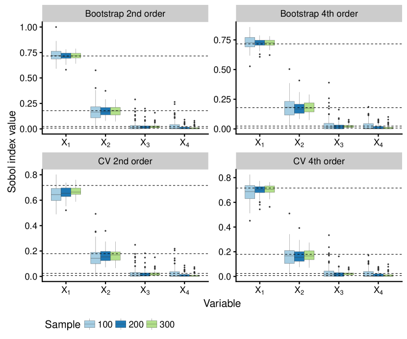
Figure 3: Estimated values from the 100 iterations for the g-Sobol model using the cross-validation and bootstrap procedures to estimate the bandwidth. Both methods were calculated using an Epanechnikov kernel of second and fourth order. The horizontal dashed lines represent the theoretical values for each Sobol index.

The Table 1 presents the bias and variance of $\widehat{S}_{i}^{\mathrm{Boot}}$ and $\widehat{S}_{i}^{\mathrm{CV}}$. Notice how the bias using a second order kernel with the bootstrap method is lower with respect to the cross-validation counterpart. If we use the fourth order kernel, the bias of the bootstrap method increases, while for the cross-validation remains under the true value of the Sobol index $S_{i}$. Recall our procedure over-fits the cross-validation procedure to reduce the bias. One disvantange of our procedure is a slightly increasing in the variance. In Figure 1 we observe how the variance oscillates among each iteration.

In the bottom of Table 1 we present the average raw distance between the bootstrap against the cross-validation estimators for $S_{i}$. The results show that in average $\widehat{S}_{i}^{\mathrm{Boot}}$ is over $\widehat{S}_{i}^{\mathrm{CV}}$ most of the cases. Figure 3 confirms this behavior.

		n = 100		n = 200		n = 300
	Variable	2nd order	4th order	2nd order	4th order	2nd order	4th order
$\mathrm{Bias}(\widehat{S}_{i}^{\mathrm{Boot}})$	$X_{1}$	0.0076	0.0112	-0.0021	0.0072	0.0015	0.0088
	$X_{2}$	-0.0052	0.0044	-0.0044	-0.0050	-0.0026	0.0010
	$X_{3}$	0.0057	0.0130	0.0000	-0.0015	-0.0010	-0.0007
	$X_{4}$	0.0221	0.0198	0.0047	0.0062	0.0028	0.0040
$\mathrm{Bias}(\widehat{S}_{i}^{\mathrm{CV}})$	$X_{1}$	-0.0700	-0.0356	-0.0581	-0.0176	-0.0476	-0.0120
	$X_{2}$	-0.0244	-0.0092	-0.0175	-0.0147	-0.0133	-0.0073
	$X_{3}$	0.0024	0.0099	-0.0020	-0.0027	-0.0028	-0.0018
	$X_{4}$	0.0181	0.0175	0.0036	0.0054	0.0019	0.0035
$\mathrm{Var}(\widehat{S}_{i}^{\mathrm{Boot}})$	$X_{1}$	0.0039	0.0031	0.0013	0.0011	0.0009	0.0008
	$X_{2}$	0.0089	0.0071	0.0030	0.0032	0.0023	0.0025
	$X_{3}$	0.0022	0.0036	0.0011	0.0007	0.0004	0.0002
	$X_{4}$	0.0025	0.0016	0.0004	0.0004	0.0002	0.0003
$\mathrm{Var}(\widehat{S}_{i}^{\mathrm{CV}})$	$X_{1}$	0.0047	0.0059	0.0019	0.0018	0.0012	0.0012
	$X_{2}$	0.0068	0.0065	0.0027	0.0030	0.0021	0.0024
	$X_{3}$	0.0017	0.0029	0.0009	0.0006	0.0004	0.0002
	$X_{4}$	0.0018	0.0013	0.0003	0.0004	0.0002	0.0003
$\mathbb{E}(\widehat{S}_{i}^{\mathrm{Boot}}-\widehat{S}_{i}^{\mathrm{CV}})$	$X_{1}$	0.0777	0.0467	0.0560	0.0248	0.0491	0.0208
	$X_{2}$	0.0192	0.0136	0.0131	0.0097	0.0108	0.0082
	$X_{3}$	0.0034	0.0031	0.0020	0.0012	0.0018	0.0011
	$X_{4}$	0.0040	0.0023	0.0011	0.0008	0.0008	0.0006

Table 1: Mean squared error over the 100 replications of the estimated against the theoretical values for the first four variables of the g-Sobol model. Here $\widehat{S}_{i}^{\mathrm{Boot}}$ and $\widehat{S}_{i}^{\mathrm{CV}}$ are the estimated Sobol indices using the Bootstrap and Cross-validation methods. The last four rows estimate the average distance between the Bootstrap and Cross-validation estimators.

Table 2 presents the median estimated bandwidths for the g-Sobol. The algorithm calculated the bandwidths using cross-validation and the bootstrap methods with second order Epanechnikov kernel. The results show us the over-fitting explained before, due to the choice of smaller bandwidths for the bootstrap algorithm. Here, there were values that did not converge to an optimal solution and the bandwidth $h$ tend to infinity. The phenomenon is due to the regression curve $\mathbb{E}[Y|X_{i}]$ is almost flat, causing that their variance stay in almost zero. For those examples, the non-parametric curve estimator represent only the mean of the data regarding $Y$.

Method	Bandwidth	$n=100$	$n=200$	$n=300$
Bootstrap	$h_{1}$	0.005	0.004	0.004
	$h_{2}$	0.012	0.009	0.008
	$h_{3}$	0.037	0.019	0.020
	$h_{4}$	0.130	0.066	0.032
Cross-validation	$h_{1}$	0.051	0.045	0.039
	$h_{2}$	0.096	0.079	0.065
	$h_{3}$	0.187	0.121	0.129
	$h_{4}$	0.373	0.226	0.168

Table 2: Median bandwidths estimated from the 100 iterations for the first four variable of the g-Sobol model.

5.2 Hydrologic application

One academic real case model to test the performance in sensitivity analysis is the dyke model. This model simplifies the 1D hydro-dynamical equations of Saint Venant under the assumptions of uniform and constant flow rate and large rectangular sections.

The following equations recreate the variable $S$ which measures the maximal annual overflow of the river (in meters) and the variable $C_{p}$ which is the associated cost (in millions of euros) of the dyke.

$$S =Z_{v}+H-H_{d}-C_{b}$$ (16)

$$\quad\text{with}\quad H=\left(\frac{Q}{BK_{s}\sqrt{\frac{Z_{m}-Z_{v}}{L}}}\right)$$

$$C_{p} =\bm{1}_{S>0}+\left[0.2+0.8\left(1-\exp{\frac{-1000}{S^{4}}}\right)\right]\bm{1}_{S\leq 0}$$ (17)

$$\qquad+\frac{1}{20}\left(H_{d}\bm{1}_{H_{d}>8}+8\bm{1}_{H_{d}\leq 8}\right)$$

Table 3 shows the inputs ($p=8$). Here $\bm{1}_{A}(x)$ is equal to 1 for $x\in A$ and 0 otherwise. The variable $H_{d}$ in Equation (16) is a design parameter for the Dyke’s height set as a $\mathrm{Uniform}(7,9)$.

In Equation (17), the first term is 1 million euros due to a flooding ($S>0$), the second term corresponds to the cost of the dyke maintenance ($S\leq 0$) and the third term is the construction cost related to the dyke. The latter cost is constant for a height of dyke less than 8 m and is growing like the dyke height otherwise.

Input	Description	Unit	Probability Distribution
$Q$	Maximal annual flowrate	m3/s	$\mathrm{Gumbel}(1013,558)$ truncated on [500, 3000]
$K_{s}$	Strickler coefficient	—	$\mathcal{N}(30,8)$ truncated on $\left[15,\infty\right)$
$Z_{v}$	River downstream level	m	$\mathrm{Triangular}(49,50,51)$
$Z_{m}$	River upstream level	m	$\mathrm{Triangular}(54,55,56)$
$H_{d}$	Dyke height	m	$\mathrm{Uniform}(7,9)$
$C_{b}$	Bank level	m	$\mathrm{Triangular}(55,55.5,56)$
$L$	Length of the river stretch	m	$\mathrm{Triangular}(4990,5000,5010)$
$B$	River width	m	$\mathrm{Triangular}(295,300,305)$

Table 3: Input variables and their probability distributions.

For a complete discussion about the model, their parameters and their meaning the reader can review Iooss and Lemaître, (2015), de Rocquigny, (2006) and their references.

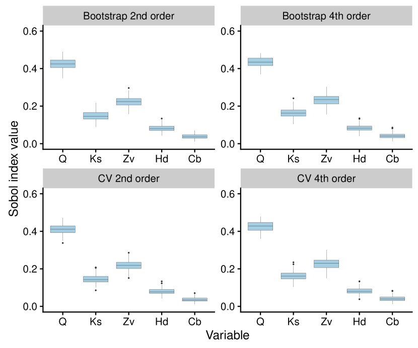
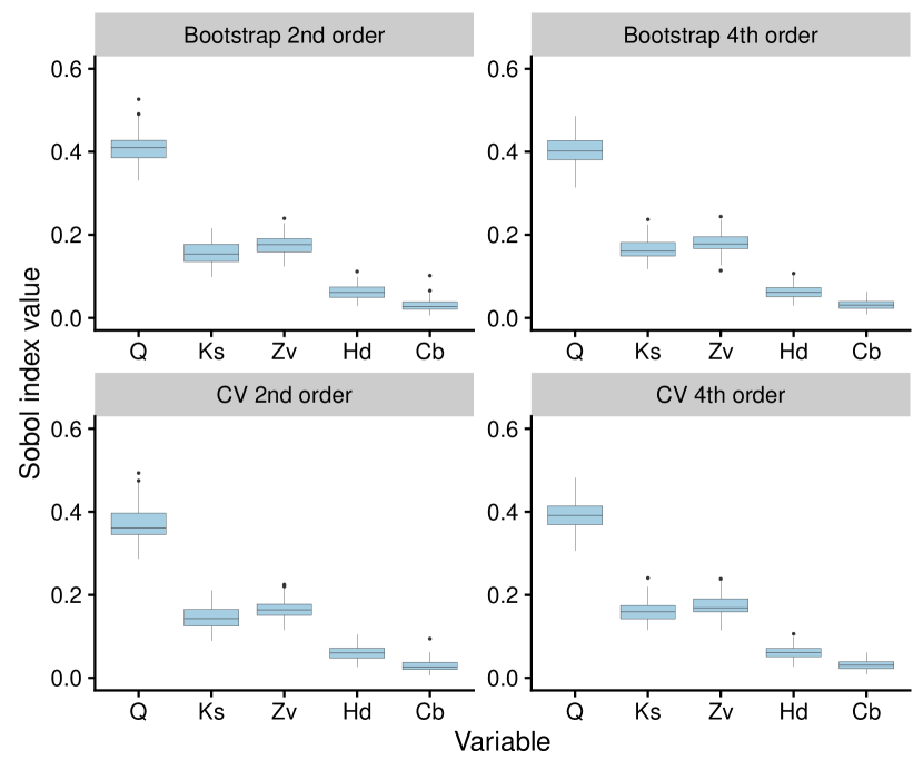
Figure 4: Estimated values from the 100 iterations for the output $S$ and $C_{p}$ in the Dyke model.

We generated 1000 observations for each input according to Table 3 and their respective values for $S$ and $C_{p}$. Figure 4 shows the result of simulations for the output $S$ and $C_{p}$ of the Dyke model using the cross-validation and bootstrap procedures.

For both output $S$ and $C_{p}$ we see that the variables in order of importance are $Q$, $Z_{v}$, $K_{s}$, $H_{d}$ and $C_{b}$. The rest of variables have values near to zero, and they provided insignificant impact to the output.

As reported in Table 4, we compared the values from our procedure against the reported by Iooss and Lemaître,. The values of the Sobol indices detect the influence of each variable compared with the classic Monte-Carlo and meta-models procedures. The exception is $H_{d}$, which in our case decreased to values near to $5\%$ against the reported values of $12.5\%-13.9\%$.

Indices (in %)	$Q$	$K_{s}$	$Z_{v}$	$H_{d}$	$C_{b}$
$S_{i}$ Monte-Carlo (Iooss)	35.5	15.9	18.3	12.5	3.8
$S_{i}$ Meta-model (Iooss)	38.9	16.8	18.8	13.9	3.7
$S_{i}$ Bootstrap	40.5	15.5	18.1	5.7	2.9
$S_{i}$ Cross-validation	37.2	14.6	17.2	5.5	2.8

Table 4: Comparison between the Sobol indices in the dyke model reported by Iooss and Lemaître, (2015) and our method. The Monte-Carlo and meta-model methods used samples of $10^{5}$. The bootstrap and cross-validation method used samples of $10^{3}$. In all cases the simulation repeated the experiment 100 times.

6 Conclusions

This paper presented an alternative way to estimate first order Sobol indices for the general model $Y=\varphi(X_{1},\ldots,X_{p})$. These indices are calculated using the formula $S_{i}=\mathrm{Var}(\mathbb{E}[Y|X_{i}])/\mathrm{Var}(Y)$. The method builds the regression curve $\mathbb{E}[Y|X_{i}]$ by a kernel non-parametric regression.

The least-square cross-validation procedure is a classic way to find the bandwidth. However, the literature presents cases where there exist a finite-sample bias on the model. One way to correct is increasing the number of samples. This method proposes a bootstrap algorithm to correct the bias, by first estimating the normalized residuals of the model and then recreating a bootstrap version of the response variable. With this new data, the algorithm estimates an empirical version of the least squared error. We call it Bootstrap Least-Square criterion and denoted $\mathrm{BLS}(h)$. The function $\mathrm{BLS}(h)$ finds its minimum in a value $\hat{h}_{boot}$.

The proposed algorithm over fits the regression curve $\mathbb{E}[Y|X_{i}]$, because it chooses a smaller bandwidth to increase the variability of the curve. It approximates the first order Sobol indices, but it could overestimate them when using fourth order kernels. The method proposed reduces the structural bias of caused for the non-parametric estimator. However, due to its construction the estimators have a slightly increased variance.

The function $\mathrm{BLS}$ was minimized using a Brent-type routine, implemented in the R function optimize. Due to the complexity of the target function, one future improvement to the algorithm is to use a global minimizer like simulated annealing to compare the results. In this scenario, we will expect a better choice of the bandwidths and observe a better adjust for the Sobol indices.

The method showed a consistent approximation to the Sobol indices only having the observational data available. In all cases, the non-parametric estimator using cross-validation and bootstrap approximate the influential variables in the $g$-Sobol and Dyke models.

We consider only the indices with simple interactions between one variable with respect the output. The higher order indices and total effects will remain for a further study. We will estimate the multivariate non-parametric surface for multiple variables. Then, we have to approximate the surface variability over some range. The latter step will be an interesting topic of study due to the numerical complexities.

Funding details

I acknowledge the financial support from the Vicerrectoría de Investigación de la Universidad de Costa Rica through the project 821–B4–257 administrated by the Escuela de Matemática and Centro de Investigaciones en Matemática Pura y Aplicada (CIMPA).

Disclosure statement

No potential conflict of interest was reported by the author.

References

- Alex Mara and Rakoto Joseph, (2008) Alex Mara, T. and Rakoto Joseph, O. (2008). Comparison of some efficient methods to evaluate the main effect of computer model factors. Journal of Statistical Computation and Simulation, 78(2):167–178.
- Baudin et al., (2016) Baudin, M., Boumhaout, K., Delage, T., Iooss, B., and Martinez, J.-M. (2016). Numerical stability of Sobol’ indices estimation formula. In 8th International Conference on Sensitivity Analysis of Model Output, pages 50–51, Reunion Island, France.
- Box and Draper, (1987) Box, G. E. P. and Draper, N. R. (1987). Empirical model-building and response surfaces. Wiley series in probability and mathematical statistics: Applied probability and statistics. John Wiley & Sons.
- Campolongo et al., (2011) Campolongo, F., Saltelli, A., and Cariboni, J. (2011). From screening to quantitative sensitivity analysis. A unified approach. Computer Physics Communications, 182(4):978–988.
- Carmichael et al., (1997) Carmichael, G. R., Sandu, A., and Potra, F. A. (1997). Sensitivity analysis for atmospheric chemistry models via automatic differentiation. Atmospheric Environment, 31(3):475–489.
- Cukier et al., (1978) Cukier, R., Levine, H., and Shuler, K. (1978). Nonlinear sensitivity analysis of multiparameter model systems. Journal of Computational Physics, 26(1):1–42.
- Cukier et al., (1973) Cukier, R. I., Fortuin, C. M., Shuler, K. E., Petschek, A. G., and Schaibly, J. H. (1973). Study of the sensitivity of coupled reaction systems to uncertainties in rate coefficients. I Theory. The Journal of Chemical Physics, 59(8):3873–3878.
- Cullen and Frey, (1999) Cullen, A. C. and Frey, H. C. (1999). Probabilistic Techniques in Exposure Assessment. Springer.
- de Rocquigny, (2006) de Rocquigny, É. (2006). La maîtrise des incertitudes dans un contexte industriel. 1re partie : une approche méthodologique globale basée sur des exemples. Journal de la société française de statistique, 147(3):33–71.
- Draper and Smith, (1981) Draper, N. R. and Smith, H. (1981). Applied regression analysis. Wiley, 2, illustr edition.
- Faraway and Jhun, (1990) Faraway, J. J. and Jhun, M. (1990). Bootstrap Choice of Bandwidth for Density Estimation. Journal of the American Statistical Association, 85(412):1119–1122.
- Goos, (2002) Goos, P. (2002). The Optimal Design of Blocked and Split-Plot Experiments, volume 164 of Lecture Notes in Statistics. Springer New York, New York, NY.
- Hansen, (2005) Hansen, B. E. (2005). Exact mean integrated squared error of higher order kernel estimators. Econometric Theory, 21(06):1031–1057.
- Hardle and Mammen, (1993) Hardle, W. and Mammen, E. (1993). Comparing Nonparametric Versus Parametric Regression Fits. The Annals of Statistics, 21(4):1926–1947.
- Härdle et al., (2004) Härdle, W., Werwatz, A., Müller, M., and Sperlich, S. (2004). Nonparametric and Semiparametric Models. Springer Series in Statistics. Springer Berlin Heidelberg, Berlin, Heidelberg.
- Hayfield and Racine, (2008) Hayfield, T. and Racine, J. S. (2008). Nonparametric Econometrics: The np Package. Journal of Statistical Software, 27(5):1–32.
- Iooss and Lemaître, (2015) Iooss, B. and Lemaître, P. (2015). A Review on Global Sensitivity Analysis Methods. In Dellino, G. and Meloni, C., editors, Uncertainty Management in Simulation-Optimization of Complex Systems: Algorithms and Applications, pages 101–122. Springer US, Boston, MA.
- Ishigami and Homma, (1990) Ishigami, T. and Homma, T. (1990). An importance quantification technique in uncertainty analysis for computer models. In Uncertainty Modeling and Analysis, 1990. Proceedings., First International Symposium on, pages 398–403. IEEE, IEEE Comput. Soc. Press.
- Janon et al., (2014) Janon, A., Klein, T., Lagnoux, A., Nodet, M., and Prieur, C. (2014). Asymptotic normality and efficiency of two Sobol index estimators. ESAIM: Probability and Statistics, 18(3):342–364.
- Jansen, (1999) Jansen, M. J. (1999). Analysis of variance designs for model output. Computer Physics Communications, 117(1-2):35–43.
- Loubes et al., (2019) Loubes, J.-M., Marteau, C., and Solís, M. (2019). Rates of convergence in conditional covariance matrix with nonparametric entries estimation. Communications in Statistics - Theory and Methods.
- Makowski et al., (2006) Makowski, D., Naud, C., Jeuffroy, M.-H., Barbottin, A., and Monod, H. (2006). Global sensitivity analysis for calculating the contribution of genetic parameters to the variance of crop model prediction. Reliability Engineering & System Safety, 91(10-11):1142–1147.
- Myer and Montgomery, (2002) Myer, R. and Montgomery, D. (2002). Response Surface Methodology: Process and Product Optimization Using Designed Experiments. Wiley, New York.
- Oakley and O’Hagan, (2004) Oakley, J. E. and O’Hagan, A. (2004). Probabilistic sensitivity analysis of complex models: a Bayesian approach. Journal of the Royal Statistical Society: Series B (Statistical Methodology), 66(3):751–769.
- Owen, (2013) Owen, A. B. (2013). Better estimation of small sobol’ sensitivity indices. ACM Transactions on Modeling and Computer Simulation, 23(2):1–17.
- Padgett and Thombs, (1986) Padgett, W. J. and Thombs, L. a. (1986). Smooth nonparametric quantile estimation under censoring: simulations and bootstrap methods. Communications in Statistics - Simulation and Computation, 15(4):1003–1025.
- R. and J.L, (2012) R., P. and J.L, D. (2012). Statistics: The Exploration and Analysis of Data. Cole, Pacific Grove, CA, pages 1–817.
- R Core Team, (2018) R Core Team (2018). R: A Language and Environment for Statistical Computing. R Foundation for Statistical Computing, Vienna, Austria. \urlhttps://www.R-project.org/.
- Racine, (2001) Racine, J. (2001). Bias-Corrected Kernel Regression. Journal of Quantitative Economics, 17(1):25–42.
- Rall, (1980) Rall, L. B. (1980). Applications of software for automatic differentiation in numerical computation. Springer.
- Ratto and Pagano, (2010) Ratto, M. and Pagano, A. (2010). Using recursive algorithms for the efficient identification of smoothing spline ANOVA models. AStA Advances in Statistical Analysis, 94(4):367–388.
- Romano, (1988) Romano, J. P. (1988). On Weak Convergence and Optimality of Kernel Density Estimates of the Mode. The Annals of Statistics, 16(2):629–647.
- Saltelli, (2002) Saltelli, A. (2002). Making best use of model evaluations to compute sensitivity indices. Computer Physics Communications, 145(2):280–297.
- Saltelli et al., (2000) Saltelli, A., Chan, K., and Scott, E. (2000). Sensitivity analysis, volume 134. Wiley New York.
- Saltelli et al., (2009) Saltelli, A., Chan, K., and Scott, E. M. (2009). Sensitivity Analysis. Wiley, New York, 1 edition edition.
- Saltelli et al., (2007) Saltelli, A., Ratto, M., Andres, T., Campolongo, F., Cariboni, J., Gatelli, D., Saisana, M., and Tarantola, S. (2007). Global Sensitivity Analysis. The Primer. John Wiley & Sons, Ltd, Chichester, UK.
- Sobol’, (2001) Sobol’, I. (2001). Global sensitivity indices for nonlinear mathematical models and their Monte Carlo estimates. Mathematics and Computers in Simulation, 55(1-3):271–280.
- Sobol’ et al., (2007) Sobol’, I., Tarantola, S., Gatelli, D., Kucherenko, S., and Mauntz, W. (2007). Estimating the approximation error when fixing unessential factors in global sensitivity analysis. Reliability Engineering & System Safety, 92(7):957–960.
- Sobol’, (1993) Sobol’, I. M. (1993). Sensitivity Estimates for Nonlinear Mathematical Models. Mathematical Modeling and Computational experiment, 1(4):407–414.
- Touati, (2016) Touati, T. (2016). Confidence intervals for Sobol’ indices. In 8th International Conference on Sensitivity Analysis of Model Output, pages 93–94, Reunion Island, France.
- Tsybakov, (2009) Tsybakov, A. B. (2009). Introduction to Nonparametric Estimation. Springer Series in Statistics. Springer New York, New York, NY, 1st editio edition.
- Zhao et al., (2017) Zhao, Y.-Y., Lin, J.-G., and Wang, H.-X. (2017). Robust bootstrap estimates in heteroscedastic semi-varying coefficient models and applications in analyzing australia cpi data. Communications in Statistics - Simulation and Computation, 46(4):2638–2653.
- Zhu and Fang, (1996) Zhu, L.-X. X. and Fang, K.-T. T. (1996). Asymptotics for kernel estimate of sliced inverse regression. The Annals of Statistics, 24(3):1053–1068.