Efficient Loss-Based Decoding on Graphs for Extreme Classification

Abstract

In extreme classification problems, learning algorithms are required to map instances to labels from an extremely large label set. We build on a recent extreme classification framework with logarithmic time and space [19], and on a general approach for error correcting output coding (ECOC) with loss-based decoding [1], and introduce a flexible and efficient approach accompanied by theoretical bounds. Our framework employs output codes induced by graphs, for which we show how to perform efficient loss-based decoding to potentially improve accuracy. In addition, our framework offers a tradeoff between accuracy, model size and prediction time. We show how to find the sweet spot of this tradeoff using only the training data. Our experimental study demonstrates the validity of our assumptions and claims, and shows that our method is competitive with state-of-the-art algorithms.

1 Introduction

Multiclass classification is the task of assigning instances with a category or class from a finite set. Its numerous applications range from finding a topic of a news item, via classifying objects in images, via spoken words detection, to predicting the next word in a sentence. Our ability to solve multiclass problems with larger and larger sets improves with computation power. Recent research focuses on extreme classification where the number of possible classes $K$ is extremely large.

In such cases, previously developed methods, such as One-vs-One (OVO) [17], One-vs-Rest (OVR) [9] and multiclass SVMs  [34, 6, 11, 25], that scale linearly in the number of classes $K$, are not feasible. These methods maintain too large models, that cannot be stored easily. Moreover, their training and inference times are at least linear in $K$, and thus do not scale for extreme classification problems.

Recently, Jasinska and Karampatziakis [19] proposed a Log-Time Log-Space (LTLS) approach, representing classes as paths on graphs. LTLS is very efficient, but has a limited representation, resulting in an inferior accuracy compared to other methods. More than a decade earlier, Allwein et al. [1] presented a unified view of error correcting output coding (ECOC) for classification, as well as the loss-based decoding framework. They showed its superiority over Hamming decoding, both theoretically and empirically.

In this work we build on these two works and introduce an efficient (i.e. $O(\log K)$ time and space) loss-based learning and decoding algorithm for any loss function of the binary learners’ margin. We show that LTLS can be seen as a special case of ECOC. We also make a more general connection between loss-based decoding and graph-based representations and inference. Based on the theoretical framework and analysis derived by [1] for loss-based decoding, we gain insights on how to improve on the specific graphs proposed in LTLS by using more general trellis graphs – which we name Wide-LTLS (W-LTLS). Our method profits from the best of both worlds: better accuracy as in loss-based decoding, and the logarithmic time and space of LTLS. Our empirical study suggests that by employing coding matrices induced by different trellis graphs, our method allows tradeoffs between accuracy, model size, and inference time, especially appealing for extreme classification.

2 Problem setting

We consider multiclass classification with $K$ classes, where $K$ is very large. Given a training set of $m$ examples $\left(x_{i},y_{i}\right)$ for $x_{i}\in\mathcal{X}\subseteq\mathbb{R}^{d}$ and $y_{i}\in\mathcal{Y}=\{1,...,K\}$ our goal is to learn a mapping from $\mathcal{X}$ to $\mathcal{Y}$. We focus on the 0/1 loss and evaluate the performance of the learned mapping by measuring its accuracy on a test set – i.e. the fraction of instances with a correct prediction. Formally, the accuracy of a mapping $h:\mathcal{X}\rightarrow\mathcal{Y}$ on a set of $n$ pairs, $\left\{\left(x_{i},y_{i}\right)\right\}_{i=1}^{n}$, is defined as $\frac{1}{n}\sum_{i=1}^{n}\mathbf{1}_{h(x_{i})=y_{i}}$, where $\mathbf{1}_{z}$ equals $1$ if the predicate $z$ is true, and $0$ otherwise.

3 Error Correcting Output Coding (ECOC)

Dietterich and Bakiri [14] employed ideas from coding theory [23] to create Error Correcting Output Coding (ECOC) – a reduction from a multiclass classification problem to multiple binary classification subproblems. In this scheme, each class is assigned with a (distinct) binary codeword of $\ell$ bits (with values in $\{-1,+1\}$). The $K$ codewords create a matrix $M\in\left\{-1,+1\right\}^{K\times{\ell}}$ whose rows are the codewords and whose columns induce $\ell$ partitions of the classes into two subsets. Each of these partitions induces a binary classification subproblem. We denote by $M_{k}$ the $k$th row of the matrix, and by $M_{k,j}$ its $(k,j)$ entry. In the j$th$ partition, class $k$ is assigned with the binary label $M_{k,j}$.

ECOC introduces redundancy in order to acquire error-correcting capabilities such as a minimum Hamming distance between codewords. The Hamming distance between two codewords $M_{a},M_{b}$ is defined as $\rho(a,b)\triangleq\sum_{j=1}^{\ell}\frac{1-M_{a,j}M_{b,j}}{2}$, and the minimum Hamming distance of $M$ is $\rho=\min_{a\neq{b}}\rho(a,b)$. A high minimum distance of the coding matrix potentially allows overcoming binary classification errors during inference time.

At training time, this scheme generates $\ell$ binary classification training sets of the form $\left\{x_{i},M_{y_{i},j}\right\}^{m}_{i=1}$ for $j=1,\dots,\ell$, and executes some binary classification learning algorithm that returns $\ell$ classifiers, each trained on one of these sets. We assume these classifiers are margin-based, that is, each classifier is a real-valued function, $f_{j}:\mathcal{X}\to\mathbb{R}$, whose binary prediction for an input $x$ is ${\rm sign}\left(f_{j}\left(x\right)\right)$. The binary classification learning algorithm defines a margin-based loss $L:\mathbb{R}\rightarrow\mathbb{R}_{+}$, and minimizes the average loss over the induced set. Formally, $f_{j}=\arg\min_{f\in\mathcal{F}}\frac{1}{m}\sum_{i=1}^{m}L\left(M_{y_{i},j}f\left(x_{i}\right)\right)$, where $\mathcal{F}$ is a class of functions, such as the class of bounded linear functions. Few well known loss functions are the hinge loss $L(z)\triangleq\max\left(0,1-z\right)$, used by SVM, its square, the log loss $L\left(z\right)\triangleq\log\left(1+e^{-z}\right)$ used in logistic regression, and the exponential loss $L\left(z\right)\triangleq e^{-z}$ used in AdaBoost [30].

Once these classifiers are trained, a straightforward inference is performed. Given an input $x$, the algorithm first applies the $\ell$ functions on $x$ and computes a $\{\pm 1\}$-vector of size $\ell$, that is $\left({\rm sign}\left(f_{1}\left(x\right)\right)\dots\rm sign\left(f_{\ell}\left(x\right)\right)\right)$. Then, the class $k$ which is assigned to the codeword closest in Hamming distance to this vector is returned. This inference scheme is often called Hamming decoding.

The Hamming decoding uses only the binary prediction of the binary learners, ignoring the confidence each learner has in its prediction per input. Allwein et al. [1] showed that this margin or confidence holds valuable information for predicting a class $y\in\mathcal{Y}$, and proposed the loss-based decoding framework for ECOC. In loss-based decoding, the margin is incorporated via the loss function $L(z)$. Specifically, the class predicted is the one minimizing the total loss

$$k^{*}=\arg\min_{k}\sum_{j=1}^{\ell}L\left(M_{k,j}f_{j}\left(x\right)\right)~{}.$$ (1)

They [1] also developed error bounds and showed theoretically and empirically that loss-based decoding outperforms Hamming decoding.

One drawback of their method is that given a loss function $L$, loss-based decoding requires an exhaustive evaluation of the total loss for each codeword $M_{k}$ (each row of the coding matrix). This implies a decoding time at least linear in $K$, making it intractable for extreme classification. We address this problem below.

4 LTLS

A recent extreme classification approach, proposed by Jasinska and Karampatziakis [19], performs training and inference in time and space logarithmic in $K$, by embedding the $K$ classes into $K$ paths of a directed-acyclic trellis graph $T$, built compactly with $\ell=\mathcal{O}\left(\log{K}\right)$ edges. We denote the set of vertices $V$ and set of edges $E$. A multiclass model is defined using $\ell$ functions from the feature space to the reals, $w_{j}\left(x\right)$, one function per edge in $E=\{e_{j}\}_{j=1}^{\ell}$. Given an input, the algorithm assigns weights to the edges, and computes the heaviest path using the Viterbi [32] algorithm in $\mathcal{O}\left(\left|E\right|\right)=\mathcal{O}\left(\log{K}\right)$ time. It then outputs the class (from $\mathcal{Y}$) assigned to the heaviest path.

Jasinska and Karampatziakis [19] proposed to train the model in an online manner. The algorithm maintains $\ell$ functions $f_{j}(x)$ and works in rounds. In each training round a specific input-output pair $\left(x_{i},y_{i}\right)$ is considered, the algorithm performs inference using the $\ell$ functions to predict a class $\hat{y}_{i}$, and the functions $f_{j}(x)$ are modified to improve the overall prediction for $x_{i}$ according to $y_{i},\hat{y}_{i}$. The inference performed during train and test times, includes using the obtained functions $f_{j}(x)$ to compute the weights $w_{j}(x)$ of each input, by simply setting $w_{j}(x)=f_{j}(x)$. Specifically, they used margin-based learning algorithms, where $f_{j}(x)$ is the margin of a binary prediction.

Our first contribution is the observation that the LTLS approach can be thought of as an ECOC scheme, in which the codewords (rows) represent paths in the trellis graph, and the columns correspond to edges on the graph. Figure 2 illustrates how a codeword corresponds to a path on the graph.

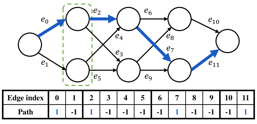
Figure 1: Path codeword representation. An entry containing 1 means that the corresponding edge is a part of the illustrated bold blue path. The green dashed rectangle shows a vertical slice.

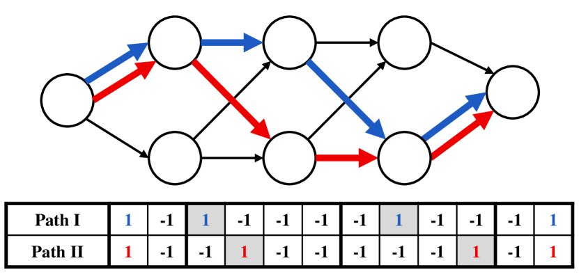
Figure 2: Two closest paths. Predicting Path II (red) instead of I (blue), will result in a prediction error. The Hamming distance between the corresponding codewords is 4. The highlighted entries correspond to the 4 disagreement edges.

It might seem like this approach can represent only numbers of classes $K$ which are powers of $2$. However, in Appendix C.1 we show how to create trellis graphs with exactly $K$ paths, for any $K\in\mathbb{N}$.

4.1 Path assignment

LTLS requires a bijective mapping between paths to classes and vice versa. It was proposed in [19] to employ a greedy assignment policy suitable for online learning, where during training, a sample whose class is yet unassigned with a path, is assigned with the heaviest unassigned path. One could also consider a naive random assignment between paths and classes.

4.2 Limitations

The elegant LTLS construction suffers from two limitations:

1. Difficult induced binary subproblems: The induced binary subproblems are hard, especially when learned with linear classifiers. Each path uses one of four edges between every two adjacent vertical slices. Therefore, each edge is used by $\frac{1}{4}$ of the classes, inducing a $\frac{1}{4}K$-vs-$\frac{3}{4}K$ subproblem. Similarly, the edges connected to the source or sink induce $\frac{1}{2}K$-vs-$\frac{1}{2}K$ subproblems. In both cases classes are split into two groups, almost arbitrarily, with no clear semantic interpretation for that partition. For comparison, in 1-vs-Rest (OVR) the induced subproblems are considered much simpler as they require classifying only one class vs the rest (meaning they are much less balanced).

2. Low minimum distance: In the LTLS trellis architecture, every path has another (closest) path within 2 edge deletions and 2 edge insertions (see Figure 2). Thus, the minimum Hamming distance in the underlying coding matrix is restrictively small: $\rho=4$, which might imply a poor error correcting capability. The OVR coding matrix also suffers from a small minimum distance ($\rho=2$), but as we explained, the induced subproblems are very simple, allowing a higher classification accuracy in many cases.

We focus on improving the multiclass accuracy by tackling the first limitation, namely making the underlying binary subproblems easier. Addressing the second limitation is deferred to future work.

5 Efficient loss-based decoding

We now introduce another contribution – a new algorithm performing efficient loss-based decoding (inference) for any loss function by exploiting the structure of trellis graphs. Similarly to [19], our decoding algorithm performs inference in two steps. First, it assigns (per input $x$ to be classified) weights $\left\{w_{j}\left(x\right)\right\}_{j=1}^{\ell}$ to the edges $\left\{e_{j}\right\}_{j=1}^{\ell}$ of the trellis graph. Second, it finds the shortest path (instead of the heaviest) $P_{k^{*}}$ by an efficient dynamic programming (Viterbi) algorithm and predicts the class $k^{*}$. Unlike [19], our strategy for assigning edge weights ensures that for any class $k$, the weight of the path assigned to this class, $w\left(P_{k}\right)\triangleq\sum_{j:e_{j}\in P_{k}}w_{j}\left(x\right)$, equals the total loss $\sum_{j=1}^{\ell}L\left(M_{k,j}f_{j}\left(x\right)\right)$ for the classified input $x$. Therefore, finding the shortest path on the graph is equivalent to minimizing the total loss, which is the aim in loss-based decoding. In other words, we design a new weighting scheme that links loss-based decoding to the shortest path in a graph.

We now describe our algorithm in more detail for the case when the number of classes $K$ is a power of 2 (see Appendix C.2 for extension to arbitrary $K$). Consider a directed edge $e_{j}\in{E}$ and denote by $\left(u_{j},v_{j}\right)$ the two vertices it connects. Denote by $S\left(e_{j}\right)$ the set of edges outgoing from the same vertical slice as $e_{j}$. Formally, $S\left(e_{j}\right)=\left\{\left(u,u^{\prime}\right):\delta\left(u\right)=\delta\left(u_{j}\right)\right\}$, where $\delta\left(v\right)$ is the shortest distance from the source vertex to $v$ (in terms of number of edges). For example, in Figure 2, $S\left(e_{0}\right)=S\left(e_{1}\right)=\left\{e_{0},e_{1}\right\}$, $S\left(e_{2}\right)=S\left(e_{3}\right)=S\left(e_{4}\right)=S\left(e_{5}\right)=\left\{e_{2},e_{3},e_{4},e_{5}\right\}$. Given a loss function $L\left(z\right)$ and an input instance $x$, we set the weight $w_{j}$ for edge $e_{j}$ as following,

$$w_{j}\left(x\right)=L\left(1\times f_{j}(x)\right)+\sum_{j{{}^{\prime}}:e_{j^{\prime}}\in S\left(e_{j}\right)\backslash\left\{e_{j}\right\}}L\left((-1)\times f_{j^{\prime}}(x)\right)~{}.$$ (2)

For example, in Figure 2 we have,

$$w_{0}\left(x\right)= ~{}L\left(1\times f_{0}(x)\right)+L\left(\left(-1\right)\times f_{1}(x)\right)$$

$$w_{2}\left(x\right)= ~{}L\left(1\times f_{2}(x)\right)+L\left(\left(-1\right)\times f_{3}(x)\right)+L\left(\left(-1\right)\times f_{4}(x)\right)+L\left((-1)\times f_{5}(x)\right)~{}.$$

The next theorem states that for our choice of weights, finding the shortest path in the weighted graph is equivalent to loss-based decoding. Thus, algorithmically we can enjoy fast decoding (i.e. inference), and statistically we can enjoy better performance by using loss-based decoding.

Theorem 1

Let $L\left(z\right)$ be any loss function of the margin. Let $T$ be a trellis graph with an underlying coding matrix $M$. Assume that for any $x\in\mathcal{X}$ the edge weights are calculated as in Eq. (2). Then, the weight of any path $P_{k}$ equals to the loss suffered by predicting its corresponding class $k$, i.e. $w(P_{k})=\sum_{j=1}^{\ell}L\left(M_{k,j}f_{j}(x)\right)$.

The proof appears in Appendix A. In the next lemma we claim that LTLS decoding is a special case of loss-based decoding with the squared loss function. See Appendix B for proof.

Lemma 2

Denote the squared loss function by $L_{sq}(z)\triangleq\left(1-z\right)^{2}$. Given a trellis graph represented using a coding matrix $M\in\{-1,+1\}^{K\times\ell}$, and $\ell$ functions $f_{j}\left(x\right)$, for $j=1\dots\ell$, the decoding method of LTLS (mentioned in Section 4) is a special case of loss-based decoding with the squared loss, that is $\arg\max_{k}w\left(P_{k}\right)=\arg\min_{k}\left\{\sum_{j}L_{sq}\left(M_{k,j}f_{j}\left(x\right)\right)\right\}~{}.$

We next build on the framework of [1] to design graphs with a better multiclass accuracy.

6 Wide-LTLS (W-LTLS)

Allwein et al. [1] derived error bounds for loss-based decoding with any convex loss function $L$. They showed that the training multiclass error with loss-based decoding is upper bounded by:

$$\frac{\ell\times\varepsilon}{\rho\times{L(0)}}$$ (3)

where $\rho$ is the minimum Hamming distance of the code and

$$\varepsilon=\frac{1}{m\ell}\sum_{i=1}^{m}{\sum_{j=1}^{\ell}{L\left(M_{y_{i},j}f_{j}{\left(x_{i}\right)}\right)}}$$ (4)

is the average binary loss on the training set of the learned functions $\{f_{j}\}_{j=1}^{\ell}$ with respect to a coding matrix $M$ and a loss $L$. One approach to reduce the bound, and thus hopefully also the multiclass training error (and under some conditions also the test error) is to reduce the total error of the binary problems $\ell\times\varepsilon$. We now show how to achieve this by generalizing the LTLS framework to a more flexible architecture which we call W-LTLS .

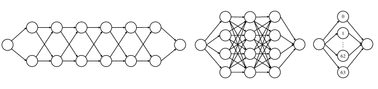
Figure 3: Different graphs for $K=64$ classes. From left to right: the LTLS graph with a slice width of $b=2$, W-LTLS with $b=4$, and the widest W-LTLS graph with $b=64$, corresponding to OVR.

Motivated by the error bound of [1], we propose a generalization of the LTLS model. By increasing the slice width of the trellis graph, and consequently increasing the number of edges between adjacent vertical slices, the induced subproblems become less balanced and potentially easier to learn (see Remark 2). For simplicity we choose a fixed slice width $b\in\left\{2,\dots,K\right\}$ for the entire graph (e.g. see Figure 3). In such a graph, most of the induced subproblems are $\frac{1}{b^{2}}K$-vs-rest (corresponding to edges between adjacent slices) and some are $\frac{1}{b}K$-vs-rest (the ones connected to the source or to the sink). As $b$ increases, the graph representation becomes less compact and requires more edges, i.e. $\ell$ increases. However, the induced subproblems potentially become easier, improving the multiclass accuracy. This suggests that our model allows an accuracy vs model size tradeoff.

In the special case where $b=K$ we get the widest graph containing $2K$ edges (see Figure 3). All the subproblems are now $1$-vs-rest: the $k$th path from the source to the sink contains two edges (one from the source and one to the sink) which are not a part of any other path. Thus, the corresponding two columns in the underlying coding matrix are identical – having $1$ at their $k$th entry and $\left(-1\right)$ at the rest. This implies that the distinct columns of the matrix could be rearranged as the diagonal coding matrix corresponding to OVR, making our model when $b=K$ an implementation of OVR.

In Section 7 we show empirically that W-LTLS improves the multiclass accuracy of LTLS. In Appendix E.2 we show that the binary subproblems indeed become easier, i.e. we observe a decrease in the average binary loss $\varepsilon$, lowering the bound in (3). Note that the denominator $\rho\times L\left(0\right)$ is left untouched – the minimum distance of the coding matrices corresponding to different architectures of W-LTLS is still 4, like in the original LTLS model (see Section 4.2).

6.1 Time and space complexity analysis

W-LTLS requires training and storing a binary learner for every edge. For most linear classifiers (with $d$ parameters each) we get a total model size complexity and an inference time complexity of $\mathcal{O}\left(d\left|E\right|\right)=\mathcal{O}\left(d\frac{b^{2}}{\log{b}}\log{K}\right)$ (see Appendix D for further details). Moreover, many extreme classification datasets are sparse – the average number of non-zero features in a sample is $d_{e}\ll d$. The inference time complexity thus decreases to $\mathcal{O}\left(d_{e}\frac{b^{2}}{\log{b}}\log{K}\right)$.

This is a significant advantage: while inference with loss-based decoding for general matrices requires $\mathcal{O}\left(d_{e}\ell+K\ell\right)$ time, our model performs it in only $\mathcal{O}\left(d_{e}\ell+\ell\right)=\mathcal{O}\left(d_{e}\ell\right)$.

Since training requires learning $\ell$ binary subproblems, the training time complexity is also sublinear in $K$. These subproblems can be learned separately on $\ell$ cores, leading to major speedups.

6.2 Wider graphs induce sparse models

The high sparsity typical to extreme classification datasets (e.g. the Dmoz dataset has $d=833,484$ features, but on average only $d_{e}=174$ of them are non-zero), is heavily exploited by previous works such as PD-Sparse [15], PPDSparse [35], and DiSMEC [2], which all learn sparse models.

Indeed, we find that for sparse datasets, our algorithm typically learns a model with a low percentage of non-zero weights. Moreover, the percentage of non-zero decreases significantly as the slice width $b$ is increased (see Appendix E.6). This allows us to employ a simple post-pruning of the learned weights. For some threshold value $\lambda$, we set to zero all learned weights in $\left[-\lambda,\lambda\right]$, yielding a sparse model. Similar approaches were taken by [2, 19, 15] either explicitly or implicitly.

In Section 7.3 we show that the above scheme successfully yields highly sparse models.

7 Experiments

We test our algorithms on 5 extreme multiclass datasets previously used in [15], having approximately $10^{2}$, $10^{3}$, and $10^{4}$ classes (see Table 1 in Appendix E.1). We use AROW [10] to train the binary functions $\left\{f_{j}\right\}_{j=1}^{\ell}$ of W-LTLS. Its online updates are based on the squared hinge loss $L_{SH}\left(z\right)\triangleq\left(\max\left(0,1-z\right)\right)^{2}$. For each dataset, we build wide graphs with multiple slice widths. For each configuration (dataset and graph) we perform five runs using random sample shuffling on every epoch, and a random path assignment (as explained in Section 4.1, unlike the greedy policy used in [19]), and report averages over these five runs. Unlike [19], we train the $\ell$ binary learners independently rather than in a joint (structured) manner. This allows parallel independent training, as common for training binary learners for ECOC, with no need to perform full multiclass inference during training.

7.1 Loss-based decoding

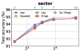
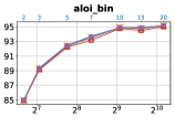
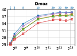
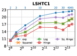
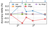
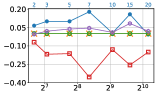
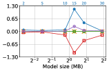
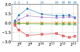
Figure 4: First row: Multiclass test accuracy as a function of the model size (MBytes) for loss-based decoding with different loss functions. Second row: Relative increase in multiclass test accuracy compared to decoding with the squared loss used implicitly in LTLS. The secondary x-axes (top axes, blue) indicate the slice widths ($b$) used for the W-LTLS trellis graphs.

We run W-LTLS with different loss functions for loss-based decoding: the exponential loss, the squared loss (used by LTLS, see Lemma 2), the log loss, the hinge loss, and the squared hinge loss.

The results appear in Figure 4. We observe that decoding with the exponential loss works the best on all five datasets. For the two largest datasets (Dmoz and LSHTC1) we report significant accuracy improvement when using the exponential loss for decoding in graphs with large slice widths ($b$), over the squared loss used implicitly by LTLS. Indeed, for these larger values of $b$, the subproblems are easier (see Appendix E.2 for detailed analysis). This should result in larger prediction margins $\left|f_{j}\left(x\right)\right|$, as we indeed observe empirically (shown in Appendix E.4). The various loss functions $L\left(z\right)$ differ significantly for $z\ll 0$, potentially explaining why we find larger accuracy differences as $b$ increases when decoding with different loss functions.

7.2 Multiclass test accuracy

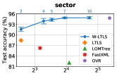
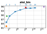
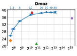
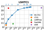
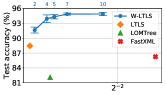
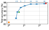
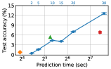
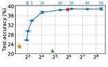
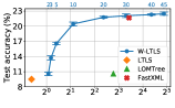
Figure 5: First row: Multiclass test accuracy vs model size. Second row: Multiclass test accuracy vs prediction time. A 95% confidence interval is shown for the results of W-LTLS.

We compare the multiclass test accuracy of W-LTLS (using the exponential loss for decoding) to the same baselines presented in [19]. Namely we compare to LTLS [19], LOMTree [7] (results quoted from [19]), FastXML [29] (run with the default parameters on the same computer as our model), and OVR (binary learners trained using AROW). For convenience, the results are also presented in a tabular form in Appendix E.5.

7.2.1 Accuracy vs Model size

The first row of Figure 5 (best seen in color) summarizes the multiclass accuracies vs model size.

Among the four competitors, LTLS enjoys the smallest model size, LOMTree and FastXML have larger model sizes, and OVR is the largest. LTLS achieves lower accuracies than LOMTree on two datasets, and higher ones on the other two. OVR enjoys the best accuracy, yet with a price of model size. For example, in Dmoz, LTLS achieves $23\%$ accuracy vs $35.5\%$ of OVR, though the model size of the latter is $\times 200$ larger than of the former.

In all five datasets, an increase in the slice width of W-LTLS (and consequently in the model size) translates almost always to an increase in accuracy. Our model is often better or competitive with the other algorithms that have logarithmic inference time complexity (LTLS, LOMTree, FastXML), and also competitive with OVR in terms of accuracy, while we still enjoy much smaller model sizes.

For the smallest model sizes of W-LTLS (corresponding to $b=2$), our trellis graph falls back to the one of LTLS. The accuracies gaps between these two models may be explained by the different binary learners the experiments were run with – LTLS used averaged Perceptron as the binary learner whilst we used AROW. Also, LTLS was trained in a structured manner with a greedy path assignment policy while we trained every binary function independently with a random path assignment policy (see Section 6.1). In our runs we observed that independent training achieves accuracy competitive with to structured online training, while usually converging much faster. It is interesting to note that for the imageNet dataset the LTLS model cannot fit the data, i.e the training error is close to 1 and the test accuracy is close to 0. The reason is that the binary subproblems are very hard, as was also noted by [19]. By increasing the slice width ($b$), the W-LTLS model mitigates this underfitting problem, still with logarithmic time and space complexity.

We also observe in the first row of Figure 5 that there is a point where the multiclass test accuracy of W-LTLS starts to saturate (except for imageNet). Our experiments show that this point can be found by looking at the training error and its bound only. We thus have an effective way to choose the optimal model size for the dataset and space/time budget at hand by performing model selection (width of the graph in our case) using the training error bound only (see detailed analysis in Appendix E.2 and Appendix E.3).

7.2.2 Accuracy vs Prediction time

In the second row of Figure 5 we compare prediction (inference) time of W-LTLS to other methods. LTLS enjoys the fastest prediction time, but suffers from low accuracy. LOMTree runs slower than LTLS, but sometimes achieves better accuracy. Despite being implemented in Python, W-LTLS is competitive with FastXML, which is implemented in C++.

7.3 Exploiting the sparsity of the datasets

We now demonstrate that the post-pruning proposed in Section 6.2, which zeroes the weights in $\left[-\lambda,\lambda\right]$, is highly beneficial. Since imageNet is not sparse at all, we do not consider it in this section.

We tune the threshold $\lambda$ so that the degradation in the multiclass validation accuracy is at most $1\%$ (tuning the threshold is done after the cumbersome learning of the weights, and does not require much time).

In Figure 6 we plot the multiclass test accuracy versus model size for the non-sparse W-LTLS, as well as the sparse W-LTLS after pruning the weights as explained above. We compare ourselves to the aforementioned sparse competitors: DiSMEC, PD-Sparse, and PPDSparse (all results quoted from [35]). Since the aforementioned FastXML [29] also exploits sparsity to reduce the size of the learned trees, we consider it here as well (we run the code supplied by the authors for various numbers of trees). For convenience, all the results are also presented in a tabular form in Appendix E.6.

We observe that our method can induce very sparse binary learners with a small degradation in accuracy. In addition, as expected, the wider the graphs (larger $b$), the more beneficial is the pruning. Interestingly, while the number of parameters increases as the graphs become wider, the actual storage space for the pruned sparse models may even decrease. This phenomenon is observed for the sector and aloi.bin datasets.

Finally, we note that although PD-Sparse [15] and DiSMEC [2] perform better on some model size regions of the datasets, their worse case space requirement during training is linear in the number of classes $K$, whereas our approach guarantees (adjustable) logarithmic space for training.

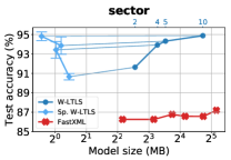
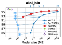
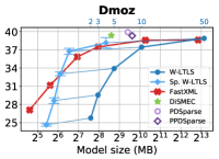
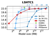
Figure 6: Multiclass test accuracy vs model size for sparse models. Lines between two W-LTLS plots connect the same models before and after the pruning. The secondary x-axes (top axes, blue) indicate the slice widths ($b$) used for the (unpruned) W-LTLS trellis graphs.

8 Related work

Extreme classification was studied extensively in the past decade. It faces unique challenges, amongst which is the model size of its designated learning algorithms. An extremely large model size often implies long training and test times, as well as excessive space requirements. Also, when the number of classes $K$ is extremely large, the inference time complexity should be sublinear in $K$ for the classifier to be useful.

The Error Correcting Output Coding (ECOC) (see Section 3) approach seems promising for extreme classification, as it potentially allows a very compact representation of the label space with $K$ codewords of length $\ell=\mathcal{O}\left(\log{K}\right)$. Indeed, many works concentrated on utilizing ECOC for extreme classification. Some formulate dedicated optimization problems to find ECOC matrices suitable for extreme classification [8] and others focus on learning better binary learners [24].

However, very little attention has been given to the decoding time complexity. In the multiclass regime where only one class is the correct class, many of these works are forced to use exact (i.e. not approximated) decoding algorithms which often require $\mathcal{O}\left(K\ell\right)$ time [21] in the worst-case. Norouzi et al. [27] proposed a fast exact search nearest neighbor algorithm in the Hamming space, which for coding matrices suitable for extreme classification can achieve $o\left(K\right)$ time complexity, but not $\mathcal{O}\left(\log{K}\right)$. These algorithms are often limited to binary (dense) matrices and hard decoding. Some approaches [22] utilize graphical processing units in order to find the nearest neighbor in Euclidean space, which can be useful for soft decoding, but might be too demanding for weaker devices. In our work we keep the time complexity of any loss-based decoding logarithmic in $K$.

Moreover, most existing ECOC methods employ coding matrices with higher minimum distance $\rho$, but with balanced binary subproblems. In Section 6 we explain how our ability of inducing less balanced subproblems is beneficial both for the learnability of these subproblems, and for the post-pruning of learned weights to create sparse models.

It is also worth mentioning that many of the ECOC-based works (like randomized or learned codes [8, 37]) require storing the entire coding matrix even during inference time. Hence, the additional space complexity needed only for decoding during inference is $\mathcal{O}\left(K\log{K}\right)$, rather than $\mathcal{O}\left(K\right)$ as in LTLS and W-LTLS which do not directly use the coding matrix for decoding the binary predictions and only require a mapping from code to label (e.g. a binary tree).

Naturally, hierarchical classification approaches are very popular for extreme classification tasks. Many of these approaches employ tree based models [3, 29, 28, 18, 20, 7, 12, 4, 26, 13]. Such models can be seen as decision trees allowing inference time complexity linear in the tree height, that is $\mathcal{O}\left(\log{K}\right)$ if the tree is (approximately) balanced. A few models even achieve logarithmic training time, e.g. [20]. Despite having a sublinear time complexity, these models require storing $\mathcal{O}\left(K\right)$ classifiers.

Another line of research focused on label-embedding methods [5, 31, 33, 36]. These methods try to exploit label correlations and project the labels onto a low-dimensional space, reducing training and prediction time. However, the low-rank assumption usually leads to an accuracy degradation.

Linear methods were also the focus of some recent works [2, 15, 35]. They learn a linear classifier per label and incorporate sparsity assumptions or perform distributed computations. However, the training and prediction complexities of these methods do not scale gracefully to datasets with a very large number of labels. Using a similar post-pruning approach and independent (i.e. not joint) learning of the subproblems, W-LTLS is also capable of exploiting sparsity and learn in parallel.

9 Conclusions and Future work

We propose a new efficient loss-based decoding algorithm that works for any loss function. Motivated by a general error bound for loss-based decoding [1], we show how to build on the log-time log-space (LTLS) framework [19] and employ a more general type of trellis graph architectures. Our method offers a tradeoff between multiclass accuracy, model size and prediction time, and achieves better multiclass accuracies under logarithmic time and space guarantees.

Many intriguing directions remain uncovered, suggesting a variety of possible future work. One could try to improve the restrictively low minimum code distance of W-LTLS discussed in Section 4.2 Regularization terms could also be introduced, to try and further improve the learned sparse models. Moreover, it may be interesting to consider weighing every entry of the coding matrix (in the spirit of Escalera et al. [16]) in the context of trellis graphs. Finally, many ideas in this paper can be extended for other types of graphs and graph algorithms.

Acknowledgements

We would like to thank Eyal Bairey for the fruitful discussions. This research was supported in part by The Israel Science Foundation, grant No. 2030/16.

SUPPLEMENTARY MATERIAL

Appendix A Proof of Theorem 1

Proof: For any class $k$ we have,

$$w\left(P_{k}\right) =\sum_{j:e_{j}\in P_{k}}w_{j}\left(x\right)=\sum_{j:e_{j}\in P_{k}}\left[L\left(1\times f_{j}\left(x\right)\right)+\sum_{j^{\prime}:e_{j^{\prime}}\in S\left(e_{j}\right)\backslash\left\{e_{j}\right\}}L\left((-1)\times f_{j^{\prime}}(x)\right)\right]$$

$$=\sum_{j:e_{j}\in P_{k}}\left[\sum_{j^{\prime}:e_{j^{\prime}}\in S(e_{j})}L\left(M_{k,{j^{\prime}}}\times f_{j^{\prime}}(x)\right)\right]=\sum_{j=1}^{\ell}L\left(M_{k,j}f_{j}(x)\right)~{}.$$

The third equality in the proof follows from the path codeword representation, see for example Figure 2.     

Appendix B Proof of Lemma 2

Proof: Indeed, for LTLS we have,

$$\arg\max_{k}w\left(P_{k}\right)=\arg\max_{k}\left\{\sum_{j:e_{j}\in P_{k}}w_{j}\left(x\right)\right\}=\arg\max_{k}\left\{\sum_{j:M_{k,j}=1}f_{j}\left(x\right)\right\}$$

$$= \arg\max_{k}\left\{2\sum_{j:M_{k,j}=1}f_{j}\left(x\right)-\underbrace{\sum_{j}f_{j}\left(x\right)}_{\text{constant in }k}\right\}=\arg\max_{k}\left\{{\sum_{j:M_{k,j}=1}f_{j}\left(x\right)-\sum_{j:M_{k,j}=-1}f_{j}\left(x\right)}\right\}$$

$$= \arg\max_{k}\left\{\sum_{j}M_{k,j}f_{j}\left(x\right)\right\}=\arg\max_{k}\left\{\underbrace{\cancel{\sum_{j}M_{k,j}^{2}}}_{=\ell}+\underbrace{\cancel{\sum_{j}f_{j}^{2}(x)}}_{\text{constant in }k}-\sum_{j}\left(M_{k,j}-f_{j}\left(x\right)\right)^{2}\right\}$$

$$= \arg\min_{k}\left\{\sum_{j}\left(M_{k,j}-f_{j}\left(x\right)\right)^{2}\underbrace{\left(M_{k,j}\right)^{2}}_{=1}\right\}=\arg\min_{k}\left\{\sum_{j}\left(1-M_{k,j}f_{j}\left(x\right)\right)^{2}\right\}$$

$$= \arg\min_{k}\left\{\sum_{j}L_{sq}\left(M_{k,j}f_{j}\left(x\right)\right)\right\}~{}.$$

Note that we used the fact that $M_{k,j}\in\{-1,+1\}$.     

Appendix C Extension to arbitrary K

C.1 Graph construction

The following algorithm construct graphs with any number of paths, and is not restricted to powers of $2$. See Figure 7 for examples.

1

Input : Number of labels $K$ and slice width $b$.

2 Convert $K$ to a base-$b$ representation.

3Store the reverse representation in an array $A$ of size $\left\lfloor{\log_{b}{K}}\right\rfloor+1$ (i.e. the least significant $b$-ary digit is in $A\left[0\right]$).

4Build a trellis graph with $\left\lfloor{\log_{b}{K}}\right\rfloor+1$ inner slices, each with $b$ vertices.

5Add a source vertex $s$ and connect it to the vertices of the first inner slice.

6Add a sink vertex $t$.

7For every inner slice $i=0\dots\left\lfloor{\log_{b}{K}}\right\rfloor$, connect $A\left[i\right]$ vertices of the slice to the sink.

8Delete any vertices from which the sink is unreachable.

Algorithm 1 Graph construction with an arbitrary $K$

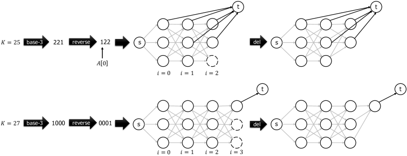
Figure 7: An illustration of the graph construction algorithm for two different values of $K$, using $b=3$. The darker edges are the ones created on stage 6 of Algorithm 1. Note that in the upper construction, the minimum distance between any two path is actually $\rho=3$ and not $\rho=4$ like previously noted. This sometimes holds minor accuracy implications.

Below we show that this construction indeed produces a graph with exactly $K$ paths from source to sink. We start with a technical lemma.

Lemma 3

Let $v\in V\setminus{\left\{t\right\}}$ be a vertex in the $i$th inner slice (where $i\in\left\{0\dots\left\lfloor{\log_{b}{K}}\right\rfloor\right\}$), and let $\mathcal{N}\left(v\right)$ be the number of paths from the source to $v$. Then $\mathcal{N}\left(v\right)=b^{i}$.

Proof: We show this by induction on the slice index $i=0\dots\left\lfloor{\log_{b}{K}}\right\rfloor$. In the base case $i=0$ and $v$ is in the first inner slice (see Figure 7). It has only one incoming edge from the source $s$, hence the statement holds, $\mathcal{N}\left(v\right)=b^{0}=1$.

Next, denote $in\left(v\right)\triangleq\left\{u:\exists\left(u,v\right)\in E\right\}$ and suppose the theorem holds for all slices until the $k$th slice. Let $v$ be a vertex in the $\left(k+1\right)$th slice. Following the graph construction, $v$ has $b$ incoming edges from the vertices in $in\left(v\right)$, all of which are in the $k$th slice. According to the inductive hypothesis, $\forall{u\in in\left(v\right)}:\mathcal{N}\left(u\right)=b^{k}$. Every path from $s$ to $u\in in\left(v\right)$, could be extended to a path from $s$ to $v$ by concatenating the corresponding edge, and so we get that $\mathcal{N}\left(v\right)=\sum_{u\in in\left(v\right)}{\mathcal{N}\left(u\right)}=\sum_{u\in in\left(v\right)}{b^{k}}=b\cdot{b^{k}}=b^{k+1}$.     

Theorem 4

The number of paths from the source to the sink is $K$, i.e. $\mathcal{N}\left(t\right)=K$.

Proof: Let $A\in{\left\{{0\dots b-1}\right\}^{\left\lfloor{\log_{b}{K}}\right\rfloor+1}}$ be the array of the reverse base-$b$ representation of $K$. Using the decomposition of the $b$-ary representation, i.e. $K=\sum_{i=0}^{\left\lfloor{\log_{b}{K}}\right\rfloor}{A\left[i\right]\cdot b^{i}}$, and Lemma 3, we get:

$$\mathcal{N}\left(t\right) =\sum_{v\in in\left(t\right)}{\mathcal{N}\left(v\right)}=\sum_{i=0}^{\left\lfloor{\log_{b}{K}}\right\rfloor}{\left[\sum_{v\in\text{slice}_{i}\cap in\left(t\right)}{\underbrace{\mathcal{N}\left(v\right)}_{=b^{i}}}\right]}=\sum_{i=0}^{\left\lfloor{\log_{b}{K}}\right\rfloor}{\underbrace{\left|{\text{slice}_{i}\cap in\left(t\right)}\right|}_{=A\left[i\right]}\cdot{b^{i}}}$$

$$=\sum_{i=0}^{\left\lfloor{\log_{b}{K}}\right\rfloor}{A\left[i\right]\cdot{b^{i}}}=K~{}.$$

    

C.2 Loss-based decoding generalization

We now show how to adjust the generalization of loss-based decoding for graphs with an arbitrary number of paths $K$, constructed using Algorithm 1.

The idea of the reduction in (2) is that going through an edge $e_{j}$ inflicts the loss of turning its corresponding bit on (i.e. $L\left(1\times f_{j}\left(x\right)\right)$), but also the loss of turning off the bits corresponding to other edges between its slices (i.e. $\sum_{j^{\prime}:e_{j^{\prime}}\in S\left(e_{j}\right)\setminus\left\{e_{j}\right\}}{L\left(\left(-1\right)\times f_{j^{\prime}}\left(x\right)\right)}$), which cannot coappear with $e_{j}$ in the same path (i.e. a codeword).

The only change in the general case is that an edge $e_{j}=\left(u_{j},t\right)$ that is connected to the sink $t$ cannot coappear with any other edge outgoing from a vertex in the same vertical slice as $u_{j}$, or that is reachable from $u_{j}$.

Let $\delta\left(v\right)$ be the shortest distance from the source to $v$ (in terms of number of edges).

We define an updated $S$ function (which is a generalization of the one defined in Section 5), where for every edge ${e_{j}=\left(u_{j},v_{j}\right)\in E}$ we set:

$$S\left(e_{j}\right)=\begin{cases}\left\{\left(u,u^{\prime}\right):\delta\left(u\right)=\delta\left(u_{j}\right)\right\}&v_{j}\neq t\\ \left\{\left(u,u^{\prime}\right):\delta\left(u\right)\geq\delta\left(u_{j}\right)\right\}&v_{j}=t\end{cases}~{},$$ (5)

and the weights are set as in (2) but with the new $S$ function defined in (5),

$$w_{j}\left(x\right)=L\left(1\times f_{j}(x)\right)+\sum_{j{{}^{\prime}}:e_{j^{\prime}}\in S\left(e_{j}\right)\backslash\left\{e_{j}\right\}}L\left((-1)\times f_{j^{\prime}}(x)\right)~{}.$$ (6)

For example, in the following figure we have,

$$S\left(e_{6}\right) =\left\{e_{6},e_{7},e_{8},e_{9}\right\}$$

$$S\left(e_{2}\right) =\left\{e_{2},e_{3},e_{4},e_{5},e_{13}\right\}$$

$$S\left(e_{11}\right) =\left\{e_{10},e_{11}\right\}$$

$$S\left(e_{12}\right) =\left\{e_{12}\right\}$$

$$S\left(e_{13}\right) =\left\{e_{2},\dots,e_{13}\right\}~{}.$$

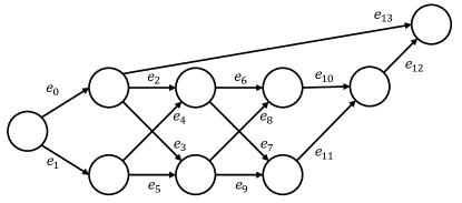
Figure 8: An illustration of a graph with $K=9$ and $b=2$.

Below we show that Theorem 1 is correct for any $K$. Let $P$ be a path on the trellis graph from the source $s$ to the sink $t$. We start will the following lemma.

Lemma 5

Let $e_{q}=\left(u_{q},t\right)$ be the last edge in $P$. For every edge $e_{j}=\left(u_{j},v_{j}\right)\in P\setminus\left\{e_{q}\right\}$ we have $\delta\left(v_{j}\right)=\delta\left(u_{j}\right)+1$.

Proof: Following immediately from the graph construction – other than edges to the sink, there are only edges between adjacent slices (without cycles). Therefore, any vertex $v$ in a vertical slice $i$ (where the leftmost slice containing $s$ is the first one, i.e. $i=0$) holds $\delta\left(v\right)=i$, and every edge $e_{j}=\left(u_{j},v_{j}\right)\in P\setminus\left\{e_{q}\right\}$ holds $\delta\left(v_{j}\right)=\delta\left(u_{j}\right)+1$.     

The next corollaries follow immediately.

Corollary 6

For every two different vertices $u,v\in V\setminus\left\{t\right\}$ along $P$ we have $\delta\left(u\right)\neq\delta\left(v\right)$.

Corollary 7

Let $e_{q}=\left(u_{q},t\right)$ be the last edge in $P$. For every edge $e_{j}=\left(u_{j},v_{j}\right)\in P\setminus\left\{e_{q}\right\}$ we have $\delta\left(u_{j}\right)<\delta\left(u_{q}\right)$.

Clearly, since the graph is directed and acyclic, we get the next lemma.

Lemma 8

Every vertex in $V$ can have at most one incoming edge and one outgoing edge in $P$.

By using Lemma 8, Corollary 6 and Lemma 5 we have the next corollary.

Corollary 9

Set an edge $e_{j}=\left(u_{j},v_{j}\right)$ along the path $P$. Then, $\forall{e_{j{{}^{\prime}}}\in S\left(e_{j}\right)\setminus\left\{e_{j}\right\}}$ we have $e_{j{{}^{\prime}}}\notin P$.

Proof: Let $e_{j{{}^{\prime}}}=\left(u_{j{{}^{\prime}}},v_{j{{}^{\prime}}}\right)$ be any edge in $S\left(e_{j}\right)\setminus\left\{e_{j}\right\}$, and assume $e_{j{{}^{\prime}}}\in P$. We consider two cases:

1. $v_{j}\neq t$:
   By the definition of $S\left(e_{j}\right)$, we get $\delta\left(u_{j{{}^{\prime}}}\right)=\delta\left(u_{j}\right)$. By negating Corollary 6 we get $u_{j{{}^{\prime}}}=u_{j}$. Therefore $e_{j},e_{j{{}^{\prime}}}$ are two edges in $P$ outgoing from the same vertex $u_{j}$, in contradiction to Lemma 8.

2. $v_{j}=t$:
   By definition, $e_{j}\neq e_{j{{}^{\prime}}}$. By Lemma 8 we get that $u_{j}\neq u_{j^{\prime}}$. Also, since $t$ is a sink it has no outgoing edges, thus $u_{j{{}^{\prime}}}\neq t$.

   By the definition of $S\left(e_{j}\right)$, we get $\delta\left(u_{j{{}^{\prime}}}\right)\geq\delta\left(u_{j}\right)$. Since $u_{j{{}^{\prime}}}\neq u_{j}$, we can use Corollary 6 to rule out equivalence and get $\delta\left(u_{j{{}^{\prime}}}\right)>\delta\left(u_{j}\right)$. Following Lemma 5, $u_{j{{}^{\prime}}}$ must appear later than $u_{j}$ in $P$. However, $t$ is the only vertex in $P$ to appear after $u_{j}$ ($t$ is a sink), and since $u_{j{{}^{\prime}}}\neq t$, we get a contradiction.

    

We conclude with the main result of this section, which states that Theorem 1 is correct for any $K$.

Theorem 10

Following the notations of Theorem 1, assume the weights of the edges are calculated as in Eq. (6) with the $S$ function defined in (5). Then, the weight of any path $P_{k}$ corresponding to class $k$ equals to the loss suffered by predicting class $k$, i.e. $w(P_{k})=\sum_{j=1}^{\ell}L\left(M_{k,j}f_{j}(x)\right)$.

Proof:

For any class $k$, we denote the last edge in $P_{k}$ by $e_{q}=\left(u_{q},t\right)$. We have,

$$w\left(P_{k}\right) =\sum_{j:e_{j}\in P_{k}}{w_{j}\left(x\right)}$$

$$=\sum_{j:e_{j}\in P_{k}}\left[L\left(\underbrace{1}_{=M_{k,j}}\times f_{j}\left(x\right)\right)+\sum_{j^{\prime}:e_{j^{\prime}}\in S\left(e_{j}\right)\backslash\left\{e_{j}\right\}}L\left(\underbrace{(-1)}_{\begin{subarray}{c}=M_{k,j{{}^{\prime}}}\\ \text{(Corollary~{}\ref{cor:edgesOfSlice})}\end{subarray}}\times f_{j^{\prime}}(x)\right)\right]$$

$$=\sum_{j:e_{j}\in P_{k}}\left[\sum_{j^{\prime}:e_{j^{\prime}}\in S\left(e_{j}\right)}L\left(M_{k,j{{}^{\prime}}}\times f_{j^{\prime}}(x)\right)\right]$$

$$=\sum_{j:e_{j}\in S(e_{q})}L\left(M_{k,{j}}\times f_{j}(x)\right)+\sum_{j:e_{j}\in P_{k}\setminus\left\{e_{q}\right\}}\left[\sum_{j^{\prime}:e_{j^{\prime}}\in S(e_{j})}L\left(M_{k,{j^{\prime}}}\times f_{j^{\prime}}(x)\right)\right]$$

$$=\sum_{\begin{subarray}{c}j:e_{j}=\left(u_{j},v_{j}\right),\\ \delta\left(u_{j}\right)\geq\delta\left(u_{q}\right)\end{subarray}}L\left(M_{k,j}\times f_{j}(x)\right)+\underbrace{\sum_{j:e_{j}=\left(u_{j},v_{j}\right)\in P_{k}\setminus\left\{e_{q}\right\}}\left[\sum_{\begin{subarray}{c}j{{}^{\prime}}:e_{j{{}^{\prime}}}=\left(u_{j{{}^{\prime}}},v_{j{{}^{\prime}}}\right),\\ \delta\left(u_{j{{}^{\prime}}}\right)=\delta\left(u_{j}\right)\end{subarray}}L\left(M_{k,{j^{\prime}}}\times f_{j^{\prime}}(x)\right)\right]}_{\text{ (Corollary~{}\ref{cor:uqIsMaximal}) ~{}~{}~{}~{}}=\sum_{\begin{subarray}{c}j:e_{j}=\left(u_{j},v_{j}\right),\\ \delta\left(u_{j}\right)<\delta\left(u_{q}\right)\end{subarray}}L\left(M_{k,j}\times f_{j}(x)\right)}$$

$$=\sum_{\begin{subarray}{c}j:e_{j}=\left(u_{j},v_{j}\right),\\ \delta\left(u_{j}\right)\geq\delta\left(u_{q}\right)\end{subarray}}L\left(M_{k,j}\times f_{j}(x)\right)+\sum_{\begin{subarray}{c}j:e_{j}=\left(u_{j},v_{j}\right),\\ \delta\left(u_{j}\right)<\delta\left(u_{q}\right)\end{subarray}}L\left(M_{k,{j}}\times f_{j}(x)\right)$$

$$=\sum_{j:e_{j}\in E}L\left(M_{k,{j}}\times f_{j}(x)\right)$$

$$=\sum_{j=1}^{\ell}L\left(M_{k,j}f_{j}(x)\right)~{}.$$

    

Appendix D Details for complexity analysis in Section 6.1

W-LTLS requires training and storing a binary function or model for every edge. Hence, we first turn to analyze the number of edges.

Lemma 11

The number of vertices in the inner slices is at most $\left({\left\lfloor{\log_{b}{K}}\right\rfloor+1}\right)b$.

Proof: Follows immediately from the construction in Appendix C.1.     

Corollary 12

The number of edges is upper bounded:

$$\left|E\right|\leq\left(b+1\right)\left({\left\lfloor{\log_{b}{K}}\right\rfloor+1}\right)b+b=\mathcal{O}\left(\frac{b^{2}}{\log{b}}\log{K}\right)~{}.$$

Proof: Each vertex in the inner slices can have at most $b+1$ outgoing edges. We use Lemma 11 and count also the $b$ edges outgoing from the source.     

For most linear classifiers (with $d$ parameters each) we get a total model size complexity of $\mathcal{O}\left(d\frac{b^{2}}{\log{b}}\log{K}\right)$.

Inference consists of four steps:

1. Computing the value (margin) of all binary functions on the input $x$. This requires $\mathcal{O}\left(d\left|E\right|\right)=\mathcal{O}\left(d\frac{b^{2}}{\log{b}}\log{K}\right)$ time.

2. Computing the edge weights $\left\{w_{i}\left(x\right)\right\}_{i=1}^{\ell}$ as explained in Section 5. This can be performed in $\mathcal{O}\left(\left|V\right|+\left|E\right|\right)=\mathcal{O}\left(\frac{b^{2}}{\log{b}}\log{K}\right)$ time using a simple dynamic programming algorithm (e.g. implementing back recursion).

3. Finding the shortest path in the trellis graph with respect to $\left\{w_{i}\left(x\right)\right\}_{i=1}^{\ell}$ using the Viterbi algorithm in $\mathcal{O}\left(\left|V\right|+\left|E\right|\right)=\mathcal{O}\left(\frac{b^{2}}{\log{b}}\log{K}\right)$ time.

4. Decoding the shortest path to a class. As explained in Section 4.1, the inference requires a mapping function from path to code. Using data structures such as a binary tree, this can be performed in a $\mathcal{O}\left(\left|E\right|\right)=\mathcal{O}\left(\frac{b^{2}}{\log{b}}\log{K}\right)$ time complexity.

We get that the total inference time complexity is $\mathcal{O}\left(d\left|E\right|\right)=\mathcal{O}\left(d\frac{b^{2}}{\log{b}}\log{K}\right)$.

Appendix E Experiments appendix

E.1 Datasets used in experiments

Dataset	Classes	Features	Train Samples
	$K$	$d$	$m$
sector	105	55,197	7,793
aloi_bin	1,000	636,911	90,000
imageNet	1,000	1,000	1,125,264
Dmoz	11,947	833,484	335,068
LSHTC1	12,294	1,199,856	83,805

Table 1: Datasets used in the experiments.

E.2 Average binary training loss

We validate our hypothesis that wider graphs lead to easier binary problems. In the first row of Figure 9 we plot the average binary training loss $\varepsilon$ as a function of model size. The average is both over the induced binary subproblems and over the five runs.

In all datasets we observe a decrease of the average error as the slice width $b$ grows. The decrease is sharp for low values of $b$ and then practically almost converges (to zero). These plots validate our claim – as the subproblems become more unbalanced they also become easier.

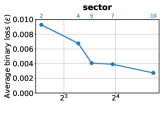
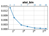
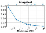
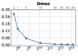
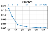
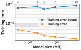
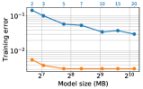
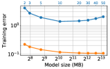
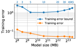
Figure 9: First row: Average binary loss ($\varepsilon$) vs Model size. Second row: Multiclass training error and multiclass training error bound (on a logarithmic scale) vs Model size. The secondary x-axes (top axes, blue) indicate the slice widths (b) used for the W-LTLS trellis graphs.

E.3 Multiclass training error

In the second row of Figure 9 we plot the multiclass training error (when using loss-based decoding defined in (1) with the squared hinge loss) and its bound (3) for different model sizes (MBytes).

For the bound, we set the minimum distance $\rho=4$ as explained in Section 6, and $L_{SH}(0)=1$. The average binary loss $\varepsilon$ was computed as in (4).

For all datasets, the multiclass training error follows qualitatively its bound. For the two larger datasets, shown in the two right panels, both the error and its bound decrease to some point, and then start to increase. This can be explained as follows: at some point, the increase in the slice widths (and $\ell$ and the model size), stops to significantly decrease $\epsilon$ (see first row of Figure 9), such that the term $\ell\times\varepsilon$ appears in the training error bound (3) overall starts increasing (recall that the denominator $\rho\times L\left(0\right)$ is constant). By comparing these plots to the multiclass test accuracy plots in Figure 5, we observe that at the same point where the training error and its bound start to increase, the test accuracy does not increase significantly anymore. For example, for LSHTC1 and Dmoz datasets, the training error bounds start to increase at around model size of $2^{12}$ , and at the same time the test accuracy stops increasing significantly. This suggests that model size of $2^{12}$ is a good point in terms of accuracy/model size tradeoff.

E.4 Average predictions margin

As discussed in Section 7.1, the following Figure 10 shows that for larger values of $b$, the predictions margin increases.

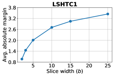
Figure 10: The average absolute margin, i.e. $\frac{1}{m\ell}\sum_{i=1}^{m}{\sum_{j=1}^{\ell}{\left|f_{j}\left(x_{i}\right)\right|}}$, vs the slice width $b$.

E.5 Experimental results of the multiclass test accuracy experiments

Following are the results of Section 7.2 organized in a tabular form – the model sizes and prediction times of the tested algorithms and their test accuracy. The results of W-LTLS are averaged on five runs.

Dataset	Algorithm		Model	Prediction	Test
			size (Bytes)	time (sec)	accuracy (%)
sector	LTLS		5.9 MB	0.14	88.45
	W-LTLS	$b=2$	5.9 MB	0.14	91.63
		$b=4$	9.7 MB	0.16	93.92
		$b=5$	11.6 MB	0.16	94.32
		$b=7$	15.4 MB	0.18	94.86
		$b=10$	26.5 MB	0.23	94.88
	LOMTree		17.0 MB	0.16	82.10
	FastXML		8.9 MB	0.32	86.26
	OVR		41.3 MB	-	94.79
aloi.bin	LTLS		102.1 MB	1.0	82.24
	W-LTLS	$b=2$	102.1 MB	1.4	85.03
		$b=3$	133.6 MB	1.5	89.39
		$b=5$	216.2 MB	1.7	92.49
		$b=7$	328.0 MB	2.1	93.70
		$b=10$	537.0 MB	2.7	94.92
		$b=15$	777.5 MB	3.5	94.93
		$b=20$	1.1 GB	5.0	95.16
	LOMTree		106.0 MB	1.6	89.47
	FastXML		522.0 MB	5.3	95.38
	OVR		2.4 GB	-	95.90
imageNet	LTLS		0.16 MB	15.0	0.75
	W-LTLS	$b=2$	0.16 MB	21.4	0.42
		$b=5$	0.34 MB	26.3	1.59
		$b=10$	0.84 MB	40.3	4.36
		$b=15$	1.2 MB	52.6	4.08
		$b=20$	1.8 MB	76.2	7.01
		$b=30$	3.7 MB	194.2	12.60
	LOMTree		35.0 MB	37.7	5.37
	FastXML		1.6 GB	172.3	6.84
	OVR		3.8 MB	-	15.60
Dmoz	LTLS		193.9 MB	5.2	23.04
	W-LTLS	$b=2$	193.9 MB	7.5	25.76
		$b=3$	248.0 MB	8.1	29.56
		$b=5$	429.2 MB	9.8	33.92
		$b=10$	1.1 GB	16.6	37.44
		$b=20$	2.8 GB	41.4	38.43
		$b=30$	4.3 GB	73.6	38.89
		$b=40$	6.3 GB	164.5	38.81
		$b=50$	9.0 GB	332.3	38.89
	LOMTree		1.8 GB	28.0	21.27
	FastXML		1.2 GB	60.7	38.58
	OVR		38.0 GB	-	35.50
LSHTC1	LTLS		256.3 MB	0.65	9.50
	W-LTLS	$b=2$	256.3 MB	1.1	10.56
		$b=3$	361.6 MB	1.1	13.72
		$b=5$	631.6 MB	1.3	16.58
		$b=10$	1.5 GB	2.2	20.44
		$b=20$	4.0 GB	5.1	21.76
		$b=30$	6.3 GB	9.9	22.08
		$b=40$	9.0 GB	20.4	22.30
		$b=45$	10.8 GB	29.3	22.47
	LOMTree		744.0 MB	6.8	10.56
	FastXML		366.6 MB	10.7	21.66
	OVR		56.3 GB	-	21.90

E.6 Experimental results of the sparsity experiments

In the following Figure 11 we show that wider graphs induce models which use less features, even before pruning.

This may help understand the results in Section 7.3, where we show that the larger slice widths allow pruning more weights without accuracy degradation.

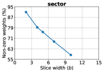
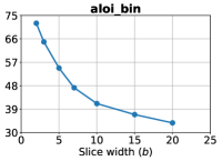
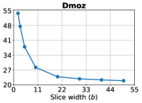
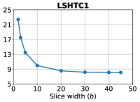
Figure 11: Percentage of non-zero weights at end of training (before pruning) vs the slice width $b$.

In the following Table 2, the results of Section 7.3 organized in a tabular form.

Dataset	Algorithm			Model	Test
				size (Bytes)	accuracy (%)
sector	Sparse W-LTLS	$b=2$	${\lambda}=0.324$	1.4 MB	90.66
		$b=4$	${\lambda}=0.303$	1.0 MB	93.42
		$b=5$	${\lambda}=0.327$	1.1 MB	93.86
		$b=7$	${\lambda}=0.341$	1.0 MB	94.11
		$b=10$	${\lambda}=0.358$	0.74 MB	94.82
	FastXML	$T=25$		4.5 MB	86.26
		$T=50$		8.9 MB	86.26
		$T=75$		13.4 MB	86.78
		$T=100$		17.9 MB	86.58
		$T=150$		26.8 MB	86.57
		$T=200$		35.8 MB	87.20
aloi.bin	Sparse W-LTLS	$b=2$	${\lambda}=0.015$	37.3 MB	84.09
		$b=3$	${\lambda}=0.015$	32.7 MB	88.59
		$b=5$	${\lambda}=0.017$	25.4 MB	91.74
		$b=7$	${\lambda}=0.016$	25.9 MB	92.89
		$b=10$	${\lambda}=0.013$	30.3 MB	94.48
		$b=15$	${\lambda}=0.014$	31.2 MB	94.27
		$b=20$	${\lambda}=0.016$	25.4 MB	94.55
	FastXML	$T=5$		52.1 MB	92.67
		$T=10$		104.2 MB	94.12
		$T=25$		260.9 MB	95.19
		$T=50$		522.0 MB	95.38
		$T=100$		1.0 GB	95.66
	DiSMEC			10.7 MB	96.28
	PD-Sparse			12.7 MB	96.20
	PPDSparse			9.3 MB	96.38
Dmoz	Sparse W-LTLS	$b=2$	${\lambda}=0.347$	43.2 MB	24.64
		$b=3$	${\lambda}=0.325$	56.1 MB	28.63
		$b=5$	${\lambda}=0.314$	69.3 MB	33.04
		$b=10$	${\lambda}=0.323$	93.7 MB	36.75
		$b=20$	${\lambda}=0.345$	126.3 MB	37.72
		$b=30$	${\lambda}=0.385$	145.6 MB	38.08
		$b=40$	${\lambda}=0.374$	193.1 MB	38.08
		$b=50$	${\lambda}=0.323$	324.3 MB	38.16
	FastXML	$T=1$		24.5 MB	27.09
		$T=2$		49.2 MB	31.17
		$T=5$		123.0 MB	35.84
		$T=10$		246.5 MB	37.47
		$T=50$		1.2 GB	38.58
		$T=300$		7.4 GB	38.63
	DiSMEC			259.3 MB	39.38
	PD-Sparse			453.3 MB	39.91
	PPDSparse			526.7 MB	39.32
LSHTC1	Sparse W-LTLS	$b=2$	${\lambda}=0.288$	24.7 MB	9.48
		$b=3$	${\lambda}=0.237$	27.6 MB	12.66
		$b=5$	${\lambda}=0.271$	31.5 MB	15.60
		$b=10$	${\lambda}=0.226$	46.3 MB	19.78
		$b=20$	${\lambda}=0.207$	85.0 MB	21.13
		$b=30$	${\lambda}=0.192$	130.5 MB	21.56
		$b=40$	${\lambda}=0.183$	184.7 MB	21.81
		$b=45$	${\lambda}=0.246$	152.1 MB	21.88
	FastXML	$T=1$		7.3 MB	12.50
		$T=5$		36.6 MB	17.98
		$T=10$		73.3 MB	19.36
		$T=50$		366.6 MB	21.66
		$T=150$		1.1 GB	21.94
		$T=300$		2.2 GB	22.04
		$T=1200$		8.8 GB	21.92
	DiSMEC			94.7 MB	22.74
	PD-Sparse			58.7 MB	22.46
	PPDSparse			254.0 MB	22.70

Table 2: Simulation results for the sparse models.

References

- [1] Erin L. Allwein, Robert E. Schapire, and Yoram Singer. Reducing multiclass to binary: A unifying approach for margin classifiers. Journal of Machine Learning Research, 1:113–141, 2000.
- [2] Rohit Babbar and Bernhard Schölkopf. Dismec: Distributed sparse machines for extreme multi-label classification. In Proceedings of the Tenth ACM International Conference on Web Search and Data Mining, WSDM ’17, pages 721–729, New York, NY, USA, 2017. ACM.
- [3] Samy Bengio, Jason Weston, and David Grangier. Label embedding trees for large multi-class tasks. Advances in Neural Information Processing Systems, 23(1):163–171, 2010.
- [4] Alina Beygelzimer, John Langford, Yuri Lifshits, Gregory Sorkin, and Alex Strehl. Conditional probability tree estimation analysis and algorithms. In Proceedings of the Twenty-Fifth Conference on Uncertainty in Artificial Intelligence, UAI ’09, pages 51–58, Arlington, Virginia, United States, 2009. AUAI Press.
- [5] Kush Bhatia, Himanshu Jain, Purushottam Kar, Manik Varma, and Prateek Jain. Sparse local embeddings for extreme multi-label classification. In Advances in Neural Information Processing Systems 28: Annual Conference on Neural Information Processing Systems 2015, December 7-12, 2015, Montreal, Quebec, Canada, pages 730–738, 2015.
- [6] Erin J. Bredensteiner and Kristin P. Bennett. Multicategory classification by support vector machines. Computational Optimizations and Applications, 12:53–79, 1999.
- [7] Anna Choromanska and John Langford. Logarithmic time online multiclass prediction. In Proceedings of the 28th International Conference on Neural Information Processing Systems - Volume 1, NIPS’15, pages 55–63, Cambridge, MA, USA, 2015. MIT Press.
- [8] Moustapha Cisse, Thierry Artieres, and Patrick Gallinari. Learning compact class codes for fast inference in large multi class classification. Lecture Notes in Computer Science (including subseries Lecture Notes in Artificial Intelligence and Lecture Notes in Bioinformatics), 7523 LNAI(PART 1):506–520, 2012.
- [9] Corinna Cortes and Vladimir Vapnik. Support-vector networks. Machine learning, 20(3):273–297, 1995.
- [10] Koby Crammer, Alex Kulesza, and Mark Dredze. Adaptive regularization of weight vectors. In Advances in Neural Information Processing Systems 22, pages 414–422. Curran Associates, Inc., 2009.
- [11] Koby Crammer and Yoram Singer. On the algorithmic implementation of multiclass kernel-based vector machines. Jornal of Machine Learning Research, 2:265–292, 2001.
- [12] Hal Daumé, III, Nikos Karampatziakis, John Langford, and Paul Mineiro. Logarithmic time one-against-some. In Proceedings of the 34th International Conference on Machine Learning, volume 70 of Proceedings of Machine Learning Research, pages 923–932, International Convention Centre, Sydney, Australia, 06–11 Aug 2017. PMLR.
- [13] Krzysztof Dembczyński, Wojciech Kotłowski, Willem Waegeman, Róbert Busa-Fekete, and Eyke Hüllermeier. Consistency of probabilistic classifier trees. In Machine Learning and Knowledge Discovery in Databases, pages 511–526, Cham, 2016. Springer International Publishing.
- [14] Thomas G. Dietterich and Ghulum Bakiri. Solving Multiclass Learning Problems via Error-Correcting Output Codes. Jouranal of Artifical Intelligence Research, 2:263–286, 1995.
- [15] Ian En-Hsu Yen, Xiangru Huang, Pradeep Ravikumar, Kai Zhong, and Inderjit S. Dhillon. PD-Sparse : A Primal and Dual Sparse Approach to Extreme Multiclass and Multilabel Classification. Proceedings of The 33rd International Conference on Machine Learning, 48:3069–3077, 2016.
- [16] Sergio Escalera, Oriol Pujol, and Petia Radeva. Loss-Weighted Decoding for Error-Correcting Output Coding. Visapp (2), pages 117–122, 2008.
- [17] Johannes Fürnkranz. Round robin classification. Jornal of Machine Learning Research, 2:721–747, March 2002.
- [18] Himanshu Jain, Yashoteja Prabhu, and Manik Varma. Extreme multi-label loss functions for recommendation, tagging, ranking & other missing label applications. In Proceedings of the 22Nd ACM SIGKDD International Conference on Knowledge Discovery and Data Mining, KDD ’16, pages 935–944, New York, NY, USA, 2016. ACM.
- [19] Kalina Jasinska and Nikos Karampatziakis. Log-time and log-space extreme classification. arXiv preprint arXiv:1611.01964, 2016.
- [20] Yacine Jernite, Anna Choromanska, and David Sontag. Simultaneous learning of trees and representations for extreme classification and density estimation. In Proceedings of the 34th International Conference on Machine Learning, ICML 2017, Sydney, NSW, Australia, 6-11 August 2017, pages 1665–1674, 2017.
- [21] Ashraf M. Kibriya and Eibe Frank. An Empirical Comparison of Exact Nearest Neighbour Algorithms. Knowledge Discovery in Databases: PKDD 2007, pages 140–151, 2007.
- [22] Shengren Li and Nina Amenta. Brute-force k-nearest neighbors search on the GPU. In Similarity Search and Applications - 8th International Conference, SISAP 2015, Glasgow, UK, October 12-14, 2015, Proceedings, pages 259–270, 2015.
- [23] Shu Lin and Daniel J. Costello. Error Control Coding, Second Edition. Prentice-Hall, Inc., Upper Saddle River, NJ, USA, 2004.
- [24] Mingxia Liu, Daoqiang Zhang, Songcan Chen, and Hui Xue. Joint binary classifier learning for ecoc-based multi-class classification. IEEE Transactions on Pattern Analysis and Machine Intelligence, 38(11):2335–2341, Nov. 2016.
- [25] Chris Mesterharm. A multi-class linear learning algorithm related to winnow. In Advances in Neural Information Processing Systems 13, 1999.
- [26] Frederic Morin and Yoshua Bengio. Hierarchical probabilistic neural network language model. In Proceedings of the Tenth International Workshop on Artificial Intelligence and Statistics, pages 246–252. Society for Artificial Intelligence and Statistics, 2005.
- [27] Mohammad Norouzi, Ali Punjani, and David J. Fleet. Fast exact search in hamming space with multi-index hashing. IEEE Transactions on Pattern Analysis and Machine Intelligence, 36(6):1107–1119, 2014.
- [28] Yashoteja Prabhu, Anil Kag, Shrutendra Harsola, Rahul Agrawal, and Manik Varma. Parabel: Partitioned label trees for extreme classification with application to dynamic search advertising. In Proceedings of the 2018 World Wide Web Conference, WWW ’18, 2018.
- [29] Yashoteja Prabhu and Manik Varma. Fastxml: A fast, accurate and stable tree-classifier for extreme multi-label learning. In Proceedings of the 20th ACM SIGKDD International Conference on Knowledge Discovery and Data Mining, KDD ’14, pages 263–272, 2014.
- [30] Robert E. Schapire. Explaining adaboost. In Empirical Inference - Festschrift in Honor of Vladimir N. Vapnik, pages 37–52, 2013.
- [31] Yukihiro Tagami. Annexml: Approximate nearest neighbor search for extreme multi-label classification. In Proceedings of the 23rd ACM SIGKDD International Conference on Knowledge Discovery and Data Mining, KDD ’17, pages 455–464, New York, NY, USA, 2017. ACM.
- [32] Andrew J. Viterbi. Error bounds for convolutional codes and an asymptotically optimum decoding algorithm. IEEE Trans. Information Theory, 13(2):260–269, 1967.
- [33] Jason Weston, Samy Bengio, and Nicolas Usunier. WSABIE: Scaling up to large vocabulary image annotation. IJCAI International Joint Conference on Artificial Intelligence, pages 2764–2770, 2011.
- [34] Jason Weston and Chris Watkins. Support vector machines for multi-class pattern recognition. In Esann, volume 99, pages 219–224, 1999.
- [35] Ian E.H. Yen, Xiangru Huang, Wei Dai, Pradeep Ravikumar, Inderjit Dhillon, and Eric Xing. Ppdsparse: A parallel primal-dual sparse method for extreme classification. In Proceedings of the 23rd ACM SIGKDD International Conference on Knowledge Discovery and Data Mining, KDD ’17, pages 545–553, New York, NY, USA, 2017. ACM.
- [36] Hsiang-Fu Yu, Prateek Jain, Purushottam Kar, and Inderjit Dhillon. Large-scale multi-label learning with missing labels. In International conference on machine learning, pages 593–601, 2014.
- [37] Bin Zhao and Eric P. Xing. Sparse Output Coding for Scalable Visual Recognition. International Journal of Computer Vision, 119(1):60–75, 2013.