Abstract

It has been recently shown that tachyonic chameleon model of dark energy in which tachyon scalar field non-minimally coupled to the matter admits stable scaling attractor solution that could give rise to the late-time accelerated expansion of the universe and hence alleviate the coincidence problem. In the present work, we use data from Type Ia supernova (SN Ia) and Baryon Acoustic Oscillations to place constraints on the model parameters. In our analysis we consider in general exponential and non-exponential forms for the non-minimal coupling function and tachyonic potential and show that the scenario is compatible with observations.

1 Introduction

Recent cosmological observations such as Type Ia supernova (SN Ia)(Perlmutter et al., 1999; Riess et al., 1998), cosmic microwave background (CMB) radiation (Ade et al., 2016; Ade et al., 2014; Komatsu et al., 2011; Hinshaw et al., 2013), large scale structure (Tegmark et al., 2004; Seljak et al., 2005), Baryon Acoustic Oscillations (BAO) (Eisenstein et al., 2005) and weak lensing (Jain & Taylor, 2003) indicate that the expansion of the current universe is accelerating.
Though the $\Lambda CDM$ cosmology in which $\Lambda$ is the cosmological constant can successfully reproduce the late time cosmic acceleration, it suffers from some serious issues such as the fine tuning and cosmological coincidence problems (Ellis & Madsen, 1995; Starobinsky, 1998). So, two alternative approaches have been proposed to explain the current behaviour of the universe. The first is to consider the modification of gravity on the large scale (see (Nojiri & Odintsov, 2007) for review and reference there in) and the second is introducing dark energy sector in the content of the universe (see (Copeland, Sami & Tsujikawa, 2006) for review). It is worthwhile to notice that in the second approach one can also include a non-minimal coupling between dark energy and gravity to construct scalar-tensor theories (see for example ( Nojiri & Odintsov, 2005)).
Besides scalar-tensor theories in which scalar field non-minimally couples to the Ricci scalar or other geometric terms, recently another form of a non-minimally coupled scalar field where the scalar field is coupled to the matter has been widely studied in the literature ( Das & Banerjee, 2008; Farajollahi et al., 2012; Bisabr, 2012). This type of scalar field is known as a chameleon field and thought it is heavy in the laboratory environment, on cosmological scale where the matter density is small, the chameleon is light enough to play the role of dark energy.
A chameleon scalar field has many remarkable cosmological features as they pointed out by many authors. For instance, when it couples to an electromagnetic field (Khoury & Weltman, 2011) [19] in addition to the fluid then the fine tuning of the initial condition on the chameleon may be resolved (Mota & Schelpe, 2012). Chameleon field can also successfully explain a smooth transition from a deceleration to an acceleration epoch for our universe (Banerjee & Das, 2010). The scalar field that plays the role of chameleon could be a Brans-Dicke scalar field with interesting cosmological consequences such as explaining the current accelerated expansion of the universe (Banerjee & Das, 2010; Khoury & Weltman 2004; Das, Corasaniti & Khoury, 2006). Koury in (Khoury, 2013) has summarized some important features of the chameleon field theories. Moreover, phase-space analysis of chameleon scalar field where a quintessence field acts as a chameleon has been investigate in (Roy & Banerjee, 2015). We have also studied the dynamics of chameleon model where tachyon field plays the role of chameleon (Banijamali & Solbi, 2017). We have utilized the dynamical system tools to obtain the critical points of such theory and showed its interesting cosmological behaviour.
In the present work we apply combined datasets of Type Ia Supernova (SN Ia) and Baryon Acoustic Oscillations to test the tachyonic chameleon model and constrain its parameters. We use $\chi^{2}$ minimization technique to find the best fit values of the model parameters and to plot the likelihood contours for them.
The paper is organized as follows: In the next section we have presented the tachyonic chameleon model and derived the basic equations along with the definitions of different cosmological parameters relevant for our study. In section 3 we have briefly discussed our methodology to use data from SN Ia and BAO observations. In section 4 we have used the observational data to plot likelihood contours of the model for different categories of scalar potential and coupling function. Section 5 is devoted to our conclusion.

2 Basic equations

Tachyonic chameleon model of dark energy in the framework of general relativity can be described by the following action

$$S=\int d^{4}x\sqrt{-g}\Big{[}\frac{R}{16\pi G}-V(\phi)\sqrt{1-\partial_{\mu}\phi\partial^{\nu}\phi}+f(\phi)\mathcal{L}_{m}\Big{]},$$ (1)

where $g$ is the determinant of the metric tensor $g_{\mu\nu}$, $R$ is the Ricci scalar and $G$ is the bare gravitational constant. $f(\phi)$ is the coupling function between scalar field and the matter. $\mathcal{L}_{m}$ is the matter Lagrangian and $V(\phi)$ is also the tachyon potential.
Variation of action (1) with respect to the metric $g_{\mu\nu}$ leads to the gravitational field equations. These equations in FRW background with the metric

$$ds^{2}=dt^{2}-a^{2}(dr^{2}+r^{2}d\theta^{2}+r^{2}sin^{2}\theta d\phi^{2}),$$ (2)

take the following forms:

$$3H^{2}=\rho_{m}f+\frac{V(\phi)}{\sqrt{1-\dot{\phi}^{2}}},$$ (3)

$$2\dot{H}+3H^{2}=-\gamma\rho_{m}f+V(\phi)\sqrt{1-\dot{\phi}^{2}},$$ (4)

where $\rho_{m}$ and $p_{m}$ are the matter energy density and pressure respectively. In fact equations (3) and (4) are the Friedmann equations for our model. Note also that $p_{m}=\gamma\rho_{m}$ is assumed in deriving these equations.
On the other hand, variation of (1) with respect to thescalar field in FRW background yields to

$$\ddot{\phi}+(1-\dot{\phi}^{2})(3H\dot{\phi}+\frac{V^{\prime}}{V})=(1-3\gamma)(1-\dot{\phi}^{2})^{\frac{3}{2}}\frac{\rho_{m}f^{\prime}}{V},$$ (5)

where the tachyon field is assumed to be homogeneous and a prime stands for derivative with respect to the $\Phi$.
In addition, the continuity equation reads,

$$(\rho_{m}f)\dot{}+3H(1+\gamma)\rho_{m}f=-(1-3\gamma)\rho_{m}\dot{f}.$$ (6)

Now, we mention that equation (6) has a solution as follows:

$$\rho_{m}=\rho_{0}a^{-3(1+\gamma)}f^{-(2-3\gamma)}$$ (7)

where $\rho_{0}$ is an integration constant. This shows the evolution of the matter density strongly depends on the coupling function $f$. When $f=1$, this solution reduces to the standard evolution law for the matter energy density.
Furthermore, one can define the effective equation of state as

$$\omega_{eff}\equiv\frac{p_{eff}}{\rho_{eff}},$$ (8)

where $p_{eff}$ and $\rho_{eff}$ can be obtained from (3) and (4) as follows:

$$p_{eff}=\gamma\rho_{m}f-V(\phi)\sqrt{1-\dot{\phi}^{2}},$$ (9)

$$\rho_{eff}=\rho_{m}f+\frac{V(\phi)}{\sqrt{1-\dot{\phi}^{2}}}.$$ (10)

Before closing this section notice that, tachyonic chameleon dark energy model exhibits some interesting cosmological implication from dynamical system point of view. Depending on the form of coupling function $f(\phi)$ and potential $V(\phi)$ such a model provides a solution to coincidence problem and explains the current phase of accelerated expansion of the universe ( Banijamali & Solbi 2017). Therefore, investigating this scenario using observational cosmology and constraining the model parameters according to the latest data is not only interesting but also necessary. This study will be done in the next sections.

3 Observational constraints on the model parameters

In this section, we will fit the model parameters with recent observational data from Type Ia Supernova (SN Ia) and Baryon Acoustic Oscillations (BAO) observations. Although a well-known analysis method is used in the literature, we briefly explain the method for the elaboration of the observational data.
The total $\chi^{2}$ for combined data analysis is given by:

$$\chi^{2}=\chi_{\mathrm{SN}}^{2}+\chi_{\mathrm{BAO}}^{2},$$ (11)

where each $\chi^{2}$ will be evaluated individually. We mention that in our fitting method we use the simple $\chi^{2}$ method (Perivolaropoulos 2013) , rather than the Markov-chain Monte Carlo (MCMC) procedure such as CosmoMC (Lewis & Bridle 2002).
Now we are going to explain the way by which one can calculate each $\chi^{2}$ (Yang et al 2010; Li et al 2010) .

3.1 Type Ia Supernova (SN Ia)

First, we have used the latest observational dataset of SN Ia which give the information on the luminosity distance $D_{L}$ as a function of the red shift $z$.
The Hubble-free luminosity distance for the flat universe is defined as

$$D_{L}(z)=\left(1+z\right)\int_{0}^{z}\frac{dz^{\prime}}{E(z^{\prime})}\,,$$

where $E(z)\equiv H(z)/H_{0}$, with

$$\frac{H(z)}{H_{0}}=\sqrt{\Omega_{\mathrm{m}}^{(0)}\left(1+z\right)^{3}+\Omega_{\mathrm{r}}^{(0)}\left(1+z\right)^{4}+\Omega_{\mathrm{DE}}^{(0)}\left(1+z\right)^{3\left(1+w_{\mathrm{DE}}\right)}}\,.$$

Here, $\Omega_{\mathrm{r}}$ is the radiation density parameter and $\Omega_{\mathrm{r}}^{(0)}=\Omega_{\gamma}^{(0)}\left(1+0.2271N_{\mathrm{eff}}\right)$, where $\Omega_{\gamma}^{(0)}$ is the present fractional photon energy density and $N_{\mathrm{eff}}=3.04$ is the effective number of neutrino species (Komatsu et al 2011).
The theoretical distance modulus $\mu_{\mathrm{th}}$ is defined by

$$\mu_{\mathrm{th}}(z_{i})\equiv 5\log_{10}D_{L}(z_{i})+\mu_{0}\,,$$

where $\mu_{0}\equiv 42.38-5\log_{10}h$, with $h\equiv H_{0}/100/[\mathrm{km}\,\mathrm{sec}^{-1}\,\mathrm{Mpc}^{-1}]$ (Komatsu et al 2011).
For SN Ia dataset, $\chi^{2}$ function is given by

$$\chi_{\mathrm{SN}}^{2}=\sum_{i}\frac{\left[\mu_{\mathrm{obs}}(z_{i})-\mu_{\mathrm{th}}(z_{i})\right]^{2}}{\sigma_{i}^{2}}\,,$$ (12)

where $\mu_{\mathrm{obs}}$ is the observed value of the distance modulus. $\chi_{\mathrm{SN}}^{2}$ in the above equation can by expanded as ( Perivolaropoulos 2005)

$$\chi_{\mathrm{SN}}^{2}=A-2\mu_{0}B+\mu_{0}^{2}C\,,$$

where

$$A=\sum_{i}\frac{\left[\mu_{\mathrm{obs}}(z_{i})-\mu_{\mathrm{th}}(z_{i};\mu_{0}=0)\right]^{2}}{\sigma_{i}^{2}}\,,\quad$$

$$B=\sum_{i}\frac{\mu_{\mathrm{obs}}(z_{i})-\mu_{\mathrm{th}}(z_{i};\mu_{0}=0)}{\sigma_{i}^{2}}\,,\quad$$

$$C=\sum_{i}\frac{1}{\sigma_{i}^{2}}\,.$$

Note that $\mu_{obs}$ and $\mu_{th}$ represent the observed and theoretical distance modulus respectively. $\sigma_{i}$ is also the uncertainly in the distance modulus.
Finally, minimizing $\chi_{\mathrm{SN}}^{2}$ with respect to $\mu_{0}$ leads to

$$\tilde{\chi}_{\mathrm{SN}}^{2}=A-\frac{B^{2}}{C}\,.$$ (13)

We use (13) for minimization of $\chi^{2}$ for 580 recent data points of SN Ia (Suzuki et al. 2011).

3.2 Baryon Acoustic Oscillations (BAO)

We have also used BAO dataset to constrain our model parameters. The distance ratio $d_{z}\equiv r_{s}(z_{\mathrm{d}})/D_{V}(z)$ is measured by BAO observations. Here $D_{V}$ is the volume-averaged distance, $r_{s}$ is the comoving sound horizon and $z_{\mathrm{d}}$ is the redshift at the drag epoch (Percival et al. 2009).
Distance $D_{V}(z)$ is defined as (Eisenstein 2005)

$$D_{V}(z)\equiv\left[\left(1+z\right)^{2}D_{A}^{2}(z)\frac{z}{H(z)}\right]^{1/3}\,,$$

where $D_{A}(z)$ is the proper angular diameter distance for the flat universe.
In our analysis we use the 6dF, the SDSS and WiggleZ BAO data points which are represented in Table 1. The WiggleZ collaboration (Blake et al. 2011) has measured the baryon acoustic scale at three different redshifts, while SDSS and 6DFGS surveys provide data at lower redshift (Percival 2010).

	6dF	SDSS		WiggleZ
$z$	0.106	0.2	0.35	0.44	0.6	0.73
$d_{z}$	0.336	0.1905	0.1097	0.0916	0.0726	0.0592
$\Delta d_{z}$	0.015	0.0061	0.0036	0.0071	0.0034	0.0032

Table 1: The BAO data used in our analysis.

In addition, $C_{\mathrm{BAO}}^{-1}$ was obtained from the covariance data (Blake et al. 2011) in terms of $d_{z}$ as follows:

$$C_{\mathrm{BAO}}^{-1}=\left(\begin{array}[]{cccccc}4444&0&0&0&0&0\\ 0&30318&-17312&0&0&0\\ 0&-17312&87046&0&0&0\\ 0&0&0&23857&-22747&10586\\ 0&0&0&-22747&128729&-59907\\ 0&0&0&10586&-59907&125536\end{array}\right)\,.$$

At last, $\chi^{2}$ for the BAO data is expressed as

$$\chi_{\mathrm{BAO}}^{2}=\left(x_{i,\mathrm{BAO}}^{\mathrm{th}}-x_{i,\mathrm{BAO}}^{\mathrm{obs}}\right)\left(C_{\mathrm{BAO}}^{-1}\right)_{ij}\left(x_{j,\mathrm{BAO}}^{\mathrm{th}}-x_{j,\mathrm{BAO}}^{\mathrm{obs}}\right),$$

where the indices $i,j$ are in growing order in $z$, as in Table 1. In the next section we use the above two sets of data to examine our model.

4 Observational constraints on the model parameters

Two important functions in the model (1) are the chameleon field potential $V(\phi)$ and coupling function $f(\phi)$. We perform our analysis based on this fact that whether these functions are exponential (power-law) or not. Thus we have four categories given by the following subsections:

4.1 Exponential $f(\phi)$ and power-law $V(\phi)$

In the first case we consider an exponential coupling function and a power-law potential as follows’

$$f(\phi) =f_{0}e^{\alpha\phi},$$

$$V(\phi) =V_{0}\phi^{\beta}.$$ (14)

We are interested in constraining model parameters $\alpha$ and $\beta$ together with the present values of the density parameters using the $\chi^{2}$-method for recent observational data. Thus we plot the likelihood contours for these physically important parameters and obtain the best fit values. We produce the likelihood contours for $1\sigma$ , $2\sigma$ and $3\sigma$ confidence levels.

Data	$\chi_{min}^{2}$	$\Omega_{m_{0}}$	$\alpha$	$\beta$
SN Ia +	584.08	0.29	-1.53	1.96
BAO

Table 2: The value of $\chi_{min}^{2}$ and the best fit values of model parameters $\Omega_{m_{0}}$, $\alpha$ and $\beta$ for the first case.

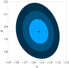
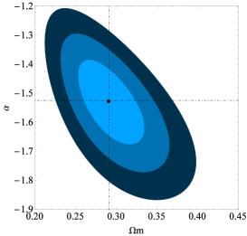
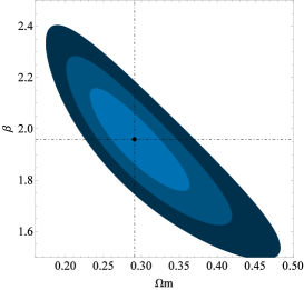
In Figure 1 the $1\sigma$, $2\sigma$ and $3\sigma$ confidence level contours for $\alpha-\beta$ (a), $\alpha-\Omega_{m_{0}}$ (b) and $\beta-\Omega_{m_{0}}$ (c) are plotted for SN Ia +BAO datasets. For simplicity reasons we set $f_{0}=V_{0}=1$. As one can see in this figure this model is in agreement with observations. The best-fit values of $\alpha$, $\beta$ and $\Omega_{m_{0}}$ in addition to $\chi^{2}_{min}$ (the minimum value of chi-square) are presented in Table 2. Note that the best fit value of $\Omega_{m_{0}}=0.29$ is consistent with observations.

(a)

(b)

(c)

Figure 1: Plots of $1\sigma$ (light blue), $2\sigma$ (blue) and $3\sigma$ (dark blue) confidence contours on $\alpha-\beta$ (a), $\alpha-\Omega_{m_{0}}$ (b) and $\beta-\Omega_{m_{0}}$ (c) parameter spaces for SN Ia+BAO datasets in tachyonic chameleon dark energy scenario with $f(\phi)=f_{0}e^{\alpha\phi}$ and $V(\phi)=V_{0}\phi^{\beta}$. The black dot in each plot shows the best fit point.

4.2 Power-law $f(\phi)$ and exponential $V(\phi)$

For the second case we are going to constrain the model parameters for an exponential potential and a power-law $f(\phi)$ given by,

$$f(\phi) =f_{0}\phi^{\alpha},$$

$$V(\phi) =V_{0}e^{\beta\phi}.$$ (15)

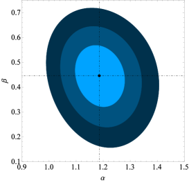
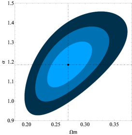
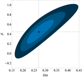
The best fit values of the model parameters $\alpha$ , $\beta$ and $\Omega_{m_{0}}$ have been shown in Table 3. The corresponding contours for $1\sigma$, $2\sigma$ and $3\sigma$ confidence level on $\alpha-\beta(a)$, $\alpha-\Omega_{m_{0}}(b)$ and $\beta-\Omega_{m_{0}}(c)$ planes are also plotted in Figure 2. For simplicity reasons we set $f_{0}=V_{0}=1$. It is interesting that these results are in good agreement with the observational data. It deserves mention here that the value of $\Omega_{m_{0}}$ obtained in the present paper is very close to the expected value.

Data	$\chi_{min}^{2}$	$\Omega_{m_{0}}$	$\alpha$	$\beta$
SN Ia +	584.08	0.270	1.18	0.44
BAO

Table 3: The value of $\chi_{min}^{2}$ and the best fit values of model parameters $\Omega_{m_{0}}$, $\alpha$ and $\beta$ for the second case.

(a)

(b)

(c)

Figure 2: Plots of $1\sigma$ (light blue), $2\sigma$ (blue) and $3\sigma$ (dark blue) confidence contours on $\alpha-\beta$ (a), $\alpha-\Omega_{m_{0}}$ (b) and $\beta-\Omega_{m_{0}}$ (c) parameter spaces for SN Ia+BAO dataset in tachyonic chameleon dark energy scenario with $f(\phi)=f_{0}\phi^{\alpha}$ and $V(\phi)=V_{0}e^{\beta\phi}$. The black dot in each plot shows the best fit point.

4.3 Power-law $f(\phi)$ and $V(\phi)$

In this subsection we obtain observations bounds on the model parameters where $f(\phi)$ and $V(\phi)$ are both in power-law forms as follows:

$$f(\phi) =f_{0}\phi^{\alpha},$$

$$V(\phi) =V_{0}\phi^{\beta}.$$ (16)

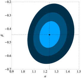
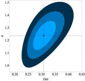
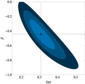
The results for the best fit values of the free parameters of the model i.e. $\alpha$ and $\beta$ together with the present value of $\Omega_{m_{0}}$ extracted from combined analysis SN Ia + BAO are presented in Table 4. In this case the contour plots of various quantities for $68.3\%$, $99.4\%$ and $99.7\%$ confidence level have been shown in Figure 3. As in previous cases we set $f_{0}=V_{0}=1$. One can clearly see that similar to the previous cases this scenario is consistent with observations.

Data	$\chi_{min}^{2}$	$\Omega_{m_{0}}$	$\alpha$	$\beta$
SN Ia +	584.08	0.30	1.23	-0.44
BAO

Table 4: The value of $\chi_{min}^{2}$ and the best fit values of model parameters $\Omega_{m_{0}}$, $\alpha$ and $\beta$ for the third case.

(a)

(b)

(c)

Figure 3: Plots of $1\sigma$ (light blue), $2\sigma$ (blue) and $3\sigma$ (dark blue) confidence contours on $\alpha-\beta$ (a), $\alpha-\Omega_{m_{0}}$ (b) and $\beta-\Omega_{m_{0}}$ (c) parameter spaces for SN Ia+BAO dataset in tachyonic chameleon dark energy scenario with $f(\phi)=f_{0}\phi^{\alpha}$ and $V(\phi)=V_{0}\phi^{\beta}$. The black dot in each plot shows the best fit point.

4.4 Exponential $f(\phi)$ and $V(\phi)$

As a fourth case we obtain observational constraints from combined datasets of SN Ia and BAO on the free parameters of the model where the coupling function and the chameleon potential have exponential forms given by:

$$f(\phi) =f_{0}e^{\alpha\phi},$$

$$V(\phi) =V_{0}e^{\beta\phi}.$$ (17)

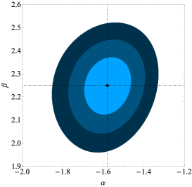
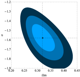
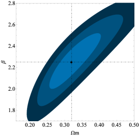
The minimum value of $\chi^{2}$ as well as the best fit values of $\Omega_{m_{0}}$, $\alpha$ and $\beta$ are presented in Table 5. The contour plots of $\alpha$ versus $\beta$, $\Omega_{m_{0}}$ versus $\alpha$ and $\Omega_{m_{0}}$ versus $\beta$ are shown in (a), (b) and (c) panels of Figure 4 respectively. For simplicity reasons we set $f_{0}=V_{0}=1$. As in the previous cases these figures have been plotted for $1\sigma$, $2\sigma$ and $3\sigma$ confidence levels. It is obvious from Figure 4 that the model is in agreement with observational data from SN Ia in combination to BAO.
Before closing this subsection we mention that since the values of the matter density parameter in all cases are very close to each other, $\chi^{2}_{min}$’s are almost the same though the confidence range at each case is different from the others and one can clearly see such a difference in the contours.

Data	$\chi_{min}^{2}$	$\Omega_{m_{0}}$	$\alpha$	$\beta$
SN Ia +	584.09	0.31	-1.58	2.25
BAO

Table 5: The value of $\chi_{min}^{2}$ and the best fit values of model parameters $\Omega_{m_{0}}$, $\alpha$ and $\beta$ for the forth case.

(a)

(b)

(c)

Figure 4: Plots of $1\sigma$ (light blue), $2\sigma$ (blue) and $3\sigma$ (dark blue) confidence contours on $\alpha-\beta$ (a), $\alpha-\Omega_{m}$ (b) and $\beta-\Omega_{m_{0}}$ (c) parameter spaces for SN Ia+BAO dataset in tachyonic chameleon dark energy scenario with $f(\phi)=f_{0}e^{\alpha\phi}$ and $V(\phi)=V_{0}e^{\beta\phi}$. The black dot in each plot shows the best fit point.

5 Conclusion

In this paper we have used the latest observational data to constrain the parameters of the tachyonic chameleon model of dark energy. In our previous paper (Banijamali & Solbi, 2017) we have studied the dynamics of such a scenario and have found that this model has the ability to alleviate the coincidence problem via the mechanism of scaling attractors. Two important functions in our analysis are tachyonic potential $V(\phi)$ and non-minimal coupling function $f(\phi)$ in action (1). In general we have considered two types of these functions i.e power-law and exponential forms.
We have fitted data from Type Ia supernova (SN Ia) and Baryon Acoustic Oscillation (BAO) to constrain the present matter density parameter $\Omega_{m_{0}}$, the parameter $\alpha$ in functional form of $f(\phi)$ (the non-minimal coupling function $f$ is of the form $f(\phi)\propto e^{\alpha\phi}$ or $f(\phi)\propto\phi^{\alpha}$) and the parameter $\beta$ in $V(\phi)$ ( tachyonic potential is assumed to be $V(\phi)\propto e^{\beta\phi}$ or $V(\phi)\propto\phi^{\beta}$). For exponential $f(\phi)$ and power-law $V(\phi)$ we have seen that positive $\alpha$ and negative $\beta$ are favoured by the data while for power-law $f(\phi)$ and exponential $V(\phi)$ both $\alpha$ and $\beta$ should be positive in order to our model be compatible with observations. On the other hand, when $f(\phi)$ and $V(\phi)$ are both power-law functions of scalar field a positive value of $\alpha$ and a negative value of $\beta$ are favoured while when these functions are both in exponential forms then $\alpha$ is negative and $\beta$ is a positive constant. We remark that in all four cases the value of present matter density parameter $\Omega_{m_{0}}$ is very close to the desired value.
In summay, the scenario of the tachyonic chameleon dark energy is compatible with observations, for all examined scalar field potential and non-minimal coupling functions.

References

- [1] Perlmutter, S. et al., Astrophys. J. 517, 565 (1999).
- [2] Riess, A. G. et al., Astron. J. 116, 1009 (1998).
- [3] Ade, P. A. R. et al., A& A. 594, A13 (2016).
- [4] Ade, P. A. R. et al., [BICEP2 Collaboration], Phys. Rev. Lett. 112, 241101 (2014).
- [5] Komatsu, E. et al., [WMAP Collaboration], Astrophys. J. Suppl. 192, 18 (2011).
- [6] Hinshaw, G. et al., [WMAP Collaboration], Astrophys. J. Suppl. 208, 19 (2013).
- [7] Tegmark, M. et al., [SDSS Collaboration], Phys. Rev. D. 69, 103501 (2004).
- [8] Seljak, U. et al. [SDSS Collaboration], Phys. Rev. D. 71, 103515 (2005).
- [9] Eisenstein, D. J. et al., [SDSS Collaboration], Astrophys. J. 633, 560 (2005).
- [10] Jain, B. and Taylor, A., Phys. Rev. Lett. 91, 141302 (2003).
- [11] Ellis, G. F. R. and Madsen, M. S., Class. Quantum Grav. 8, 667 (1991).
- [12] Starobinsky, A. A., JETP Lett. 68, 757 (1998).
- [13] Nojiri, S., Odintsov, S.D. Int.J.Geom.Meth.Mod. 4, 115 (2007).
- [14] Copeland, E.J., Sami, M., Tsujikawa, S., Int. J. Mod. Phys. D. 15, 1753 (2006).
- [15] Nojiri, S., Odintsov, S. D., Phys. Lett. B. 631, 1 (2005).
- [16] Das, S. and Banerjee, N., Phys. Rev. D. 78, 043512 (2008).
- [17] Farajollahi, H., Farhoudi, M. et al., Astrophys. Space Sci. 337, 415 (2012).
- [18] Bisabr, Y., Phys. Rev. D. 86, 127503 (2012).
- [19] Khoury, J., Weltman, A. et al., Phys. Lett. B. 699, 5 (2011).
- [20] Mota, D. F. and Schelpe, C. A. O., Phys. Rev. D. 86, 123002 (2012).
- [21] Banerjee, N., Das, S. and Ganguly, K., Pramana. 74, L481 (2010).
- [22] Khoury, J., Weltman, A. et al., Phys. Rev. D. 70, 123518 (2004).
- [23] Das, S., Corasaniti, P.S. and Khoury, J., Phys. Rev. D. 73, 083509 (2006).
- [24] Khoury, J., Class. Quant. Grav. 30, 214004 (2013).
- [25] Roy, N., Banerjee, N.: Ann. Phys. 452, 356 (2015).
- [26] Banijamali, A. and Solbi, M., Gen Relativ Gravit. 49, 103 (2017).
- [27] Spyros, B., Nesseris, S. and Perivolaropoulos, L. Phys. Rev. D. 87, 123529 (2013).
- [28] Lewis, A. and Bridle, S., Phys. Rev. D. 66, 103511 (2002).
- [29] Yang, L., Lee, C. C., Luo, L. W., Geng, C. Q., Phys. Rev. D. 82, 103515 (2010).
- [30] Li, M., Li, X. D. and Zhang, X., Sci. China Phys. Mech. Astron. 53, 1631 (2010).
- [31] Perivolaropoulos, L., Phys. Rev. D. 71, 063503 (2005).
- [32] Suzuki, N., Rubin, D., Lidman. et al., Astrophys. J. 746 , 85 (2012).
- [33] Percival, W. J. et al., Mon. Not. Roy. Astron. Soc. 401, 2148 (2010).
- [34] Blake, C., Kazin, E., et al., Mon. Not. Roy. Astron. Soc. 418, 1707 (2011).