Signature of Lepton flavor universality violation in $B_{s}\to D_{s}\tau\nu$ semileptonic decays

Abstract

Deviation from the standard model prediction is observed in many semileptonic $B$ decays mediated via $b\to c$ charged current interactions. In particular, current experimental measurements of the ratio of branching ratio $R_{D}$ and $R_{D^{\ast}}$ in $B\rightarrow D^{(*)}l\nu$ decays disagree with standard model expectations at the level of about $4.1\sigma$. Moreover, recent measurement of the ratio of branching ratio $R_{J/\Psi}$ by LHCb, where $R_{J/\Psi}=\mathcal{B}(B_{c}\to J/\Psi\,\tau\nu)/\mathcal{B}(B_{c}\to J/\Psi\,\mu\nu)$, is more than $2\sigma$ away from the standard model prediction. In this context, we consider an effective Lagrangian in the presence of vector and scalar new physics couplings to study the implications of $R_{D}$ and $R_{D^{\ast}}$ anomalies in $B_{s}\to D_{s}\,\tau\nu$ decays. We give prediction of several observables such as branching ratio, ratio of branching ratio, forward backward asymmetry parameter, $\tau$ polarization fraction, and the convexity parameter for the $B_{s}\to D_{s}\,\tau\nu$ decays within the standard model and within various new physics scenarios.

I Introduction

There are several reasons to believe that standard model (SM) of particle physics is not a complete theory, and thus there must be physics beyond the SM. It is therefore crucial to find the pattern of the New Physics (NP) that is responsible for various long standing anomalies. The underlying framework of SM assumes that the charge and neutral leptons are universal in the weak interaction. However, various recent studies on semileptonic $B$ decays such as $B\rightarrow D^{(*)}l\nu$, with $l$ either $e$, $\mu$, or $\tau$, challenged the lepton flavor universality Ciezarek:2017yzh . From past few years, many experiments such as $B-$factories have reported observables that are deviating from the SM prediction. In particular, the ratio of branching ratio $R_{D}$ and $R_{D^{\ast}}$ in $B\rightarrow D^{(*)}l\nu$ are measured to have large discrepancy with respect to its SM counterpart.

A very precise SM prediction of the ratio of branching ratio $R_{D}$ in $B\rightarrow D\,l\,\nu$ using the form factors obtained in lattice quantum chromodynamics (QCD) is reported to be $0.300\pm 0.008$ Lattice:2015rga ; Na:2015kha ; Aoki:2016frl ; Bigi:2016mdz . Similarly for $R_{D^{\ast}}$, it was reported to be $0.252\pm 0.003$ Fajfer:2012vx . Comparing with the current world average of $R_{D}=0.403\pm 0.040\pm 0.024$ and $R_{D^{*}}=0.310\pm 0.015\pm 0.008$ from BABAR Lees:2013uzd , Belle Huschle:2015rga ; Sato:2016svk ; Hirose:2016wfn , and LHCb Aaij:2015yra , the combined deviation currently stands at about $4.1\sigma$. For definiteness, we report in Table-1 the current status of experimentally measured ratio of branching ratio $R_{D}$ and $R_{D^{\ast}}$ Amhis:2016xyh .

Experiments	$R_{D^{\ast}}$	$R_{D}$
BABAR	$0.332\pm 0.024\pm 0.018$	$0.440\pm 0.058\pm 0.042$
BELLE	$0.293\pm 0.038\pm 0.015$	$0.375\pm 0.064\pm 0.026$
BELLE	$0.302\pm 0.030\pm 0.011$
LHCb	$0.336\pm 0.027\pm 0.030$
BELLE	$0.270\pm 0.035^{+0.028}_{-0.025}$
LHCb	$0.285\pm 0.019\pm 0.029$
AVERAGE	$0.304\pm 0.013\pm 0.007$	$0.407\pm 0.039\pm 0.024$

Table 1: Current status of $R_{D}$ and $R_{D^{\ast}}$ Amhis:2016xyh .

Various studies in explaining the observed anomalies in $B$ meson decays can be found in Dutta:2013qaa ; Celis:2012dk ; Dutta:2016eml ; Alok:2016qyh ; Ivanov:2016qtw ; Tran:2017udy ; Celis:2016azn ; Dhargyal:2016nxq ; Colangelo:2018cnj ; Tanaka:1994ay ; Nierste:2008qe ; Miki:2002nz ; Fajfer:2012jt ; Crivellin:2012ye ; Datta:2012qk ; Duraisamy:2013kcw ; Duraisamy:2014sna ; Biancofiore:2013ki ; He:2012zp ; Deshpand:2016cpw ; Li:2016vvp ; Bardhan:2016uhr ; Ivanov:2015tru ; Nandi:2016wlp ; Alonso:2016oyd ; Altmannshofer:2017poe ; Iguro:2017ysu ; Bernlochner:2017jka ; Bhattacharya:2016zcw . Very recently, LHCb has measured the ratio of branching ratio $R_{J/\psi}$ to be $0.71\pm 0.17\pm 0.18$ Aaij:2017tyk . Comparing with the SM prediction Ivanov:2005fd ; Wen-Fei:2013uea ; Dutta:2017xmj , we find the deviation to be at more than $2\sigma$. Although a precise calculation of $B_{c}\to J/\Psi$ form factors is not available at present, a preliminary results for the form factors are provided by HPQCD collaboration using Lattice QCD Lytle:2016ixw .

Inspired by the anomalies present in $B\to(D,\,D^{\ast})\tau\nu$ decays, we study the corresponding $B_{s}\to D_{s}\tau\nu$ semileptonic decays within SM and within various NP scenarios. A systematic study of $B_{s}\to D_{s}\tau\nu$ decays is important for several reasons: first, in the limit of SU(3) flavor symmetry, $B_{s}\to D_{s}\tau\nu$ and $B\to D\tau\nu$ decay modes should show similar properties. Second, since $B\to(D,\,D^{\ast})\tau\nu$ and $B_{s}\to D_{s}\tau\nu$ decays are mediated via $b\to c$ charged current interaction, hence anomalies present in $B\to(D,\,D^{\ast})\tau\nu$ should show up in $B_{s}\to D_{s}\tau\nu$ mode as well. Again, a combined analysis of $B$ and $B_{s}$ meson decays theoretically and experimentally may help us to determine $|V_{cb}|$ with higher precision and this may also give some hints on our understanding of inclusive and exclusive determination of $|V_{cb}|$. The semileptonic $B_{s}\to D_{s}\,l\,\nu$ decays has been studied by various authors Atoui:2013mqa ; Atoui:2013zza ; Bailey:2012rr ; Zhao:2006at ; Bhol:2014jta ; Chen:2011ut ; Li:2010bb ; Fan:2013kqa ; Bazavov:2009bb ; Na:2012kp ; Monahan:2016qxu ; Li:2009wq . Within the SM, the branching ratio and ratio of branching ratio have been calculated using the form factors obtained from perturbative QCD (pQCD), Constituent Quark Meson (CQM) model, covariant light-front quark model, light cone sum rule, and more recently from Lattice QCD. Our main motivation here is to study the implications of $R_{D}$ and $R_{D^{\ast}}$ anomalies on $B_{s}\to D_{s}\tau\nu$ decays in a model independent way. To this end, we use an effective theory formalism in the presence of NP to give prediction on various observables such as the decay rate, ratio of branching ratio, lepton side forward backward asymmetry, longitudinal polarization fraction of the lepton, and the convexity parameter for the $B_{s}\to D_{s}\tau\nu$ decays. We follow Ref. Monahan:2017uby for various $B_{s}\to D_{s}$ transition form factors. For our NP analysis, we impose $1\sigma$ constraint coming from the measured ratio of branching ratio $R_{D}$ and $R_{D^{\ast}}$ to obtain the allowed NP parameter space. This is to ensure that the resulting NP parameter space can simultaneously explain the anomalies present in $R_{D}$ and $R_{D^{\ast}}$. We also use the constraint coming from the $B_{c}$ meson life time in our analysis as it is shown in Ref. Alonso:2016oyd that life time of $B_{c}$ meson put severe constraint on various NP couplings. Based on various SM calculation Bigi:1995fs ; Beneke:1996xe ; Chang:2000ac of the $B_{c}$ life time, it is found that $\mathcal{B}(B_{c}\to\tau\nu)$ can not be more than $5\%$. However, this can be relaxed up to $30\%$ depending on the input parameters that are used in the SM calculation. Very recently, in Ref. Akeroyd:2017mhr a more stringent bound of $\mathcal{B}(B_{c}\to\tau\nu)\leq 10\%$ was obtained using the LEP data at the $Z$ peak.

The present discussion is organized as follows. In section. II, we start with a brief discussion of the most general effective Lagrangian in the presence of NP for the $b\to c\,l\,\nu$ quark level transition decays. The three body differential decay width formula obtained using helicity formalism is also reported in the section. II. Explicit formulas of various observables such as ratio of branching ratio, lepton side forward backward asymmetry, $\tau$ polarization fraction, and the convexity parameter for the $B_{s}\to D_{s}\tau\nu$ decays in the presence of NP are reported. In section. III, we first report all the input parameters that are relevant for our numerical computation. Standard model results and the effects of NP couplings on various observables under various NP scenarios are reported in section. III. Finally, we conclude and summarize our results in section. IV.

II Phenomenology

The natural way to introduce NP effects in a model independent approach is to construct a effective Lagrangian for the weak decays that includes both SM and the beyond the SM physics. We follow Refs. Cirigliano:2009wk ; Bhattacharya:2011qm and write the effective weak Lagrangian for the $b\to c\,\tau\nu$ quark level transition decays in the presence of vector and scalar type NP interactions as

$$\mathcal{L}_{\rm eff} = -\frac{4\,G_{F}}{\sqrt{2}}\,V_{cb}\,\Bigg{\{}(1+V_{L})\,\bar{l}_{L}\,\gamma_{\mu}\,\nu_{L}\,\bar{c}_{L}\,\gamma^{\mu}\,b_{L}+V_{R}\,\bar{l}_{L}\,\gamma_{\mu}\,\nu_{L}\,\bar{c}_{R}\,\gamma^{\mu}\,b_{R}+\widetilde{V}_{L}\,\bar{l}_{R}\,\gamma_{\mu}\,\nu_{R}\,\bar{c}_{L}\,\gamma^{\mu}\,b_{L}$$ (1)

$$+\widetilde{V}_{R}\,\bar{l}_{R}\,\gamma_{\mu}\,\nu_{R}\,\bar{c}_{R}\,\gamma^{\mu}\,b_{R}+S_{L}\,\bar{l}_{R}\,\nu_{L}\,\bar{c}_{R}\,b_{L}+S_{R}\,\bar{l}_{R}\,\nu_{L}\,\bar{c}_{L}\,b_{R}+\widetilde{S}_{L}\,\bar{l}_{L}\,\nu_{R}\,\bar{c}_{R}\,b_{L}+\widetilde{S}_{R}\,\bar{l}_{L}\,\nu_{R}\,\bar{c}_{L}\,b_{R}\Bigg{\}}+{\rm h.c.}\,,$$

where, $G_{F}$ is the Fermi coupling constant and $|V_{cb}|$ is the Cabibbo-Kobayashi-Mashkawa (CKM) matrix element. The effective Lagrangian of Eq. 1 is considered at renormalization scale $\mu=m_{b}$. The NP Wilson coefficients (WCs) denoted by $V_{L}$, $V_{R}$, $S_{L}$, and $S_{R}$ involve left-handed neutrinos, whereas, the WCs denoted by $\tilde{V_{L}}$, $\tilde{V_{R}}$, $\tilde{S_{L}}$, and $\tilde{S_{R}}$ involve right-handed neutrinos, respectively. Assuming all NP WCs to be real in the present analysis we rewrite the above equation as Dutta:2013qaa ,

$$\mathcal{L}_{\rm eff} = -\frac{G_{F}}{\sqrt{2}}\,V_{cb}\,\Bigg{\{}G_{V}\,\bar{l}\,\gamma_{\mu}\,(1-\gamma_{5})\,\nu_{l}\,\bar{c}\,\gamma^{\mu}\,b-G_{A}\,\bar{l}\,\gamma_{\mu}\,(1-\gamma_{5})\,\nu_{l}\,\bar{c}\,\gamma^{\mu}\,\gamma_{5}\,b+G_{S}\,\bar{l}\,(1-\gamma_{5})\,\nu_{l}\,\bar{c}\,b$$ (2)

$$-G_{P}\,\bar{l}\,(1-\gamma_{5})\,\nu_{l}\,\bar{c}\,\gamma_{5}\,b+\widetilde{G}_{V}\,\bar{l}\,\gamma_{\mu}\,(1+\gamma_{5})\,\nu_{l}\,\bar{c}\,\gamma^{\mu}\,b-\widetilde{G}_{A}\,\bar{l}\,\gamma_{\mu}\,(1+\gamma_{5})\,\nu_{l}\,\bar{c}\,\gamma^{\mu}\,\gamma_{5}\,b$$

$$+\widetilde{G}_{S}\,\bar{l}\,(1+\gamma_{5})\,\nu_{l}\,\bar{c}\,b-\widetilde{G}_{P}\,\bar{l}\,(1+\gamma_{5})\,\nu_{l}\,\bar{c}\,\gamma_{5}\,b\Bigg{\}}+{\rm h.c.}\,,$$

where,

$$G_{V}=1+V_{L}+V_{R}\,,\qquad\qquad G_{A}=1+V_{L}-V_{R}\,,\qquad\qquad G_{S}=S_{L}+S_{R}\,,\qquad\qquad G_{P}=S_{L}-S_{R}\,,$$

$$\widetilde{G}_{V}=\widetilde{V}_{L}+\widetilde{V}_{R}\,,\qquad\qquad\widetilde{G}_{A}=\widetilde{V}_{L}-\widetilde{V}_{R}\,,\qquad\qquad\widetilde{G}_{S}=\widetilde{S}_{L}+\widetilde{S}_{R}\,,\qquad\qquad\widetilde{G}_{P}=\widetilde{S}_{L}-\widetilde{S}_{R}\,.$$ (3)

The $B_{s}\to D_{s}\,l\,\nu$ decay amplitude depends on non perturbative hadronic matrix element which can be parametrized in terms of $B_{s}\to D_{s}$ transition form factors as follows.

$$\langle D_{s}(P_{D_{s}})|\bar{c}\,\gamma^{\mu}\,b|B_{s}(P_{B_{s}})\rangle=f_{+}(q^{2})\left[P^{\mu}_{B_{s}}+P^{\mu}_{D_{s}}-\frac{M_{B_{s}}^{2}-M_{D_{s}}^{2}}{q^{2}}q^{\mu}\right]+f_{0}(q^{2})\frac{M_{B_{s}}^{2}-M_{D_{s}}^{2}}{q^{2}}q^{\mu}\,,$$

$$\langle D_{s}(P_{D_{s}})|\bar{c}\,b|B_{s}(P_{B_{s}})\rangle=\frac{m_{B_{s}}^{2}-m_{D_{s}}^{2}}{m_{b}(\mu)-m_{c}(\mu)}\,f_{0}(q^{2})\,,$$ (4)

where, $q^{\mu}=P_{B_{s}}^{\mu}-P_{D_{s}}^{\mu}$ refers to the momentum transfer. It should be mentioned that we use the equation of motion to find the scalar matrix element. We follow Ref. Monahan:2017uby for the relevant form factors $f_{0}(q^{2})$ and $f_{+}(q^{2})$. The expressions pertinent for our discussion are Monahan:2017uby

$$P_{0}(q^{2})f_{0}(q^{2})=\sum_{j=0}^{3}a_{j}^{(0)}\,z^{j}\,,\qquad\qquad P_{+}(q^{2})f_{+}(q^{2})=\sum_{j=0}^{3}a_{j}^{(+)}\,\Big{[}z^{j}-(-1)^{j-J}\frac{j}{J}z^{J}\Big{]}$$ (5)

where

$$z(q^{2})=\frac{\sqrt{t_{+}-q^{2}}-\sqrt{t_{+}-t_{0}}}{\sqrt{t_{+}-q^{2}}+\sqrt{t_{+}-t_{0}}}\,\qquad t_{+}=(M_{B_{s}}+M_{D_{s}})^{2}\,\qquad t_{0}=(M_{B_{s}}-M_{D_{s}})^{2}\,\qquad P_{0,+}(q^{2})=1-\frac{q^{2}}{M_{0,+}^{2}}\,.$$ (6)

Here, $P_{0,+}$ are Blaschke factors and $M_{0}=6.42(10)\,{\rm GeV}$ and $M_{+}=6.330(9)\,{\rm GeV}$ are the resonance masses. We refer to Ref. Monahan:2017uby for all the omitted details.

The differential decay distribution for the $B_{s}\to D_{s}\,l\,\nu$ decays can be expressed as

$$\frac{d\Gamma}{dq^{2}\,d\cos\theta}=\frac{G_{F}^{2}\,|V_{cb}|^{2}\,|\vec{P}_{D_{s}}|}{(2\pi)^{3}\,64\,m_{B_{s}}^{2}}\,\Big{(}1-\frac{m_{l}^{2}}{q^{2}}\Big{)}\,L_{\mu\nu}\,H^{\mu\nu}\,,$$ (7)

where $|\vec{P}_{D_{s}}|=\sqrt{\lambda(m_{B_{s}}^{2},\,m_{D_{s}}^{2},\,q^{2})}/2\,m_{B_{s}}$ is the three momentum vector of the outgoing meson and $\lambda(a,\,b,\,c)=a^{2}+b^{2}+c^{2}-2\,(a\,b+b\,c+c\,a)$. Note that $\theta$ denotes the angle between the $D_{s}$ meson and the lepton three momentum vector in the $(l\,\nu)$ rest frame. The covariant contraction $L_{\mu\nu}H^{\mu\nu}$ can be calculated using the helicity techniques of Refs. Korner:1989qb ; Kadeer:2005aq . For completeness, we present here the final expression for the differential decay distribution of three body $B_{s}\to D_{s}\,l\,\nu$ decays Dutta:2013qaa .

$$\frac{d\Gamma}{dq^{2}\,d\cos\theta}=2\,N\,|\vec{P}_{D_{s}}|\,\Bigg{\{}H_{0}^{2}\,\sin^{2}\theta\,(G_{V}^{2}+\widetilde{G}_{V}^{2})+\frac{m_{l}^{2}}{q^{2}}\,\Big{[}(H_{0}\,G_{V}\,\cos\theta-H_{tS})^{2}+(H_{0}\,\widetilde{G}_{V}\,\cos\theta-\widetilde{H}_{tS})^{2}\Big{]}\Bigg{\}}\,,$$ (8)

where

$$N=\frac{G_{F}^{2}\,|V_{c\,b}|^{2}\,q^{2}}{256\,\pi^{3}\,m_{B_{s}}^{2}}\,\Big{(}1-\frac{m_{l}^{2}}{q^{2}}\Big{)}^{2}\,,\qquad\qquad H_{0}=\frac{2\,m_{B_{s}}\,|\vec{P}_{D_{s}}|}{\sqrt{q^{2}}}\,f_{+}(q^{2})\qquad\qquad H_{t}=\frac{m_{B_{s}}^{2}-m_{D_{s}}^{2}}{\sqrt{q^{2}}}\,f_{0}(q^{2})\,,$$

$$H_{S}=\frac{m_{B_{s}}^{2}-m_{D_{s}}^{2}}{m_{b}(\mu)-m_{c}(\mu)}\,f_{0}(q^{2})\,,\qquad\qquad H_{tS}=H_{t}\,G_{V}+\frac{\sqrt{q^{2}}}{m_{l}}\,H_{S}\,G_{S}\,,\qquad\qquad\widetilde{H}_{tS}=H_{t}\,\widetilde{G}_{V}+\frac{\sqrt{q^{2}}}{m_{l}}\,H_{S}\,\widetilde{G}_{S}\,.$$ (9)

By performing the $\cos\theta$ integration in Eq. 8, we get

$$\frac{d\Gamma}{dq^{2}} = \frac{8\,N\,|\vec{P}_{D_{s}}|\,}{3}\Bigg{\{}\,H_{0}^{2}\,\Big{(}G_{V}^{2}+\widetilde{G}_{V}^{2}\Big{)}\,\Big{(}1+\frac{m_{l}^{2}}{2\,q^{2}}\Big{)}+\frac{3\,m_{l}^{2}}{2\,q^{2}}\,\Big{(}H_{tS}^{2}+\widetilde{H}_{tS}^{2}\Big{)}\Bigg{\}}\,.$$ (10)

Setting $G_{V}=G_{A}=1$ and all other NP couplings to zero, we obtain

$$\Big{(}\frac{d\Gamma}{dq^{2}}\Big{)}_{\rm SM}=\frac{8\,N\,|\vec{P}_{D_{s}}|\,}{3}\Bigg{\{}\,H_{0}^{2}\,\Big{(}1+\frac{m_{l}^{2}}{2\,q^{2}}\Big{)}+\frac{3\,m_{l}^{2}}{2\,q^{2}}\,H_{t}^{2}\Bigg{\}}\,.$$ (11)

We define several $q^{2}$ dependent observables such as differential branching ratio ${\rm DBR}(q^{2})$, ratio of branching ratio $R(q^{2})$, lepton side forward backward asymmetry $A_{FB}^{l}(q^{2})$, polarization fraction of the charged lepton $P_{l}(q^{2})$, and convexity parameter $C_{F}^{l}(q^{2})$ for the $B_{s}\to D_{s}\,l\,\nu$ decays. Those are

$${\rm DBR}(q^{2})=\frac{d\Gamma/dq^{2}}{\Gamma_{\rm Tot}}\,,\qquad\qquad R(q^{2})=\frac{\mathcal{B}(B_{s}\rightarrow D_{s}\tau\nu)}{\mathcal{B}(B_{s}\rightarrow D_{s}\,l\,\nu)}\,,\qquad\qquad A_{FB}(q^{2})=\frac{\Big{(}\int_{-1}^{0}-\int_{0}^{1}\Big{)}d\cos\theta\frac{d\Gamma}{dq^{2}\,d\cos\theta}}{\frac{d\Gamma}{dq^{2}}}\,,$$

$$P_{l}(q^{2})=\frac{d\Gamma(+)/dq^{2}-d\Gamma(-)/dq^{2}}{d\Gamma(+)/dq^{2}+d\Gamma(-)/dq^{2}}\,,\qquad\qquad C_{F}^{l}(q^{2})=\frac{1}{\left(d\Gamma/dq^{2}\right)}\left(\frac{d}{d\cos\theta}\right)^{2}\left[\frac{d\Gamma}{dq^{2}\,d\cos\theta}\right]\,,$$ (12)

where $d\Gamma(+)/dq^{2}$ and $d\Gamma(-)/dq^{2}$ represent differential decay width of positive and negative helicity leptons, respectively. In the presence of various NP, the explicit expressions for $A_{FB}^{l}$, $d\Gamma(+)/dq^{2}$, $d\Gamma(-)/dq^{2}$, and $C_{F}^{l}$ are

$$A_{FB}^{l}(q^{2})=\frac{3m_{l}^{2}}{2q^{2}}\frac{H_{0}\,G_{V}\,H_{tS}+H_{0}\,\widetilde{G}_{V}\,\widetilde{H}_{tS}}{H_{0}^{2}\,(G_{V}^{2}+\widetilde{G}_{V}^{2})\Big{(}1+\frac{m_{l}^{2}}{q^{2}}\Big{)}+\frac{3\,m_{l}^{2}}{2q^{2}}\Big{(}H_{tS}^{2}+\widetilde{H}_{tS}^{2}\Big{)}}\,,$$

$$\frac{d\Gamma(+)}{dq^{2}}=\frac{8\,N|\vec{P_{D_{s}}}|}{3}\Big{[}H_{0}^{2}\,\widetilde{G}_{V}^{2}+\frac{m_{l}^{2}}{2q^{2}}\,\Big{(}H_{0}^{2}\,G_{V}^{2}+3\,H_{tS}^{2}\Big{)}\Big{]}\,$$

$$\frac{d\Gamma(-)}{dq^{2}}=\frac{8\,N|\vec{P_{D_{s}}}|}{3}\Big{[}H_{0}^{2}\,G_{V}^{2}+\frac{m_{l}^{2}}{2q^{2}}\Big{(}H_{0}^{2}\,\tilde{G}_{V}^{2}+3\,\widetilde{H}_{tS}^{2}\Big{)}\Big{]}\,,$$

$$C_{F}^{l}=\frac{3}{2}\frac{H_{0}^{2}\Big{(}G_{V}^{2}+\widetilde{G}_{V}^{2})\Big{(}\frac{m_{l}^{2}}{q^{2}}-1\Big{)}}{\Big{[}H_{0}^{2}\,(G_{V}^{2}+\widetilde{G}_{V}^{2})(1+\frac{m_{l}^{2}}{2\,q^{2}})+\frac{3\,m_{l}^{2}}{2\,q^{2}}(H_{tS}^{2}+\widetilde{H}_{tS}^{2})\Big{]}}$$ (13)

The SM expressions are obtained by setting all the NP couplings to zero.

$$\Big{[}A_{FB}^{l}(q^{2})\Big{]}_{SM}=\frac{3\,m_{l}^{2}}{2\,q^{2}}\Bigg{\{}\frac{H_{0}\,H_{t}}{H_{0}^{2}\,\Big{(}1+\frac{m_{l}^{2}}{q^{2}}\Big{)}+\frac{3\,m_{l}^{2}}{2\,q^{2}}\,H_{t}^{2}}\Bigg{\}}\,,\qquad\Big{[}P^{l}\Big{]}_{SM}=\frac{\frac{m_{l}^{2}}{2\,q^{2}}\,(H_{0}^{2}+3\,H_{t}^{2})-H_{0}^{2}}{\frac{m_{l}^{2}}{2\,q^{2}}\,(H_{0}^{2}+3\,H_{t}^{2})+H_{0}^{2}}\,,$$

$$\Big{[}C_{F}^{l}\Big{]}_{SM}=\frac{3}{2}\frac{H_{0}^{2}\Big{(}\frac{m_{l}^{2}}{q^{2}}-1\Big{)}}{\Big{[}H_{0}^{2}\,\Big{(}1+\frac{m_{l}^{2}}{2\,q^{2}}\Big{)}+\frac{3\,m_{l}^{2}}{2\,q^{2}}\,H_{t}^{2}\Big{]}}$$ (14)

The average values of the forward-backward asymmetry of the charged lepton $<A_{FB}^{l}>$, the longitudinal polarization fraction of the lepton $<P^{l}>$, and the convexity parameter $<C_{F}^{l}>$ are obtained by separately integrating the numerators and denominators over $q^{2}$.

III Numerical results and discussions

III.1 Input parameters

Before proceeding for the analysis, we report in Table-2 all the input parameters that are relevant for our numerical computation. For the mass and lifetime parameter, we use the latest values reported in Ref. Patrignani:2016xqp . Similarly for the CKM matrix element $|V_{cb}|$ and the Fermi coupling constant $G_{F}$, we use Ref. Patrignani:2016xqp . The lepton masses ($m_{e}$, $m_{\tau}$) and meson masses ($B_{s}$, $D_{s}$) are in ${\rm GeV}$ units, whereas Fermi coupling constant $G_{F}$ is in ${\rm GeV}^{-2}$ units. The lifetime of $B_{s}$ meson ($\tau_{B_{s}}$) is in seconds. The quark masses $m_{b}(m_{b})$ and $m_{c}(m_{b})$ evaluated at renormalization scale $\mu=m_{b}$ are in ${\rm GeV}$ units. For the relevant $B_{s}\to D_{s}$ form factor parameters, we follow the most recent Lattice QCD calculation of Ref. Monahan:2017uby . The uncertainties associated with $|V_{cb}|$, and the form factors parameters are written within parenthesis. We do not report the uncertainties associated with other input parameters as they do not play an important role in our analysis.

Inputs from PDG  Patrignani:2016xqp		Form factor inputs  Monahan:2017uby
$m_{B_{s}}$	5.36689	$a_{0}^{(0)}$	0.658(31)
$m_{D_{s}}$	1.96827	$a_{1}^{(0)}$	-0.10(30)
$m_{b}(\mu)$	4.18	$a_{2}^{(0)}$	1.3(2.8)
$m_{c}(\mu)$	0.91	$a_{0}^{(+)}$	0.858(32)
$m_{e}$	0.05109989461$\times 10^{-2}$	$a_{1}^{(+)}$	-3.38(41)
$m_{\tau}$	1.77682	$a_{2}^{(+)}$	0.6(4.7)
$|V_{cb}|$	0.0409(11)
$G_{F}$	$1.1663787\times 10^{-5}$
$\tau_{B_{s}}$	$1.505\times 10^{-12}$

Table 2: Theory inputs

We wish to determine the consequences of various NP couplings on various observables for the $B_{s}\to D_{s}\tau\nu$ decays in a model independent way. It is, therefore, crucial to determine the size of the SM uncertainties in each observable that may come from various input parameters. Uncertainties in the theoretical prediction of the observables mainly come from two sources. First, it may come from not very well known CKM matrix element $|V_{cb}|$ and second, it may come from the non perturbative hadronic inputs such as decay constant and meson to meson form factors. To gauge the effect of above mentioned uncertainties on various observables, we use a random number generator and vary these input parameters within $1\sigma$ of their central values.

III.2 Standard model prediction

First, we wish to give prediction of various observables for both the $e$ and $\tau$ mode within the SM. We report in Table.-3 the SM central values and the $1\sigma$ ranges of each observable for the $e$ and the $\tau$ modes. Here, the central values are obtained by considering only the central values of theory input parameters whereas, the $1\sigma$ ranges of each observable is obtained by performing a random scan of the hadronic parameters and the CKM matrix element within $1\sigma$ of their central values. The value of ratio of branching ratio $R_{D_{s}}$ in Table.-3 is quite similar to the value reported in Ref. Monahan:2017uby . The slight difference may come from different choices of input parameters.

Observables	Central value	$1\sigma$ range	Observables	Central value	$1\sigma$ range	Observables	Central value	$1\sigma$ range
$\mathcal{B}(B_{s}\to D_{s}\,e\nu)\%$	$2.238$	$[1.839,2.693]$	$P^{e}$	$-1.00$	$-1.00$	$P^{\tau}$	$0.320$	$[0.234,0.403]$
$\mathcal{B}(B_{s}\to D_{s}\tau\nu)\%$	$0.670$	$[0.573,0.777]$	$A^{e}_{FB}$	$0.00$	$0.00$	$A^{\tau}_{FB}$	$0.360$	$[0.352,0.364]$
$R_{D_{s}}$	$0.299$	$[0.260,0.351]$	$C^{e}_{F}$	$-1.5$	$-1.50$	$C^{\tau}_{F}$	$-0.271$	$[-0.239,-0.305]$

Table 3: SM prediction of various observables for the $e$ and the $\tau$ modes

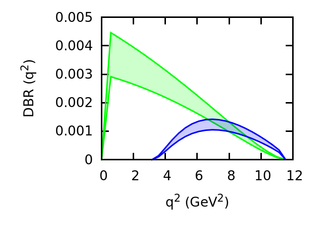
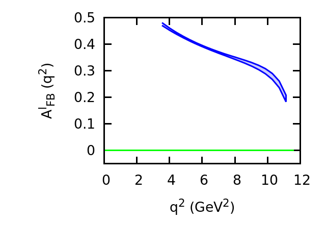
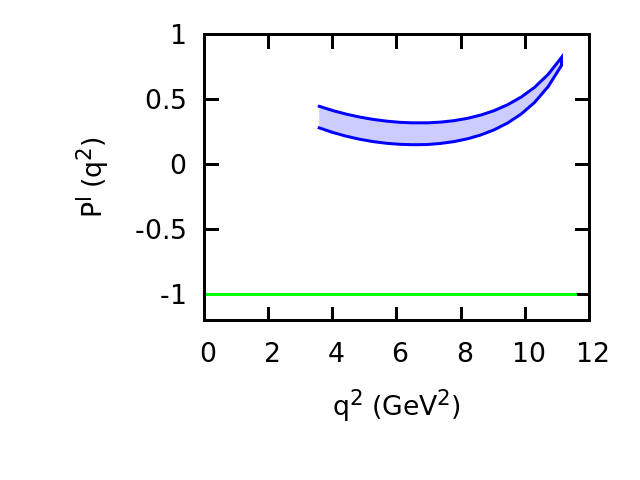
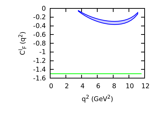
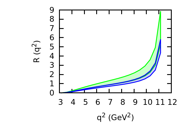
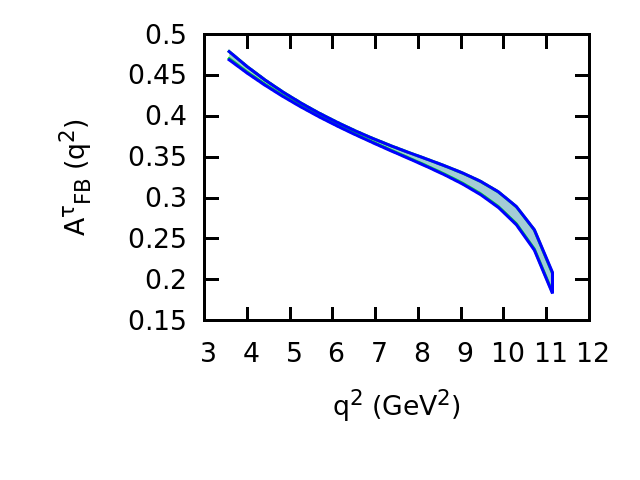
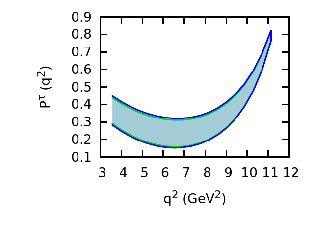
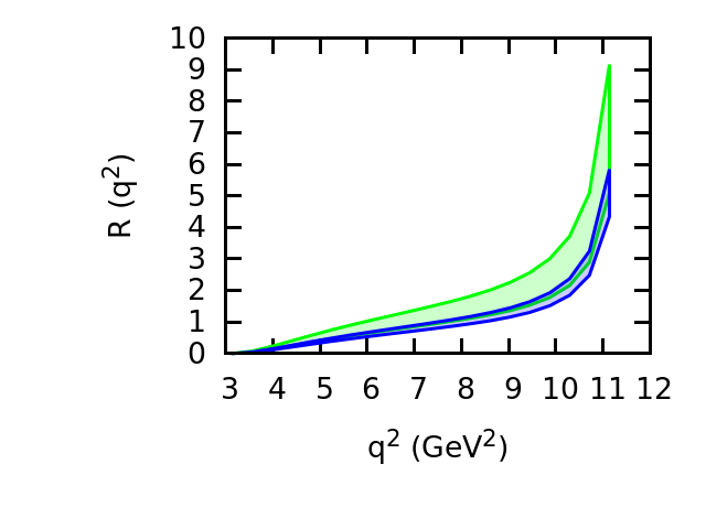
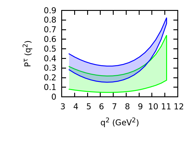
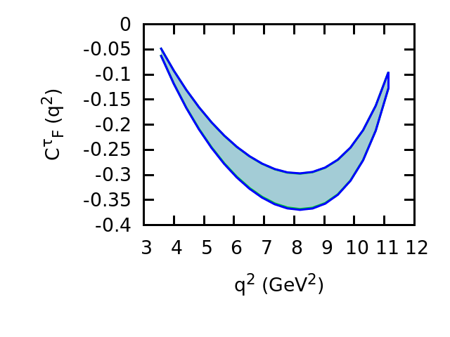
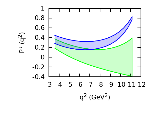
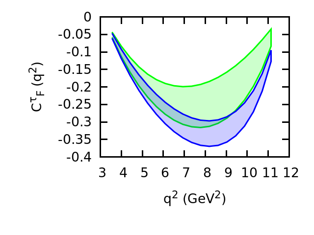
We notice that the SM prediction for the $e$ mode is quite different from the $\tau$ mode. There is even a sign change in the polarization fraction $P_{l}$ while going from the $e$ to the $\tau$ mode. Again, the forward backward asymmetry parameter for the $e$ mode is zero, whereas, it is non zero positive for the $\tau$ mode. Similarly, the convexity parameter $C_{F}^{l}$ for the $e$ mode is much larger in magnitude than for the $\tau$ mode. It is worth mentioning that the mass of the charged lepton plays an important role. In Fig. 1, we show the $q^{2}$ dependence of each observable for the $e$ and the $\tau$ modes, respectively. We notice that the $A_{FB}^{l}(q^{2})$, $P^{l}(q^{2})$ and the $C_{F}^{l}(q^{2})$ observables remain constant in the entire $q^{2}$ region for the $e$ mode. This could be very well understood from Eq. II. In the massless limit, i.e, in the $m_{l}\to 0$ limit, the $q^{2}$ dependence gets cancelled in the ratio for the $A_{FB}^{l}(q^{2})$, $P^{l}(q^{2})$ and the $C_{F}^{l}(q^{2})$ observables.

Figure 1: $q^{2}$ dependence of various observables in the SM for the $e$ (green) and the $\tau$ (blue) modes.

Now we proceed to discuss various NP effects in $B_{s}\to D_{s}\,\tau\,\nu$ decays.

III.3 New physics in $B_{s}\to D_{s}\,\tau\,\nu$ decays

Study of $B_{s}\to D_{s}\,\tau\,\nu$ decays both theoretically and experimentally is well motivated because of the long standing anomalies present in $R_{D}$ and $R_{D^{\ast}}$. We wish to study the implication of these existing anomalies on the $B_{s}\to D_{s}\,\tau\,\nu$ decays in a model independent way. We consider four different NP scenarios based on NP contributions from two different operators. In order to determine the allowed NP parameter space, we impose $1\sigma$ constraint coming from the measured ratio of branching ratios $R_{D}$ and $R_{D^{\ast}}$. We use the average values of $R_{D}$ and $R_{D^{\ast}}$ reported in Table. 1 in our analysis. For the uncertainties we added the statistical and systematic uncertainties in quadrature. Again, we assume that only the third generation leptons get contribution from NP.

III.3.1 Scenario I: only $V_{L}$ and $V_{R}$ NP couplings

In this scenario, we vary $V_{L}$ and $V_{R}$ and set all other NP couplings to zero. This is to ensure that NP contribution to the $B_{s}\to D_{s}\tau\nu$ decay mode is coming only from vector type NP couplings that involves left handed neutrinos. In the presence of such NP, the $d\Gamma/dq^{2}$, $R(q^{2})$, $A_{FB}^{\tau}(q^{2})$, $P^{\tau}(q^{2})$, and $C^{\tau}_{F}(q^{2})$ can be expressed as

$$\left[\frac{d\Gamma}{dq^{2}}\right]_{V_{L,R}}=\left[\frac{d\Gamma}{dq^{2}}\right]_{SM}G_{V}^{2}\,,\qquad\qquad\left[R_{D_{s}}\right]_{V_{L.R}}=\left[R_{D_{s}}\right]_{SM}G_{V}^{2}\,,$$

$$\left[A_{FB}^{l}(q^{2})\right]_{V_{L,R}}=\left[A_{FB}^{l}(q^{2})\right]_{SM}\,,\qquad\qquad\left[P^{l}\right]_{V_{L,R}}=\left[P^{l}\right]_{SM}\,,\qquad\qquad\left[C_{F}^{l}\right]_{V_{L,R}}=\left[C_{F}^{l}\right]_{SM}$$ (15)

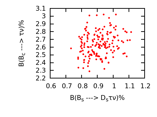
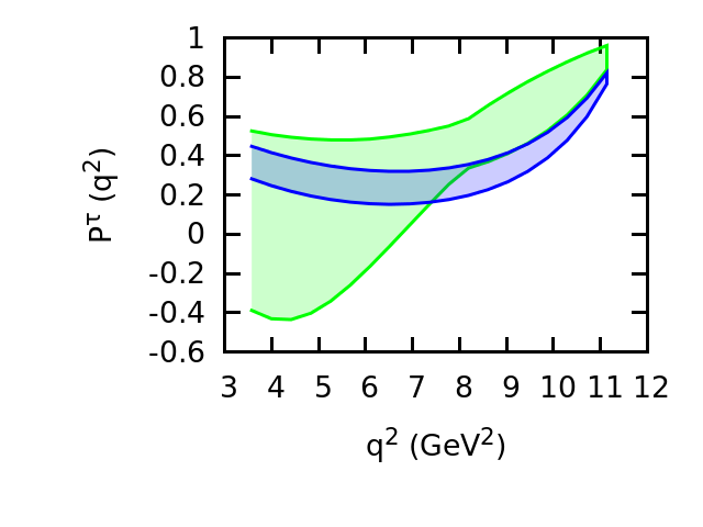
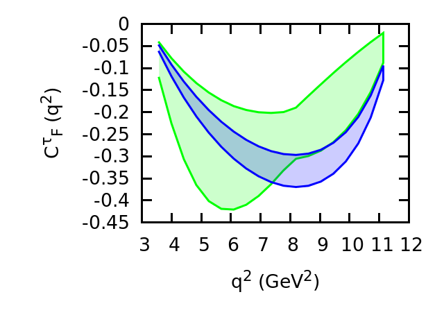
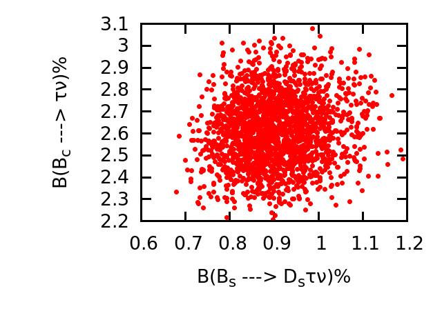
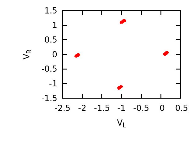
It is evident from Eq. III.3.1 that $d\Gamma/dq^{2}$ and $R(q^{2})$ depend on $V_{L}$ and $V_{R}$ NP couplings and are proportional to $G_{V}^{2}$, whereas, $P^{\tau}(q^{2})$, $A^{\tau}_{FB}(q^{2})$, and $C^{\tau}_{F}(q^{2})$ do not depend on these NP couplings since the contribution coming from $V_{L}$ and $V_{R}$ NP couplings gets canceled in the ratio. The allowed ranges of $V_{L}$ and $V_{R}$ after imposing $1\sigma$ constraint coming from $R_{D}$ and $R_{D^{\ast}}$ are shown in the left panel of Fig. 2. In the right panel we show the corresponding ranges in $\mathcal{B}(B_{c}\to\tau\nu)$ and $\mathcal{B}(B_{s}\to D_{s}\tau\nu)$. From the right panel of Fig. 2, we notice that the $\mathcal{B}(B_{c}\to\tau\nu)$ obtained in this scenario lies in the $2\%-3\%$ range. This is consistent with the SM calculation.

Figure 2: Allowed ranges of $V_{L}$ and $V_{R}$ NP couplings are shown in the left panel once $1\sigma$ constraint coming from the measured values of the ratio of branching ratios $R_{D}$ and $R_{D^{\ast}}$ is imposed. We show in the right panel the allowed ranges in $\mathcal{B}(B_{c}\to\tau\nu)$ and $\mathcal{B}(B_{s}\to D_{s}\tau\nu)$ in the presence of these NP couplings.

We report in Table-4 the allowed ranges of each observable for the $B_{s}\rightarrow D_{s}\tau\nu$ decays with $(V_{L}$, $V_{R})$ NP couplings of Fig. 2. We see significant deviation in $\mathcal{B}(B_{s}\to D_{s}\tau\nu)$ and $R_{D_{s}}$ from the SM prediction. As expected, the ranges of $P^{\tau}_{D_{s}}$, $A^{\tau}_{FB}$, and $C^{\tau}_{F}$ do not vary at all with such NP couplings.

$\mathcal{B}(B_{s}\to D_{s}\tau\nu)\%$	$R_{D_{s}}$	$P^{\tau}$	$A^{\tau}_{FB}$	$C^{\tau}_{F}$
$[0.733,1.115]$	$[0.329,0.496]$	$[0.234,0.403]$	$[0.352,0.364]$	$[-0.239,-0.305]$

Table 4: Allowed ranges of various observables with $V_{L}$ and $V_{R}$ NP couplings of Fig. 2.

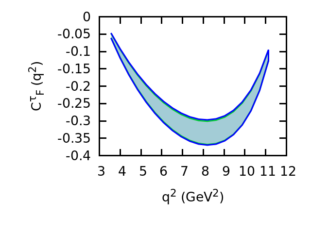
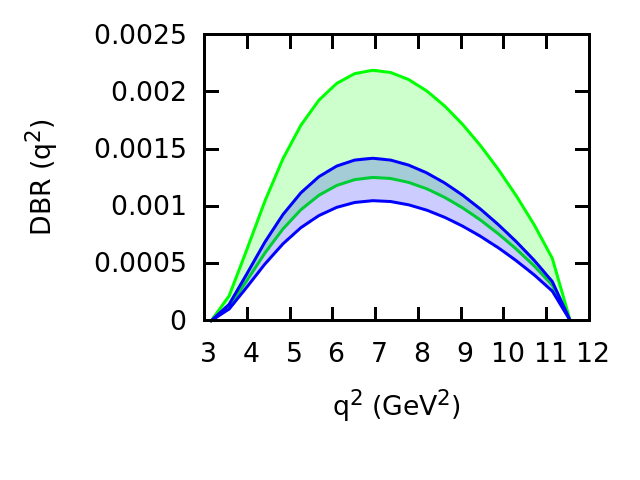
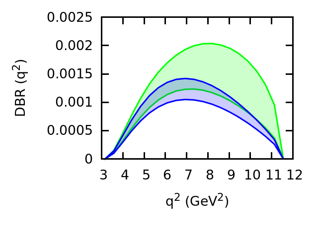
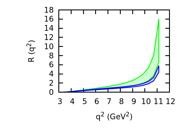
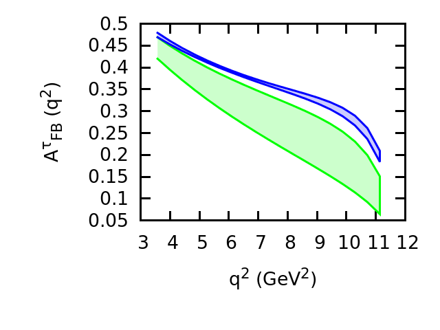
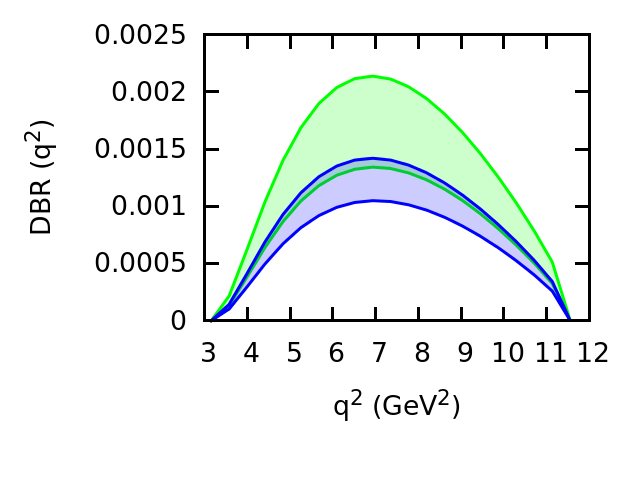
Figure 3: $q^{2}$ dependence of various observables with the allowed ranges of $V_{L}$ and $V_{R}$ NP couplings of Fig. 2 are shown with green band. The corresponding $1\sigma$ SM range is shown with the blue band.

We show in Fig. 3 the $q^{2}$ dependence of various observables with the allowed values of $V_{L}$ and $V_{R}$ NP couplings of Fig. 2. The SM $1\sigma$ range is shown with blue band, whereas, the allowed range with $V_{L}$ and $V_{R}$ NP couplings is shown with green band. It is evident from Fig. 3 that the differential branching ratio ${\rm DBR}(q^{2})$ and ratio of branching ratio $R(q^{2})$ deviate considerably from the SM expectation. Again, as expected, we do not observe any deviation of $A_{FB}^{\tau}(q^{2})$, $P_{\tau}(q^{2})$ and $C_{F}^{\tau}(q^{2})$ from the SM expectation in this NP scenario.

III.3.2 Scenario II: only $S_{L}$ and $S_{R}$ NP couplings

In this scenario, we consider the effect of new scalar couplings only, i.e,$(S_{L},\,S_{R})\neq 0$ and all the other NP couplings are zero. In the presence of $S_{L}$ and $S_{R}$ NP couplings, the differential decay width, ratio of branching ratio, forward backward asymmetry, polarization fraction of the $\tau$ lepton, and the convexity parameter can be expressed as

$$\left[\frac{d\Gamma}{dq^{2}}\right]_{S_{L,R}}=\left[\frac{d\Gamma}{dq^{2}}\right]_{SM}+8N|P_{D_{s}}|\left(\frac{1}{2}H_{S}^{2}\,{G}_{S}^{2}+\frac{m_{l}}{\sqrt{q^{2}}}H_{t}\,H_{S}\,G_{S}\,\right),$$

$$\left[R_{D_{s}}\right]_{S_{L,R}}=\left[R_{D_{s}}\right]_{SM}+\frac{8N|P_{D_{s}}|\left(\frac{1}{2}H_{S}^{2}\,{G}_{S}^{2}+\frac{m_{l}}{\sqrt{q^{2}}}H_{t}\,H_{S}\,G_{S}\,\right)}{\mathcal{B}(B_{s}\to D_{s}\,e\,\nu)}\,,$$

$$A_{FB}^{l}(q^{2})|_{S_{L,R}}=\frac{3\,m_{l}^{2}}{2\,q^{2}}\left[\frac{H_{0}\,H_{t}+H_{0}\,\frac{\sqrt{q^{2}}}{m_{l}}\,H_{S}\,G_{S}}{H_{0}^{2}\,\Big{(}1+\frac{m_{l}^{2}}{q^{2}}\Big{)}+\frac{3\,m_{l}^{2}}{2\,q^{2}}H_{t}^{2}+(3/2)\,H_{S}^{2}\,G_{S}^{2}+3\,(m_{l}/\sqrt{q^{2}})\,H_{t}\,H_{S}\,G_{S}}\right]\,,$$

$$\left[P^{l}\right]_{S_{L,R}}=\frac{\frac{m_{l}^{2}}{2\,q^{2}}\,(H_{0}^{2}+3\,H_{t}^{2})-H_{0}^{2}+(3/2)\,H_{S}^{2}\,G_{S}^{2}+3\,(m_{l}/\sqrt{q^{2}})\,H_{t}\,H_{S}\,G_{S}}{\frac{m_{l}^{2}}{2\,q^{2}}(H_{0}^{2}+3\,H_{t}^{2})+H_{0}^{2}+(3/2)\,H_{S}^{2}\,G_{S}^{2}+3\,(m_{l}/\sqrt{q^{2}})\,H_{t}\,H_{S}\,G_{S}}\,,$$

$$\left[C_{F}^{l}\right]_{S_{L,R}}=\frac{3}{2}\frac{H_{0}^{2}\left(\frac{m_{l}^{2}}{q^{2}}-1\right)}{\left\{H_{0}^{2}\Big{(}1+\frac{m_{l}^{2}}{2q^{2}}\Big{)}+\frac{3\,m_{l}^{2}}{2\,q^{2}}\,H_{t}^{2}\right\}+(3/2)\,H_{S}^{2}\,G_{S}^{2}+3\,(m_{l}/\sqrt{q^{2}})\,H_{t}\,H_{S}\,G_{S}}$$ (16)

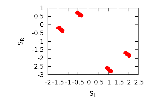
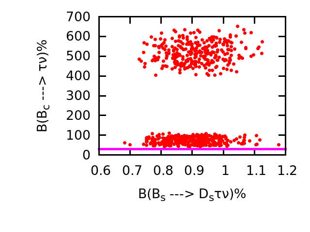
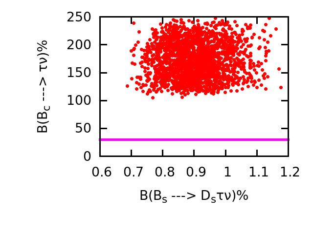
We impose $1\sigma$ constraint coming from experimental values of $R_{D}$ and $R_{D^{\ast}}$ to determine the allowed values of $S_{L}$ and $S_{R}$ NP couplings. The resulting $(S_{L},\,S_{R})$ allowed ranges are shown in the left panel of Fig. 4.. In the right panel, we show the corresponding ranges in $\mathcal{B}(B_{c}\to\tau\nu)$ and $\mathcal{B}(B_{s}\to D_{s}\tau\nu)$ obtained using the allowed values of $(S_{L},\,S_{R})$ NP couplings. It should be noted that the $\mathcal{B}(B_{c}\to\tau\nu)$ obtained in this scenario is rather large; more than $30\%$. Thus, although $(S_{L},\,S_{R})$ NP couplings can simultaneously explain the anomalies present in $R_{D}$ and $R_{D^{\ast}}$, it, however, fails to satisfy the $\mathcal{B}(B_{c}\to\tau\nu)\leq 30\%$ constraint obtained in the SM.

Figure 4: Allowed ranges of $S_{L}$ and $S_{R}$ NP couplings are shown in the left panel once $1\sigma$ constraint coming from the measured values of the ratio of branching ratios $R_{D}$ and $R_{D^{\ast}}$ is imposed. We show in the right panel the allowed ranges in $\mathcal{B}(B_{c}\to\tau\nu)$ and $\mathcal{B}(B_{s}\to D_{s}\tau\nu)$ in the presence of these NP couplings. The pink constant line in the right panel corresponds to the upper bound of $\mathcal{B}(B_{c}\to\tau\nu)=30\%$ obtained in the SM.

$\mathcal{B}(B_{s}\to D_{s}\tau\nu)\%$	$R_{D_{s}}$	$P^{\tau}$	$A^{\tau}_{FB}$	$C^{\tau}_{F}$
$[0.683,1.178]$	$[0.306,0.518]$	$[0.345,0.609]$	$[-0.276,0.355]$	$[-0.156,-0.260]$

Table 5: Allowed ranges of various observables in the presence of $S_{L}$ and $S_{R}$ NP couplings

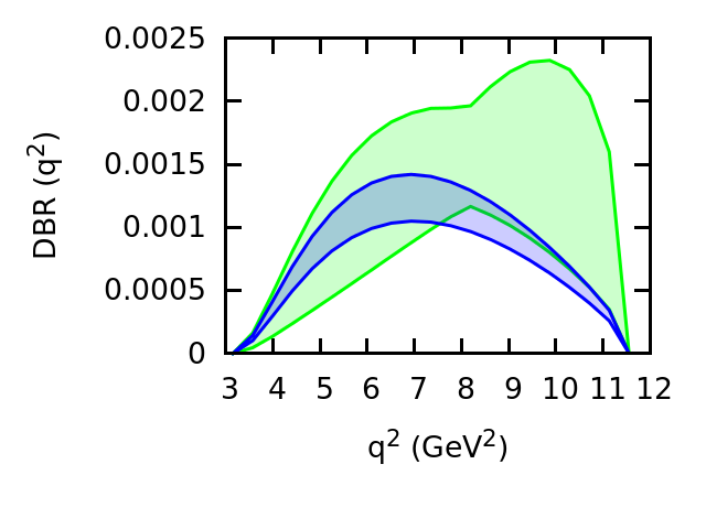
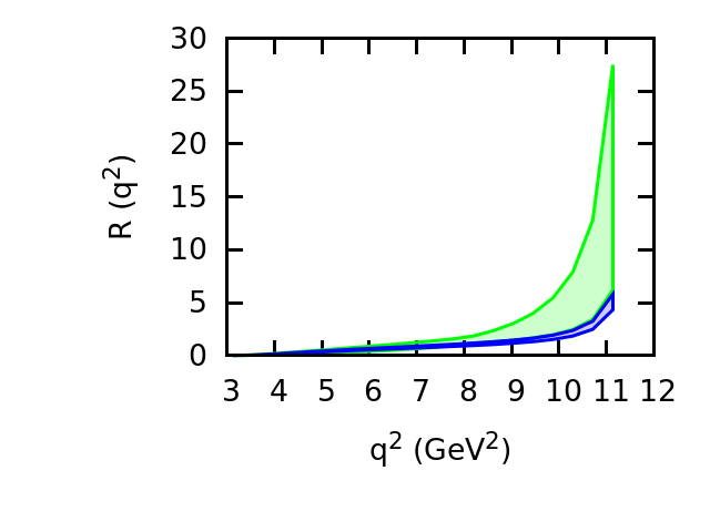
Although this particular scenario is ruled out by the $\mathcal{B}(B_{c}\to\tau\nu)$ constraint, nevertheless, we report in Table. 5 the allowed ranges of all the observables obtained using the allowed values of $S_{L}$ and $S_{R}$ NP couplings of Fig. 4. The deviation from the SM prediction observed in this scenario is quite significant. We notice that the forward backward asymmetry parameter can assume negative values within this scenario, which is quite distinct from SM expectation.

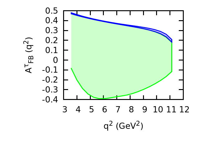
Figure 5: $q^{2}$ dependence of various observables with the allowed ranges of $S_{L}$ and $S_{R}$ NP couplings of Fig. 4 are shown with green band. The corresponding $1\sigma$ SM range is shown with the blue band.

We show the effect of NP on various $q^{2}$ dependent observables in Fig. 5. We show with blue the SM $1\sigma$ band, whereas, we show with green the allowed band once the NP is switched on. The deviation observed in this scenario is rather large and it is, indeed, more pronounced that the deviation obtained with $(V_{L},\,V_{R})$ NP couplings. Unlike scenario I, there is no cancellation of NP effects in $A_{FB}^{\tau}(q^{2})$, $P^{\tau}(q^{2})$, and $C_{F}^{\tau}(q^{2})$. We notice that, although there is no zero crossing in the SM for the $A_{FB}^{\tau}(q^{2})$ parameter, we may observe zero crossing depending on the values of $S_{L}$ and $S_{R}$ NP couplings. Similar conclusion can be drawn for the $\tau$ polarization fraction $P^{\tau}(q^{2})$ as well. Moreover, depending on the values of the NP couplings, shape of the $q^{2}$ distribution curve of each observable can be quite different from its SM counterpart.

III.3.3 Scenario III: only $\widetilde{V}_{L}$ and $\widetilde{V}_{R}$ NP couplings

To study the effect of new vector type NP couplings associated with right handed neutrino interactions, we consider $(\widetilde{V}_{L},\,\widetilde{V}_{R})$ to be nonzero while all other NP couplings to be zero. In this scenario, the differential decay width, ratio of branching ratio, forward backward asymmetry, $\tau$ polarization fraction, and the convexity parameter take the following simple form:

$$\left[\frac{d\Gamma}{dq^{2}}\right]_{\widetilde{V}_{L,R}}=\left[\frac{d\Gamma}{dq^{2}}\right]_{SM}(1+\widetilde{G}_{V}^{2})\,,\qquad\qquad\left[R_{D_{s}}\right]_{\widetilde{V}_{L,R}}=\left[R_{D_{s}}\right]_{SM}(1+\widetilde{G}_{V}^{2})\,,$$

$$\left[A_{FB}^{l}(q^{2})\right]_{\widetilde{V}_{L,R}}=\left[A_{FB}^{l}(q^{2})\right]_{SM}\,,\qquad\qquad\left[P^{l}\right]_{\widetilde{V}_{L,R}}=\left[P^{l}\right]_{SM}\frac{(1-\widetilde{G}_{V}^{2})}{(1+\widetilde{G}_{V}^{2})}\,,\qquad\qquad\left[C_{F}^{l}\right]_{\widetilde{V}_{L,R}}=\left[C_{F}^{l}\right]_{SM}$$ (17)

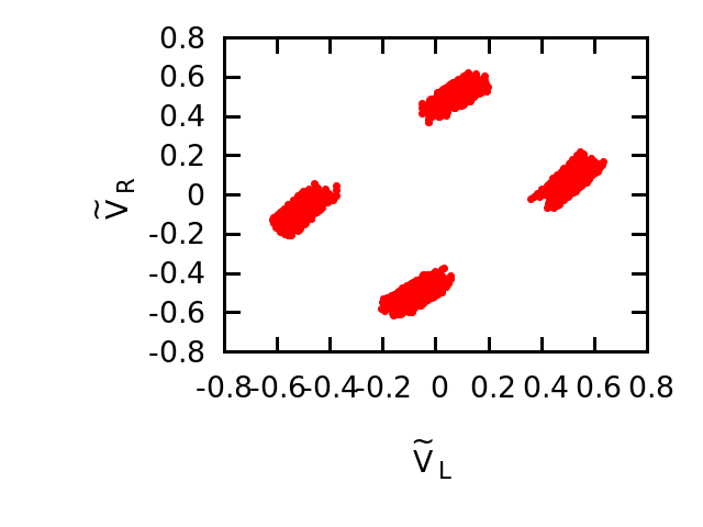
In the left panel of Fig. 6 we show the allowed region of $(\widetilde{V}_{L}$, $\widetilde{V}_{R})$ NP couplings that is obtained once $1\sigma$ $R_{D}$ and $R_{D^{\ast}}$ experimental constraint is imposed. Similarly, in the right panel we show the corresponding ranges of $\mathcal{B}(B_{c}\to\tau\nu)$ and $\mathcal{B}(B_{s}\to D_{s}\tau\nu)$ obtained with the $(\widetilde{V}_{L}$, $\widetilde{V}_{R})$ NP couplings. Similar to Scenario I, we notice that $\mathcal{B}(B_{c}\to\tau\nu)$ obtained in this scenario lies within $(2-3)\%$ range. This is, again, consistent with the SM prediction. In Table. 6, we report the possible ranges of all the observables for the $B_{s}\to D_{s}\tau\nu$ decays. The deviation from the SM prediction observed in this scenario is quite similar to the deviation observed in scenario I. However, there is one subtle difference. Unlike scenario I, a significant deviation from the SM prediction for the $\tau$ polarization fraction is observed in this scenario. This is evident from Eq. III.3.3 that the NP effect does not get cancelled for the $\tau$ polarization fraction $P^{\tau}$.

In Fig. 7, we show the variation of various observables such as differential branching ratio, ratio of branching ratio, forward-backward asymmetry, $\tau$ polarization fraction, and convexity parameter as a function of $q^{2}$. The deviation from the SM prediction observed in this scenario is quite similar to scenario I. As expected, we observe a significant deviation in $\tau$ polarization parameter in this scenario. All the above mentioned analysis for the observed deviations are clearly reflected in Eq. III.3.3.

Figure 6: Allowed ranges of $\widetilde{V}_{L}$ and $\widetilde{V}_{R}$ NP couplings are shown in the left panel once $1\sigma$ constraint coming from the measured values of the ratio of branching ratios $R_{D}$ and $R_{D^{\ast}}$ is imposed. We show in the right panel the allowed ranges in $\mathcal{B}(B_{c}\to\tau\nu)$ and $\mathcal{B}(B_{s}\to D_{s}\tau\nu)$ in the presence of these NP couplings.

$\mathcal{B}(B_{s}\to D_{s}\tau\nu)\%$	$R_{D_{s}}$	$P^{\tau}$	$A^{\tau}_{FB}$	$C^{\tau}_{F}$
$[0.679,1.191]$	$[0.305,0.525]$	$[0.064,0.281]$	$[0.352,0.364]$	$[-0.239,-0.305]$

Table 6: Allowed ranges of various observables in the presence of $\widetilde{V}_{L}$ and $\widetilde{V}_{R}$ NP couplings

Figure 7: $q^{2}$ dependence of various observables with the allowed ranges of $\widetilde{V}_{L}$ and $\widetilde{V}_{R}$ NP couplings of Fig. 6 are shown with green band. The corresponding $1\sigma$ SM range is shown with the blue band.

III.3.4 Scenario IV: only $\widetilde{S}_{L}$ and $\widetilde{S}_{R}$ NP couplings

In this scenario, we wish to see the effect of new scalar type NP couplings on various observables. To this end, we consider $(\widetilde{S}_{L},\widetilde{S}_{R})$ to be non zero and all other NP couplings to be zero. In this scenario, the differential decay width, ratio of branching ratio, forward backward asymmetry, $\tau$ polarization fraction, and the convexity parameter take the following form:

$$\left[\frac{d\Gamma}{dq^{2}}\right]_{\widetilde{S}_{L,R}}=\left[\frac{d\Gamma}{dq^{2}}\right]_{SM}+4\,N|P_{D_{s}}|H_{S}^{2}\,\widetilde{G}_{S}^{2}\,,\qquad\qquad\left[R_{D_{s}}\right]_{\widetilde{S}_{L,R}}=\left[R_{D_{s}}\right]_{SM}+\frac{(3/2)\,H_{S}^{2}\,\widetilde{G}_{S}^{2}}{\mathcal{B}(B_{s}\to D_{s}\,e\,\nu)}\,,$$

$$\left[A_{FB}^{l}(q^{2})\right]_{\widetilde{S}_{L,R}}=\frac{3\,m_{l}^{2}}{2\,q^{2}}\left[\frac{H_{0}\,H_{t}}{H_{0}^{2}\,\Big{(}1+\frac{m_{l}^{2}}{q^{2}}\Big{)}+\frac{3\,m_{l}^{2}}{2\,q^{2}}H_{t}^{2}+(3/2)\,H_{S}^{2}\,\widetilde{G}_{S}^{2}}\right]\,,$$

$$\left[P^{l}\right]_{\widetilde{S}_{L,R}}=\frac{\frac{m_{l}^{2}}{2\,q^{2}}(H_{0}^{2}+3\,H_{t}^{2})-H_{0}^{2}-(3/2)\,H_{S}^{2}\widetilde{G}_{S}^{2}}{\frac{m_{l}^{2}}{2\,q^{2}}(H_{0}^{2}+3\,H_{t}^{2})+H_{0}^{2}+(3/2)\,H_{S}^{2}\widetilde{G}_{S}^{2}}\,,$$

$$\left[C_{F}^{l}(q^{2})\right]_{\widetilde{S}_{L,R}}=\frac{3}{2}\frac{H_{0}^{2}\left(\frac{m_{l}^{2}}{q^{2}}-1\right)}{\left\{H_{0}^{2}\Big{(}1+\frac{m_{l}^{2}}{2\,q^{2}}\Big{)}+\frac{3\,m_{l}^{2}}{2\,q^{2}}\,H_{t}^{2}\right\}+(3/2)\,H_{S}^{2}\widetilde{G}_{S}^{2}}$$ (18)

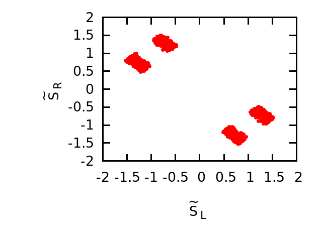
In order to determine the allowed ranges of $(\widetilde{S}_{L},\widetilde{S}_{R})$ NP couplings, we impose $1\sigma$ constraint coming from experimentally measured values of $R_{D}$ and $R_{D^{\ast}}$. The resulting NP parameter space, shown in the left panel of Fig. 8, can simultaneously explain the anomalies present in $R_{D}$ and $R_{D^{\ast}}$. We show in the right panel the allowed ranges in $\mathcal{B}(B_{c}\to\tau\nu)$ and $B_{s}\to D_{s}\tau\nu$ with such NP. We notice that the $\mathcal{B}(B_{c}\to\tau\nu)$ obtained in this scenario is not compatible with the upper bound of $\mathcal{B}(B_{c}\to\tau\nu)\leq 30\%$ obtained in the SM. The numerical values written in the square brackets of Table-7 represent the allowed ranges of observables obtained with the allowed values of $(\widetilde{S}_{L},\widetilde{S}_{R})$ of Fig. 8. Similar to scenario II, we see significant deviation of all the observables from the SM expectation.

We show in Fig. 9 the $q^{2}$ distribution of various observables for the $B_{s}\to D_{s}\tau\nu$ decays. The blue band corresponds to the $1\sigma$ SM range, whereas, the green band corresponds to the range of the observables once the $(\widetilde{S}_{L},\widetilde{S}_{R})$ NP couplings are switched on. The deviation observed in this scenario is rather large. We notice that although, in the SM, there is no zero crossing in the $\tau$ polarization parameter, there may or may not be a zero crossing depending on the values of the NP couplings. For the differential branching ratio, the peak of the $q^{2}$ distribution may shift towards high $q^{2}$ region.

Figure 8: Allowed ranges of $\widetilde{S}_{L}$ and $\widetilde{S}_{R}$ NP couplings are shown in the left panel once $1\sigma$ constraint coming from the measured values of the ratio of branching ratios $R_{D}$ and $R_{D^{\ast}}$ is imposed. The corresponding allowed ranges in $\mathcal{B}(B_{c}\to\tau\nu)$ and $\mathcal{B}(B_{s}\to D_{s}\tau\nu)$ in the presence of such NP couplings are shown in the right panel. The pink constant line denotes the upper bound of $\mathcal{B}(B_{c}\to\tau\nu)=30\%$ obtained in the SM.

$\mathcal{B}(B_{s}\to D_{s}\tau\nu)\%$	$R_{D_{s}}$	$P^{\tau}$	$A^{\tau}_{FB}$	$C^{\tau}_{F}$
$[0.687,1.176]$	$[0.305,0.532]$	$[-0.201,0.205]$	$[0.219,0.331]$	$[-0.155,-0.261]$

Table 7: Allowed ranges of various observables in the presence of $\widetilde{S}_{L}$ and $\widetilde{S}_{R}$ NP couplings

Figure 9: $q^{2}$ dependence of various observables with the allowed ranges of $\widetilde{S}_{L}$ and $\widetilde{S}_{R}$ NP couplings of Fig. 8 are shown with green band. The corresponding $1\sigma$ SM range is shown with the blue band.

IV Conclusion

In view of the long standing anomalies in $R_{D}$ and $R_{D^{\ast}}$, we study the corresponding $B_{s}\to D_{s}\tau\nu$ semileptonic decays in a model independent framework. We use the helicity formalism to study the $B_{s}\to D_{s}\tau\nu$ semileptonic decays within the context of an effective Lagrangian in the presence of NP and explore four different NP scenarios based on contributions coming from two different NP operators. We give prediction on various observables such as branching ratio, ratio of branching ratio, forward backward asymmetry, longitudinal polarization fraction of the charged lepton, and the convexity parameter for this decay mode within SM and within four different NP scenarios.

We first report the central values and the $1\sigma$ ranges of each observable within the SM for both the $e$ and the $\tau$ modes. We notice that all the observables change considerably while going from the $e$ mode to the $\tau$ mode. The value of $R_{D_{s}}$ is quite similar to the value reported in Ref. Monahan:2017uby . We also give the first prediction of the longitudinal polarization fraction of the charged lepton, lepton side forward backward asymmetry, and the convexity parameter for the $B_{s}\to D_{s}\,l\,\nu$ decays.

For our NP analysis, we assume that NP effects are coming from vector and scalar type NP couplings only. We notice that NP scenarios with $(V_{L},\,V_{R})$ and $(\widetilde{V}_{L},\,\widetilde{V}_{R})$ NP couplings are compatible with the $\mathcal{B}(B_{c}\to\tau\nu)$ constraint. However, NP scenarios with $(S_{L},\,S_{R})$ and $(\widetilde{S}_{L},\,\widetilde{S}_{R})$ NP couplings are ruled out due to the constraint coming from the lifetime of $B_{c}$ meson.

Study of $B_{s}\to D_{s}\tau\nu$ decays both theoretically and experimentally is crucial because it may provide new insights into the $R_{D}$ and $R_{D^{\ast}}$ anomaly as this decay mode is mediated via the same $b\to c$ charged current interaction. Moreover, a precise determination of the branching fractions of this decay mode will allow an accurate determination of the CKM matrix element $|V_{cb}|$.

References

• (1) G. Ciezarek, M. Franco Sevilla, B. Hamilton, R. Kowalewski, T. Kuhr, V. Lüth and Y. Sato, “A Challenge to Lepton Universality in B Meson Decays,” Nature 546, 227 (2017) doi:10.1038/nature22346 [arXiv:1703.01766 [hep-ex]].
• (2) J. A. Bailey et al. [MILC Collaboration], “B→Dℓν form factors at nonzero recoil and |Vcb|subscript𝑉𝑐𝑏|V_{cb}| from 2+1-flavor lattice QCD,” Phys. Rev. D 92, no. 3, 034506 (2015) doi:10.1103/PhysRevD.92.034506 [arXiv:1503.07237 [hep-lat]].
• (3) H. Na et al. [HPQCD Collaboration], “BDlν𝐵𝐷𝑙𝜈B\rightarrow Dl\nu form factors at nonzero recoil and extraction of |Vcb|subscript𝑉𝑐𝑏|V_{cb}|,” Phys. Rev. D 92, no. 5, 054510 (2015) Erratum: [Phys. Rev. D 93, no. 11, 119906 (2016)] doi:10.1103/PhysRevD.93.119906, 10.1103/PhysRevD.92.054510 [arXiv:1505.03925 [hep-lat]].
• (4) S. Aoki et al., “Review of lattice results concerning low-energy particle physics,” Eur. Phys. J. C 77, no. 2, 112 (2017) doi:10.1140/epjc/s10052-016-4509-7 [arXiv:1607.00299 [hep-lat]].
• (5) D. Bigi and P. Gambino, “Revisiting BDν𝐵𝐷𝜈B\to D\ell\nu,” Phys. Rev. D 94, no. 9, 094008 (2016) doi:10.1103/PhysRevD.94.094008 [arXiv:1606.08030 [hep-ph]].
• (6) S. Fajfer, J. F. Kamenik and I. Nisandzic, “On the BDτν¯τ𝐵superscript𝐷𝜏subscript¯𝜈𝜏B\to D^{*}\tau\bar{\nu}_{\tau} Sensitivity to New Physics,” Phys. Rev. D 85, 094025 (2012) doi:10.1103/PhysRevD.85.094025 [arXiv:1203.2654 [hep-ph]].
• (7) J. P. Lees et al. [BaBar Collaboration], “Measurement of an Excess of B¯D()τν¯τ¯𝐵superscript𝐷superscript𝜏subscript¯𝜈𝜏\bar{B}\to D^{(*)}\tau^{-}\bar{\nu}_{\tau} Decays and Implications for Charged Higgs Bosons,” Phys. Rev. D 88, no. 7, 072012 (2013) doi:10.1103/PhysRevD.88.072012 [arXiv:1303.0571 [hep-ex]].
• (8) M. Huschle et al. [Belle Collaboration], “Measurement of the branching ratio of B¯D()τν¯τ¯𝐵superscript𝐷superscript𝜏subscript¯𝜈𝜏\bar{B}\to D^{(\ast)}\tau^{-}\bar{\nu}_{\tau} relative to B¯D()ν¯¯𝐵superscript𝐷superscriptsubscript¯𝜈\bar{B}\to D^{(\ast)}\ell^{-}\bar{\nu}_{\ell} decays with hadronic tagging at Belle,” Phys. Rev. D 92, no. 7, 072014 (2015) doi:10.1103/PhysRevD.92.072014 [arXiv:1507.03233 [hep-ex]].
• (9) Y. Sato et al. [Belle Collaboration], “Measurement of the branching ratio of B¯0D+τν¯τsuperscript¯𝐵0superscript𝐷absentsuperscript𝜏subscript¯𝜈𝜏\bar{B}^{0}\rightarrow D^{*+}\tau^{-}\bar{\nu}_{\tau} relative to B¯0D+ν¯superscript¯𝐵0superscript𝐷absentsuperscriptsubscript¯𝜈\bar{B}^{0}\rightarrow D^{*+}\ell^{-}\bar{\nu}_{\ell} decays with a semileptonic tagging method,” Phys. Rev. D 94, no. 7, 072007 (2016) doi:10.1103/PhysRevD.94.072007 [arXiv:1607.07923 [hep-ex]].
• (10) S. Hirose et al. [Belle Collaboration], “Measurement of the τ𝜏\tau lepton polarization and R(D)𝑅superscript𝐷R(D^{*}) in the decay B¯Dτν¯τ¯𝐵superscript𝐷superscript𝜏subscript¯𝜈𝜏\bar{B}\to D^{*}\tau^{-}\bar{\nu}_{\tau},” Phys. Rev. Lett.  118, no. 21, 211801 (2017) doi:10.1103/PhysRevLett.118.211801 [arXiv:1612.00529 [hep-ex]].
• (11) R. Aaij et al. [LHCb Collaboration], “Measurement of the ratio of branching fractions (B¯0D+τν¯τ)/(B¯0D+μν¯μ)superscript¯𝐵0superscript𝐷absentsuperscript𝜏subscript¯𝜈𝜏superscript¯𝐵0superscript𝐷absentsuperscript𝜇subscript¯𝜈𝜇\mathcal{B}(\bar{B}^{0}\to D^{*+}\tau^{-}\bar{\nu}_{\tau})/\mathcal{B}(\bar{B}^{0}\to D^{*+}\mu^{-}\bar{\nu}_{\mu}),” Phys. Rev. Lett.  115, no. 11, 111803 (2015) Erratum: [Phys. Rev. Lett.  115, no. 15, 159901 (2015)] doi:10.1103/PhysRevLett.115.159901, 10.1103/PhysRevLett.115.111803 [arXiv:1506.08614 [hep-ex]].
• (12) Y. Amhis et al. [HFLAV Collaboration], “Averages of b𝑏b-hadron, c𝑐c-hadron, and τ𝜏\tau-lepton properties as of summer 2016,” Eur. Phys. J. C 77, no. 12, 895 (2017) doi:10.1140/epjc/s10052-017-5058-4 [arXiv:1612.07233 [hep-ex]].
• (13) R. Dutta, A. Bhol and A. K. Giri, “Effective theory approach to new physics in bu𝑏𝑢b\to u and bc𝑏𝑐b\to c leptonic and semileptonic decays,” Phys. Rev. D 88, no. 11, 114023 (2013) doi:10.1103/PhysRevD.88.114023 [arXiv:1307.6653 [hep-ph]].
• (14) A. Celis, M. Jung, X. Q. Li and A. Pich, “Sensitivity to charged scalars in 𝑩𝑫()𝝉𝝂𝝉bold-→𝑩superscript𝑫𝝉subscript𝝂𝝉\bm{B\to D^{(*)}\tau\nu_{\tau}} and 𝑩𝝉𝝂𝝉bold-→𝑩𝝉subscript𝝂𝝉\bm{B\to\tau\nu_{\tau}} decays,” JHEP 1301, 054 (2013) doi:10.1007/JHEP01(2013)054 [arXiv:1210.8443 [hep-ph]].
• (15) R. Dutta and A. Bhol, “b(c,u),τν𝑏𝑐𝑢𝜏𝜈b\to(c,u),\tau\nu leptonic and semileptonic decays within an effective field theory approach,” Phys. Rev. D 96, no. 3, 036012 (2017) doi:10.1103/PhysRevD.96.036012 [arXiv:1611.00231 [hep-ph]].
• (16) A. K. Alok, D. Kumar, S. Kumbhakar and S. U. Sankar, “Dsuperscript𝐷D^{*} polarization as a probe to discriminate new physics in B¯Dτν¯¯𝐵superscript𝐷𝜏¯𝜈\bar{B}\to D^{*}\tau\bar{\nu},” Phys. Rev. D 95, no. 11, 115038 (2017) doi:10.1103/PhysRevD.95.115038 [arXiv:1606.03164 [hep-ph]].
• (17) M. A. Ivanov, J. G. Körner and C. T. Tran, “Analyzing new physics in the decays B¯0D()τν¯τsuperscript¯𝐵0superscript𝐷superscript𝜏subscript¯𝜈𝜏\bar{B}^{0}\to D^{(\ast)}\tau^{-}\bar{\nu}_{\tau} with form factors obtained from the covariant quark model,” Phys. Rev. D 94, no. 9, 094028 (2016) doi:10.1103/PhysRevD.94.094028 [arXiv:1607.02932 [hep-ph]].
• (18) C. T. Tran, M. A. Ivanov and J. G. Körner, “Analyzing New Physics in B¯0D()τν¯τsuperscript¯𝐵0superscript𝐷superscript𝜏subscript¯𝜈𝜏\bar{B}^{0}\to D^{(\ast)}\tau^{-}\bar{\nu}_{\tau},” arXiv:1702.06910 [hep-ph].
• (19) A. Celis, M. Jung, X. Q. Li and A. Pich, “Scalar contributions to bc(u)τν𝑏𝑐𝑢𝜏𝜈b\to c(u)\tau\nu transitions,” Phys. Lett. B 771, 168 (2017) doi:10.1016/j.physletb.2017.05.037 [arXiv:1612.07757 [hep-ph]].
• (20) L. Dhargyal, “Explaining the observed deviation in R(D()superscript𝐷D^{(*)}) and Br(Bτντ𝐵𝜏subscript𝜈𝜏B\to\tau\nu_{\tau}) in an anomalous 2HDM,” arXiv:1610.06291 [hep-ph].
• (21) P. Colangelo and F. De Fazio, “Scrutinizing B¯D(Dπ)ν¯¯𝐵superscript𝐷𝐷𝜋superscriptsubscript¯𝜈\bar{B}\to D^{*}(D\pi)\ell^{-}\bar{\nu}_{\ell} and B¯D(Dγ)ν¯¯𝐵superscript𝐷𝐷𝛾superscriptsubscript¯𝜈\bar{B}\to D^{*}(D\gamma)\ell^{-}\bar{\nu}_{\ell} in search of new physics footprints,” arXiv:1801.10468 [hep-ph].
• (22) M. Tanaka, “Charged Higgs effects on exclusive semitauonic B𝐵B decays,” Z. Phys. C 67, 321 (1995) doi:10.1007/BF01571294 [hep-ph/9411405].
• (23) U. Nierste, S. Trine and S. Westhoff, “Charged-Higgs effects in a new B —¿ D tau nu differential decay distribution,” Phys. Rev. D 78, 015006 (2008) doi:10.1103/PhysRevD.78.015006 [arXiv:0801.4938 [hep-ph]].
• (24) T. Miki, T. Miura and M. Tanaka, “Effects of charged Higgs boson and QCD corrections in anti-B —¿ D tau anti-nu(tau),” hep-ph/0210051.
• (25) S. Fajfer, J. F. Kamenik, I. Nisandzic and J. Zupan, “Implications of Lepton Flavor Universality Violations in B Decays,” Phys. Rev. Lett.  109, 161801 (2012) doi:10.1103/PhysRevLett.109.161801 [arXiv:1206.1872 [hep-ph]].
• (26) A. Crivellin, C. Greub and A. Kokulu, “Explaining BDτν𝐵𝐷𝜏𝜈B\to D\tau\nu, BDτν𝐵superscript𝐷𝜏𝜈B\to D^{*}\tau\nu and Bτν𝐵𝜏𝜈B\to\tau\nu in a 2HDM of type III,” Phys. Rev. D 86, 054014 (2012) doi:10.1103/PhysRevD.86.054014 [arXiv:1206.2634 [hep-ph]].
• (27) A. Datta, M. Duraisamy and D. Ghosh, “Diagnosing New Physics in bcτντ𝑏𝑐𝜏subscript𝜈𝜏b\to c\,\tau\,\nu_{\tau} decays in the light of the recent BaBar result,” Phys. Rev. D 86, 034027 (2012) doi:10.1103/PhysRevD.86.034027 [arXiv:1206.3760 [hep-ph]].
• (28) M. Duraisamy and A. Datta, “The Full BDτντ¯𝐵superscript𝐷superscript𝜏¯subscript𝜈𝜏B\to D^{*}\tau^{-}\bar{\nu_{\tau}} Angular Distribution and CP violating Triple Products,” JHEP 1309, 059 (2013) doi:10.1007/JHEP09(2013)059 [arXiv:1302.7031 [hep-ph]].
• (29) M. Duraisamy, P. Sharma and A. Datta, “Azimuthal BDτντ¯𝐵superscript𝐷superscript𝜏¯subscript𝜈𝜏B\to D^{*}\tau^{-}\bar{\nu_{\tau}} angular distribution with tensor operators,” Phys. Rev. D 90, no. 7, 074013 (2014) doi:10.1103/PhysRevD.90.074013 [arXiv:1405.3719 [hep-ph]].
• (30) P. Biancofiore, P. Colangelo and F. De Fazio, “On the anomalous enhancement observed in BD()τν¯τ𝐵superscript𝐷𝜏subscript¯𝜈𝜏B\to D^{(*)}\tau{\bar{\nu}}_{\tau} decays,” Phys. Rev. D 87, no. 7, 074010 (2013) doi:10.1103/PhysRevD.87.074010 [arXiv:1302.1042 [hep-ph]].
• (31) X. G. He and G. Valencia, “B𝐵B decays with τ𝜏\tau leptons in nonuniversal left-right models,” Phys. Rev. D 87, no. 1, 014014 (2013) doi:10.1103/PhysRevD.87.014014 [arXiv:1211.0348 [hep-ph]].
• (32) N. G. Deshpande and X. G. He, “Consequences of R-parity violating interactions for anomalies in B¯D()τν¯¯𝐵superscript𝐷𝜏¯𝜈\bar{B}\to D^{(*)}\tau\bar{\nu} and bsμ+μ𝑏𝑠superscript𝜇superscript𝜇b\to s\mu^{+}\mu^{-},” Eur. Phys. J. C 77, no. 2, 134 (2017) doi:10.1140/epjc/s10052-017-4707-y [arXiv:1608.04817 [hep-ph]].
• (33) X. Q. Li, Y. D. Yang and X. Zhang, “Revisiting the one leptoquark solution to the R(D(∗)) anomalies and its phenomenological implications,” JHEP 1608, 054 (2016) doi:10.1007/JHEP08(2016)054 [arXiv:1605.09308 [hep-ph]].
• (34) D. Bardhan, P. Byakti and D. Ghosh, “A closer look at the RD and RDsuperscript𝐷{}_{D^{*}} anomalies,” JHEP 1701, 125 (2017) doi:10.1007/JHEP01(2017)125 [arXiv:1610.03038 [hep-ph]].
• (35) M. A. Ivanov, J. G. Körner and C. T. Tran, “Exclusive decays Bν¯𝐵superscript¯𝜈B\to\ell^{-}\bar{\nu} and BD()ν¯𝐵superscript𝐷superscript¯𝜈B\to D^{(\ast)}\ell^{-}\bar{\nu} in the covariant quark model,” Phys. Rev. D 92, no. 11, 114022 (2015) doi:10.1103/PhysRevD.92.114022 [arXiv:1508.02678 [hep-ph]].
• (36) S. Nandi, S. K. Patra and A. Soni, “Correlating new physics signals in BD()τντ𝐵superscript𝐷𝜏subscript𝜈𝜏B\to D^{(*)}\tau\nu_{\tau} with Bτντ𝐵𝜏subscript𝜈𝜏B\to\tau\nu_{\tau},” arXiv:1605.07191 [hep-ph].
• (37) R. Alonso, B. Grinstein and J. Martin Camalich, “Lifetime of Bcsuperscriptsubscript𝐵𝑐B_{c}^{-} Constrains Explanations for Anomalies in BD()τν𝐵superscript𝐷𝜏𝜈B\to D^{(*)}\tau\nu,” Phys. Rev. Lett.  118, no. 8, 081802 (2017) doi:10.1103/PhysRevLett.118.081802 [arXiv:1611.06676 [hep-ph]].
• (38) W. Altmannshofer, P. S. Bhupal Dev and A. Soni, “RD()subscript𝑅superscript𝐷R_{D^{(*)}} anomaly: A possible hint for natural supersymmetry with R𝑅R-parity violation,” Phys. Rev. D 96, no. 9, 095010 (2017) doi:10.1103/PhysRevD.96.095010 [arXiv:1704.06659 [hep-ph]].
• (39) S. Iguro and K. Tobe, “R(D())𝑅superscript𝐷R(D^{(*)}) in a general two Higgs doublet model,” Nucl. Phys. B 925, 560 (2017) doi:10.1016/j.nuclphysb.2017.10.014 [arXiv:1708.06176 [hep-ph]].
• (40) F. U. Bernlochner, Z. Ligeti, M. Papucci and D. J. Robinson, “Combined analysis of semileptonic B𝐵B decays to D𝐷D and Dsuperscript𝐷D^{*}: R(D())𝑅superscript𝐷R(D^{(*)}), |Vcb|subscript𝑉𝑐𝑏|V_{cb}|, and new physics,” Phys. Rev. D 95, no. 11, 115008 (2017) doi:10.1103/PhysRevD.95.115008 [arXiv:1703.05330 [hep-ph]].
• (41) S. Bhattacharya, S. Nandi and S. K. Patra, “Looking for possible new physics in BD()τντ𝐵superscript𝐷𝜏subscript𝜈𝜏B\to D^{(\ast)}\tau\nu_{\tau} in light of recent data,” Phys. Rev. D 95, no. 7, 075012 (2017) doi:10.1103/PhysRevD.95.075012 [arXiv:1611.04605 [hep-ph]].
• (42) R. Aaij et al. [LHCb Collaboration], “Measurement of the ratio of branching fractions (Bc+J/ψτ+ντ)superscriptsubscript𝐵𝑐𝐽𝜓superscript𝜏subscript𝜈𝜏\mathcal{B}(B_{c}^{+}\,\to\,J/\psi\tau^{+}\nu_{\tau})/(Bc+J/ψμ+νμ)superscriptsubscript𝐵𝑐𝐽𝜓superscript𝜇subscript𝜈𝜇\mathcal{B}(B_{c}^{+}\,\to\,J/\psi\mu^{+}\nu_{\mu}),” arXiv:1711.05623 [hep-ex].
• (43) M. A. Ivanov, J. G. Korner and P. Santorelli, “Semileptonic decays of Bcsubscript𝐵𝑐B_{c} mesons into charmonium states in a relativistic quark model,” Phys. Rev. D 71, 094006 (2005) Erratum: [Phys. Rev. D 75, 019901 (2007)] doi:10.1103/PhysRevD.75.019901, 10.1103/PhysRevD.71.094006 [hep-ph/0501051].
• (44) W. F. Wang, Y. Y. Fan and Z. J. Xiao, “Semileptonic decays Bc(ηc,J/Ψ)lνsubscript𝐵𝑐subscript𝜂𝑐𝐽Ψ𝑙𝜈B_{c}\to(\eta_{c},J/\Psi)l\nu in the perturbative QCD approach,” Chin. Phys. C 37, 093102 (2013) doi:10.1088/1674-1137/37/9/093102 [arXiv:1212.5903 [hep-ph]].
• (45) R. Dutta and A. Bhol, “Bc(J/ψ,ηc)τνsubscript𝐵𝑐𝐽𝜓subscript𝜂𝑐𝜏𝜈B_{c}\to(J/\psi,\,\eta_{c})\tau\nu semileptonic decays within the standard model and beyond,” Phys. Rev. D 96, no. 7, 076001 (2017) doi:10.1103/PhysRevD.96.076001 [arXiv:1701.08598 [hep-ph]].
• (46) A. Lytle, B. Colquhoun, C. Davies, J. Koponen and C. McNeile, PoS BEAUTY 2016, 069 (2016) [arXiv:1605.05645 [hep-lat]].
• (47) M. Atoui, D. Becirevic, V. Morénas and F. Sanfilippo, “Lattice QCD study of BsDsν¯subscript𝐵𝑠subscript𝐷𝑠subscript¯𝜈B_{s}\to D_{s}\ell\bar{\nu}_{\ell} decay near zero recoil,” PoS LATTICE 2013, 384 (2014) [arXiv:1311.5071 [hep-lat]].
• (48) M. Atoui, V. Morénas, D. Bečirevic and F. Sanfilippo, “BsDsνsubscript𝐵𝑠subscript𝐷𝑠subscript𝜈B_{s}\to D_{s}\ell\nu_{\ell} near zero recoil in and beyond the Standard Model,” Eur. Phys. J. C 74, no. 5, 2861 (2014) doi:10.1140/epjc/s10052-014-2861-z [arXiv:1310.5238 [hep-lat]].
• (49) J. A. Bailey et al., “BsDs/BDsubscript𝐵𝑠subscript𝐷𝑠𝐵𝐷B_{s}\to D_{s}/B\to D Semileptonic Form-Factor Ratios and Their Application to BR(Bs0μ+μsubscriptsuperscript𝐵0𝑠superscript𝜇superscript𝜇B^{0}_{s}\to\mu^{+}\mu^{-}),” Phys. Rev. D 85, 114502 (2012) Erratum: [Phys. Rev. D 86, 039904 (2012)] doi:10.1103/PhysRevD.85.114502, 10.1103/PhysRevD.86.039904 [arXiv:1202.6346 [hep-lat]].
• (50) S. M. Zhao, X. Liu and S. J. Li, “Study on B(s) —¿ D(sJ) (2317, 2460) l anti-nu Semileptonic Decays in the CQM Model,” Eur. Phys. J. C 51, 601 (2007) doi:10.1140/epjc/s10052-007-0322-7 [hep-ph/0612008].
• (51) A. Bhol, “Study of Bs \to Ds(∗)lνlsubscript𝜈𝑙\nu_{l} semileptonic decays,” EPL 106, no. 3, 31001 (2014). doi:10.1209/0295-5075/106/31001
• (52) X. J. Chen, H. F. Fu, C. S. Kim and G. L. Wang, “Estimating Form Factors of BsDs()subscript𝐵𝑠superscriptsubscript𝐷𝑠B_{s}\rightarrow D_{s}^{(*)} and their Applications to Semi-leptonic and Non-leptonic Decays,” J. Phys. G 39, 045002 (2012) doi:10.1088/0954-3899/39/4/045002 [arXiv:1106.3003 [hep-ph]].
• (53) G. Li, F. l. Shao and W. Wang, “BsDs(3040)subscript𝐵𝑠subscript𝐷𝑠3040B_{s}\to D_{s}(3040) form factors and Bssubscript𝐵𝑠B_{s} decays into Ds(3040)subscript𝐷𝑠3040D_{s}(3040),” Phys. Rev. D 82, 094031 (2010) doi:10.1103/PhysRevD.82.094031 [arXiv:1008.3696 [hep-ph]].
• (54) Y. Y. Fan, W. F. Wang and Z. J. Xiao, “Study of B¯s0(Ds+,Ds+)lν¯lsuperscriptsubscript¯𝐵𝑠0superscriptsubscript𝐷𝑠superscriptsubscript𝐷𝑠absentsuperscript𝑙subscript¯𝜈𝑙\bar{B}_{s}^{0}\to(D_{s}^{+},D_{s}^{*+})l^{-}\bar{\nu}_{l} decays in the pQCD factorization approach,” Phys. Rev. D 89, no. 1, 014030 (2014) doi:10.1103/PhysRevD.89.014030 [arXiv:1311.4965 [hep-ph]].
• (55) A. Bazavov et al. [MILC Collaboration], “Nonperturbative QCD Simulations with 2+1 Flavors of Improved Staggered Quarks,” Rev. Mod. Phys.  82, 1349 (2010) doi:10.1103/RevModPhys.82.1349 [arXiv:0903.3598 [hep-lat]].
• (56) H. Na, C. J. Monahan, C. T. H. Davies, R. Horgan, G. P. Lepage and J. Shigemitsu, “The B𝐵B and Bssubscript𝐵𝑠B_{s} Meson Decay Constants from Lattice QCD,” Phys. Rev. D 86, 034506 (2012) doi:10.1103/PhysRevD.86.034506 [arXiv:1202.4914 [hep-lat]].
• (57) C. J. Monahan, H. Na, C. M. Bouchard, G. P. Lepage and J. Shigemitsu, “B(s)D(s)subscript𝐵𝑠subscript𝐷𝑠B_{(s)}\to D_{(s)} semileptonic decays with NRQCD-HISQ valence quarks,” PoS LATTICE 2016, 298 (2016) [arXiv:1611.09667 [hep-lat]].
• (58) R. H. Li, C. D. Lu and Y. M. Wang, “Exclusive B(s)𝐵𝑠B(s) decays to the charmed mesons D(s)+(1968,2317)𝐷𝑠19682317D(s)+(1968,2317) in the standard model,” Phys. Rev. D 80, 014005 (2009) doi:10.1103/PhysRevD.80.014005 [arXiv:0905.3259 [hep-ph]].
• (59) C. J. Monahan, H. Na, C. M. Bouchard, G. P. Lepage and J. Shigemitsu, “BsDsνsubscript𝐵𝑠subscript𝐷𝑠𝜈B_{s}\to D_{s}\ell\nu Form Factors and the Fragmentation Fraction Ratio fs/fdsubscript𝑓𝑠subscript𝑓𝑑f_{s}/f_{d},” Phys. Rev. D 95, no. 11, 114506 (2017) doi:10.1103/PhysRevD.95.114506 [arXiv:1703.09728 [hep-lat]].
• (60) I. I. Y. Bigi, “Inclusive B(c) decays as a QCD lab,” Phys. Lett. B 371, 105 (1996) doi:10.1016/0370-2693(95)01574-4 [hep-ph/9510325].
• (61) M. Beneke and G. Buchalla, “The Bcsubscript𝐵𝑐B_{c} Meson Lifetime,” Phys. Rev. D 53, 4991 (1996) doi:10.1103/PhysRevD.53.4991 [hep-ph/9601249].
• (62) C. H. Chang, S. L. Chen, T. F. Feng and X. Q. Li, “The Lifetime of Bcsubscript𝐵𝑐B_{c} meson and some relevant problems,” Phys. Rev. D 64, 014003 (2001) doi:10.1103/PhysRevD.64.014003 [hep-ph/0007162].
• (63) A. G. Akeroyd and C. H. Chen, “Constraint on the branching ratio of Bcτν¯subscript𝐵𝑐𝜏¯𝜈B_{c}\to\tau\bar{\nu} from LEP1 and consequences for R(D())𝑅superscript𝐷R(D^{(*)}) anomaly,” Phys. Rev. D 96, no. 7, 075011 (2017) doi:10.1103/PhysRevD.96.075011 [arXiv:1708.04072 [hep-ph]].
• (64) V. Cirigliano, J. Jenkins and M. Gonzalez-Alonso, “Semileptonic decays of light quarks beyond the Standard Model,” Nucl. Phys. B 830, 95 (2010) doi:10.1016/j.nuclphysb.2009.12.020 [arXiv:0908.1754 [hep-ph]].
• (65) T. Bhattacharya, V. Cirigliano, S. D. Cohen, A. Filipuzzi, M. Gonzalez-Alonso, M. L. Graesser, R. Gupta and H. W. Lin, “Probing Novel Scalar and Tensor Interactions from (Ultra)Cold Neutrons to the LHC,” Phys. Rev. D 85, 054512 (2012) doi:10.1103/PhysRevD.85.054512 [arXiv:1110.6448 [hep-ph]].
• (66) J. G. Korner and G. A. Schuler, “Exclusive Semileptonic Heavy Meson Decays Including Lepton Mass Effects,” Z. Phys. C 46, 93 (1990). doi:10.1007/BF02440838
• (67) A. Kadeer, J. G. Korner and U. Moosbrugger, “Helicity analysis of semileptonic hyperon decays including lepton mass effects,” Eur. Phys. J. C 59, 27 (2009) doi:10.1140/epjc/s10052-008-0801-5 [hep-ph/0511019].
• (68) C. Patrignani et al. [Particle Data Group], “Review of Particle Physics,” Chin. Phys. C 40, no. 10, 100001 (2016). doi:10.1088/1674-1137/40/10/100001