Magnetic gradiometer based on ultracold collisions
Abstract
We present a detailed analysis of the usefulness of ultracold atomic collisions for sensing the strength of an external magnetic field as well as its spatial gradient. The core idea of the sensor, which we recently proposed in K. Jachymski et al., Phys. Rev. Lett. 120, 013401 (2018), is to probe the transmission of the atoms through a set of quasi-one-dimensional waveguides that contain an impurity. Magnetic field-dependent interactions between the incoming atoms and the impurity naturally lead to narrow resonances that can act as sensitive field probes since they strongly affect the transmission. We illustrate our findings with concrete examples of experimental relevance, demonstrating that for large atom fluences a sensitivity of the order of 1 nT/ for the field strength and 100 nT/(mm ) for the gradient can be reached with our scheme.
I Introduction
The precise detection of external fields is crucial for various technological applications as well as for basic science. For example, detecting electromagnetic and gravitational fields is of paramount importance for time keeping and frequency standards Bloom et al. (2014); Nicholson et al. (2015), mineral discovery Hoover et al. (1996), navigation DeGregoria (2010), medicine Sander et al. (2012); Jensen et al. (2016), material engineering Balasubramanian et al. (2008), and climate science Chen et al. (2006), but also for precision measurements of fundamental constants Webb et al. (1999); Chin and Flambaum (2006); Zelevinsky et al. (2008); Blatt et al. (2008); Hudson et al. (2011); Baron et al. (2014), for testing general relativity Schnabel et al. (2010); Schlippert et al. (2014); Biedermann et al. (2015); Rosi et al. (2017) or for seeking other effects foreseen by theories beyond the Standard Model Ferrari et al. (2006); Salumbides et al. (2013); Borkowski et al. (2017).
Improving the sensitivity of measurements can be accomplished in several ways. The most straightforward approach is to reduce the effect of noise sources with technological improvements. However, in order to reach the fundamental precision limits dictated by quantum mechanics, it is needed to optimize the initial quantum state of the system as well as the measurement process. This task is generally much harder to perform, but necessary to fully exploit the quantum nature of a sensor Giovannetti et al. (2004, 2006).
In the recent past, various strategies have been proposed to utilize cold atoms for quantum metrological purposes, including continuous probing of large atomic ensembles with weak optical fields Petersen et al. (2005); Petersen and Mølmer (2006), quantum non-demolition measurement and Kalman filtering protocols Chase and Geremia (2009); Chase et al. (2009); Negretti and Mølmer (2013); Martin Ciurana et al. (2017), preparation of entangled (e.g., spin-squeezed) atomic samples Fernholz et al. (2008); Wasilewski et al. (2010); Riedel et al. (2010); Krischek et al. (2011), Mach-Zender interferometry Hardman et al. (2016), and fountain clocks Kruse et al. (2016).
In this work, we extend the ideas recently presented in Ref. Jachymski et al. (2018), where we proposed to exploit cold atomic collisions for high precision magnetometry. Interestingly, compared to the previously discussed approaches, our detection scheme does not require either the preparation of entangled many-body states or elaborated quantum measurement protocols and, importantly, it is robust against experimental imperfections (e.g., detector efficiency and finite temperature). Here, we present the proposal in more details, extending our treatment beyond the -wave interactions. We also show how the sensor can be used to estimate the spatial gradient of the external field and provide a detailed derivation of the precision bounds.
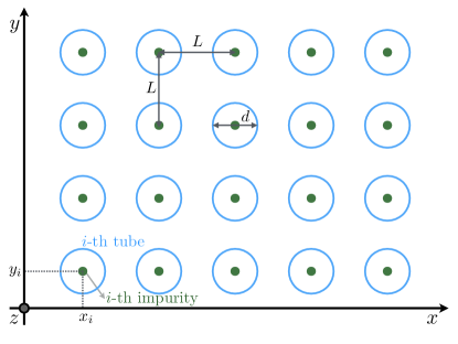
For the sake of clarity, let us first briefly call the working principle of the collisional sensor, which is schematically shown in Fig. 1. We consider an ensemble of noninteracting atoms (red wave packets on the left-hand side of the upper panel). Each atom is injected into its corresponding quasi-one dimensional waveguide (blue cylinders). Such a setup can be experimentally realized by means of a deep three-dimensional (3D) optical lattice with single-site access, which is then relaxed in the longitudinal direction in a controlled way so that each atom acquires a longitudinal momentum (see, e.g. Refs. Meinert et al. (2017); Robens et al. (2017)). In the centre of each waveguide there is a tightly confined atom (green spheres), either of the same species or of a different one with respect to the moving atoms. The collision can lead to transmission or reflection of the incoming atoms by the impurity. Transmitted (and possibly also reflected) atoms are then detected. The sensitivity of the measurement on the magnetic field is due to a Feshbach resonance that controls the interaction strength between the atom and the impurity. It is possible to tune the parameters in such a way that the probability of reflecting the colliding atom back from the impurity strongly depends on the local value of the magnetic field. The spatial spread of the waveguides (see lower panel in Fig. 1) allows us to gather information about the average magnetic field strength at their positions, therefore providing information about the field gradient.
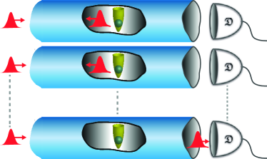
The paper is structured as follows: In Sec. II we describe atomic scattering in a quasi-1D waveguide in the vicinity of a Feshbach resonance. In Sec. III we analyse the sensor performance by providing experimentally relevant examples as well. Conclusions are drawn in Sec. IV, whereas in the appendix we review briefly multiparameter estimation theory.
II Atomic scattering in a quasi-1D waveguide
The problem of cold atomic scattering in quasi-one-dimensional confinement has been extensively studied in the literature Olshanii (1998); Bergeman et al. (2003); Granger and Blume (2004); Kim et al. (2006); Naidon et al. (2007); Giannakeas et al. (2012, 2013); Peng et al. (2014); Heß et al. (2014); Idziaszek et al. (2015); Heß et al. (2015); Melezhik and Negretti (2016); Jachymski et al. (2017). Here, we only provide a brief review of the most relevant results.
Assuming that the impurity atom is pinned in space (see Supplementary Material of Ref. Jachymski et al. (2018) for a discussion of this assumption), the problem can be described with the stationary Schrödinger equation for the motion of the incoming confined atom [here ]:
| (1) |
Here, is the mass of the atom, is the transverse harmonic trapping potential [with and its characteristic length ], and is the potential resulting from the interaction with the impurity.
At large distances, the interaction vanishes and the wavefunction can be decomposed into the initial harmonic oscillator mode in the transverse direction and even and odd plane waves in the longitudinal direction. In the general case, inelastic scattering can occur and lead to finite population of modes. In the following, we restrict our considerations to the lowest mode of the transverse oscillator, which should provide the best conditions for precise measurements. Extension of the calculations to higher modes is straightforward, albeit tedious. The total energy of the incoming atom can then be given as a sum of the harmonic and unconfined part
| (2) |
and is conserved during the collision, as the impurity is tightly trapped and cannot change its state. Note that we distinguish here the three-dimensional momentum from the one-dimensional .
The scattering can be completely described in terms of two scattering amplitudes, which are related to the one-dimensional phase shifts by:
| (3) |
In the case of identical bosons, symmetry allows only the even scattering. However, we are interested in the case of distinguishable particles, and thus we keep the odd term for the sake of generality. The transmission coefficient, which describes the part of the flux that goes through the waveguide, can then be defined as Olshanii (1998):
| (4) |
This expression can be conveniently rewritten in terms of the phase shift as .
We now need to connect the one-dimensional phase shifts to three-dimensional scattering quantities. This can be done analytically if the length scale characterizing the interaction range is much smaller than the trap width . One can then describe the scattering by a zero-range pseudopotential Olshanii (1998); Bergeman et al. (2003) or equivalently use frame transformation techniques Granger and Blume (2004). In general, even partial waves contribute only to the even part of the one-dimensional scattering, while odd partial waves describe the odd part. Restriction to the -wave () interaction results in Olshanii (1998)
| (5) |
Here, is the 3D energy-dependent scattering length that is rescaled by the factor due to our assumption of a pinned scattering center, and with being the Hurwitz zeta function.
Higher partial waves can be especially important for long-range interactions at low energies due to the different threshold laws. For -wave interactions, one obtains the following contribution to the odd phase shift Granger and Blume (2004)
| (6) |
where is the 3D -wave scattering volume.
Inclusion of the -wave in the potential modifies the even part of the scattering as Giannakeas et al. (2012):
| (7) |
Here, is the 3D -wave scattering length, and are again given by Hurwitz zeta functions. Note that in all the above formulas the scattering lengths are calculated at finite , corresponding to the total energy of the atom including the transverse confinement.
Analytical formulas can be derived for arbitrary partial waves Heß et al. (2015). In general, higher partial waves lead to emergence of additional very narrow resonances. These occur when their respective scattering lengths become comparable with the trap width, similarly to the -wave case. In the presence of a magnetic Feshbach resonance, all the scattering lengths corresponding to a partial wave can be tuned. The -wave scattering length in the zero energy limit close to the Feshbach resonance is described by the universal formula Chin et al. (2010)
| (8) |
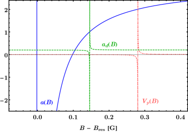
with being the resonance width, its position and the scattering length away from the resonance. Scattering in higher partial waves depends on the details of the interaction potential. Here, we choose the interaction to have the van der Waals form with characteristic length , as defined in Ref. Gribakin and Flambaum (1993), and being the Euler gamma function. This interaction is typical for the scattering of ultracold neutral atoms. We numerically solve the three-dimensional scattering problem with this potential in the presence of a Feshbach resonance and obtain the scattering phase shifts in Eqs. (5)-(7) as a function of the magnetic field. We note that the analytic theory developed by Gao Gao (1998, 2000) predicts that the -wave scattering volume diverges, as a function of the magnetic field , exactly at , and the -wave scattering length at . Figure 2 shows the magnetic field dependence of the scattering lengths for an exemplary Feshbach resonance characterized by the width G. The higher partial wave resonances occur exactly where expected.
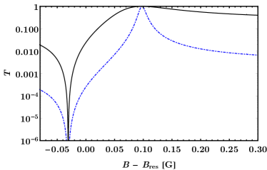
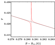
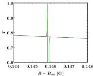
Having calculated the 3D scattering lengths, we can exploit Eqs. (4)–(7) to compute the transmission coefficient as a function of the magnetic field. The results are presented in Fig. 3. The insets show the narrow resonances resulting from the contribution of higher partial waves. Away from these resonances, the transmission is well described by the simple model which includes only the -wave scattering.
While in the above calculation we assumed that the impurity is pinned in the center of the waveguide, this approximation can be relaxed. The motion of the impurity in a tight trap, even displaced from the center, can be included and will result in slight shift of the resonance positions as well as emergence of multiple narrow confinement induced resonances due to coupling of the center of mass and relative motion Massignan and Castin (2006).
III Sensor performance
The transmission of the atoms through the waveguides is strongly affected by the proximity of the scattering resonances. This phenomenon was used in Ref. Jachymski et al. (2018) to estimate the value of the magnetic field by exploiting a single waveguide. Below, we investigate the possibility of measuring the strength of the magnetic field and, simultaneously, its spatial gradient utilizing an array of parallel waveguides (see also Fig. 1).
To begin with, we will first perform a simple analysis of the precision achievable using an isolated single tube. Then, we apply the multiparameter estimation formalism discussed in the appendix to fully characterize the precision of the sensor for both the field value and of its gradient components.
III.1 Field strength estimation with a single tube
In this scenario, the probability of detecting a transmitted or reflected atom is only sensitive to the strength of the magnetic field. In such a single-parameter estimation problem, the lower bound on the variance of an unknown parameter is provided by the so-called classical Cramér-Rao theorem Braunstein and Caves (1994); Réfrégier (2012); Cramér (2016). Accordingly, the ultimate attainable uncertainty of the estimated field at large atom numbers is given by
| (9) |
where denotes the number of injected atoms into the tube (red wave packets in Fig. 1). The scaling is a statistical factor coming from the increase of independent resources. The figure of merit of the sensor is given by the Fisher information Réfrégier (2012) that is defined as
| (10) |
Here, is the transmission probability, and is the probability of reflecting the atom in the collision with the impurity. The precision bound given by Eq. (9) is saturated asymptotically by the maximum likelihood estimator in the limit of a large number of atoms used in the estimation procedure.
Expressing the probability distributions in terms of the transmission coefficient, , the Fisher information takes the following form:
| (11) |
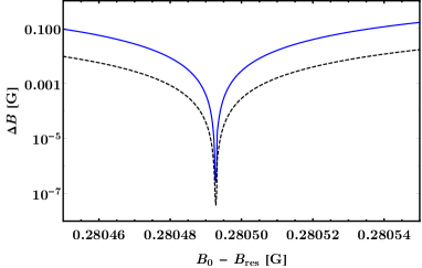
The formula (11) implies that the lowest uncertainty is attained when the derivative of the transmission coefficient is the largest. The behaviour of in the vicinity of and is determined by the dependence of close to these points. The case of the -wave resonance was analyzed in Ref. Jachymski et al. (2018). The uncertainty of the magnetic field in the vicinity of the -wave confinement-induced resonance as a function of is displayed in Fig. 4 for and two momenta: (dashed black line) and (solid blue line). One can notice that the uncertainty for the larger momentum is smaller. This is intuitively explained by the fact the probability of detecting a particle without reflection is increasing with momentum, but it rapidly drops to near zero value at the position of the confinement-induced resonance. The derivative of is larger if the change in transmission is bigger, which results in higher precision. With the -wave interactions only, for the chosen parameters the achievable uncertainty is of the order of G Jachymski et al. (2018), whereas at the -wave confinement-induced resonance we obtain G. Such a big increase in precision is related to the fact that the -wave resonance is much narrower than the -wave. However, the offset magnetic field has to be precisely controlled to ensure the atoms are close to the resonances in higher-partial waves. The results in Fig. 4 are improved further by a statistical factor of , if waveguides are used with atoms per waveguide, as in Fig. 1. Finally, we note that the above outlined observations and conclusions for the -wave resonance apply to the -wave resonance as well.
III.2 Performance of the magnetic gradiometer
We assume now that tubes are placed at fixed positions and that the magnetic field strength varies smoothly in space. In analogy to a single waveguide, we assign to the variable the value if the atom is transmitted through the waveguide and detected with (conditional) probability , and the value if the atom is reflected after the collision with the impurity. For waveguides, we define a new random variable . Thus, the probability of transmitting or reflecting an atom is
| (12) |
Here is the position of the impurity in the -th tube, and is the corresponding magnetic field strength. Then, we expand the field strength up to the first order, i.e. . Furthermore, we assume that all impurities are distributed on a plane, for which we set (see also lower panel of Fig. 1). Hence, we have
| (13) |
where and denote the and magnetic field gradient components, respectively, while and are the corresponding coordinates in the plane. Thus, the parameters that we aim at estimating from the measurement records of the atom transmission and reflection are the magnetic field strength , and its gradient components and .
In order to apply the general formalism described in the appendix, we rename the three () unknown parameters as follows: , , and . Because of the additivity of the Fisher information matrix with respect to independent events, the FIM can be rewritten as a sum of Fisher information matrices describing each waveguide separately:
| (14) |
By denoting and its derivative with respect to by , the -th FIM takes the form of a product of a factor depending on the transmission coefficient by a matrix describing the geometry of the problem, i.e., depending only on the positions of the waveguides:
| (15) |
Hence, by performing the sum from Eq. (14) with the above outlined expression for , we obtain the full Fisher information matrix for tubes, which, according to Eq. (19), provides us the minimal attainable uncertainty for each of the three unknown parameters , and . Let us remark that at least three non planar tubes are necessary in order to obtain a meaningful estimation of the gradient in two spatial directions. Indeed, mathematically, the structure of the matrix enforces the determinant of in Eq. (14) to vanish unless . Moreover, we note that the matrix is not invertible for planar tubes.
In order to analyze the performance of the sensor, we consider exemplarily the case of tubes with equal spacing nm in each direction (see lower panel in Fig. 1). For the sake of numerical simplicity, we assume that the field can change only along the direction, i.e., . Notwithstanding, the additional rows of the tubes array (see lower panel in Fig. 1) contribute statistically due to the accumulated data. Hence, in order to determine the minimal uncertainty, expressed by Eq. (19), of the magnetic field strength and its spatial derivative along the -axis, we can safely neglect in Eq. (15) the third column and the third row.
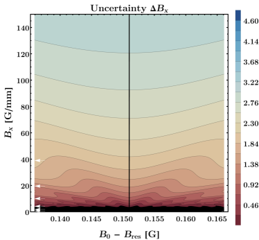
In Fig. 5 we display the attainable uncertainty in the estimation of the magnetic field strengh measured with respect to the resonance position . The parameters used in the calculation were G, , (similar to caesium atoms) and . For such a small momentum the optimal working point is expected near the unit transmission region , in contrast to the higher energy case, where the zero transmission region is favorable Jachymski et al. (2018). As it can be seen from the figure, the uncertainty depends on both parameters and . For vanishing gradient, the uncertainty changes appreciably around the optimal operating point , where is the resonance width, at which the transmission rapidly approaches unity (see also Fig. 3). At that point, the attainable uncertainty is on the order of G, which is further enhanced by the statistical factor related to the number of atoms used in the protocol. For the values of the field for which the transmission drops off by two orders of magnitude, the uncertainty deteriorates as well and reaches at best the order of G.
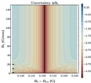
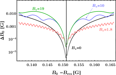
On the other hand, for a non-vanishing gradient, the uncertainty decreases by an order of magnitude, but it is maintained at the level of G for fields around and gradients up to few tens of Gauss per millimetre. Departure from for any value of the gradient leads to the increase of the uncertainty . In addition to this, as it can be seen from the Fig. 5 (lower panel), the precision exhibits wavy features as a function of when departing from the region near to . Furthermore, the “frequency” of this oscillatory behaviour is decreasing as the gradient increases. This phenomenon can be understood as follows: Let us first suppose that the gradient is zero and the sensor is working around its optimal operating point, namely . In this case, all the terms of the sum in Eq. (14) are of the same order and contribute a small uncertainty. However, when the gradient is small but non-zero, the local field at some of the waveguides is far from their optimal points, which decreases some terms in Eq. (14), and, consequently, the uncertainty of estimation grows. As the field strength is varied, the local field at some of the waveguides approaches the optimal points, while at other waveguides the local field is away from them. As a consequence, with the change of , the uncertainty is in general higher than the one at the optimal point, but it exhibits periodic increases and decreases, i.e. revivals. The same reasoning applies to (see Fig. 6).
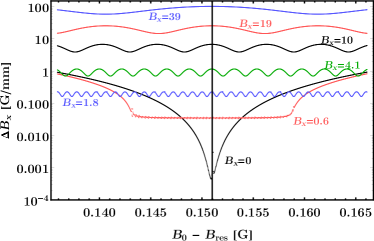
As it can be seen from Figs. 5 and 6, the “period” of such wavy features is larger for larger gradients. This can be understood in the following way: For small gradients, the local field at the waveguides is very close to their optimal points, and thus the period should be small. Instead, for large gradients, the local field is almost in all waveguides away from the optimal point and thus their contribution to the sum in Eq. (14) is small, implying a small uncertainty. Hence, the local field at a small number of waveguides will be near the optimal operating points as the field is varied, implying a larger period.
Finally, in Fig. 6, we present the minimal attainable uncertainty for the estimation of the magnetic field gradient along the direction. Similar to , the optimal operating point is achieved when and . However, contrary to the estimation of the field, departure from leads to an increase of the gradient uncertainty. Therefore, in this case, the performance of the sensor is the highest only for small gradients. For the parameters and geometry we have chosen, the uncertainty is the smallest and reaches the value for and small gradients. For increasing gradients, the precision deteriorates and for it is on the order of a Gauss per millimetre. We remind, however, that the uncertainties or presented so far are without the statistical factor , which is inherent in the statistical post-processing of the data and is related to finite resources used during the estimation procedure. By multiplying those uncertainties with that numerical factor, we can further improve the sensitivity of the proposed sensor. Thus, also for increasing gradients, repeated measurements can improve the performance of the proposed gradiometer also away from the optimal operating point. Finally, similarly to and for the same reason discussed above, we observe that the precision exhibits an oscillatory behaviour as a function of the magnetic field (see Fig. 6 lower panel).
IV Summary and conclusions
We have proposed a new magnetic field sensor scheme utilizing atomic collisions in an array of waveguides. At the input of the device, single atoms are injected into the waveguides, and then collide with the impurities, while the transmitted and reflected atoms are detected at the end of each waveguide. From such a measurement recording, we infer the values of the characteristic properties of the external magnetic field, that is, the strength of the field and its gradient along two directions.
We provided the attainable values of the uncertainties of the field characteristics. In our previous work Jachymski et al. (2018), we proposed a sensor operating only on a single waveguide and we showed that it is possible to reach an uncertainty of the field strength of the order of nT/. Here, we extended the concept and showed that the multi-waveguide configuration of the sensor can be exploited to simultaneously measure magnetic field strength and its gradient with a precision on the order of 1 nT/ and 100 nT/(mm ), respectively.
The achievable precision can be still improved by a number of strategies. First, the simplest way to reduce the uncertainty is by increasing the number of atoms at the input, which improves the statistical scaling of the uncertainty. Second, the possibility to tune the system (e.g., by controlling the frequency of the transverse trap) into the vicinity of the scattering resonances in the higher partial waves can decrease the uncertainty of the magnetic field by a few orders of magnitude. Such an approach, however, is experimentally demanding since the offset field has to be precisely controlled. We note that long-range interactions between atoms and the impurity will also generate additional narrow resonances, which might be employed for metrology leading to a similar sensor’s performance as in the case of resonances in higher partial waves. Lastly, the use of initial entangled states can in principle lead to a further decrease of the uncertainty due to quantum correlations in a similar manner as squeezed or GHZ states employed in photonic quantum metrology Giovannetti et al. (2006). For this last strategy, however, one needs to devise experimentally feasible protocols for engineering entangled input states and collective measurements.
To conclude, our work demonstrates that ultracold atomic collisions are useful for quantum sensing. Since Feshbach resonances can be controlled by many techniques, the device we propose can find various applications in ultracold laboratories, where the magnetic field and its spatial characteristics have to be precisely known, e.g., in quantum simulators based on atoms in optical lattices Gross and Bloch (2017). In the current state, the sensor operates in a limited magnetic field range close to the Feshbach resonance and as such requires calibration with respect to the resonance position. It would be desirable to get rid of this requirement, possibly providing a more universal metrological standard in the future.
Acknowledgements.
We are grateful to Paul S. Julienne and Zbigniew Idziaszek for valuable discussions. This work was supported by the Alexander von Humboldt Foundation, the Polish National Science Center Project No. 2014/14/M/ST2/00015, the Cluster of Excellence The Hamburg Centre for Ultrafast Imaging of the Deutsche Forschungsgemeinschaft, and the European Union FP7 FET Proactive Project DIADEMS (Grant No. 611143).Appendix A Multiparameter estimation formalism
Here we describe the general formalism used in the main text in order to make use of the multiparameter estimation Helstrom (1976).
To begin with, let us denote the vector containing unknown parameters to be estimated by . Specifically to our problem, the parameter is the strength of the magnetic field at some arbitrary point in space, whereas and are the and components of the field gradient (cf. Fig. 1); this is an estimation of unknown parameters.
The parameters have to be extracted from the measurement record of a certain experimentally accessible observable . In our setting, denotes a reading of the detectors situated at the end of each of the waveguides, yielding the number of transmitted atoms. More specifically, if an atom is recorded at the -th waveguide, the component of is assigned a prescribed value, taken arbitrarily equal to, say, .
After of such independent experimental runs, a data set is obtained, where denotes an outcome of the -th experimental run of the observable . The probability of obtaining in an experimental run is given by , i.e., it is conditioned on the actual value, yet unknown, of the parameters to be determined. Thus, the outcomes of the runs of the experiment, assuming statistical independence, are governed by a joint probability distribution . Hence, the distribution of the observed outcomes is governed by the underlying values of the parameters , too. The inference about the value of the unknown parameter vector is drawn from the data by means of a certain function of the acquired measurement data. The function is generally called the estimator and yields an estimate of the unknown parameters, i.e., it is expected that . Since the outcomes of the measurements fluctuate from run to run, the estimation of the unknown parameters is always accompanied by an uncertainty. As an example of an estimator, the maximum likelihood estimator is defined as the value of that maximizes .
The performance of a multiparameter estimation is conveniently represented by a covariance matrix , whose matrix elements are given by
| (16) | |||||
Here the average in the first line is taken over the joint distribution and the sum over in the second line is taken over all possible values of the outcomes of . For an unbiased estimator, the mean value of , taken over the probability distribution , is equal to the true value of the unknown parameter vector . In this case, the covariance matrix satisfies the inequality
| (17) |
which is known as the Cramér-Rao theorem Helstrom (1976); Réfrégier (2012) and it has to be understood in the matrix sense, i.e. is a positive semi-definite matrix. The inequality (17) provides a (lower) bound for the performance of the multiparameter estimation and it is expressed in terms of the inverse of the Fisher information matrix (FIM) , whose elements are given by:
| (18) |
The FIM depends only on the probability distribution from which is constructed. The information about is inherited in the statistical prefactor , which ensures that smaller uncertainties can be attained when larger data sets are used for estimation.
In this work, we quantify the uncertainty of the unknown parameter by the variance of the estimator for each of the corresponding estimated parameters, i.e., . The Cramér-Rao theorem states that such variances are bounded by the inverse of the Fisher information matrix Réfrégier (2012). The bounds, which represent the minimal uncertainty that can be attained in the estimation of the parameters, take the form
| (19) |
These bounds are saturated asymptotically in , in the limit of very large samples, by the maximum likelihood estimator Helstrom (1976); Réfrégier (2012). We note, however, that in practice the estimated uncertainties will be larger than the above outlined bounds.
References
- Bloom et al. (2014) B. Bloom, T. Nicholson, J. Williams, et al., Nature 506, 71 (2014).
- Nicholson et al. (2015) T. Nicholson, S. Campbell, R. Hutson, G. Marti, B. Bloom, R. McNally, W. Zhang, M. Barrett, M. Safronova, G. Strouse, et al., Nature Communications 6 (2015).
- Hoover et al. (1996) D. B. Hoover, D. P. Klein, and D. C. Campbell, Report No. 95-831 , U.S. Geological Survey (1996).
- DeGregoria (2010) A. DeGregoria, Ph.D. thesis (Air Force Institute of Technology, 2010).
- Sander et al. (2012) T. Sander, J. Preusser, R. Mhaskar, J. Kitching, L. Trahms, and S. Knappe, Biomed. Opt. Express 3, 981 (2012).
- Jensen et al. (2016) K. Jensen, R. Budvytyte, R. A. Thomas, T. Wang, A. M. Fuchs, M. V. Balabas, G. Vasilakis, L. D. Mosgaard, H. C. Stærkind, J. H. Müller, T. Heimburg, S.-P. Olesen, and E. S. Polzik, Sci. Rep. 6, 29638 (2016).
- Balasubramanian et al. (2008) G. Balasubramanian, I. Chan, R. Kolesov, M. Al-Hmoud, J. Tisler, C. Shin, C. Kim, A. Wojcik, P. R. Hemmer, A. Krueger, et al., Nature 455, 648 (2008).
- Chen et al. (2006) J. L. Chen, C. R. Wilson, and B. D. Tapley, Science 313, 1958 (2006).
- Webb et al. (1999) J. K. Webb, V. V. Flambaum, C. W. Churchill, M. J. Drinkwater, and J. D. Barrow, Phys. Rev. Lett. 82, 884 (1999).
- Chin and Flambaum (2006) C. Chin and V. V. Flambaum, Phys. Rev. Lett. 96, 230801 (2006).
- Zelevinsky et al. (2008) T. Zelevinsky, S. Kotochigova, and J. Ye, Phys. Rev. Lett. 100, 043201 (2008).
- Blatt et al. (2008) S. Blatt, A. Ludlow, G. Campbell, J. W. Thomsen, T. Zelevinsky, M. Boyd, J. Ye, X. Baillard, M. Fouché, R. Le Targat, et al., Phys. Rev. Lett. 100, 140801 (2008).
- Hudson et al. (2011) J. J. Hudson, D. M. Kara, I. Smallman, B. E. Sauer, M. R. Tarbutt, and E. A. Hinds, Nature 473, 493 (2011).
- Baron et al. (2014) J. Baron, W. C. Campbell, D. DeMille, J. M. Doyle, G. Gabrielse, Y. V. Gurevich, P. W. Hess, N. R. Hutzler, E. Kirilov, I. Kozyryev, et al., Science 343, 269 (2014).
- Schnabel et al. (2010) R. Schnabel, N. Mavalvala, D. E. McClelland, and P. K. Lam, Nat. Comm. 1, 121 (2010).
- Schlippert et al. (2014) D. Schlippert, J. Hartwig, H. Albers, L. L. Richardson, C. Schubert, A. Roura, W. P. Schleich, W. Ertmer, and E. M. Rasel, Phys. Rev. Lett. 112, 203002 (2014).
- Biedermann et al. (2015) G. W. Biedermann, X. Wu, L. Deslauriers, S. Roy, C. Mahadeswaraswamy, and M. A. Kasevich, Phys. Rev. A 91, 033629 (2015).
- Rosi et al. (2017) G. Rosi, G. D’Amico, L. Cacciapuoti, F. Sorrentino, M. Prevedelli, M. Zych, Č. Brukner, and G. M. Tino, Nat. Comm. 8, 15529 (2017).
- Ferrari et al. (2006) G. Ferrari, N. Poli, F. Sorrentino, and G. M. Tino, Phys. Rev. Lett. 97, 060402 (2006).
- Salumbides et al. (2013) E. J. Salumbides, J. C. J. Koelemeij, J. Komasa, K. Pachucki, K. S. E. Eikema, and W. Ubachs, Phys. Rev. D 87, 112008 (2013).
- Borkowski et al. (2017) M. Borkowski, A. Buchachenko, R. Ciuryło, P. Julienne, H. Yamada, K. Yuu, K. Takahashi, Y. Takasu, and Y. Takahashi, in Journal of Physics: Conference Series, Vol. 810 (IOP Publishing, 2017) p. 012014.
- Giovannetti et al. (2004) V. Giovannetti, S. Lloyd, and L. Maccone, Science 306, 1330 (2004).
- Giovannetti et al. (2006) V. Giovannetti, S. Lloyd, and L. Maccone, Phys. Rev. Lett. 96, 010401 (2006).
- Petersen et al. (2005) V. Petersen, L. B. Madsen, and K. Mølmer, Phys. Rev. A 71, 012312 (2005).
- Petersen and Mølmer (2006) V. Petersen and K. Mølmer, Phys. Rev. A 74, 043802 (2006).
- Chase and Geremia (2009) B. A. Chase and J. M. Geremia, Phys. Rev. A 79, 022314 (2009).
- Chase et al. (2009) B. A. Chase, B. Q. Baragiola, H. L. Partner, B. D. Black, and J. M. Geremia, Phys. Rev. A 79, 062107 (2009).
- Negretti and Mølmer (2013) A. Negretti and K. Mølmer, New Journal of Physics 15, 125002 (2013).
- Martin Ciurana et al. (2017) F. Martin Ciurana, G. Colangelo, L. Slodička, R. J. Sewell, and M. W. Mitchell, Phys. Rev. Lett. 119, 043603 (2017).
- Fernholz et al. (2008) T. Fernholz, H. Krauter, K. Jensen, J. F. Sherson, A. S. Sørensen, and E. S. Polzik, Phys. Rev. Lett. 101, 073601 (2008).
- Wasilewski et al. (2010) W. Wasilewski, K. Jensen, H. Krauter, J. J. Renema, M. V. Balabas, and E. S. Polzik, Phys. Rev. Lett. 104, 133601 (2010).
- Riedel et al. (2010) M. F. Riedel, P. Böhi, Y. Li, T. W. Hänsch, A. Sinatra, and P. Treutlein, Nature 464, 1170 (2010).
- Krischek et al. (2011) R. Krischek, C. Schwemmer, W. Wieczorek, H. Weinfurter, P. Hyllus, L. Pezzé, and A. Smerzi, Phys. Rev. Lett. 107, 080504 (2011).
- Hardman et al. (2016) K. S. Hardman, P. J. Everitt, G. D. McDonald, P. Manju, P. B. Wigley, M. A. Sooriyabandara, C. C. N. Kuhn, J. E. Debs, J. D. Close, and N. P. Robins, Phys. Rev. Lett. 117, 138501 (2016).
- Kruse et al. (2016) I. Kruse, K. Lange, J. Peise, B. Lücke, L. Pezzè, J. Arlt, W. Ertmer, C. Lisdat, L. Santos, A. Smerzi, and C. Klempt, Phys. Rev. Lett. 117, 143004 (2016).
- Jachymski et al. (2018) K. Jachymski, T. Wasak, Z. Idziaszek, P. S. Julienne, A. Negretti, and T. Calarco, Phys. Rev. Lett. 120, 013401 (2018).
- Meinert et al. (2017) F. Meinert, M. Knap, E. Kirilov, K. Jag-Lauber, M. B. Zvonarev, E. Demler, and H.-C. Nägerl, Science 356, 945 (2017).
- Robens et al. (2017) C. Robens, J. Zopes, W. Alt, S. Brakhane, D. Meschede, and A. Alberti, Phys. Rev. Lett. 118, 065302 (2017).
- Olshanii (1998) M. Olshanii, Phys. Rev. Lett. 81, 938 (1998).
- Bergeman et al. (2003) T. Bergeman, M. Moore, and M. Olshanii, Phys. Rev. Lett. 91, 163201 (2003).
- Granger and Blume (2004) B. E. Granger and D. Blume, Phys. Rev. Lett. 92, 133202 (2004).
- Kim et al. (2006) J. I. Kim, V. S. Melezhik, and P. Schmelcher, Phys. Rev. Lett. 97, 193203 (2006).
- Naidon et al. (2007) P. Naidon, E. Tiesinga, W. F. Mitchell, and P. S. Julienne, New Journal of Physics 9, 19 (2007).
- Giannakeas et al. (2012) P. Giannakeas, F. K. Diakonos, and P. Schmelcher, Phys. Rev. A 86, 042703 (2012).
- Giannakeas et al. (2013) P. Giannakeas, V. S. Melezhik, and P. Schmelcher, Phys. Rev. Lett. 111, 183201 (2013).
- Peng et al. (2014) S.-G. Peng, S. Tan, and K. Jiang, Phys. Rev. Lett. 112, 250401 (2014).
- Heß et al. (2014) B. Heß, P. Giannakeas, and P. Schmelcher, Phys. Rev. A 89, 052716 (2014).
- Idziaszek et al. (2015) Z. Idziaszek, K. Jachymski, and P. S. Julienne, New Journal of Physics 17, 035007 (2015).
- Heß et al. (2015) B. Heß, P. Giannakeas, and P. Schmelcher, Phys. Rev. A 92, 022706 (2015).
- Melezhik and Negretti (2016) V. S. Melezhik and A. Negretti, Phys. Rev. A 94, 022704 (2016).
- Jachymski et al. (2017) K. Jachymski, F. Meinert, H. Veksler, P. S. Julienne, and S. Fishman, Phys. Rev. A 95, 052703 (2017).
- Chin et al. (2010) C. Chin, R. Grimm, P. Julienne, and E. Tiesinga, Rev. Mod. Phys. 82, 1225 (2010).
- Gribakin and Flambaum (1993) G. F. Gribakin and V. V. Flambaum, Phys. Rev. A 48, 546 (1993).
- Gao (1998) B. Gao, Phys. Rev. A 58, 1728 (1998).
- Gao (2000) B. Gao, Phys. Rev. A 62, 050702 (2000).
- Massignan and Castin (2006) P. Massignan and Y. Castin, Phys. Rev. A 74, 013616 (2006).
- Braunstein and Caves (1994) S. L. Braunstein and C. M. Caves, Phys. Rev. Lett. 72, 3439 (1994).
- Réfrégier (2012) P. Réfrégier, Noise theory and application to physics: from fluctuations to information (Springer Science & Business Media, 2012).
- Cramér (2016) H. Cramér, Mathematical Methods of Statistics (PMS-9), Vol. 9 (Princeton university press, 2016).
- Gross and Bloch (2017) C. Gross and I. Bloch, Science 357, 996 (2017).
- Helstrom (1976) C. W. Helstrom, Quantum detection and estimation theory (Academic Press, 1976).