Accelerating a Landscape Evolution Model with Parallelism

Abstract

Solving inverse problems and achieving statistical rigour in landscape evolution models requires running many model realizations. Parallel computation is necessary to achieve this in a reasonable time. However, no previous algorithm is well-suited to leveraging modern parallelism. Here, I describe an algorithm that can utilize the parallel potential of GPUs, many-core processors, and SIMD instructions, in addition to working well in serial. The new algorithm runs 43 x faster (70 s vs. 3,000 s on a 10,000 x 10,000 input) than the previous state of the art and exhibits sublinear scaling with input size. I also identify methods for using multidirectional flow routing and quickly eliminating landscape depressions and local minima. Tips for parallelization and a step-by-step guide to achieving it are given to help others achieve good performance with their own code. Complete, well-commented, easily adaptable source code for all versions of the algorithm is available as a supplement and on Github.

1 Software Availability

Complete, well-commented, easily-adaptable source code, an associated makefile, and correctness tests are available at https://github.com/r-barnes/Barnes2018-Landscape. The code is written in C++ using OpenACC for GPU acceleration and OpenMP for multi-core CPU acceleration. The code constitutes 3,304 lines of code spread across several implementations (averaging 367 lines of code per implementation) of which 42% are or contain comments.

2 Introduction

Models can be used to determine how landscapes are formed and to predict their future. However, doing so requires choosing between many possible governing equations [25, 7] and initial conditions. The analyses necessary to judge between the options require millions of model realizations and, to achieve statistical rigor, many thousands more. [5, 25] This computational cost is exacerbated by need for numerical stability and accuracy, which often requires using small time increments and high spatial resolutions. If is not feasible to perform these runs in serial. The algorithms I present below will enable landscape evolution researchers to achieve statistical rigor with minimal difficulty and computational cost.

Making use of SIMD, GPUs, and other accelerators will become increasingly important in the future. CPU clock-speeds are no longer increasing and, in some cases, are deliberately decreased to promote energy-efficiency. At the same time, core counts and data parallel architectures are becoming common. The algorithm and implementations I present here are better suited to this emerging paradigm than previous landscape evolution models.

The most efficient algorithm previously published is an $O(n)$ implicit integrator developed by Braun and Willett [5]. I will refer to this below as the B&W algorithm and use it to benchmark the performance of the new code.

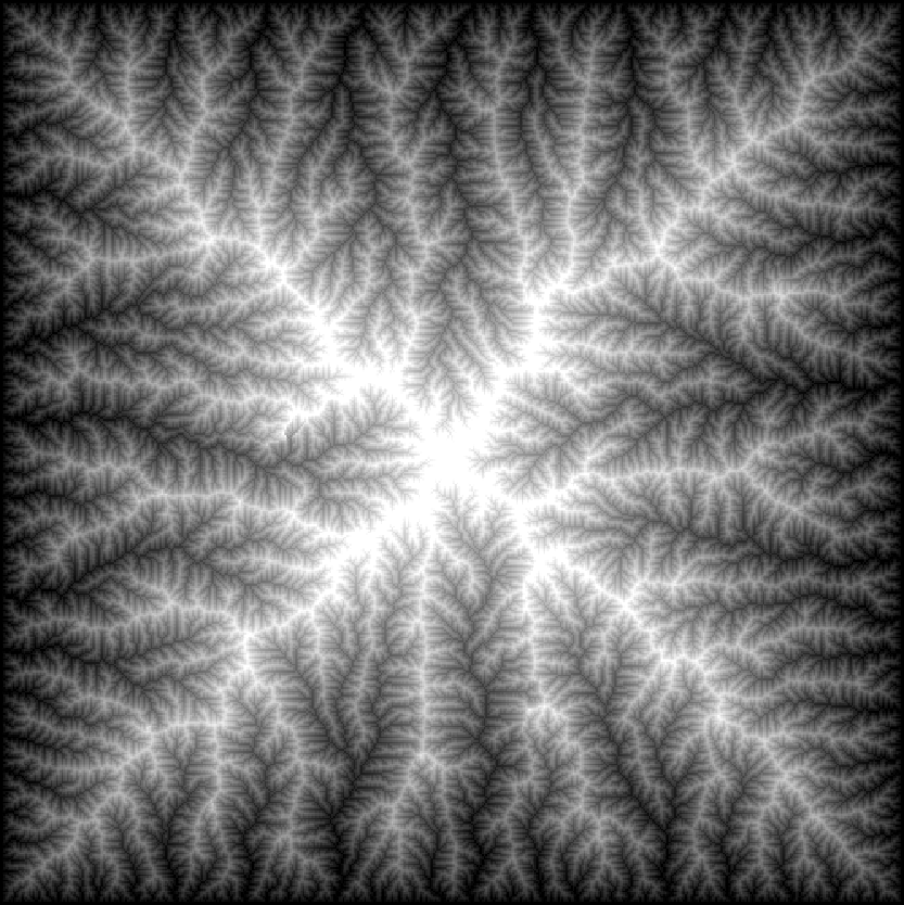
Figure 1: An example output of the landscape evolution algorithm.

The design of the B&W algorithm imposes serious limitations on parallelism and scalability; it is also limited to D8 flow routing. In contrast, my new algorithm can fully leverage SIMD (single instruction, multiple data) instructions such as the SSE and AVX families within a single core, distribute work without load imbalance between many cores, effectively offload work to accelerators such as GPUs, and work with multiple-flow direction routing. The algorithm produces outputs similar to that shown in Figure 1.

3 The Equation

Though the algorithm described here could be applied to many equations governing the evolution of landscapes ([25, 7] offer reviews), in this paper I use the stream power equation as an example as it has been widely used in the field. [11, 20, 27] In the equation, the evolution of the elevation $h$ of a point on a landscape is modeled as:

$$\frac{\partial h}{\partial t}=-KA^{\hat{m}}\left(\frac{\partial h}{\partial x}\right)^{\hat{n}}$$ (1)

where $K$ is a scalar influenced by lithology, channel width, and channel hydrology, among other possibilities; $A$ is the flow accumulation or contributing drainage area; and $\hat{m}$ and $\hat{n}$ are scaling constants. The implicit (backwards) Euler method using Newton-Raphson for the nonlinearity may be used to this equation. [5].

Equation 1 must be solved for all of the cells in an DEM. This requires a boundary condition (here I set the DEM’s perimeter cells to a fixed base level, Braun and Willett [5] discusses other possibilities), the flow accumulation and slope at each point, and an ordering of points such that those receiving flow from a higher neighbour are processed before that neighbour. Below, I describe how to obtain these elements in a parallelized way.

4 On Parallelism

The following are a few notes on parallelism that guide algorithm design. The pseudocode in this paper instantiates these details at the conceptual level, but, since parallelism is maddeningly difficult [13] to get right, the reader is advised to refer to the provided implementations for full details.

4.1 Amdahl’s law

Amdahl’s law says that a program’s speed-up due to parallelism is bounded by the number of available parallel units and the time the program must spend running serial code; any serial code acts as a bottleneck. In B&W only a subset of the steps of the algorithm are parallelized; therefore, as the number of parallel units increases, the run-time is dominated by the serial steps. Here, I overcome this by parallelizing all steps.

4.2 Parallel For

The algorithm consists of several distinct steps. Each step involves one or more loops over the elevation model, or portions thereof. These loops may be parallelized when their iterations are independent of each other. Such loops are denoted in the pseudocode with for_∥. For instance, during Uplift (§5.6, Algorithm 5.6) each cell is raised by a constant factor. Since no cell needs information from any other cell for this to happen, all the cells may be uplifted concurrently.

4.3 Concurrent Steps

Sometimes, one or more steps may be executed concurrently. For example, the Flow Accumulation subroutine (§5.5, Algorithm 5.5) does not depend on the elevations of the cells and the Uplift subroutine (§5.6, Algorithm 5.6) does not depend on flow accumulation. As a result, the two steps could be run at the same time.

4.4 Barriers and Synchronization

Both OpenMP and OpenACC—two widely-used interfaces for parallel programming—require that all threads synchronize at the end of each parallel for region; this is known as an implicit barrier. This prevents steps from being run concurrently. Eliminating barriers is vital to obtaining good parallel performance. In my implementations, I remove many implicit barriers, allowing threads to independently proceed through several steps before reaching a barrier. For simplicity the pseudocode does not show this, but readers can find full details in the reference implementation.

4.5 Simplified Flow Control

The presence of if clauses within the inner loops of an algorithm can lead to slow downs (by a factor of 2 or more) when the CPU fails to predict which value the if will take (failed branch prediction) or the GPU’s warps diverge. The mere existence of an if clause within a loop is often sufficient to prevent it from being vectorized for SIMD. To counter this, wherever possible, I try to keep the inner bodies of loops simple.

5 The Algorithm

Cell	1	2	3	4	5	6	7	8	9	10
Elev	3	2	3	4	1	2	3	2	4	3
Rec	2	5	2	7	X	5	6	5	7	8
Donor	-	1	-	-	2	7	4	10	-	-
	-	3	-	-	6	-	9	-	-	-
	-	-	-	-	8	-	-	-	-	-
Dnum	0	2	0	0	3	1	2	1	0	0
Queue	5	2	6	8	1	3	7	10	4	9
Levels	0	1	4	8	10
Accum	1	3	1	1	10	4	3	2	1	1

Table 1: Arrays used in the algorithm: a worked example. All arrays are zero-indexed. The entries of the Cell row refer to the node labels in Figure 2. Elevations are chosen arbitrarily such that donor cells are higher than receiver cells. Receivers are calculated per Algorithm 5.2. Donors are calculated per Algorithm 5.3. Note that the Donor array should be read as snaking down one column, then down the next, and so on. Each column refers to one node’s entries and each node has Dmax entries, some of which are unused (these are marked with dashes ‘-’). The Dnum array is the number of entries of each column of the Donor array which are filled in; that is, the number of Donors each cell has. The Queue array is the order in which cells should be processed, as determine by Algorithm 5.4; these values are the same as those shown in Figure 3b. The Levels array notes the 0-indexed beginnings of each level of parallelized cells, as marked by the dashed lines in Figure 3b. The flow Accumulation array shows the flow accumulation of each cell, as determined by Algorithm 5.5.

The algorithm models each grid cell as having receiver nodes (those receiving flow from an upslope neighbour) and donor nodes (those nodes which pass their flow to a downslope neighbour). Figure 2 depicts these concepts.

The algorithm assumes that a regular, 4-, 6-, or 8-connected grid is used. This is important since it provides a simple addressing mechanism for cells and enables the processor to intelligently prefetch data from RAM, which is slow, and maintain it in the L1, L2, and L3 caches, which are fast. [8, 22] It also permits efficient transfer of memory between the CPU and GPU.

Table 1 shows a worked example of the arrays developed in the following algorithms.

Figure 2: Elevation nodes and their connections. Solid arrows denote flow along the path of greatest slope while dashed lines denoted possible flow routes of lesser slope which are modeled as having no flow. In this example, Nodes 4 and 9 are the donors of Node 7 and Node 6 is the receiver of Node 7. Node 5 is at the base level (marked by the solid line) and its elevation does not change. Figure adapted from [5].

5.1 Step 1: Initialization

The algorithm requires several global variables. These are as follows:

• Dmax: The maximum number of potential donors of any cell in the elevation model. For a rectangular grid with horizontal, vertical, and diagonal connections, this is 8.

• $\hat{m}$: The exponent of the flow accumulation area in the stream power equation (Equ. 1).

• $\hat{n}$: The exponent of the local slope in the stream power equation (Equ. 1).

• $\hat{u}$: The rate of uplift.

• NoFlow: A constant indicating that the cell has no receiver.

• $\epsilon$: The tolerance for convergence in the Newton-Raphson method.

The algorithm requires one input array:

• Elev: The height/elevation model. This is a one-dimensional array of size width by height. A particular cell at location $(x,y)$ is addressed as $y\cdot\textit{width}+x$.

5.2 Step 2: Determine Receivers

Here, for each cell $c$, we determine which of $c$’s neighbours receives its flow, choosing the neighbour with the greatest downhill slope. The address of the receiving neighbour is stored in the Rec array. Each entry in this array has a corresponding cell in the Elev array. Note that cells on the perimeter of the model do not transfer flow.

  Algorithm 1 Determine Receivers

 

1:Let $Rec$ have the same dimensions as $Elev$

2:Initialize $Rec$ to NoFlow

3:

4:for_∥ all cells $c$ in the interior of $Elev$

5:    $s_{\textrm{max}}\leftarrow 0$ $\triangleright$ Maximum slope

6:    $n_{\textrm{max}}\leftarrow\textsc{NoFlow}$ $\triangleright$ Neighbour with that slope

7:    for all neighbours $n$ of $c$ do

8:        $s\leftarrow(Elev[c]-Elev[n])/\textrm{dist}(c,n)$

9:        $\triangleright$ Slope from $c$ to $n$

10:        if $s>s_{\textrm{max}}$ then

11:           $s_{\textrm{max}}\leftarrow s$

12:           $n_{\textrm{max}}\leftarrow n$             

13:    $Rec[c]\leftarrow n_{\textrm{max}}$

 

5.3 Step 3: Determine Donors

The Donors array is an inversion of the Rec array. Each cell in Elev corresponds to Dmax entries in this array, where each entry denotes the address of a cell from which flow is received. Thus, the address of the cells from which a particular cell $(x,y)$ will receive flow are given by $\textit{Dmax}\cdot(y\cdot\textit{width}+x)+k=\textit{Dmax}\cdot c+k$ for $k\in[0,\textit{Dnum}(c))$, where $\textit{Dnum}(c)$ indicates the number of neighbours from which $c$ receives flow.

In the B&W algorithm, each donating cell informs its receiver that it will be receiving a donation. This prevents parallelization because multiple donor cells may pass their information at the same time: a race condition. This could be prevented with atomic operations, but a more performant solution is to have each cell identify its donors.

  Algorithm 2 Determine donors

 

1:Let $Donor$ have the same dimensions as $Elev\cdot\textit{Dmax}$

2:Let Dnum have the same dimensions as $Elev$

3:

4:for_∥ all cells $c$ in the interior of $Elev$

5:    $\textit{Dnum}[c]\leftarrow 0$

6:    for all neighbours $n$ of $c$ do

7:        if $\textit{Rec}[n]=c$ then

8:           $Donor[\textit{Dmax}\cdot c+\textit{Dnum}[c]]\leftarrow n$

9:           $\textit{Dnum}[c]\leftarrow\textit{Dnum}[c]+1$             

 

5.4 Step 4: Generate Queue

(a) Depth-First/Stack Order

(b) Breadth-First/Queue Order

Figure 3: Stack vs. queue: illustrated. The B&W algorithm uses a stack, shown in (a), to order cells for processing. This results in a depth-first traversal in which the first of a node’s children is visited, and then the first of that node’s children, and so on. When there are no more children, the algorithm back-tracks one level and processes the next child, if there is one. This child is on a different branch. Using a queue, shown in (b), results in a breadth-first traversal. Nodes are visited in an expanding wave (shown as dashed lines) from the source. Note that in the stack, 2 is processed and then 3: this operation cannot be parallelized. To work around this, 2 and its children could be processed in parallel with 5 and its children, but note that the subtrees are of different sizes. Note also, that Node 1 has only three children, limiting the amount of parallelism to three threads. In contrast, the queue makes it easy to identify that 2–4 and 5–8 can be processed in parallel, and that there is a greater opportunity for paralleism (4 rather than 3). Figure 4 expands on this.

Cells That Can Be Processed In Parallel

Cells of the same colour must be run sequentially

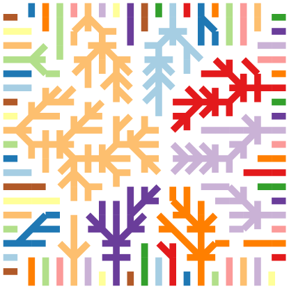
(a) Stack Order

Cells of the same colour may be run in parallel

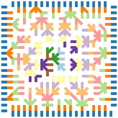
(b) Queue Order

Which Thread Processes Which Cells

Cells of the same colour are processed by the same thread

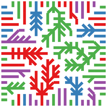
(c) Stack Order

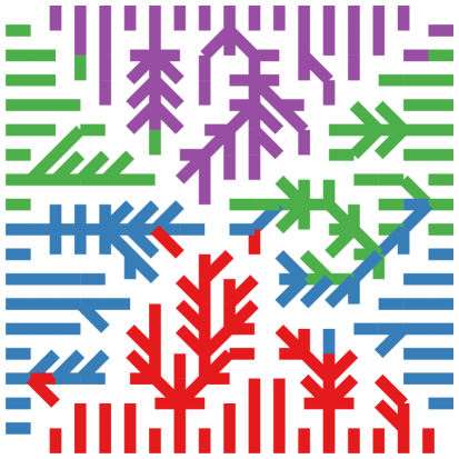
(d) Queue Order

When Cells Are Processed

Redder cells are processed later

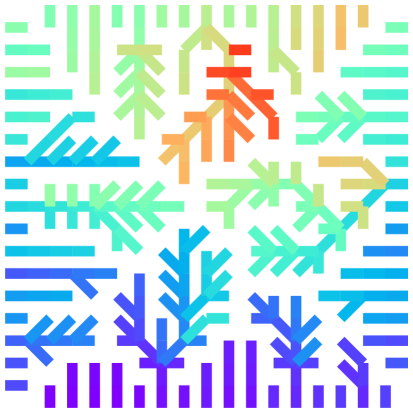
(e) Stack Order

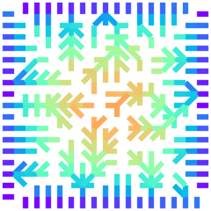
(f) Queue Order

Figure 4: Stack vs. queue: illustrated on a larger example using four threads. Note that using a stack/depth-first traversal leads to many small trees and a few large ones. This causes load imbalance and makes this form of the algorithm challenging to parallelize. In contrast, the queue can parallelize many cells at each level. The threads process 70, 71, 74, and 74 cells each in the queue example and 48, 51, 85, and 105 cells each in the stack example. Figure 3 shows a smaller example for which the algorithm is explained.

The Queue array stores the addresses of cells in the order they are to be processed. Processing the cells in this order ensures that the information needed to solve the stream power equation is always available. Each cell appears in this array once. The levels array contains indices corresponding to subdivisions of Queue. The cells in each subdivision may be processed concurrently.

Note that at this stage the algorithm differs from the B&W variant in a fundamental way: B&W uses a stack whereas I use a queue. From the perspective of graphs this is the difference between depth-first and breadth-first traversal, respectively. The difference is illustrated in Figure 3 and, again, in Figure 4. As explained in §6.1, this greatly increases potential parallelism.

To build Queue, all of the cells without receivers (the mouths of rivers and pits of depressions) are first added to the queue. A note is made in Levels of how many of these cells there are. Next, all of these cells’ donors are added and another note is made in Levels. And then the donors of the donors are added, and so on.

Parallelizing this step is difficult. It is written here as a serial algorithm. Parallelism strategies are discussed below in §9.

  Algorithm 3 Generate Queue

 

1:Let Levels be a vector that is “sufficiently long”

2:$Levels[0]\leftarrow 1$

3:$L_{s}\leftarrow 1$ $\triangleright$ Write location in Levels

4:$\textit{nqueue}\leftarrow 0$ $\triangleright$ Open location in Queue

5:

6:for all cells $c$ in $Rec$ do

7:    if $Rec[c]=\textsc{NoFlow}$ then $\triangleright$ Is it a source cell?

8:        $\textit{Queue}[\textit{nqueue}]\leftarrow c$

9:        $\textit{nqueue}\leftarrow\textit{nqueue}+1$     

10:$\textit{Levels}[L_{s}]=\textit{nqueue}$ $\triangleright$ Note last cell of Levels

11:$L_{s}\leftarrow L_{s}+1$

12:

13:$L_{L}\leftarrow-1$ $\triangleright$ Lower index of current level

14:$L_{U}\leftarrow 0$ $\triangleright$ Upper index of current level

15:while $L_{L}<L_{U}$ do

16:    $L_{L}\leftarrow L_{U}$

17:    $L_{U}\leftarrow\textit{nqueue}$

18:    for $c\in[L_{L},LU)$ do

19:        for all $k\in\textit{Dnum}[c]$ do

20:           $\textit{Queue}[\textit{nqueue}]\leftarrow\textit{donor}[\textit{Dmax}\cdot c+k]$

21:           $\textit{nqueue}\leftarrow\textit{nqueue}+1$             

22:    $\textit{Levels}[L_{s}]\leftarrow\textit{nstack}$

23:    $L_{s}\leftarrow L_{s}+1$

24:$L_{s}\leftarrow L_{s}-1$ $\triangleright$ Correct overshoot

 

5.5 Step 5: Compute Flow Accumulation

The Accum array stores the flow accumulation (also known as drainage area, contributing area, and upslope area) of each cell. As described by O’Callaghan and Mark [15] and Mark [14], the flow accumulation $A$ of a cell $c$ is defined recursively as

$$A(c)=w(c)+\sum_{n\in\mathcal{N}(c)}\alpha(n,c)A(n)$$ (2)

where $w(c)$ is the amount of flow which originates at the cell $c$; frequently, this is taken to be 1, but the value can also vary across a DEM if, for example, rainfall or soil absorption differs spatially. The summation is across all of the cell $c$’s neighbours $\mathcal{N}(c)$. $\alpha(n,c)$ represents the fraction of the neighbouring cell’s flow accumulation $A(c)$ which is apportioned to $c$. Flow may be absorbed during its downhill movement, but may only be increased by cells, so $\alpha$ is constrained such that for a given cell $c$, $\sum_{n}\alpha(c,n)\leq 1$. Flow accumulation may be parallelized across each level of the queue (see Fig. 4b).

  Algorithm 4 Flow Accumulation

 

1:Let $A$ have the same dimensions as $Elev$

2:Initialize $A$ to $\Delta x\Delta y$

3:

4:for $l\in[L_{s}-2,0]$ do

5:    for_∥ $c\in[\textit{Levels}[l],\textit{Levels}[l+1])$

6:        for $i\in[0,\textit{Dnum}[c])$ do

7:           $n\leftarrow Donor[\textit{Dmax}\cdot c+i]$

8:           $A[c]\leftarrow A[c]+A[n]$             

 

5.6 Step 6: Uplift

Tectonic uplift is incorporated in a straight-forward manner: every cell is elevated at some rate $\hat{u}$. (Note that parallelism is still trivial if uplift varies spatially.)

  Algorithm 5 Uplift

 

1:for_∥ all cells $c$ in the interior of $Elev$

2:    $Elev[c]\leftarrow Elev[c]+\hat{u}\Delta t$

 

5.7 Step 7: Calculate Erosion

Finally, erosion is calculated by implementing the Newton-Raphson method [5]. Note that the cells within each level are neither receivers nor donors of each other. More importantly, there is no causal connection between them. This means that all of the cells in a level can be executed in parallel, as in Algorithm 5.7, Line 2. Note that the tolerance check on Line 11 could be replaced with a fixed number of loops if the maximum number required were known.

  Algorithm 6 Calculate erosion

 

1:for $l\in[1,L_{s})$ do

2:    for_∥ $i\in[\textit{Levels}[l],\textit{Levels}[l+1])$

3:        $c\leftarrow\textit{Queue}[i]$ $\triangleright$ Current focal cell

4:        $n\leftarrow Rec[c]$ $\triangleright$ Neighbour of focal cell

5:        $F\leftarrow K\cdot\Delta t\cdot\textit{Acc}[c]^{m}/\textrm{dist}(n,c)^{n}$

6:        $h_{0}\leftarrow\textit{Elev}[c]$ $\triangleright$ Elevation of focal cell

7:        $h_{n}\leftarrow\textit{Elev}[n]$ $\triangleright$ Elevation of neighbour cell

8:        $h_{\textrm{new}}\leftarrow h_{0}$ $\triangleright$ Current updated value of $Elev[c]$

9:        $h_{p}\leftarrow h_{0}$ $\triangleright$ Previous updated value of $Elev[c]$

10:        $\delta\leftarrow 2\epsilon$ $\triangleright$ Difference between updated values

11:        while $|\delta|>\epsilon$ do $\triangleright$ While difference $>$ tolerance

12:           $h_{\textrm{new}}\leftarrow h_{\textrm{new}}-(h_{\textrm{new}}-h_{0}+F\cdot(h_{\textrm{new}}-h_{n})^{n})/(1+F\cdot n\cdot(h_{\textrm{new}}-h_{n})^{n-1})$

13:           $\delta\leftarrow h_{\textrm{new}}-h_{p}$ $\triangleright$ Update difference

14:           $h_{p}\leftarrow h_{\textrm{new}}$ $\triangleright$ New previous value         

15:        $Elev[c]\leftarrow h_{\textrm{new}}$ $\triangleright$ New elevation for focal cell     

 

5.8 Rinse, Repeat

All of the above steps, excluding initialization, are repeated as many times as necessary until the desired interval of time has been simulated.

6 The Improvements, Explained

6.1 Breadth-first Traversal

As described above, the this new variant of the B&W algorithm utilizes a breadth-first traversal rather than the depth-first traversal used in the original algorithm. That is: level sets are formed, rather than rooted trees. Figure 3 depicts the difference between these on a small sample drawn from Braun and Willett [5]; however, focusing on this small sample obscures important meta-level properties of the algorithms which are only visible on larger datasets such as that shown in Figure 4.

As Figure 4 shows, processing stacks in parallel, as suggested by [5], initially results in a high degree of parallelism (equal to the number of edge cells of the elevation model). However, many of the stacks are small. As a result, much of the available parallelism is quickly exhausted until a single thread is operating on a single, usually large, stack. This is known as load imbalance, and is a serious problem in parallel computing.

One way to overcome this is to launch a new parallel task every time a tree branches; eventually, all of the available parallelism will be used. However, this is not a good solution: there is a significant overhead, on the order of microseconds, to starting OpenMP tasks. [6] Since each task would process a single node, the overhead of starting a task is likely to exceed the work done by that task. Another potential solution is to only launch tasks when large trees branch. But this begs the question of how big a tree should be and how long it would take to determine which trees to branch.

In contrast, a breadth-first traversal provides an easy route to guaranteed parallelism. Since each cell donates to at most one receiver, the donors of the base level cells can all be processed in parallel, as can the donors of the donors, and so on. At each level the set of independent cells is exactly known and easily identified.

Parallelism can be realized in one of several ways. First, on a single core, SIMD (single-instruction, multiple-data) instructions can be used. These allow the same operation to be applied to several elements of an array at once. The latest such instruction set, AVX-512, can process 16 single-precision or 8 double-precision values at once. The B&W algorithm cannot take advantage of SIMD since each thread operates on a separate tree and each tree is inherently sequential.

Second, OpenMP may be used to easily divide an array between separate threads/cores. This permits the full power of a CPU to be used. For example, the new Summit supercomputer at Oak Ridge National Lab has 96 SIMD units per socket, allowing for up to 1,536 single-precision cells to be processed at once. In contrast, each socket has only 24 cores, which is the maximum parallelism that could be applied to the original B&W algorithm.

Third, GPUs provide an avenue to even greater parallelism. The Nvidia Volta GPUs used by Summit allow for approximately 5120 simultaneous floating-point operations. Each node has several GPUs.

Thus, the design of the B&W algorithm limits parallelism to tens of cells at a time, whereas the new design presented here permits many thousands of simultaneous operations.

6.2 Local Minima

It is often desirable to calculate flow directions only after internally-draining regions of a digital elevation model such as depressions and pits (see Lindsay [12] for a typology) have been eliminated. This ensures that all flows reach the edge of the model. Depressions may arise spuriously from random initial conditions, or may also represent endorheic basins. Regardless, they are usually a transient feature.

Depressions may be dealt with in one of three ways.

• They can be ignored. Over time, the model’s erosive processes will either fill them or create outlets.

• The depressions can be filled to the level of their lowest outlets. This is the method recommended by Braun and Willett [5], who suggest an $O(N\sqrt{N})$ algorithm. This is suboptimal. Optimal theoretical and empirical performance is achieved by the Priority-Flood algorithm identified in a review by Barnes et al. [4]. On integer (or appropriately discretized floating-point) data Priority-Flood runs in $O(N)$ time. For general floating-point data, it runs in $O(m\log m)$ time where $m\ll N$. Recent work by Zhou et al. [28] and Wei et al. [26] has led to significant reductions in run-time. For larger models, Barnes [1] presents an optimal parallelization of Priority-Flood.

• Depressions which are small or shallow may be breached by cutting a channel from a depression’s pit to some point beyond its outlet, as detailed by Lindsay [12].

The filling of depressions may result in flat regions where there is no locally-defined flow direction. If desired, such regions may be resolved either (a) as part of Priority-Flood [4] or (b) by routing flow both away from higher terrain and towards lower terrain [3].

6.3 Larger Models

For truly large elevation models, Barnes [1] and Barnes [2] describe optimal parallel algorithms for performing depression-filling and flow accumulation. These algorithms can efficiently process trillions of cells. Although such datasets are presently larger than those used in the context of landscape evolution, they may be of interest in the future.

7 Multiple Flow Directions

Figure 5: Multiple-flow directions. When multiple-flow directions are present a cell may have multiple receivers. All of a focal cell’s receivers must be processed before the focal cell can be processed. In the figure above it is clear that this necessitates the queue order used in the new algorithm. Cells are numbered in the order they should be processed.

The B&W uses the D8 flow router [15, 14]. This models flow as descending along the path of steepest slope from a cell to a single one of its neighbours (provided there is a local gradient). This implies the convenient property that flows only converge and never diverge. As a result, each cell has only a single receiver and Equation 1 is solved with respect to only a single pair of cells: one upslope, the other down. Multiple-flow direction (MFD) routers [19, 9, 10, 18, 21, 23, 17, 16] break this assumption. As Figure 5 shows, the queue used by the new algorithm is the right choice for working with MFD.

8 Empirical Tests

8.1 Implementations

For testing, I have developed the following implementations:

• B&W: The B&W serial algorithm described by [5] adapted from code provided by Braun.

• B&W+P: The B&W algorithm with only erosion parallelized.

• B&W+PI: The B&W algorithm parallelized using the additional techniques described here, but still using the stack structure.

• RB: A serial version of the new algorithm.

• RB+P: The new algorithm with only erosion parallelized, for comparison against B&W+P.

• RB+PI: The new algorithm using all the parallel techniques described here.

• RB+PQ: The new algorithm using all the parallel techniques described here separated by threads.

• RB+GPU: The new algorithm using all the parallel techniques described here implemented for use on a GPU.

In lieu of further details here, extensively-commented source code for all implementations is available at https://github.com/r-barnes/Barnes2018-Landscape. All algorithms were targeted to the native architecture of the test machines and compiled using GCC (except where noted) with both full optimizations and “fast math” enabled. A makefile is provided with the source code.

Minimal effort has been put into low-level optimizations and OpenACC has been used instead of more expressive, but more difficult to use, accelerator frameworks such as CUDA and OpenCL. This is intentional: the code here is meant to be accessible to any HPC-orientated geoscientist and the wall-times reflect this.

8.2 Machines

The SummitDev supercomputer of Oak Ridge National Lab’s Leadership Computing Facility was used for timing tests. Each node has two 10-core IBM POWER8 CPUs with each core supporting 8 hardware threads (160 threads total). Each node has 500GB DDR4 memory and is attached to 4 NVIDIA Tesla P100 GPUs. Cache sizes are L1=64K, L2=512K, L3=8,192K.

8.3 Test Data

Several sizes of square rasters of elevation were generated. Each cell of the rasters was initialized to a value drawn uniformly from the range $[0,1]$. Seed values were set so that all implementations at a given size used the same data, allowing for safe intercomparison.

8.4 Test Iterations

All tests were run for 120 timesteps to better extract the effect of input size on wall-times. This is sufficient to reach steady-state for small inputs, but additional iterations would be necessary to achieve convergence on larger inputs.

8.5 Correctness

The outputs of all of the implementations have been compared and are identical. This suggests that the implementations are correct (or at least all wrong in the same way). The source code includes a script which performs this comparison automatically.

9 Results & Discussion

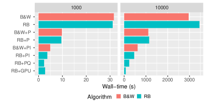
Figure 6: Timing comparisons for all implementations for two input sizes.

Figure 6 shows the aggregate of the results of the tests below. For the larger dataset, the best parallel implementations of the new algorithm run 13 x faster than the B&W serial implementation on a CPU and 43  faster on a GPU. The performance details of each implementation are discussed below. Note that $x$-axes in the figures are independent.

9.1 Serial Implementations

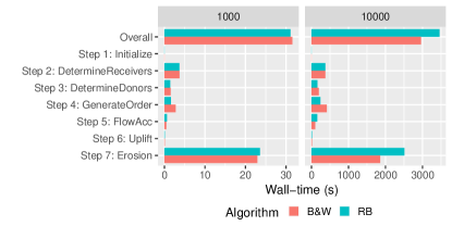
Figure 7: Timing comparisons for the B&W and RB (serial) implementations.

Figure 7 compares the wall-times of the B&W and RB implementations. These serial implementations differ only in whether or not a stack or a queue is used. Note that for the $1000^{2}$ dataset, the RB implementation is slightly faster, but that it is slower for the $10000^{2}$ dataset. This indicates that for most models using the breadth-first (queue) traversal should have a negligible impact on speed versus using the depth-first (stack) traversal. As we will see, the breadth-first traversal gives shorter wall-times when parallelism is used.

Figure 7 also shows that the majority of the wall-time (an average of 75%) is consumed by the erosion function. Optimizing this is therefore key to improving the efficiency of both algorithms.

9.2 Parallelizing Erosion

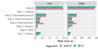
Figure 8: Timing comparisons for the B&W+P and RB+P implementations, in which only Step 7: Erosion is parallelized.

The hour-plus wall-time of the larger model in the previous section demonstrates the need for parallelism. The B&W+P and RB+P implementations address this by parallelizing the erosion function. As shown in Figure 8, doing so brings the two algorithms to approximately the same wall-time: 10 s for the $1000^{2}$ dataset and 1200 s for the $10,000^{2}$ dataset, a 66% reduction versus serial performance. For these implementations, erosion takes about 25% of the wall-time.

9.3 Parallelizing All Steps

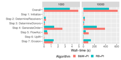
Figure 9: Timing comparisons for the B&W+PI and RB+PI implementations, in which all steps of the algorithm are parallelized.

The flat distribution of wall-times across the various steps of the RB+P and B&W+P implementations shown in the previous section indicate the need to parallelize all of the steps in order to improve efficiency. The results of doing so are shown in Figure 9. Wall-times are halved versus the previous step and the RB+PI algorithm is now definitively faster.

Profiling of RB+PI shows that synchronization at barriers (discussed earlier) is responsible for most of the time taken by both the erosion and flow accumulation steps.

The construction of the queue/stack (Step4_GenerateOrder) has now emerged as a serious bottleneck. At this point it is still serial in both algorithms. Parallelizing its construction in B&W by avoiding explicit stack construction via OpenMP tasks did not lead to better performance, though the code for this is provided. Thus, we have reached the limit of parallel gains in the B&W algorithm. However, it is possible to make further improvements to the RB algorithm.

9.4 Independent Parallelism

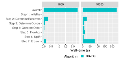
Figure 10: Timings for the RB+PQ implementation, in which separate threads have private memories.

Queue generation can be parallelized and synchronization barriers eliminated by giving each thread its own private queue in Algorithm 5.4. Passing this private queue onward to subsequent steps allows several stages of the algorithm to proceed independently. This is implemented in RB+PQ.

As Figure 10 shows, using private queues halves the run-time again. In this implementation, a barrier has been added after Step 7: Erosion which introduces a necessary synchronization delay that accounts for the majority of the wall-time not included within the steps themselves.

9.5 GPU Implementation

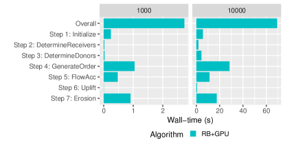
Figure 11: Timings for the RB+GPU implementation.

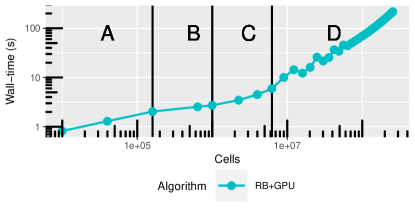
Figure 12: Scaling for the RB+GPU implementation.

	x	Edge Length	Cells
A	0.33	400	$1.6\cdot 10^{5}$
B	0.16	1000	$1.0\cdot 10^{6}$
C	0.42	2500	$6.25\cdot 10^{6}$
D	0.92	16000	$2.56\cdot 10^{8}$

Table 2: Scaling of the algorithm for the regions identified in Figure 12.

Further performance can be gained by delegating calculations to a GPU or other many-core processor. Since the GPU’s local private memory was too limited for the design of RB+PQ to work, the design of RB+PI was modified by using OpenACC directives and building with the PGI compiler.

Another possible design was to allocate global memory addressed with a thread-specific index; however, the OpenACC standard does not provide a function for obtaining such an index and the PGI compiler-specific extension __pgi_gangidx() proved difficult to work with. Similarly, though OpenMP 4.5 provides the omp_get_team_num() function, compiler support at the time of writing was too rudimentary to test this. Therefore, Step 4: Generate Order is parallelized by treating the variable nqueue in Algorithm 5.4 as an atomic with only a small number of threads used to generate the queue. Future compiler developments will, presumably, enable better design choices.

Figure 11 shows the results. For the smaller dataset, the GPU gives no wall-time advantage over the RB+PQ implementation; for the larger dataset, the GPU gives a 3 x speed-up. The scaling here is notable. A 100 x data increase in the RB+PQ implementation resulted in a 100 x increase in wall-time; in contrast, a 100 x data increase in the RB+GPU implementation resulted in only a 28 x increase in wall-time. The algorithm is scaling sublinearly.

Figure 12 and Table 2 explore this in-depth. Four distinct behavioural regions can be identified, as shown in the figure. In each region the algorithm’s wall-time scales as $O(N^{x})$ where $x$ and associated upper bounds of the edge length and number of cells of the region are shown in the table. Performance decreases smoothly throughout region $D$ eventually approaching and passing $x=1$.

The reason for this sublinearity is that the GPU has such a large amount of compute power that the smaller datasets cannot effectively use it all, so only a small fraction is applied to a given problem. The result is wall-times which remain flat as the input size increases.

The GPU has other advantages. Its unused compute power can be used to simultaneously process other models. In a multi-GPU system such as Summitdev, this means many model realizations can be carried out in a short time. GPUs also tend to be more energy-efficient than CPUs, so the net energy, environmental, and monetary costs of doing a given calculation are reduced.

9.6 Future Improvements

There are still opportunities to improve GPU performance. Step 4: Generate Order is difficult to parallelize because so little computation is done. I have handled this in my implementation by using a small number of threads to atomically increment where indices are stored in the queue. The forthcoming Nvidia Volta’s improved atomic performance may help with this situation. Otherwise, compiler improvements may allow a strategy such as RB+PQ to be implemented on GPUs in the near future.

10 Coda

The foregoing has detailed algorithmic and methodological approaches to accelerating the modeling of landscape evolution. The result is an algorithm which, in its unoptimized form, matches the performance of the previous state of the art: an algorithm by Braun and Willett [5]. On the CPU, the algorithm runs in less a third the time of the best B&W parallel implementation. On the GPU, the algorithm runs 43 x faster than the serial version of the B&W algorithm, 9 x faster the best B&W parallel implementation, and scales sublinearly with input size.

In future work, I will show how the foregoing can be extended to multi-GPU environments in order to quickly solve inverse problems and perform sensitivity analysis on landscape evolution models.

Complete source code and tests are available at https://github.com/r-barnes/Barnes2018-Landscape.

11 Acknowledgments

This work was supported by the Department of Energy’s Computational Science Graduate Fellowship (Grant No. DE-FG02-97ER25308), the National Science Foundation’s Graduate Research Fellowship, and an SC travel grant.

Empirical tests and results were performed on Summitdev, which is a prototype machine for the forthcoming Summit supercomputer managed by Oak Ridge National Laboratory’s Leadership Computing Facility, and XSEDE’s Comet supercomputer [24], which is supported by the National Science Foundation (Grant No. ACI-1053575).

Some of the techniques used in the paper were learned at the CSGF Program Review’s “Mini-GPU Hackathon” led by Fernanda Foertter, Thomas Papatheodore, Adam Simpson, Verónica Vergara Larrea, Mark Berrill, and Matthew Norman. Jack DeSlippe and Thorsten Kurth helped with an unused OpenMP implementation at an LBNL KNL Hackathon. Mat Colgrave of the PGI Compiler Group found bugs in both my code and the PGI compiler. Kelly Kochanski provided helpful discussion and ideas.

In-kind support was provided by Lorraine B., Myron B., Hannah J., Kelly K., Lydia M., Myron M., John O., and Jerry W.

12 Bibliography

References

- Barnes [2016] Barnes, R., Nov. 2016. Parallel priority-flood depression filling for trillion cell digital elevation models on desktops or clusters. Computers & Geosciences 96, 56–68. doi: 10.1016/j.cageo.2016.07.001
- Barnes [2017] Barnes, R., Jun. 2017. Parallel non-divergent flow accumulation for trillion cell digital elevation models on desktops or clusters. Environmental Modelling & Software 92, 202–212. doi: 10.1016/j.envsoft.2017.02.022
- Barnes et al. [2014a] Barnes, R., Lehman, C., Mulla, D., Jan. 2014a. An efficient assignment of drainage direction over flat surfaces in raster digital elevation models. Computers & Geosciences 62, 128–135. URL http://linkinghub.elsevier.com/retrieve/pii/S009830041300023X doi: 10.1016/j.cageo.2013.01.009
- Barnes et al. [2014b] Barnes, R., Lehman, C., Mulla, D., Jan. 2014b. Priority-flood: An optimal depression-filling and watershed-labeling algorithm for digital elevation models. Computers & Geosciences 62, 117–127. URL http://linkinghub.elsevier.com/retrieve/pii/S0098300413001337 doi: 10.1016/j.cageo.2013.04.024
- Braun and Willett [2013] Braun, J., Willett, S. D., Jan. 2013. A very efficient O(n), implicit and parallel method to solve the stream power equation governing fluvial incision and landscape evolution. Geomorphology 180-181, 170–179. URL http://linkinghub.elsevier.com/retrieve/pii/S0169555X12004618 doi: 10.1016/j.geomorph.2012.10.008
- Bull et al. [2012] Bull, J. M., Reid, F., McDonnell, N., 2012. A Microbenchmark Suite for OpenMP Tasks. In: Chapman, B. M., Massaioli, F., Müller, M. S., Rorro, M. (Eds.), OpenMP in a Heterogeneous World: 8th International Workshop on OpenMP, IWOMP 2012, Rome, Italy, June 11-13, 2012. Proceedings. Springer Berlin Heidelberg, Berlin, Heidelberg, pp. 271–274, dOI: 10.1007/978-3-642-30961-8_24. URL https://doi.org/10.1007/978-3-642-30961-8_24
- Chen et al. [2014] Chen, A., Darbon, J., Morel, J.-M., 2014. Landscape evolution models: A review of their fundamental equations. Geomorphology 219, 68 – 86. URL http://www.sciencedirect.com/science/article/pii/S0169555X14002402 doi: 10.1016/j.geomorph.2014.04.037
- Drepper [2007] Drepper, U., 2007. What every programmer should know about memory. Tech. rep., Red Hat, Inc.
- Freeman [1991] Freeman, T. G., 1991. Calculating catchment area with divergent flow based on a regular grid. Computers & Geosciences 17 (3), 413–422. URL http://www.sciencedirect.com/science/article/pii/009830049190048I
- Holmgren [1994] Holmgren, P., 1994. Multiple flow direction algorithms for runoff modelling in grid based elevation models: an empirical evaluation. Hydrological processes 8 (4), 327–334. URL http://onlinelibrary.wiley.com/doi/10.1002/hyp.3360080405/abstract
- Lague [2014] Lague, D., 2014. The stream power river incision model: evidence, theory and beyond. Earth Surface Processes and Landforms 39 (1), 38–61. URL http://dx.doi.org/10.1002/esp.3462 doi: 10.1002/esp.3462
- Lindsay [2015] Lindsay, J. B., 2015. Efficient hybrid breaching-filling sink removal methods for flow path enforcement in digital elevation models: Efficient Hybrid Sink Removal Methods for Flow Path Enforcement. Hydrological Processes 30 (6), 846–857. URL http://doi.wiley.com/10.1002/hyp.10648 doi: 10.1002/hyp.10648
- Lovecraft [1928] Lovecraft, H., Feb 1928. The Call of Cthulhu.
- Mark [1987] Mark, D. M., 1987. Chapter 4: Network models in geomorphology. In: Anderson, M. (Ed.), Modelling Geomorphological Systems. pp. 73–97.
- O’Callaghan and Mark [1984] O’Callaghan, J. F., Mark, D. M., 1984. The Extraction of Drainage Networks from Digital Elevation Data. Computer vision, graphics, and image processing 28, 323–344. URL http://dx.doi.org/10.1016/S0734-189X(84)80011-0
- Orlandini and Moretti [2009] Orlandini, S., Moretti, G., 2009. Determination of surface flow paths from gridded elevation data. Water Resources Research 45 (3). URL http://dx.doi.org/10.1029/2008WR007099 doi: 10.1029/2008WR007099
- Orlandini et al. [2003] Orlandini, S., Moretti, G., Franchini, M., Aldighieri, B., Testa, B., Jun. 2003. Path-based methods for the determination of nondispersive drainage directions in grid-based digital elevation models. Water Resources Research 39 (6). URL http://doi.wiley.com/10.1029/2002WR001639 doi: 10.1029/2002WR001639
- Pilesjö et al. [1998] Pilesjö, P., Zhou, Q., Harrie, L., Dec. 1998. Estimating Flow Distribution over Digital Elevation Models Using a Form-Based Algorithm. Annals of GIS 4 (1-2), 44–51. URL http://www.tandfonline.com/doi/abs/10.1080/10824009809480502 doi: 10.1080/10824009809480502
- Quinn et al. [1991] Quinn, P., Beven, K., Chevallier, P., Planchon, O., 1991. The Prediction Of Hillslope Flow Paths For Distributed Hydrological Modelling Using Digital Terrain Models. Hydrological Processes 5, 59–79.
- Royden and Taylor Perron [2013] Royden, L., Taylor Perron, J., 2013. Solutions of the stream power equation and application to the evolution of river longitudinal profiles. Journal of Geophysical Research: Earth Surface 118 (2), 497–518. URL http://dx.doi.org/10.1002/jgrf.20031 doi: 10.1002/jgrf.20031
- Seibert and McGlynn [2007] Seibert, J., McGlynn, B. L., Apr. 2007. A new triangular multiple flow direction algorithm for computing upslope areas from gridded digital elevation models: A NEW TRIANGULAR MULTIPLE-FLOW DIRECTION. Water Resources Research 43 (4), n/a–n/a. URL http://doi.wiley.com/10.1029/2006WR005128 doi: 10.1029/2006WR005128
- Stark et al. [2017] Stark, P., Dean, J., Norvig, P., 2017. Latency numbers every programmer should know. http://norvig.com/21-days.html#answers and https://gist.github.com/hellerbarde/2843375.
- Tarboton [1997] Tarboton, D. G., 1997. A new method for the determination of flow directions and upslope areas in grid digital elevation models. Water resources research 33 (2), 309–319.
- Towns et al. [2014] Towns, J., Cockerill, T., Dahan, M., Foster, I., Gaither, K., Grimshaw, A., Hazlewood, V., Lathrop, S., Lifka, D., Peterson, G. D., et al., 2014. Xsede: accelerating scientific discovery. Computing in Science & Engineering 16 (5), 62–74.
- Tucker and Hancock [2010] Tucker, G. E., Hancock, G. R., 2010. Modelling landscape evolution. Earth Surface Processes and Landforms 35 (1), 28–50. URL http://dx.doi.org/10.1002/esp.1952 doi: 10.1002/esp.1952
- Wei et al. [2018] Wei, H., Zhou, G., Fu, S., 2018. Efficient priority-flood depression filling in raster digital elevation models. International Journal of Digital Earth, 1–13. doi: 10.1080/17538947.2018.1429503
- Whipple and Tucker [1999] Whipple, K. X., Tucker, G. E., 1999. Dynamics of the stream-power river incision model: Implications for height limits of mountain ranges, landscape response timescales, and research needs. Journal of Geophysical Research: Solid Earth 104 (B8), 17661–17674. URL http://dx.doi.org/10.1029/1999JB900120 doi: 10.1029/1999JB900120
- Zhou et al. [2016] Zhou, G., Sun, Z., Fu, S., 2016. An efficient variant of the Priority-Flood algorithm for filling depressions in raster digital elevation models. Computers & Geosciences 90, Part A, 87 – 96. URL http://www.sciencedirect.com/science/article/pii/S0098300416300553 doi: http://dx.doi.org/10.1016/j.cageo.2016.02.021