Optimal Portfolio Design for Statistical Arbitrage in Finance

Abstract

In this paper, the optimal mean-reverting portfolio (MRP) design problem is considered, which plays an important role for the statistical arbitrage (a.k.a. pairs trading) strategy in financial markets. The target of the optimal MRP design is to construct a portfolio from the underlying assets that can exhibit a satisfactory mean reversion property and a desirable variance property. A general problem formulation is proposed by considering these two targets and an investment leverage constraint. To solve this problem, a successive convex approximation method is used. The performance of the proposed model and algorithms are verified by numerical simulations.

I Introduction

Statistical arbitrage [1] is a general quantitative investment and trading strategy widely used by many parties in the financial markets, e.g., institutional investors, hedge funds, and individual investors [2]. Since it can hedge the overall market risk, it is also referred to as a market neutral strategy [3]. In statistical arbitrage, the underlying trading basket can consist of many financial assets of different kinds such as equities, options, bonds, futures, commodities, etc. In order to arbitrage from the market, investors should buy the under-priced assets and short-sell the over-priced ones and profits will be made after the trading positions are unwound when the “mis-pricing” corrects itself. The statistical arbitrage can be traced back to the famous pairs trading [4] strategy, a.k.a. spread trading, where only two assets are considered.

In statistical arbitrage, the trading basket is used to form a “spread” characterizing the “mis-pricing” of the assets which is stationary, hence mean-reverting. To make arbitrage, trading is carried out on the mean reversion (MR) property of the spread, i.e., to buy it when it is below some statistical equilibrium and sell it when it is above the statistical equilibrium. There are many ways to design a spread, like the distance method [5], factor analysis [6], and the cointegration method [7]. In this paper, we focus on the cointegration method where the spread is discovered by time series analysis like the ordinary least squares method in [8] and the model-based methods in [9, 10]. In practice, an asset that naturally shows stationarity is also a spread [11].

The spreads from the statistical estimation methods essentially form a “cointegration subspace”. In terms of investment, a natural question is whether we can design an optimized portfolio from this subspace. Such a portfolio is named mean-reverting portfolio (MRP). To design an MRP, there are two objectives to consider: firstly the MRP should exhibit a strong MR so that it has frequent mean-crossing points and hence brings in more trading opportunities; and secondly the designed MRP should exhibit sufficient variance so that each trade can provide enough profit. These two targets naturally result in a multi-objective optimization problem, i.e., to find a desirable trade-off between MR and variance.

In [12], the author first proposed to design an MRP by optimizing an MR criterion. Later, authors in [13, 14] found that the method in [12] can result in an MRP with very low variance, then the variance control was taken into consideration. But all these works were carried out by using an $\ell_{2}$-norm constraint on the portfolio weights which do not carry a physical meaning in finance. To explicitly represent the budget allocation for different assets, the investment budget constraints were considered in [15, 16]. However, in some cases the methods in [15, 16] can lead to very large leverage (i.e., the dollar values employed) which makes it unacceptable to use for real investment. Besides that, when the variance is changed, although the investment leverage can change accordingly, the MR property of the portfolio is insensitive which makes it really hard to find a desirable trade-off between the MR and the variance properties in practice.

In this paper, a new optimal MRP design method is proposed that takes two design objectives and an explicit leverage constraint into consideration. The objective in this method can suffice to find a desirable trade-off between the MR and the variance for an MRP. Different MR criteria are considered and the portfolio constraint takes two cases into consideration. The design problem finally becomes a nonconvex constrained problem. A general algorithm based on the successive convex approximation method (SCA) is proposed. An efficient acceleration scheme is further discussed. Numerical simulations are carried out to address the efficiency of the proposed problem model and the solving algorithms.

II Mean-Reverting Portfolio (MRP) Design

For a financial asset, e.g., a stock, its price at time $t$ is denoted by $p_{t}$, and its log-price is given by $y_{t}=\log\left(p_{t}\right)$, where $\log\left(\cdot\right)$ is the natural logarithm. For $M$ assets with log-prices $\mathbf{y}_{t}=\left[y_{1,t},y_{2,t},\ldots,y_{M,t}\right]^{T}$, one (log-price) spread can be designed by the weights $\boldsymbol{\beta}=\left[\beta_{1},\beta_{2},\ldots,\beta_{M}\right]^{T}$ (say, from the cointegration model) and given by $s_{t}=\boldsymbol{\beta}^{T}\mathbf{y}_{t}$. Suppose there exists a cointegration subspace with $N$ ($N<M$) cointegration relations, i.e., $\mathbf{B}=\left[\boldsymbol{\beta}_{1};\boldsymbol{\beta}_{2};\ldots,\boldsymbol{\beta}_{N}\right]$, then we can have

$$\mathbf{s}_{t}=\mathbf{B}^{T}\mathbf{y}_{t},$$ (1)

where $\mathbf{s}_{t}$ denote $N$ spreads. Specifically, if the log-prices are stationary in nature, we get $\mathbf{s}_{t}=\mathbf{y}_{t}$ with $\mathbf{B}=\mathbf{I}$ $\left(N=M\right)$.

The objective of mean-reverting portfolio (MRP) design is to construct a portfolio of the underlying spreads to attain desirable trading properties. An MRP is defined by its portfolio weights $\mathbf{w}=\left[w_{1},w_{2},\ldots,w_{N}\right]^{T}$, with its resulting spread given by $z_{t}=\mathbf{w}^{T}\mathbf{s}_{t}=\sum_{n=1}^{N}w_{n}s_{n,t}$. Due to (1), we can get

$$\begin{array}[]{c}z_{t}=\mathbf{w}_{p}^{T}\mathbf{y}_{t}=\sum_{m=1}^{M}w_{p,m}y_{m,t},\end{array}$$ (2)

where $\mathbf{w}_{p}=\mathbf{B}\mathbf{w}$ are the MRP weights indicating the market value on different assets. For $m=1,2,\ldots,M$, $w_{p,m}>0$, $w_{p,m}<0$, and $w_{p,m}=0$ mean a long position (i.e., it is bought), a short position (i.e., it is short-sold or, more plainly, borrowed and sold), and no position on the asset, respectively.

Considering the two design objectives, i.e., MR and variance, we formulate the optimal MRP design problem as

$$\begin{array}[]{cl}\underset{\mathbf{w}}{\text{minimize}}&F\left(\mathbf{w}\right)\triangleq U\left(\mathbf{w}\right)+\mu V\left(\mathbf{w}\right)\\ \text{subject to}&\mathcal{W}=\left\{\mathbf{w}\mid\|\mathbf{B}\mathbf{w}\|_{1}\leq B\right\}.\end{array}$$ (3)

The MR criterion term $U\left(\mathbf{w}\right)$ is jointly represented as

$$\begin{array}[]{l}\>\>\>U\left(\mathbf{w}\right)\\ =\xi\frac{\mathbf{w}^{T}\mathbf{H}\mathbf{w}}{\mathbf{w}^{T}\mathbf{M}_{0}\mathbf{w}}+\zeta\left(\frac{\mathbf{w}^{T}\mathbf{M}_{1}\mathbf{w}}{\mathbf{w}^{T}\mathbf{M}_{0}\mathbf{w}}\right)^{2}+\eta\sum_{i=2}^{p}\left(\frac{\mathbf{w}^{T}\mathbf{M}_{i}\mathbf{w}}{\mathbf{w}^{T}\mathbf{M}_{0}\mathbf{w}}\right)^{2},\end{array}$$

which particularizes to the predictability statistics $\mathrm{pre}\left(\mathbf{w}\right)$ with $\xi=1$, $\mathbf{H}=\mathbf{M}_{1}^{T}\mathbf{M}_{0}^{-1}\mathbf{M}_{1}$, and $\zeta=\eta=0$; the portmanteau statistics $\mathrm{por}\left(p,\mathbf{w}\right)$ with $\xi=0$, and $\zeta=\eta=1$; the crossing statistics $\mathrm{pre}\left(\mathbf{w}\right)$ with $\xi=1$, $\mathbf{H}=\mathbf{M}_{1}$, and $\zeta=\eta=0$; and the penalized crossing statistics $\mathrm{pcro}\left(p,\mathbf{w}\right)$ with $\xi=1$, $\mathbf{H}=\mathbf{M}_{1}$, $\zeta=0$, and $\eta>0$, where $\mathbf{M}_{i}=\mathsf{Cov}\left(\mathbf{s}_{t},\mathbf{s}_{t+i}\right)$ for $i=1,\ldots,p$ [13, 16]. The variance term $V\left(\mathbf{w}\right)$ is represented by

$$\begin{array}[]{c}V\left(\mathbf{w}\right)=\frac{1}{\mathbf{w}^{T}\mathbf{M}_{0}\mathbf{w}}.\end{array}$$

And $\mu\geq 0$ defines the trade-off between the MR and variance. Specially, when $\mu=0$, the designed MRP has the best MR property; and likewise when $\mu\rightarrow\infty$, the problem leads to the MRP with best variance. In the constraint set $\mathcal{W}$, $B$ means the total leverage deployed on all the assets in an investment. The problem in (3) is a nonconvex constrained problem with a nonconvex smooth objective and a convex nonsmooth constraint.

III Problem Solving via The SCA Method

III-A The Successive Convex Approximation Method

The successive convex approximation (SCA) method [17] is a general optimization method especially for nonconvex problems. In this paper, a variant of SCA in [18] is used, which solves the original problem by solving a sequence of strongly convex problems and can also preserve feasibility of the iterates. Specifically, a problem is given as follows:

$$\begin{array}[]{cccc}\underset{\mathbf{x}}{\mathsf{minimize}}&f\left(\mathbf{x}\right)&\mathsf{subject\>to}&\mathbf{x}\in{\cal X},\end{array}$$ (4)

where ${\cal X}\subseteq\mathbb{R}^{N}$ and no assumption is on the convexity and smoothness of $f\left(\mathbf{x}\right)$ and ${\cal X}$. Instead of tackling (4) directly, starting from an initial point $\mathbf{x}^{\left(0\right)}$, the SCA method solves a series of subproblems with surrogate functions $\tilde{f}\left(\mathbf{x};\mathbf{x}^{\left(k\right)}\right)$ approximating the original objective $f\left(\mathbf{x}\right)$ and a sequence $\left\{\mathbf{x}^{\left(k\right)}\right\}$ is generated by the following rules:

$$\begin{cases}\begin{array}[]{l}\hat{\mathbf{x}}^{\left(k+1\right)}=\arg\underset{\mathbf{x}\in\mathcal{X}}{\min}\tilde{f}\left(\mathbf{x};\mathbf{x}^{\left(k\right)}\right)\\ \mathbf{x}^{\left(k+1\right)}=\mathbf{x}^{\left(k\right)}+\gamma^{\left(k\right)}\left(\hat{\mathbf{x}}^{\left(k+1\right)}-\mathbf{x}^{\left(k\right)}\right).\end{array}\end{cases}$$ (5)

The first step is to generate the descent direction (i.e., $\hat{\mathbf{x}}^{\left(k+1\right)}-\mathbf{x}^{\left(k\right)}$) by solving a best-response problem, and the second step is the variable update with step-size $\gamma^{\left(k\right)}$. For $\tilde{f}\left(\mathbf{x};\mathbf{x}^{\left(k\right)}\right)$, the following conditions are needed:

A1) given $\mathbf{x}^{\left(k\right)}$, $\tilde{f}\left(\mathbf{x};\mathbf{x}^{\left(k\right)}\right)$ is $c$-strongly convex on $\mathcal{X}$ for some $c>0$, i.e., $\nabla_{\mathbf{x}}^{2}\tilde{f}\left(\mathbf{x};\mathbf{x}^{\left(k\right)}\right)\succeq c\mathbf{I}$;

A2) $\nabla_{\mathbf{x}}\tilde{f}\left(\mathbf{x}^{\left(k\right)};\mathbf{x}^{\left(k\right)}\right)=\nabla_{\mathbf{x}}f\left(\mathbf{x}^{\left(k\right)}\right)$ for all $\mathbf{x}^{\left(k\right)}\in\mathcal{X}$

A3) $\nabla_{\mathbf{x}}\tilde{f}\left(\mathbf{x};\mathbf{x}\right)$ is continuous for all $\mathbf{x}\in\mathcal{X}$.

It is easy to see that the key point in SCA is to find a good approximation $\tilde{f}\left(\mathbf{x};\mathbf{x}^{\left(k\right)}\right)$ and to choose a proper step-size $\gamma^{\left(k\right)}$ for a fast convergence.

III-B Optimal MRP Design Based on The SCA Method

Applying the SCA method to solve problem (3), we can first have the convex approximation function $\tilde{F}(\mathbf{w};\mathbf{w}^{\left(k\right)})$ given by

$$\begin{array}[]{l}\;\;\tilde{F}\left(\mathbf{w};\mathbf{w}^{\left(k\right)}\right)\\ =\tilde{U}\left(\mathbf{w};\mathbf{w}^{\left(k\right)}\right)+\mu\tilde{V}\left(\mathbf{w};\mathbf{w}^{\left(k\right)}\right)+\tau\|\mathbf{w}-\mathbf{w}^{\left(k\right)}\|_{2}^{2},\end{array}$$ (6)

with the parameter $\tau\geq 0$ on the proximal term is added for convergence reason. To get the convex approximation $\tilde{U}\left(\mathbf{w};\mathbf{w}^{\left(k\right)}\right)$, the second and the third nonconvex terms in $U\left(\mathbf{w}\right)$ are convexified by linearizing each term inside the squares $\left(\cdot\right)^{2}$. This approximation technique ensures the same gradient for $\tilde{U}\left(\mathbf{w};\mathbf{w}^{\left(k\right)}\right)$ with $U\left(\mathbf{w}\right)$ and naturally keep the convex structure $U\left(\mathbf{w}\right)$. Then $\tilde{U}\left(\mathbf{w};\mathbf{w}^{\left(k\right)}\right)$ is given by

$$\begin{array}[]{c}\tilde{U}\left(\mathbf{w};\mathbf{w}^{\left(k\right)}\right)=\mathbf{w}^{T}\mathbf{A}_{\mathrm{U}}^{\left(k\right)}\mathbf{w}+\mathbf{b}_{\mathrm{U}}^{\left(k\right)T}\mathbf{w},\end{array}$$ (7)

where $\mathbf{A}_{\mathrm{U}}^{\left(k\right)}\triangleq 4\zeta(\mathbf{d}_{0,1}^{\left(k\right)}\mathbf{d}_{0,1}^{\left(k\right)T}+\mathbf{d}_{1,0}^{\left(k\right)}\mathbf{d}_{1,0}^{\left(k\right)T}-\mathbf{d}_{0,1}^{\left(k\right)}\mathbf{d}_{1,0}^{\left(k\right)T}-\mathbf{d}_{1,0}^{\left(k\right)}\mathbf{d}_{0,1}^{\left(k\right)T})+4\eta\sum_{i=2}^{p}(\mathbf{d}_{0,i}^{\left(k\right)}\mathbf{d}_{0,i}^{\left(k\right)T}+\mathbf{d}_{i,0}^{\left(k\right)}\mathbf{d}_{i,0}^{\left(k\right)T}-\mathbf{d}_{0,i}^{\left(k\right)}\mathbf{d}_{i,0}^{\left(k\right)T}-\mathbf{d}_{i,0}^{\left(k\right)}\mathbf{d}_{0,i}^{\left(k\right)T})$, and $\mathbf{b}_{\mathrm{U}}^{\left(k\right)}\triangleq 2\xi(\mathbf{d}_{0,h}^{\left(k\right)}-\mathbf{d}_{h,0}^{\left(k\right)})+2\zeta r_{1}^{\left(k\right)}(\mathbf{d}_{0,1}^{\left(k\right)}-\mathbf{d}_{1,0}^{\left(k\right)})+2\eta\sum_{i=2}^{p}r_{i}^{\left(k\right)}(\mathbf{d}_{0,i}^{\left(k\right)}-\mathbf{d}_{i,0}^{\left(k\right)})$, with $r_{h}^{\left(k\right)}=(\mathbf{w}^{\left(k\right)T}\mathbf{H}\mathbf{w}^{\left(k\right)})$ $/(\mathbf{w}^{\left(k\right)T}\mathbf{M}_{0}\mathbf{w}^{\left(k\right)})$, $r_{i}^{\left(k\right)}=(\mathbf{w}^{\left(k\right)T}\mathbf{M}_{i}\mathbf{w}^{\left(k\right)})/(\mathbf{w}^{\left(k\right)T}\mathbf{M}_{0}\mathbf{w}^{\left(k\right)})$, $\mathbf{d}_{0,h}^{\left(k\right)}=\mathbf{H}\mathbf{w}^{\left(k\right)}/(\mathbf{w}^{\left(k\right)T}\mathbf{M}_{0}\mathbf{w}^{\left(k\right)})$, $\mathbf{d}_{h,0}^{\left(k\right)}=r_{h}^{\left(k\right)}\mathbf{M}_{0}\mathbf{w}^{\left(k\right)}$, $\mathbf{d}_{0,i}^{\left(k\right)}=\mathbf{M}_{i}\mathbf{w}^{\left(k\right)}$ $/(\mathbf{w}^{\left(k\right)T}\mathbf{M}_{0}\mathbf{w}^{\left(k\right)})$, and $\mathbf{d}_{i,0}^{\left(k\right)}=r_{i}^{\left(k\right)}\mathbf{M}_{0}\mathbf{w}^{\left(k\right)}$, with $i=1,\ldots,p$. Likewise, the $\tilde{V}\left(\mathbf{w};\mathbf{w}^{\left(k\right)}\right)$ is the convex approximation for the variance term $V\left(\mathbf{w}\right)$ which is given by

$$\begin{array}[]{c}\tilde{V}\left(\mathbf{w};\mathbf{w}^{\left(k\right)}\right)=\mathbf{b}_{\mathrm{V}}^{\left(k\right)T}\mathbf{w},\end{array}$$ (8)

where $\mathbf{b}_{\mathrm{V}}^{\left(k\right)}\triangleq-2\left(\mathbf{w}^{\left(k\right)T}\mathbf{M}_{0}\mathbf{w}^{\left(k\right)}\right)^{-2}\mathbf{M}_{0}\mathbf{w}^{\left(k\right)}$.

Then by combining $\tilde{U}\left(\mathbf{w};\mathbf{w}^{\left(k\right)}\right)$ with $\tilde{V}\left(\mathbf{w};\mathbf{w}^{\left(k\right)}\right)$ and dropping some constants, the $\tilde{F}\left(\mathbf{w};\mathbf{w}^{\left(k\right)}\right)$ in (6) becomes

$$\tilde{F}\left(\mathbf{w};\mathbf{w}^{\left(k\right)}\right)=\mathbf{w}^{T}\mathbf{A}^{\left(k\right)}\mathbf{w}+\mathbf{b}^{\left(k\right)T}\mathbf{w},$$ (9)

where $\mathbf{A}^{\left(k\right)}\triangleq\mathbf{A}_{\mathrm{U}}^{\left(k\right)}+\tau\mathbf{I}$, and $\mathbf{b}^{\left(k\right)}\triangleq\mathbf{b}_{\mathrm{U}}^{\left(k\right)}+\mu\mathbf{b}_{\mathrm{V}}^{\left(k\right)}-2\tau\mathbf{w}^{\left(k\right)}$. And the subproblem to solve becomes

$$\begin{array}[]{cl}\underset{\mathbf{w}}{\text{minimize}}&\mathbf{w}^{T}\mathbf{A}^{\left(k\right)}\mathbf{w}+\mathbf{b}^{\left(k\right)T}\mathbf{w}\\ \text{subject to}&\|\mathbf{B}\mathbf{w}\|_{1}\leq B,\end{array}$$ (10)

which is a convex problem. Summarizing, in order to solve the original problem (3), we just need to iteratively solve a sequence of convex problems (10). The SCA-based algorithm is named SCA-MRP and given in Algorithm 1. The convergence of Algorithm 1 can be guaranteed if the step-size $\gamma^{\left(k\right)}$ is chosen as a (suitably small) constant or alternatively chosen according to the following diminishing step-size rule:

$$\begin{array}[]{cl}\text{Given}&\gamma^{\left(0\right)}\in\left(0,1\right],\\ \text{Let}&\gamma^{\left(k+1\right)}=\gamma^{\left(k\right)}\left(1-\theta\gamma^{\left(k\right)}\right)\;\text{for }k=0,1,2,\ldots,\end{array}$$

where $\theta\in\left(0,1\right)$ is a given constant.

1:$\mathbf{H}$, $\mathbf{M}_{i}$ $(i=0,\ldots,p)$, $\mu$, $\mathbf{B}$, $B$ and $\tau$

2:Set $k=0$, $\gamma^{(0)}$ and $\mathbf{w}^{(0)}$.

3:repeat

4:     Compute $\mathbf{A}^{(k)}$ and $\mathbf{b}^{(k)}$.

5:     $\hat{\mathbf{w}}^{(k+1)}=\arg\underset{\mathbf{w}\in\mathcal{W}}{\min}\mathbf{w}^{T}\mathbf{A}^{(k)}\mathbf{w}+\mathbf{b}^{(k)T}\mathbf{w}$

6:     $\mathbf{w}^{(k+1)}=\mathbf{w}^{(k)}+\gamma^{(k)}(\hat{\mathbf{w}}^{(k+1)}-\mathbf{w}^{(k)})$

7:     $k\leftarrow k+1$

8:until convergence

Algorithm 1 SCA-MRP Algorithm for Optimal MRP Design

The inner convex problem (see $\mathtt{Step}$ $\mathtt{5}$ in Algorithm 1) has no closed-form solution, but we can resort to the off-the-shelf solvers like $\mathtt{MOSEK}$ [19] or the popular scripting language $\mathtt{CVX}$ [20]. However, as an alternative to the general-purpose methods, we can also develop problem-specific algorithms to solve this problem efficiently.

III-C Solving The Inner Subproblem in SCA Using ADMM

The alternating direction method of multipliers (ADMM) is widely used to solve convex problems by breaking them into smaller parts, each of which is then easier to handle [21]. To solve problem (10) by ADMM, we first rewrite problem (10) (for notational simplicity, superscripts $\left(k\right)$ are omitted) by introducing an auxiliary variable $\mathbf{z}=\mathbf{B}\mathbf{w}$ as follows:

$$\begin{array}[]{cl}\underset{\mathbf{w},\mathbf{z}}{\text{minimize}}&\mathbf{w}^{T}\mathbf{A}\mathbf{w}+\mathbf{b}^{T}\mathbf{w}\\ \text{subject to}&\|\mathbf{z}\|_{1}\leq B,\;\mathbf{B}\mathbf{w}-\mathbf{z}=\mathbf{0}.\end{array}$$ (11)

Then the augmented Lagrangian is

$$\begin{array}[]{l}\;\;L_{\rho}\left(\mathbf{w},\mathbf{z},\mathbf{u}\left(\mathbf{y}\right)\right)\\ =\mathbf{w}^{T}\mathbf{A}\mathbf{w}+\mathbf{b}^{T}\mathbf{w}+I_{\mathcal{C}}(\mathbf{z})+\frac{\rho}{2}\left\|\mathbf{P}\mathbf{w}-\mathbf{z}+\mathbf{u}\right\|_{2}^{2},\end{array}$$

where $I_{\mathcal{C}}\left(\mathbf{z}\right)=\left\{\begin{array}[]{l}0,\quad\mathbf{z}\in\mathcal{C}\\ +\infty,\text{otherwise}\end{array}\right.$ with $\mathcal{C}\triangleq\left\{\mathbf{z}\big{|}\left\|\mathbf{z}\right\|_{1}\leq B\right\}$ is the indicator function and the penalty parameter $\rho>0$ serves as the dual update step-size with the scaled dual variable $\mathbf{u}=\frac{1}{\rho}\mathbf{y}$. Then, the ADMM updates are given in three variable blocks, i.e., ($\mathbf{w},\mathbf{z},\mathbf{u}\left(\mathbf{y}\right)$), by

$$\begin{cases}\begin{array}[]{l}\mathbf{w}^{\left(k+1\right)}=\arg\underset{\mathbf{w}}{\min}\Bigl{\{}\mathbf{w}^{T}\mathbf{A}\mathbf{w}+\mathbf{b}^{T}\mathbf{w}\\ \quad\quad\quad\quad\quad\quad\quad\quad\quad\quad\quad\quad+\frac{\rho}{2}\left\|\mathbf{B}\mathbf{w}-\mathbf{z}^{\left(k\right)}+\mathbf{u}^{\left(k\right)}\right\|_{2}^{2}\Bigr{\}}\\ \mathbf{z}^{\left(k+1\right)}=\arg\underset{\mathbf{z}}{\min}\left\{I_{\mathcal{C}}(\mathbf{z})+\frac{\rho}{2}\left\|\mathbf{z}-\mathbf{B}\mathbf{w}^{\left(k+1\right)}-\mathbf{u}^{\left(k\right)}\right\|_{2}^{2}\right\}\\ \mathbf{u}^{\left(k+1\right)}=\mathbf{u}^{\left(k\right)}+\mathbf{B}\mathbf{w}^{\left(k+1\right)}-\mathbf{z}^{\left(k+1\right)}.\end{array}\end{cases}$$

Specifically, for variable $\mathbf{w}$, it is to solve a convex quadratic programming with a closed-form solution as follows:

$$\mathbf{w}^{\left(k+1\right)}=-\left(2\mathbf{A}+\rho\mathbf{B}^{T}\mathbf{B}\right)^{-1}\left(\mathbf{b}+\rho\mathbf{B}^{T}\left(\mathbf{u}^{\left(k\right)}-\mathbf{z}^{\left(k\right)}\right)\right).$$

By defining $\mathbf{h}^{\left(k\right)}=\mathbf{B}\mathbf{w}^{\left(k+1\right)}+\mathbf{u}^{\left(k\right)}$, the variable $\mathbf{z}$ update is equivalent to solve

$$\begin{array}[]{c}\mathbf{z}^{\left(k+1\right)}=\arg\underset{\mathbf{z}\in\mathcal{C}}{\min}\left\|\mathbf{z}-\mathbf{h}^{\left(k\right)}\right\|_{2}^{2}=\Pi_{\mathcal{C}}\left(\mathbf{h}^{\left(k\right)}\right),\end{array}$$ (12)

which is the classical projection onto the $\ell_{1}$-ball problem [22, 23] with $\Pi_{\mathcal{C}}\left(\cdot\right)$ denoting the projection operator. This problem has a closed-form solution given in the following.

if $||\mathbf{h}||_{1}\leq B$ then

     $\mathbf{z}=\mathbf{h}$, return $\mathbf{z}$

else

     $\mathbf{a}=\mathrm{sign}(\mathbf{h})$ and $\mathbf{b}=\mathrm{abs}(\mathbf{h})$

     Sort $\mathbf{b}$ in order: $b_{(1)}\geq b_{(2)}\geq\dots\geq b_{(N)}$

     $\rho=\arg\underset{1\leq j\leq N}{\max}\bigg{\{}b_{(j)}-\frac{1}{j}\Big{(}\sum_{i=1}^{j}b_{(i)}-B\Big{)}>0\bigg{\}}$

     $\theta=\frac{1}{\rho}\Big{(}\sum_{i=1}^{\rho}b_{(i)}-B\Big{)}$

     $z_{j}=a_{j}\max\{b_{j}-\theta,0\}$, $1\leq j\leq N$, return $\mathbf{z}$

end if

Algorithm 2 Projection onto the $\ell_{1}$-ball.

In the solution for $\mathbf{z}$-update, $\mathrm{sgn}\left(\cdot\right)$ is the “sign function”; $\mathrm{abs}\left(\cdot\right)$ is the absolute value function; and $b_{(j)}$ $\left(1\leq j\leq N\right)$ denotes the $j$-th largest element in $\mathbf{b}$. Then, the overall ADMM-based algorithm can be summarized in Algorithm 3.

1:$\mathbf{A}$, $\mathbf{b}$, $\mathbf{B}$, $B$ and $\rho$

2:Set $\mathbf{w}^{(0)}$, $\mathbf{z}^{(0)}$, $\mathbf{u}^{(0)}$ and $k=0$.

3:repeat

4:     $\mathbf{w}^{(k+1)}=-(2\mathbf{A}+\rho\mathbf{B}^{T}\mathbf{B})^{-1}(\mathbf{b}+\rho\mathbf{B}^{T}(\mathbf{u}^{(k)}-\mathbf{z}^{(k)}))$

5:     $\mathbf{h}^{(k)}=\mathbf{B}\mathbf{w}^{(k+1)}+\mathbf{u}^{(k)}$

6:     $\mathbf{z}^{(k+1)}=\Pi_{\mathcal{C}}(\mathbf{h}^{(k)})$

7:     $\mathbf{u}^{(k+1)}=\mathbf{u}^{(k)}+\mathbf{B}\mathbf{w}^{(k+1)}-\mathbf{z}^{(k+1)}$

8:     $k\leftarrow k+1$

9:until convergence

Algorithm 3 An ADMM-Based Algorithm for Problem (10)

III-D Acceleration Scheme for The SCA-MRP Algorithm

Besides the diminishing step-size rules for step-size $\gamma^{\left(k\right)}$, it is possible to get a better convergence speed for Algorithm 1 by using some acceleration method. One Armijo-like backtracking line search rule for the step-size [24] is given as follows:

$$\begin{array}[]{cl}\mathrm{Given}&\alpha,\beta\in\left(0,1\right),\;l=0\\ \mathrm{While}&\Delta F\left(\mathbf{w}^{\left(k\right)}\right)>-\alpha\beta^{l}\|\Delta\mathbf{w}^{\left(k\right)}\|_{2}^{2}\\ &\quad l=l+1\\ \mathrm{Let}&\gamma^{\left(k\right)}=\beta^{l}\;\text{for }k=0,1,2,\ldots,\end{array}$$

where $\Delta F\left(\mathbf{w}^{\left(k\right)}\right)=F\left(\mathbf{w}^{\left(k\right)}+\beta^{l}\Delta\mathbf{w}^{\left(k\right)}\right)-F\left(\mathbf{w}^{\left(k\right)}\right)$ with $\Delta\mathbf{w}^{\left(k\right)}=\hat{\mathbf{w}}^{\left(k+1\right)}-\mathbf{w}^{\left(k\right)}$.

IV Numerical Simulations

In this section, we test the proposed problem formulation and algorithms using market data from the Standard & Poor’s 500 (S&P 500) Index, which are retrieved from Google Finance. We choose stock candidates into one asset pool as {$\mathsf{APA}$, $\mathsf{AXP}$, $\mathsf{CAT}$, $\mathsf{COF}$, $\mathsf{FCX}$, $\mathsf{IBM}$, $\mathsf{MMM}$}, where they are denoted by their ticker symbols in Figure 1. Three spreads are constructed from this pool based on the Johansen method as shown in Figure 1. The methods proposed in this paper are employed for optimal MRP design. After that, we apply the designed MRP to a mean reversion trading based on the trading framework and performance measure introduced in [16]. In Figure 1, we compare the performance of our designed MRP with spread $s_{2}$. The performance metrics like return on investment (ROI), Sharpe ratio, and cumulative P&Ls are reported. It is shown that the designed MRP can achieve a higher Sharpe ratio and a better final cumulative return.

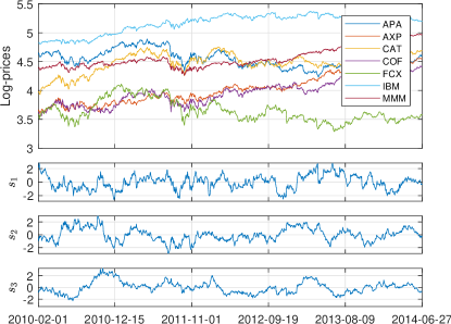
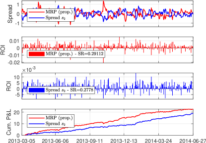
Figure 1: A mean-reversion trading based on real data.

We further show the convergence property over iterations of the objective function value in problem (3) by using the proposed SCA-MRP algorithm with and without acceleration in comparison to some benchmark algorithms.

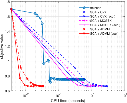
Figure 2: Convergence comparison for objective function value.

The SCA-MRP algorithm is first compared with the general purpose constrained optimization solver $\mathtt{fmincon}$ [25] in MATLAB. From Figure 2, it is easy to see that SCA-MRP obtains a faster convergence and converges to a better solution than $\mathtt{fmincon}$. We further compare the SCA-MRP with the inner problem solved by $\mathtt{CVX}$, $\mathtt{MOSEK}$, and ADMM. The inner problem solved by ADMM can uniformly get a faster convergence either using acceleration or not than the others. In Figure 3, we show that by tuning the parameter $\mu$ in problem (3), our formulation is able to get a trade-off between MR and variance of the portfolio. However, this desirable property cannot be attained with existing methods in the literature.

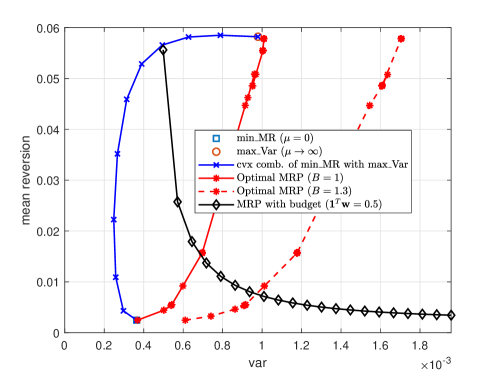
Figure 3: Trade-off between MR and variance in MRP design.

V Conclusions

The optimal mean-reverting portfolio design problem arising from statistical arbitrage has been considered in this paper. We first proposed a general model for MRP design where a trade-off can be attained between the MR and variance of an MRP and the investment leverage constraint is considered. To solve the problem, a SCA-based algorithm is used with the inner convex subproblem efficiently solved by ADMM. Numerical results show that our proposed method can generate consistent profits and outperform the benchmark methods.

References

• [1] A. Pole, Statistical Arbitrage: Algorithmic trading insights and techniques.   John Wiley & Sons, 2011, vol. 411.
• [2] C. Krauss, “Statistical arbitrage pairs trading strategies: Review and outlook,” Journal of Economic Surveys, vol. 31, no. 2, pp. 513–545, 2017.
• [3] B. I. Jacobs and K. N. Levy, Market Neutral Strategies.   John Wiley & Sons, 2005, vol. 112.
• [4] G. Vidyamurthy, Pairs Trading: Quantitative methods and analysis.   John Wiley & Sons, 2004, vol. 217.
• [5] E. Gatev, W. N. Goetzmann, and K. G. Rouwenhorst, “Pairs trading: Performance of a relative-value arbitrage rule,” Review of Financial Studies, vol. 19, no. 3, pp. 797–827, 2006.
• [6] M. Avellaneda and J.-H. Lee, “Statistical arbitrage in the US equities market,” Quantitative Finance, vol. 10, no. 7, pp. 761–782, 2010.
• [7] J. Caldeira and G. V. Moura, “Selection of a portfolio of pairs based on cointegration: A statistical arbitrage strategy,” Available at SSRN 2196391, 2013.
• [8] R. F. Engle and C. W. Granger, “Co-integration and error correction: Representation, estimation, and testing,” Econometrica: Journal of the Econometric Society, pp. 251–276, 1987.
• [9] S. Johansen, “Estimation and hypothesis testing of cointegration vectors in gaussian vector autoregressive models,” Econometrica: Journal of the Econometric Society, pp. 1551–1580, 1991.
• [10] Z. Zhao and D. P. Palomar, “Robust maximum likelihood estimation of sparse vector error correction model,” in Proc. the 2017 5th IEEE Global Conference on Signal and Information Processing, Montreal, QB, Canada, Nov. 2017, pp. 913–917.
• [11] H. Zhang and Q. Zhang, “Trading a mean-reverting asset: Buy low and sell high,” Automatica, vol. 44, no. 6, pp. 1511–1518, 2008.
• [12] A. d’Aspremont, “Identifying small mean-reverting portfolios,” Quantitative Finance, vol. 11, no. 3, pp. 351–364, 2011.
• [13] M. Cuturi and A. d’Aspremont, “Mean reversion with a variance threshold,” in Proc. of the 30th Int. Conf. on Machine Learning (ICML-13), Atlanta, USA, Jun. 2013, pp. 271–279.
• [14] ——, “Mean-reverting portfolios,” in Financial Signal Processing and Machine Learning, A. N. Akansu, S. R. Kulkarni, and D. M. Malioutov, Eds.   John Wiley & Sons, 2016, ch. 3, pp. 23–40.
• [15] Z. Zhao and D. P. Palomar, “Mean-reverting portfolio design via majorization-minimization method,” in 2016 50th Asilomar Conf. Signals Proc. Systems and Computers, Pacific Grove, CA, USA, Nov. 2016, pp. 1530–1534.
• [16] ——, “Mean-reverting portfolio with budget constraint,” IEEE Transactions on Signal Processing, vol. PP, no. 99, p. 1, 2018.
• [17] B. R. Marks and G. P. Wright, “A general inner approximation algorithm for nonconvex mathematical programs,” Operations Research, vol. 26, no. 4, pp. 681–683, 1978.
• [18] G. Scutari, F. Facchinei, P. Song, D. P. Palomar, and J.-S. Pang, “Decomposition by partial linearization: Parallel optimization of multi-agent systems,” IEEE Transactions on Signal Processing, vol. 62, no. 3, pp. 641–656, 2014.
• [19] A. MOSEK, The MOSEK optimization toolbox for MATLAB manual Version 7.1 (Revision 28), 2015.
• [20] M. Grant, S. Boyd, and Y. Ye, “CVX: Matlab software for disciplined convex programming,” 2008.
• [21] S. Boyd, N. Parikh, E. Chu, B. Peleato, and J. Eckstein, “Distributed optimization and statistical learning via the alternating direction method of multipliers,” Foundations and Trends® in Machine Learning, vol. 3, no. 1, pp. 1–122, 2011.
• [22] D. P. Palomar, “Convex primal decomposition for multicarrier linear mimo transceivers,” IEEE Transactions on Signal Processing, vol. 53, no. 12, pp. 4661–4674, 2005.
• [23] J. Duchi, S. Shalev-Shwartz, Y. Singer, and T. Chandra, “Efficient projections onto the $\ell_{1}$-ball for learning in high dimensions,” in Proceedings of the 25th International Conference on Machine Learning.   ACM, 2008, pp. 272–279.
• [24] G. Scutari, F. Facchinei, and L. Lampariello, “Parallel and distributed methods for constrained nonconvex optimization-Part I: Theory.” IEEE Transactions on Signal Processing, vol. 65, no. 8, pp. 1929–1944, 2017.
• [25] T. Coleman, M. A. Branch, and A. Grace, “Optimization toolbox,” For Use with MATLAB. User’s Guide for MATLAB 5, Version 2, Relaese II, 1999.