Rigorous numerical computations for 1D advection equations with variable coefficients

Abstract

This paper provides a methodology of verified computing for solutions to 1-dimensional advection equations with variable coefficients. The advection equation is typical partial differential equations (PDEs) of hyperbolic type. There are few results of verified numerical computations to initial-boundary value problems of hyperbolic PDEs. Our methodology is based on the spectral method and semigroup theory. The provided method in this paper is regarded as an efficient application of semigroup theory in a sequence space associated with the Fourier series of unknown functions. This is a foundational approach of verified numerical computations for hyperbolic PDEs. Numerical examples show that the rigorous error estimate showing the well-posedness of the exact solution is given with high accuracy and high speed.

Keywords: 1D variable coefficient advection equation, verified numerical computation, $C_{0}$ semigroup, rigorous error bound, Fourier-Chebyshev spectral method

AMS subject classifications : 65G40, 65M15, 65M70, 35L04

1 Introduction

Let $\mathbb{R}$ be the set of real numbers and let $\Omega=(0,2\pi)\subset\mathbb{R}$. In this paper, we consider smooth solutions of the following initial-boundary value problem of 1-dimensional advection equations with variable coefficients:

(1) $$\begin{cases}u_{t}+c(x)u_{x}=0,~{}x\in\Omega,~{}t>0,\\ u(0,t)=u(2\pi,t),~{}t>0,\\ u(x,0)=u_{0}(x),~{}x\in\Omega,\end{cases}$$

where $(x,t)$ are the space-time variables. Partial derivatives of $u(x,t)$ are denoted by $u_{t}:=\frac{\partial}{\partial t}u(x,t)$ and $u_{x}:=\frac{\partial}{\partial x}u(x,t)$. The variable coefficient $c(x)$ is a space-dependent positive real-valued function satisfying the periodic boundary condition. We also require that the initial function $u_{0}(x)$ is a periodic function. It is well-known (cf., e.g., [4]) that the advection equation (1) is a typical partial differential equation (PDE) of hyperbolic type. It appears in mathematical models of the traffic stream (nonlinear waves), compressive fluids, and systems of conservation law, etc. The well-posedness of (1) is shown on a suitable function space [7]. It is also known (cf. [4]) that behavior of the solution follows the characteristic curve. For example, if $\Omega=\mathbb{R}$ and a curve $x\equiv X(t)$ defined on $x$–$t$ upper half-plane satisfies

$$\frac{dX}{dt}=c\left(X(t)\right),$$

then the solution of (1) without the boundary condition is expressed by $u(x,t)=u_{0}\left(X(t)\right)$. This means that the solution shows a flow of initial distribution. Moreover, if two characteristic curves cross, a singular solution so-called shock wave occurs. In such a case, regularity of the solution is lost any more and one needs to discuss weak solutions in the distributional sense.

Under the above analytic background, the aim of this paper is to figure out behavior of smooth solutions of (1) rigorously by using numerical computations. Basically, numerical computations may help us to understand the solution quantitatively but there include several kind of errors for computing solutions numerically. What is worse, many difficulties appear in numerical computing for the solution of (1). Numerical computations often become unstable. The dissipation of numerical solutions is sometimes caused by the discretization of PDEs, which is so-called numerical dispersibility. The propagation of velocity is also changed by the discretization. Furthermore, in the viewpoint of verified numerical computations, there are few results [14, 15, 16, 20] for initial-boundary value problems of hyperbolic PDEs. Verified numerical computations for PDEs have been established by Nakao [19] and Plum [24] independently. These have been developed in the last three decades by their collaborators and many researchers in the field of dynamical systems (see, e.g., [5, 17, 21, 22, 25, 27, 32, 34] and references therein). Recently, verified numerical computations enable us to understand traveling-waves, periodic solutions, invariant objects (including stationary solutions) of parabolic/elliptic PDEs, etc. For such a research field, it is a challenging task for introducing a methodology of verified numerical computations for hyperbolic PDEs.

One of our main tools in this paper is semigroup in the classical analysis. For initial-boundary value problems of parabolic PDEs, the first author and his collaborators have introduced a methodology of verified numerical computations [17, 18, 28] using semigroup theory. Such a method is based on the analytic semigroup generated by the Laplacian $\Delta$. The semigroup is a solution operator of the Cauchy problem. For example, a solution of the heat equation

$$u_{t}=\Delta u~{}\mbox{(with boundary condition)},~{}u(x,0)=u_{0}(x)$$

is expressed by $u(x,t)=e^{\Delta t}u_{0}(x)$ using the analytic semigroup $\{e^{\Delta t}\}_{t\geq 0}$ on a certain Banach space $X$. These studies [17, 18, 28] have achieved an efficient combination of operator theory and verified numerical computations. Such a combination can be expected to provide an approach to many unsolved problems of PDEs.

Another tool of the present paper is the spectral method (cf. [1, 7, 30]) for numerically computing the solution of (1). The most advantage of using the spectral method is accuracy of numerical solutions. If a solution is smooth enough, a numerically computed approximate solution is much more accurate than that by other numerical methods, e.g., the finite difference method, the finite element method, etc. On the other hand, the spectral method restricts boundary conditions of problems and the shape of domain $\Omega$. It is moreover difficult to deal with the convolution term for nonlinear problems. Although flawed, accurate numerical approximate solution is useful for verified computing to PDEs. In particular, the decay property of coefficients of series expansion gives great benefit to verified numerical computations. By making good use of such a property, verification methods for analytic solutions to PDEs have been proposed in [5, 9, 11]. In our study, inspired by these studies, we construct a solution using the Fourier series with respect to $x$-variable and the Chebyshev series with respect to $t$-variable. These series expansions are appropriate for the initial-boundary value problem (1).

The main contribution of this paper is to provide a method of verified computing by using sequence spaces, which come from the Fourier series of the unknown function. Our methodology is based on the spectral method [1, 7, 30], i.e., we try to enclose the Fourier coefficients of the exact solution of (1). Let $\mathbb{Z}$ be a set of integers and let $i=\sqrt{-1}$ denotes the imaginary unit. Considering the Fourier series of the unknown function and that of the variable coefficient in (1)

$$u(x,t)=\sum_{k\in\mathbb{Z}}a_{k}(t)e^{ikx},\quad c(x)=\sum_{k\in\mathbb{Z}}c_{k}e^{ikx},$$

the advection equation (1) is equivalent to the following infinite-dimensional system of ordinary differential equations (ODEs):

(2) $$\frac{d}{dt}a_{k}(t)+\sum_{m\in\mathbb{Z}}c_{k-m}ima_{m}(t)=0,~{}k\in\mathbb{Z}.$$

Let $a(t):=(a_{k}(t))_{k\in\mathbb{Z}}$ for $t>0$ and $c:=(c_{k})_{k\in\mathbb{Z}}$. We consider (2) in a certain sequence space $X$. Then, (2) can be represented by the $X$-valued Cauchy problem

$$\frac{d}{dt}a(t)-Aa(t)=0~{}\mbox{in}~{}X,$$

where $A$ is an operator defined by

(3) $$Aa(t):=-\left(\sum_{m\in\mathbb{Z}}c_{k-m}ima_{m}(t)\right)_{k\in\mathbb{Z}}.$$

We will prove that this operator $A$ generates the $C_{0}$ semigroup on $X$ under a certain assumption. The $C_{0}$ semigroup is used to derive an error estimate between the exact solution and a numerically computed approximate solution. Such a error estimate is our main result for verifying the behavior of the exact solution of (1). This methodology is regarded as an efficient application of semigroup theory in the sequence space for verified numerical computations.

The rest of this paper is organized as follows: In Section 2, we briefly introduce semigroup theory in the classical analysis. A sufficient condition of the operator $A$ generating $C_{0}$ semigroup on the sequence space $X$ is given in Theorem 2.8. We also derive a norm estimate of the $C_{0}$ semigroup by using an operator norm of $X$. In Section 3, we introduce a rigorous error estimate using the $C_{0}$ semigroup, which rigorously bounds the error between the Fourier coefficients of exact solution and those of numerically computed approximate solution in the sense of $X$ topology. Theorem 3.1 is our main theorem in the present paper, which shows a sufficient condition for proving the well-posedness of (1) in analytic category for the space variable. Subsequently, we give a detailed estimate of initial error and that of residual. In Section 4, we numerically demonstrate efficiency of the provided method of verified computing. Finally, as a conclusion, we discuss potential applications of the provided method to mathematical models of nonlinear waves.

2 Semigroup on a sequence space

2.1 Preliminaries from semigroup theory

We prepare some definitions and theorems associated with semigroup theory (for the details see, e.g., [10, 23, 31], etc.).

Definition 2.1.

Let $X$ be a Banach space. A family of bounded linear operators $\{S(t)\}_{t\geq 0}$ on $X$ is called a strongly continuous semigroup if

1. $S(0)=I$, where $I$ is the identity operator on $X$,

2. $S(t+s)=S(t)S(s)$, for any $t,s\geq 0$,

3. $\lim\limits_{t\downarrow 0}\|S(t)-I\|_{X,X}=0$, where $\|\cdot\|_{X,X}$ denotes the operator norm on $X$.

The strongly continuous semigroup will be called simply $C_{0}$ semigroup. A well-known property of the $C_{0}$ semigroup is given by the following theorem:

Theorem 2.2 ([23, Theorem 2.2]).

Let $S(t)$ be the $C_{0}$ semigroup. There exist constants $\omega\geq 0$ and $M\geq 1$ such that

(4) $$\|S(t)\|_{X,X}\leq Me^{\omega t},~{}~{}0\leq t<\infty.$$

The $C_{0}$ semigroup satisfying (4) is called the $C_{0}$ semigroup of $G(M,\omega)$ class (cf. [10]).

Definition 2.3.

The linear operator $A$ defined by

$$Ax:=\lim\limits_{t\downarrow 0}\frac{S(t)x-x}{t},~{}~{}x\in D(A):=\left\{x\in X:\lim\limits_{t\downarrow 0}\frac{S(t)x-x}{t}~{}\mbox{exists}\right\}$$

is called the infinitesimal generator of the semigroup $S(t)$. Here, $D(A)$ is the domain of $A$.

Let $X$ be a Banach space and let $X^{\ast}$ be its dual space. The dual product between $X$ and $X^{*}$ is denoted by $\langle\cdot,\cdot\rangle_{X,X^{\ast}}$. The norms of $X$ and $X^{\ast}$ are denoted by $\|\cdot\|_{X}$ and $\|\cdot\|_{X^{\ast}}:=\sup_{0\not=x\in X}\frac{\left|\langle x,\cdot\rangle_{X,X^{\ast}}\right|}{\|x\|_{X}}$, respectively. From Hölder’s inequality, $|\langle x,x^{\ast}\rangle_{X,X^{\ast}}|\leq\|x\|_{X}\|x^{\ast}\|_{X^{\ast}}$ holds for $x\in X$ and $x^{\ast}\in X^{\ast}$. For $x\in X$, we define the duality set as

(5) $$F(x):=\left\{x^{\ast}\in X^{\ast}:\langle x,x^{\ast}\rangle_{X,X^{\ast}}=\|x\|_{X}^{2}=\|x^{\ast}\|_{X^{\ast}}^{2}\right\}.$$

Definition 2.4.

Let $\omega>0$. A linear operator $A$ is $\omega$-dissipative if for any $x\in D(A)$ there exists $x^{\ast}\in F(x)$ such that

$$\operatorname{Re}\langle Ax,x^{\ast}\rangle_{X,X^{\ast}}\leq\omega\|x\|_{X}^{2}.$$

The necessary and sufficient condition for $A$ generating the $C_{0}$ semigroup is shown by the Lumer-Phillips theorem [12], which is equivalent to the Hille-Yosida theorem [8, 33].

Theorem 2.5 (Lumer-Phillips [12]).

Let $X$ be a Banach space and let $A$ be a closed linear operator with dense domain $D(A)$ in $X$. The followings are equivalent:

1. The operator $A$ is the infinitesimal generator of the $C_{0}$ semigroup of $G(1,\omega)$ class.

2. The operator $A$ is $\omega$-dissipative and there exists $\lambda_{0}>\omega$ such that the range of $\lambda_{0}I-A$ is X, i.e.,

   $$R(\lambda_{0}I-A)=X.$$

Remark 1.

The original Lumer-Phillips theorem is given for the $C_{0}$ semigroup of $G(1,0)$ class. It is easy to extend the result for the semigroup of $G(1,\omega)$ class (cf. [23]). Indeed, letting $S(t)$ be the $C_{0}$ semigroup of $G(1,\omega)$ class and $T(t)=e^{-\omega t}S(t)$, $T(t)$ is obviously the $C_{0}$ semigroup of $G(1,0)$ class. Furthermore, if $A$ is the infinitesimal generator of $S(t)$ then $A-\omega I$ is the infinitesimal generator of $T(t)$. On the other hand, if $\tilde{A}$ is the infinitesimal generator of $T(t)$, then $\tilde{A}+\omega I$ is the infinitesimal generator of $S(t)$ satisfying $\|S(t)\|_{X,X}\leq e^{\omega t}$. Thus, $S(t)=e^{\omega t}T(t)$. It means that the original Lumer-Phillips theorem holds when one consider $\tilde{A}=A-\omega I$ instead of $A$.

2.2 Generation of $C_{0}$ semigroup on sequence spaces

Let $\mathbb{C}$ be a set of complex numbers. We define

$$\ell^{p}:=\left\{(a_{k})_{k\in\mathbb{Z}}:\sum_{k\in\mathbb{Z}}|a_{k}|^{p}<\infty,~{}a_{k}\in\mathbb{C}\right\}\quad(1\leq p<\infty)$$

endowed with norms

$$\|a\|_{p}:=\left(\sum_{k\in\mathbb{Z}}|a_{k}|^{p}\right)^{1/p}\quad(1\leq p<\infty).$$

In the rest of the paper, we set the Banach space $X=\ell^{2}$ and its dual space $X^{\ast}=\ell^{2}\left(=\left(\ell^{2}\right)^{\ast}\right)$. Let us define the multiply operator $B$ as

$$Ba:=(ika_{k})_{k\in\mathbb{Z}}.$$

The domain of $B$ is denoted by $D(B):=\left\{a\in X:Ba\in X\right\}$. The domain $D(B)$ is dense in $X$ because, for a sequence $a\in D(B)$, the finite-dimensional subspace defined by

$$\tilde{X}_{N}:=\left\{(\tilde{a}_{k})_{k\in\mathbb{Z}}:\tilde{a}_{k}=a_{k}~{}(|k|\leq N),~{}\tilde{a}_{k}=0~{}(|k|>N)\right\}\subset D(B)$$

is dense in $X$, i.e., for any $\varepsilon>0$ there exists a positive integer $N$ such that one can obtain $\tilde{a}\in\tilde{X}_{n}$ ($n\geq N$) satisfying $\|a-\tilde{a}\|_{X}<\varepsilon$. Let $c=(c_{k})_{k\in\mathbb{Z}}$ be a sequence of complex numbers and let us assume $Bc\in\ell^{1}$. As defined in (3), the operator $A$ is denoted by the discrete convolution of $c$ and $Ba$, i.e.,

$$Aa=-c*(Ba)=-\left(\sum_{m\in\mathbb{Z}}c_{k-m}ima_{m}\right)_{k\in\mathbb{Z}}.$$

The domain of $A$ is denoted by $D(A):=\left\{a\in X:c*a\in D(B)\right\}$. For the operator $A$ and its domain $D(A)$, we have the following two lemmas:

Lemma 2.6.

$D(A)$ is dense in $X$.

Proof.

It is sufficient to prove $D(B)\subset D(A)$. For $a\in D(B)$, we have

$$k\left(c*a\right)_{k}=k\sum_{m\in\mathbb{Z}}c_{k-m}a_{k}=\sum_{m\in\mathbb{Z}}(k-m)c_{k-m}a_{m}+\sum_{m\in\mathbb{Z}}c_{k-m}ma_{m},~{}k\in\mathbb{Z}.$$

Then, Young’s inequality yields

$$\left\|B\left(c*a\right)\right\|_{X} \leq\left\|Bc*a\right\|_{X}+\left\|c*Ba\right\|_{X}$$

$$\leq\left\|Bc\right\|_{1}\left\|a\right\|_{X}+\left\|c\right\|_{1}\left\|Ba\right\|_{X}.$$

This is bounded because $a\in D(B)$ and $Bc\in\ell^{1}$. ∎

Lemma 2.7.

The operator $A:D(A)\subset X\to X$ is closed.

Proof.

Consider the sequence $\{a^{n}\}\subset D(A)$ satisfying $a^{n}\to a$ and $Aa^{n}\to b$ in $X$ (as $n\to\infty$). We have $c*a^{n}\to c*a$ in $X$ because

$$\left\|c*a^{n}-c*a\right\|_{X}=\left\|c*(a^{n}-a)\right\|_{X}\leq\|c\|_{1}\|a^{n}-a\|_{X}\to 0~{}(n\to\infty).$$

From the elementary calculation,

$$B\left(c*\phi\right)=(Bc)*\phi+c*\left(B\phi\right)=(Bc)*\phi-A\phi$$

holds for $\phi\in D(A)$. Then, we have

$$B\left(c*a^{n}\right)=(Bc)*a^{n}-Aa^{n}\to(Bc)*a-b~{}\mbox{in}~{}X.$$

The closedness of $B$ implies that $c*a\in D(B)$ and $B(c*a)=(Bc)*a-b$. This yields $a\in D(A)$ and $Aa=b$. ∎

The above two lemmas show that the operator $A$ is densely defined on $X$. The following theorem gives a sufficient condition for the operator $A$ generating the $C_{0}$ semigroup of $G(1,\omega)$ class:

Theorem 2.8.

Let $Bc\in\ell^{1}$ and $c_{-m}=\overline{c_{m}}$ $(m\in\mathbb{Z})$, where $\overline{c_{m}}$ denotes the complex conjugate of $c_{m}$. If the sequence $c$ also satisfies

(6) $$|c_{0}|-2\sum_{m\not=0}|c_{m}|>0,$$

then the operator $A$ generates the $C_{0}$ semigroup of $G(1,\omega)$ class on $X$. Such a semigroup is denoted by $\{S(t)\}_{t\geq 0}$ and satisfies

(7) $$\|S(t)\|_{X,X}\leq e^{\omega t}~{}\mbox{with}~{}\omega:=\frac{1}{2}\left\|Bc\right\|_{1},~{}~{}t\geq 0.$$

Before proving Theorem 2.8, the following lemma plays an important role:

Lemma 2.9.

The operator $C:a\in X\mapsto c*a$ has a dense range and is invertible under the following assumptions:

$$c\in\ell^{1},\quad|c_{0}|-\sum_{m\not=0}|c_{m}|>0.$$

Moreover, the operator norm of $C^{-1}$ is estimated by

$$\left\|C^{-1}\right\|_{X,X}\leq\frac{|c_{0}|^{-1}}{1-\frac{\sum_{m\not=0}|c_{m}|}{|c_{0}|}}.$$

Proof.

The operator $C$ is the linear bounded operator. First, we consider the density of the range of $C$, say $R(C)$. Assuming $R(C)\not=X$, there exists a nonzero $d\in X^{*}$ such that $\langle Ca,d\rangle_{X,X^{*}}=\sum_{k\in\mathbb{Z}}(c*a)_{k}\overline{d_{k}}=0$ for any $a\in X$. Taking $a=d$, it follows

$$0 =\sum_{k\in\mathbb{Z}}\left(c*d\right)_{k}\overline{d_{k}}$$

$$=\sum_{k\in\mathbb{Z}}\left(c_{0}d_{k}+\sum_{m\neq k}c_{k-m}d_{m}\right)\overline{d_{k}}$$

$$\geq c_{0}\|d\|_{X^{\ast}}^{2}-\left(\sum_{m\not=0}|c_{m}|\right)\|d\|_{X^{\ast}}^{2}=\left(|c_{0}|-\sum_{m\not=0}|c_{m}|\right)\|d\|_{X^{\ast}}^{2}.$$

This implies $d=0$ if $|c_{0}|-\sum_{m\not=0}|c_{m}|>0$. Then, it contradicts the assumption $d\neq 0$ and $R(C)=X$ holds.

Next, we consider the invertibility of the operator $C$. For $a\in X$, we have

$$\left(a-c_{0}^{-1}c*a\right)_{k}=a_{k}-c_{0}^{-1}\sum_{m\in\mathbb{Z}}c_{k-m}a_{m}=-c_{0}^{-1}\sum_{m\neq k}c_{k-m}a_{m}.$$

Taking the norm of this, Young’s inequality yields

(8) $$\left\|\left(I-c_{0}^{-1}C\right)a\right\|_{X}=\left(\sum_{k\in\mathbb{Z}}\left|\left(a-c_{0}^{-1}c*a\right)_{k}\right|^{2}\right)^{1/2}=\left(\sum_{k\in\mathbb{Z}}\left|c_{0}^{-1}\sum_{m\neq k}c_{k-m}a_{m}\right|^{2}\right)^{1/2}\leq\frac{\sum_{m\not=0}|c_{m}|}{|c_{0}|}\|a\|_{X}<\|a\|_{X}.$$

This implies $\left\|I-c_{0}^{-1}C\right\|_{X,X}<1$. Then, the operator $c_{0}^{-1}C$ is invertible because its Neumann series converges in the operator norm on $X$. Finally, from (8), the operator norm of $C^{-1}$ is bounded by

$$\left\|C^{-1}\right\|_{X,X}\leq\frac{|c_{0}|^{-1}}{1-\left\|I-c_{0}^{-1}C\right\|_{X,X}}\leq\frac{|c_{0}|^{-1}}{1-\frac{\sum_{m\not=0}|c_{m}|}{|c_{0}|}}.$$

This completes the proof. ∎

Proof of Theorem 2.8.

First, from Lemma 2.6 and 2.7, the operator $A$ is the closed linear operator with dense domain $D(A)$ in $X$. Next, we will prove that the operator $A$ is $\omega$-dissipative. For $a\in D(A)$, let us define the element of the duality set $v\in F(a)$ as the sequence $a$ itself. Thus, it sees that the dual product between $a$ and $v$ is

$$\langle a,v\rangle_{X,X^{\ast}}=\sum_{k\in\mathbb{Z}}a_{k}\overline{v_{k}}=\|a\|_{X}^{2}.$$

By using the sequence $v$, it follows for any $a\in D(A)$

(9) $$\langle Aa,v\rangle_{X,X^{\ast}} =-\sum_{k\in\mathbb{Z}}\left(\sum_{m\in\mathbb{Z}}c_{k-m}ima_{m}\right)\overline{v_{k}}$$

$$=-\sum_{k,m\in\mathbb{Z}}c_{k-m}\left(\frac{im}{2}-\frac{i}{2}(k-m)+\frac{ik}{2}\right)a_{m}\overline{v_{k}}$$

$$=-\frac{1}{2}\sum_{k,m\in\mathbb{Z}}\left(c_{k-m}(im)a_{m}\overline{v_{k}}-i(k-m)c_{k-m}a_{m}\overline{v_{k}}+ikc_{k-m}a_{m}\overline{v_{k}}\right)$$

$$=\frac{i}{2}\sum_{k,m\in\mathbb{Z}}(k-m)c_{k-m}a_{m}\overline{v_{k}}-\frac{i}{2}\sum_{k,m\in\mathbb{Z}}c_{k-m}\left(ma_{m}\overline{v_{k}}+a_{m}k\overline{v_{k}}\right)$$

$$=\frac{i}{2}\sum_{k,m\in\mathbb{Z}}(k-m)c_{k-m}a_{m}\overline{v_{k}}-\frac{i}{2}\sum_{k,m\in\mathbb{Z}}c_{k-m}\left(ma_{m}\overline{a_{k}}+a_{m}k\overline{a_{k}}\right).$$

Here, we set $d_{k,m}=ma_{m}\overline{a_{k}}+a_{m}k\overline{a_{k}}$. By inverting the indexes of $d_{k,m}$, we observe that

$$d_{m,k}=ka_{k}\overline{a_{m}}+a_{k}m\overline{a_{m}}=\overline{ma_{m}\overline{a_{k}}+a_{m}k\overline{a_{k}}}=\overline{d_{k,m}}.$$

The second term in the last line of (9) follows

(10) $$\frac{i}{2}\sum_{k,m\in\mathbb{Z}}c_{k-m}d_{k,m} =\frac{i}{2}\sum_{k,m\in\mathbb{Z}}\left(\frac{1}{2}c_{k-m}d_{k,m}+\frac{1}{2}c_{m-k}d_{m,k}\right)$$

$$=\frac{i}{2}\sum_{k,m\in\mathbb{Z}}\left(\frac{1}{2}c_{k-m}d_{k,m}+\frac{1}{2}c_{-(k-m)}d_{m,k}\right)$$

$$=\frac{i}{2}\sum_{k,m\in\mathbb{Z}}\left(\frac{1}{2}c_{k-m}d_{k,m}+\frac{1}{2}\overline{c_{k-m}}\overline{d_{k,m}}\right)\in i\mathbb{R},$$

where $i\mathbb{R}$ denotes a set of purely imaginary numbers and we used the assumption $c_{-k}=\overline{c_{k}}$. Then, we have the following estimate from (9) and (10):

(11) $$\mathrm{Re}\langle Aa,v\rangle_{X,X^{\ast}} \leq\frac{1}{2}\left|\sum_{k,m\in\mathbb{Z}}i(k-m)c_{k-m}a_{m}\overline{v_{k}}\right|$$

$$=\frac{1}{2}\left|\langle(Bc)*a,v\rangle_{X,X^{\ast}}\right|$$

$$\leq\frac{1}{2}\left\|Bc\right\|_{1}\|a\|_{X}^{2}.$$

Taking $\omega=\frac{1}{2}\left\|Bc\right\|_{1}$, the operator $A$ is $\omega$-dissipative.

Moreover, when we take $\lambda_{0}$ satisfying $\lambda_{0}>\omega$, from (11) it follows for any $a\in D(A)$ and $v\in F(a)$

$$\left|\langle(\lambda_{0}I-A)a,v\rangle_{X,X^{\ast}}\right| \geq\mathrm{Re}\left\langle(\lambda_{0}I-A)a,v\right\rangle_{X,X^{\ast}}$$

$$=\lambda_{0}\|a\|_{X}^{2}-\mathrm{Re}\langle Aa,v\rangle_{X,X^{\ast}}$$

$$\geq(\lambda_{0}-\omega)\|a\|_{X}^{2}.$$

This implies that the null-space of $\lambda_{0}I-A$ has only the zero element, i.e., $N(\lambda_{0}I-A)=\{0\}$. Then, $\lambda_{0}I-A$ is one-to-one and the range of $\lambda_{0}I-A$ is closed from the closed-range theorem (cf. [2]).

Finally, assuming that $R(\lambda_{0}I-A)\not=X$, there exists a nonzero element $b\in X^{\ast}$ such that

(12) $$\left\langle\lambda_{0}a-Aa,b\right\rangle_{X,X^{\ast}}=0,\quad\forall a\in D(A).$$

From the definition of $A$, it follows for $a\in D(A)$

$$Aa=-c*(Ba)=(Bc)*a-B\left(c*a\right).$$

Then, (12) is equivalent to

(13) $$\left\langle\lambda_{0}a-(Bc)*a+B\left(c*a\right),b\right\rangle_{X,X^{\ast}}=0\iff\left\langle a,\lambda_{0}b-(Bc)*b\right\rangle_{X,X^{\ast}}=-\left\langle B\left(c*a\right),b\right\rangle_{X,X^{\ast}}.$$

By using Lemma 2.9, it follows from (13)

(14) $$\left|\left\langle B\left(c*a\right),b\right\rangle_{X,X^{\ast}}\right| =\left|\left\langle a,\lambda_{0}b-(Bc)*b\right\rangle_{X,X^{\ast}}\right|$$

$$=\left|\left\langle C^{-1}(c*a),\lambda_{0}b-(Bc)*b\right\rangle_{X,X^{\ast}}\right|$$

$$\leq\left\|C^{-1}(c*a)\right\|_{X}\left\|\lambda_{0}b-(Bc)*b\right\|_{X^{\ast}}$$

$$\leq\frac{|c_{0}|^{-1}\left\|c*a\right\|_{X}}{1-\frac{\sum_{m\not=0}|c_{m}|}{|c_{0}|}}\left\|\lambda_{0}b-(Bc)*b\right\|_{X^{\ast}}$$

$$\leq\frac{|c_{0}|^{-1}}{1-\frac{\sum_{m\not=0}|c_{m}|}{|c_{0}|}}\left(\lambda_{0}+\|Bc\|_{1}\right)\|b\|_{X^{\ast}}\left\|c*a\right\|_{X}.$$

Since $\|Bc\|_{1}$ and $\|b\|_{X^{\ast}}$ are bounded, $b\in D(B^{\ast})$ holds, where $B^{\ast}$ denotes the adjoint of $B$. We rewrite (13) as

(15) $$\lambda_{0}\left\langle a,b\right\rangle_{X,X^{\ast}} =\left\langle(Bc)*a,b\right\rangle_{X,X^{\ast}}-\left\langle B\left(c*a\right),b\right\rangle_{X,X^{\ast}}$$

$$=\left\langle(Bc)*a,b\right\rangle_{X,X^{\ast}}-\left\langle c*a,B^{\ast}b\right\rangle_{X,X^{\ast}}.$$

Plugging $a=b$ in both sides of (15), the real part of (15) yields

(16) $$\lambda_{0}\|b\|_{X^{\ast}}^{2} =\mathrm{Re}\left(\left\langle(Bc)*b,b\right\rangle_{X,X^{\ast}}-\left\langle c*b,B^{\ast}b\right\rangle_{X,X^{\ast}}\right)$$

$$=\mathrm{Re}\left(\sum_{k,m\in\mathbb{Z}}i(k-m)c_{k-m}b_{m}\overline{b_{k}}-\sum_{k,m\in\mathbb{Z}}c_{k-m}b_{m}\overline{(-ik)b_{k}}\right)$$

$$\leq\left|\sum_{k\neq m}\sum_{m\in\mathbb{Z}}i(k-m)c_{k-m}b_{m}\overline{b_{k}}-\sum_{k\neq m}\sum_{m\in\mathbb{Z}}c_{k-m}b_{m}\overline{(-ik)b_{k}}\right|$$

$$\leq\|b\|_{X^{\ast}}\left(\|Bc\|_{1}\|b\|_{X^{\ast}}+\sum_{m\not=0}|c_{m}|\left\|B^{\ast}b\right\|_{X^{\ast}}\right).$$

From (14), we obtain an estimate of $\left\|B^{\ast}b\right\|_{X^{\ast}}$

(17) $$\left\|B^{\ast}b\right\|_{X^{\ast}}=\sup_{0\neq x\in D(B)}\frac{\left\langle Bx,b\right\rangle_{X,X^{\ast}}}{\|x\|_{X}}\leq\frac{|c_{0}|^{-1}}{1-\frac{\sum_{m\not=0}|c_{m}|}{|c_{0}|}}\left(\lambda_{0}+\|Bc\|_{1}\right)\|b\|_{X^{\ast}}.$$

Putting $\kappa:=\frac{\sum_{m\not=0}|c_{m}|}{|c_{0}|}$, it follows from (16) and (17)

$$\lambda_{0}\|b\|_{X^{\ast}} \leq\|Bc\|_{1}\|b\|_{X^{\ast}}+\frac{\kappa}{1-\kappa}\left(\lambda_{0}+\|Bc\|_{1}\right)\|b\|_{X^{\ast}}$$

$$=\left(\frac{\kappa}{1-\kappa}\lambda_{0}+\frac{1}{1-\kappa}\|Bc\|_{1}\right)\|b\|_{X^{\ast}}.$$

This is equivalent to

$$\left\{(1-2\kappa)\lambda_{0}-\|Bc\|_{1}\right\}\|b\|_{X^{\ast}}\leq 0.$$

The assumption (6) yields $\|b\|_{X^{\ast}}=0$ if we take $\lambda_{0}$ satisfying

$$\lambda_{0}>\frac{\|Bc\|_{1}}{1-2\kappa}(>\omega).$$

This contradicts $b\neq 0$ and $R(\lambda_{0}I-A)=X$ holds for such a $\lambda_{0}$.

Therefore, from the Lumer-Phillips theorem (Theorem 2.5), the operator $A$ generates the $C_{0}$ semigroup of $G(1,\omega)$ class. ∎

2.3 Bounded estimate of $C_{0}$ semigroup

Since the behavior of the solution of (1) follows characteristic curve, one may show that the solution becomes periodic in time. In such a case, the estimate of the $C_{0}$ semigroup generated by $A$ is bounded (no exponential growth) by using the periodic property.

Let $T$ be a period such that $u(t+T)=u(t)$ for $t>0$. If the solution of (1) is a periodic solution of period $T$, $u(T,\cdot)=u_{0}$ holds, which implies $S(T)=I$. Then, from the semigroup property (2. in Definition 2.1), we rewrite the estimate (7) as

(18) $$\|S(t)\|_{X,X}\leq e^{\omega(t-nT)},~{}~{}nT\leq t<(n+1)T,~{}n=0,1,2,\dots$$

This estimate implies that the $C_{0}$ semigroup generated by $A$ becomes the $C_{0}$ semigroup of $G(M,0)$ class, where the constant $M$ is independent of $t$. More precisely, we have $M=e^{\omega T}$. The estimate (18) is effective to enclose the solution of (1) for long time because the estimate is independent of $t$.

3 Rigorous error estimate using $C_{0}$ semigroup

In this section, we will derive a rigorous error estimate between the exact solution and a numerically computed approximate solution, which is our main result for verified numerical computations. For a positive integer $N$, let

$$\tilde{u}(x,t)=\sum_{|k|\leq N}\tilde{a}_{k}(t)e^{ikx}$$

be a numerically computed approximate solution of (1) and let $\tilde{a}(t)$ be the infinite-dimensional extension of $(\tilde{a}_{k}(t))_{|k|\leq N}$, i.e., $\tilde{a}(t):=(\dots,0,0,\tilde{a}_{-N}(t),\dots,\tilde{a}_{N}(t),0,0\dots)$. We also define a sequence of functions $z(t)=(z_{k}(t))_{k\in\mathbb{Z}}$ as $z(t)=a(t)-\tilde{a}(t)$. By using the sequence $z$, we rewrite (2) as

(19) $$\frac{d}{dt}z_{k}(t)+\left(c*(Bz(t))\right)_{k}=-\left\{\frac{d}{dt}\tilde{a}_{k}(t)+\left(c*(B\tilde{a}(t))\right)_{k}\right\},~{}k\in\mathbb{Z}.$$

In the sequence space $X$, (19) is expressed by

(20) $$\frac{d}{dt}z(t)-Az(t)=-\left(\frac{d}{dt}\tilde{a}(t)-A\tilde{a}(t)\right)~{}\mbox{in}~{}X,$$

where $A$ is defined in (3). Since the operator $A$ generates the $C_{0}$ semigroup $\{S(t)\}_{t\geq 0}$ of $G(1,\omega)$ class discussed in Section 2.2, the solution of (20) is given by

(21) $$z(t)=S(t)z(0)+\int_{0}^{t}S(t-s)r(s)ds,$$

where $r(s)$ is the residual of the approximate solution defined by

$$r(s):=-\left(\frac{d}{ds}\tilde{a}(s)-A\tilde{a}(s)\right).$$

From (7) and (21), we have the following estimate for each $t>0$

(22) $$\left\|z(t)\right\|_{X} \leq\left\|S(t)z(0)\right\|_{X}+\int_{0}^{t}\left\|S(t-s)r(s)\right\|_{X}ds$$

$$\leq e^{\omega t}\|z(0)\|_{X}+\int_{0}^{t}e^{\omega(t-s)}\|r(s)\|_{X}ds$$

$$\leq e^{\omega t}\|z(0)\|_{X}+\left(\frac{e^{\omega t}-1}{\omega}\right)\|r\|_{C((0,t);X)},$$

where $\omega=\frac{1}{2}\left\|Bc\right\|_{1}$ and $\|r\|_{C((0,t);X)}:=\sup_{s\in(0,t)}\|r(s)\|_{X}$. The estimate (22) presents an error estimate between the Fourier coefficients of the exact solution of (1) and the given approximate solution. This is a core result of our method of verified computing. In actual computations, we derive estimates of $\|z(0)\|_{X}$ and $\|r\|_{C((0,t);X)}$ rigorously, which is discussed in the next subsection.

Remark 2.

If the solution of (1) is a periodic solution of period $T$, the rigorous error estimate (22) is improved by using (18)

$$\left\|z(t)\right\|_{X}\leq e^{\omega(t-nT)}\|z(0)\|_{X}+\left(\frac{e^{-\omega nT}}{\omega}\left(e^{\omega t}-1\right)\right)\|r\|_{C((0,t);X)}$$

for $nT\leq t<(n+1)T~{}(n=0,1,2,\dots)$.

Finally, we have the following results, which show the existence locally in time of the solution of (1) in the neighborhood of the numerically computed approximate solution. The proof immediately follows from the above arguments.

Theorem 3.1.

For the advection equation (1), let $c(x)$ be a real-valued function and let the Fourier coefficients of $c(x)$ be $c=(c_{k})_{k\in\mathbb{Z}}$. If $\omega=\frac{1}{2}\left\|Bc\right\|_{1}$ is bounded and $|c_{0}|-2\sum_{m\not=0}|c_{m}|>0$ holds, then the time-dependent Fourier coefficients of the solution of (1) exists in the function space $C((0,t_{\max});X)$ for $t_{\max}>0$. The rigorous error estimate between the Fourier coefficients of the solution and its numerically computed approximate solution is given by

$$\left\|z\right\|_{C((0,t_{\max});X)} =\sup_{t\in(0,t_{\max})}\left\|z(t)\right\|_{X}$$

$$\leq e^{\omega t_{\max}}\|z(0)\|_{X}+\left(\frac{e^{\omega t_{\max}}-1}{\omega}\right)\|r\|_{C((0,t_{\max});X)}.$$

3.1 Rigorous estimation of initial error and residual

3.1.1 Approximate solution

The approximate solution is given by the Fourier series in space variable and the Chebyshev series in time variable. We derive the following system of complex-valued ODEs via the discrete Fourier transform of (1):

(23) $$\frac{d}{dt}a_{k}(t)+\sum_{|m|\leq N}c_{k-m}ima_{m}(t)=0,~{}|k|\leq N.$$

The Fourier coefficients of the initial function and those of the variable coefficient are expressed by

$$a_{k}(0)=\frac{1}{2\pi}\int_{0}^{2\pi}u_{0}(x)e^{-ikx}dx\quad\mbox{and}\quad c_{k}=\frac{1}{2\pi}\int_{0}^{2\pi}c(x)e^{-ikx}dx,$$

respectively. We integrate (23) by using the integrator so-called ode45 in Chebfun [3]. The numerically computed approximate solution is expressed by

$$\tilde{u}(x,t) =\sum\limits_{|k|\leq N}\tilde{a}_{k}(t)e^{ikx}=\sum\limits_{|k|\leq N}\left(\sum_{l=0}^{n}\tilde{a}_{k,l}T_{l}(t)\right)e^{ikx},$$

where $T_{l}(t)$ denotes the $l$-th Chebyshev polynomial of the first kind with respect to $t$ and $\tilde{a}_{k,l}\in\mathbb{C}$. Furthermore, the first derivative of the approximate solution with respect to the time variable is expressed for $\tilde{a}_{k}(t)=\sum_{l=0}^{n}\tilde{a}_{k,l}T_{l}(t)$ by

$$\frac{d}{dt}\tilde{a}_{k}(t)=\sum_{l=0}^{n-1}\tilde{a}_{k,l}^{(1)}T_{l}(t),$$

where $\tilde{a}_{k,l}^{(1)}\in\mathbb{C}$ can be computed by an recursive algorithm (see, e.g., [13, page 34]).

3.1.2 Initial error estimate

To derive an upper bound of $\|z(0)\|_{X}$, we have

(24) $$\|z(0)\|_{X} =\left(\sum_{k\in\mathbb{Z}}\left|a_{k}(0)-\tilde{a}_{k}(0)\right|^{2}\right)^{1/2}$$

$$\leq\left(\sum_{|k|\leq N}\left|a_{k}(0)-\tilde{a}_{k}(0)\right|^{2}\right)^{1/2}+\left(\sum_{|k|>N}|a_{k}(0)|^{2}\right)^{1/2}.$$

The first term represents the numerical (rounding) error, which is rigorously enclosed by interval arithmetic. The second one represents the truncation error, which is expected to be small in practice. For each given initial function, we estimate the last term of (24) in the next section.

3.1.3 Residual estimate

Let us consider the residual term. For a fixed $s>0$, we have

(25) $$\left\|\frac{d}{ds}\tilde{a}(s)-A\tilde{a}(s)\right\|_{X}$$

$$=\left(\sum_{k\in\mathbb{Z}}\left|\frac{d}{ds}\tilde{a}_{k}(s)+\sum_{m\in\mathbb{Z}}c_{k-m}im\tilde{a}_{m}(s)\right|^{2}\right)^{1/2}$$

$$\leq\left(\sum_{|k|\leq N}\left|\frac{d}{ds}\tilde{a}_{k}(s)+\sum_{m\in\mathbb{Z}}c_{k-m}im\tilde{a}_{m}(s)\right|^{2}\right)^{1/2}+\left(\sum_{|k|>N}\left|\sum_{m\in\mathbb{Z}}c_{k-m}im\tilde{a}_{m}(s)\right|^{2}\right)^{1/2}$$

$$=\left(\sum_{|k|\leq N}\left|\sum_{l=0}^{n-1}\tilde{a}_{k,l}^{(1)}T_{l}(s)+\sum_{m\in\mathbb{Z}}c_{k-m}im\left(\sum_{l=0}^{n}\tilde{a}_{m,l}T_{l}(s)\right)\right|^{2}\right)^{1/2}+\left(\sum_{|k|>N}\left|\sum_{m\in\mathbb{Z}}c_{k-m}im\tilde{a}_{m}(s)\right|^{2}\right)^{1/2}$$

$$=\left(\sum_{|k|\leq N}\left|\sum_{l=0}^{n-1}\left(\tilde{a}_{k,l}^{(1)}+\sum_{|m|\leq N}c_{k-m}im\tilde{a}_{m,l}\right)T_{l}(s)+\sum_{|m|\leq N}c_{k-m}im\tilde{a}_{m,n}T_{n}(s)\right|^{2}\right)^{1/2}$$

$$\hphantom{=}\quad+\left(\sum_{|k|>N}\left|\sum_{m\in\mathbb{Z}}c_{k-m}im\tilde{a}_{m}(s)\right|^{2}\right)^{1/2}$$

$$=\left(\sum_{|k|\leq N}\left|\sum_{l=0}^{n}d_{k,l}T_{l}(s)\right|^{2}\right)^{1/2}+\left(\sum_{|k|>N}\left|\sum_{m\in\mathbb{Z}}c_{k-m}im\tilde{a}_{m}(s)\right|^{2}\right)^{1/2},$$

where we denote

$$d_{k,l}:=\left\{\begin{array}[]{ll}\displaystyle\tilde{a}_{k,l}^{(1)}+\sum_{|m|\leq N}c_{k-m}im\tilde{a}_{m,l}&(0\leq l<n),\\[5.69054pt] \displaystyle\sum_{|m|\leq N}c_{k-m}im\tilde{a}_{m,n}&(l=n).\end{array}\right.$$

The second term of the last line in (25) is estimated as follows: let us divide the sequence $c=c^{(N)}+c^{(\infty)}$, where $c^{(N)}:=(\dots,0,c_{-N},\dots,c_{N},0,\dots)$ and $c^{(\infty)}:=(\dots,c_{-N-1},0,\dots,0,c_{N+1},\dots)$. We have

$$\left(\sum_{|k|>N}\left|\sum_{m\in\mathbb{Z}}c_{k-m}im\tilde{a}_{m}(s)\right|^{2}\right)^{1/2} =\left(\sum_{|k|>N}\left|\left(c*\left(B\tilde{a}(s)\right)\right)_{k}\right|^{2}\right)^{1/2}$$

$$=\left(\sum_{|k|>N}\left|\left(\left(c^{(N)}+c^{(\infty)}\right)*\left(B\tilde{a}(s)\right)\right)_{k}\right|^{2}\right)^{1/2}$$

$$\leq\left(\sum_{|k|>N}\left|\left(c^{(N)}*\left(B\tilde{a}(s)\right)\right)_{k}\right|^{2}\right)^{1/2}+\left(\sum_{|k|>N}\left|\left(c^{(\infty)}*\left(B\tilde{a}(s)\right)\right)_{k}\right|^{2}\right)^{1/2}$$

$$\leq\left(\sum_{N<|k|\leq 2N}\left|\sum_{\begin{subarray}{c}k_{1}+k_{2}=k,\\ |k_{1}|,|k_{2}|\leq N\end{subarray}}c_{k_{1}}ik_{2}\tilde{a}_{k_{2}}(s)\right|^{2}\right)^{1/2}+\left\|c^{(\infty)}\right\|_{1}\left\|B\tilde{a}(s)\right\|_{X}.$$

The last term is rigorously computable by using interval arithmetic and the truncated error estimate of the sequence $c$. Finally, for some $t_{\max}>0$, we obtain an upper bound of the residual term

(26) $$\|r\|_{C((0,t_{\max});X)}$$

$$=\sup_{s\in(0,t_{\max})}\left\|\frac{d}{ds}\tilde{a}(s)-A\tilde{a}(s)\right\|_{X}$$

$$\leq\sup_{s\in(0,t_{\max})}\left[\left(\sum_{|k|\leq N}\left|\sum_{l=0}^{n}d_{k,l}T_{l}(s)\right|^{2}\right)^{1/2}+\left(\sum_{N<|k|\leq 2N}\left|\sum_{\begin{subarray}{c}k_{1}+k_{2}=k,\\ |k_{1}|,|k_{2}|\leq N\end{subarray}}c_{k_{1}}ik_{2}\sum_{l=0}^{n}\tilde{a}_{k_{2},l}T_{l}(s)\right|^{2}\right)^{1/2}\right.$$

$$\quad+\left.\left\|c^{(\infty)}\right\|_{1}\left(\sum_{|k|\leq N}\left|k\sum_{l=0}^{n}\tilde{a}_{k,l}T_{l}(s)\right|^{2}\right)^{1/2}\right]$$

$$\leq\left(\sum_{|k|\leq N}\left(\sum_{l=0}^{n}\left|d_{k,l}\right|\right)^{2}\right)^{1/2}+\left(\sum_{N<|k|\leq 2N}\left(\sum_{l=0}^{n}\left|\gamma_{k,l}\right|\right)^{2}\right)^{1/2}+\left\|c^{(\infty)}\right\|_{X}\left(\sum_{|k|\leq N}\left(\left|k\right|\sum_{l=0}^{n}\left|\tilde{a}_{k,l}\right|\right)^{2}\right)^{1/2},$$

where $\gamma_{k,l}$ is denoted by

$$\gamma_{k,l}=\sum_{\begin{subarray}{c}k_{1}+k_{2}=k,\\ |k_{1}|,|k_{2}|\leq N\end{subarray}}c_{k_{1}}ik_{2}\tilde{a}_{k_{2},l}.$$

4 Numerical results

In this section, we show three examples to demonstrate the efficiency of our verified numerical computations. All computations are carried out on Windows 10, Intel(R) Core(TM) i7-6700K CPU @ 4.00GHz, and MATLAB 2017a with INTLAB - INTerval LABoratory [26] version 10.2 and Chebfun - numerical computing with functions [3] version 5.6.0. All codes used to produce the results in this section are freely available from [29].

4.1 Example 1

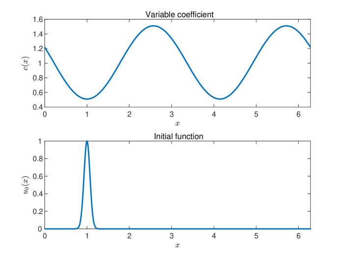
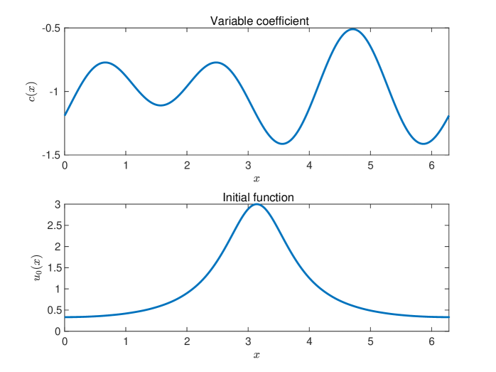
As the first example, we consider the initial-boundary value problem (1) with

$$c(x)=0.51+\sin^{2}(x-1),\quad u_{0}(x)=\sum_{k\in\mathbb{Z}}a_{k}(0)e^{ikx},\quad a_{k}(0)=\frac{1}{20\sqrt{\pi}}e^{-\frac{k^{2}}{400}-ik}.$$

This initial function is an analytic function satisfying $u_{0}(x)\approx e^{-100(x-1)^{2}}$. Because the Fourier coefficients of $e^{-100(x-1)^{2}}$ are

$$\frac{1}{2\pi}\int_{0}^{2\pi}e^{-100(x-1)^{2}}e^{-ikx}dx=\frac{e^{-\frac{k^{2}}{400}-ik}}{40\sqrt{\pi}}\left(\operatorname{erf}\left(\frac{ik+400\pi-200}{20}\right)-\operatorname{erf}\left(\frac{ik-200}{20}\right)\right)~{}(k\in\mathbb{Z}),$$

we approximate the term $\operatorname{erf}\left(\frac{ik+400\pi-200}{20}\right)-\operatorname{erf}\left(\frac{ik-200}{20}\right)$ as $2$, where $\operatorname{erf}(x)=\frac{2}{\sqrt{\pi}}\int_{0}^{x}e^{-s^{2}}ds$. In [30], the function $e^{-100(x-1)^{2}}$ is said that this function is not mathematically periodic, but it is so close to zero at the ends of the interval that it can be regarded as periodic in practice. Then, we set such an initial function that is rigorously periodic and is close to $e^{-100(x-1)^{2}}$. The truncated error of the initial function in (24) is estimated by

(27) $$\left(\sum_{|k|>N}|a_{k}(0)|^{2}\right)^{1/2} =\frac{1}{20\sqrt{\pi}}\left(\sum_{|k|>N}\left|e^{-\frac{k^{2}}{400}}\right|^{2}\right)^{1/2}$$

$$=\frac{1}{10\sqrt{2\pi}}\left(\sum_{k=N+1}^{\infty}\left|e^{-\frac{k^{2}}{400}}\right|^{2}\right)^{1/2}$$

$$\leq\frac{1}{10\sqrt{2\pi}}\left(\int_{N}^{\infty}e^{-\frac{x^{2}}{200}}dx\right)^{1/2}$$

$$=\frac{1}{2}\left(\operatorname{erfc}\left(\frac{N}{10\sqrt{2}}\right)\right)^{1/2},$$

where $\operatorname{erfc}(x)=1-\operatorname{erf}(x)$. Furthermore, the Fourier coefficients of $c(x)$ are given by

$$c_{k}=\begin{cases}-\frac{e^{2i}}{4},&k=-2,\\ 1.01,&k=0,\\ -\frac{e^{-2i}}{4},&k=2,\\ 0,&\mbox{otherwise}.\end{cases}$$

It is shown that the sequence $c=(c_{k})_{k\in\mathbb{Z}}$ satisfies $Bc\in\ell^{1}$ and (6). Theorem 2.8 follows that the operator $A$ defined in (3) generates the $C_{0}$ semigroup of $G(1,\omega)$ class on the sequence space $X$ with

$$\omega=\frac{1}{2}\|Bc\|_{1}=\frac{1}{2}.$$

The profile of the variable coefficient $c(x)$ and that of the initial function $u_{0}(x)$ are displayed in Figure 1.

Figure 1: Profile of the variable coefficient (upper) and that of the initial function (lower) in Example 1.

In Figure 2, we plot the behavior of the numerically computed approximate solution $\tilde{u}$.

Figure 2: Numerically computed approximate solution of (1) in Example 1.

Figure 3 shows rigorous upper bounds of $\|z(0)\|_{X}$ using (24) with (27). A remarkable accuracy can be seen in Figure 3, which illustrates the efficiency of the spectral method.

Figure 3: Error estimates of the initial function $\|z(0)\|_{X}$ in Example 1.

Rigorous upper bounds of (24) with (27) are shown when $N=10,20,\dots,250$. The accuracy of the error estimate is sufficiently small and the rounding errors take over when $N\geq 120$. Furthermore, the decay rate of the estimate looks exponential order, which is called “spectral accuracy” in [30].

Figure 4 also shows rigorous numerical results of the residual estimate discussed in Section 3.1.3. This result implies that the number of Chebyshev basses in order to sufficiently reduce the residual estimate is increasing as $t_{\max}$ getting larger.

Figure 4: Residual estimates $\|r\|_{C((0,t_{\max});X)}$ ($N=120$) in Example 1.

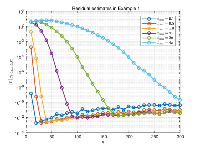
Rigorous upper bounds of the residual estimate (26) are shown when $n=10,20,\dots,300$ varying $t_{\max}=0.1,0.5,1,\pi,2\pi,4\pi$. The accuracy becomes small and the rounding errors take over for large $n$. The decay rate also looks exponential order with respect to $n$. In particular, when one take the sufficiently large number of Chebyshev basses, the accuracy of the residual estimate becomes tiny even if $t_{\max}$ is large.

Consequently, in Table 1, we sum up each numerical result of our verified computing when $t_{\max}=0.1$, $0.5$, $\pi$, $2\pi$, $4\pi$ and $N=120$.

Table 1: Numerical results of verified computing in Example 1.

$t_{\max}$	$N$	$n$	initial error	residual	error	app. time	exec. time	ratio
0.1	120	15	1.888e-16	6.6975e-14	7.0663e-15	0.2258	0.2634	1.166
0.5	120	28	1.888e-16	1.331e-13	7.5849e-14	1.0445	1.0881	1.042
1.0	120	39	1.888e-16	2.0349e-13	2.6433e-13	2.0794	2.1221	1.021
$\pi$	120	97	1.888e-16	7.3368e-13	5.5922e-12	6.8228	6.8702	1.007
$2\pi$	120	182	1.888e-16	1.6846e-12	7.46e-11	13.6139	13.6696	1.004
$4\pi$	120	355	1.888e-16	6.5085e-12	6.9576e-09	27.2039	27.2845	1.003

Here, “initial error”, “residual”, and “error” denote the upper bound of $\|z(0)\|_{X}$, that of the residual $\|r\|_{C((0,t_{\max});X)}$, and that of $\|z\|_{C((0,t_{\max});X)}$ given in Theorem 3.1, respectively. The “app. time” and “exec. time” are results of computational time on the second time scale for getting an approximate solution by ode45 in Chebfun and those of all computational time for our verified computing, respectively. The “ratio” presents an additional ratio of verified computing given by the value of “exec. time” divided by “app. time”. The main feature of these results is the accuracy of the residual estimate, which is remarkably high accurate for verified computing to PDEs. It is worth noting that the rigorous error estimate is still small even if $t_{\max}$ is getting larger. Another feature of the results is the speed of verified numerical computations. In Table 1, we observe that it requires at most tens of percent of additional time with respect to the execute time of the ODE integrator in Chebfun. This indicates that our method of verified computing is executed as fast as (non-rigorous) numerical computations.

4.2 Example 2

The second example is the initial-boundary value problem (1) with

$$c(x)=1+0.49\cos 2x,~{}~{}u_{0}(x)=\frac{3}{5+4\cos x}.$$

The profile of the variable coefficient $c(x)$ and that of the initial function $u_{0}(x)$ are displayed in Figure 5.

Figure 5: Profile of the variable coefficient (upper) and that of the initial function (lower) in Example 2.

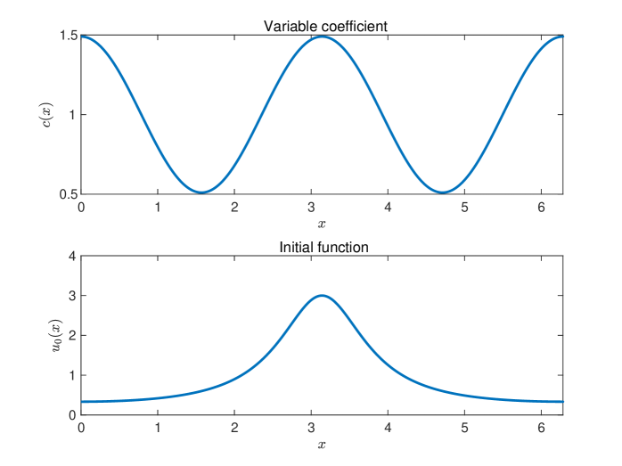
The Fourier coefficients of the initial function are given by $a_{k}(0)=(-2)^{-|k|}$. Because the floating-point number is binary format with base $2$, the rounding error in calculating the coefficients becomes zero. Then, the initial error is only the truncated error. Such a truncated error of the initial function in (24) is estimated by

(28) $$\left(\sum_{|k|>N}|a_{k}(0)|^{2}\right)^{1/2}=\left(2\sum_{k=N+1}^{\infty}\left|(-2)^{-k}\right|^{2}\right)^{1/2}=\sqrt{\frac{2}{3}}\,2^{-N}.$$

Furthermore, the Fourier coefficients of $c(x)$ are given by

$$c_{k}=\begin{cases}\frac{0.49}{2},&k=-2,\\ 1,&k=0,\\ \frac{0.49}{2},&k=2,\\ 0,&\mbox{otherwise}.\end{cases}$$

The sequence $c=(c_{k})_{k\in\mathbb{Z}}$ immediately satisfies $Bc\in\ell^{1}$ and (6). Theorem 2.8 follows that the operator $A$ defined in (3) generates the $C_{0}$ semigroup of $G(1,\omega)$ class on the sequence space $X$ with

$$\omega=\frac{1}{2}\|Bc\|_{1}=0.49.$$

In Figure 6, we plot the behavior of the numerically computed approximate solution $\tilde{u}$.

Figure 6: Numerically computed approximate solution of (1) in Example 2.

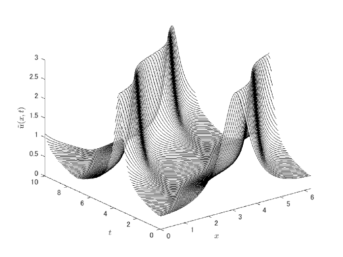
Figure 7 shows rigorous upper bounds of the residual estimate discussed in Section 3.1.3. The results are almost same as that in the previous example. The residual estimate becomes sufficiently small as increasing the number of Chebyshev basses even if $t_{\max}=4\pi(\approx 12.57)$.

Figure 7: Residual estimates $\|r\|_{C((0,t_{\max});X)}$ ($N=150$) in Example 2.

Rigorous upper bounds of the residual estimate (26) are shown when $n=10,20,\dots,300$ varying $t_{\max}=0.1,0.5,1,\pi,2\pi,4\pi$. The decay rate also looks exponential order with respect to $n$.

Table 2 lists the best numerical result of verified computing when $t_{\max}=0.1,~{}0.5,~{}\pi,~{}2\pi,~{}4\pi$.

Table 2: Numerical results of verified computing in Example 2.

$t_{\max}$	$N$	$n$	initial error	residual	error	app. time	exec. time	ratio
0.1	110	13	2.2662e-17	3.1829e-13	3.2645e-14	0.5219	0.5533	1.060
0.5	152	29	1.0806e-23	3.8705e-13	2.1929e-13	3.4671	3.5052	1.011
1.0	194	46	5.1528e-30	6.4904e-13	8.3755e-13	12.7719	12.8210	1.004
$\pi$	223	121	2.2239e-34	2.7793e-12	2.077e-11	48.1160	48.1829	1.001
$2\pi$	190	247	2.0611e-29	8.2819e-12	3.504e-10	74.3893	74.4721	1.001
$4\pi$	200	536	6.441e-31	1.6484e-11	1.5854e-08	166.2447	166.4098	1.001

Here, “best” means that our code returns the smallest rigorous error estimate given in Theorem 3.1. As indicated in Example 1, the high accuracy and high speed of verified numerical computations catch one’s attention to illustrate the efficiency of the method.

4.3 Example 3

For the final example, we consider a slightly more complicated initial-boundary value problem (1) than that in the previous two examples, where

$$c(x)=-1+0.3\sin 3x-0.19\cos 2x,~{}~{}u_{0}(x)=\frac{3}{5+4\cos x}.$$

The profile of the variable coefficient $c(x)$ and that of the initial function $u_{0}(x)$ are displayed in Figure 8.

Figure 8: Profile of the variable coefficient (upper) and that of the initial function (lower) in Example 3.

The truncated error of the initial function in (24) is the same as that in (28). The Fourier coefficients of $c(x)$ are given by

$$c_{k}=\begin{cases}\frac{0.3}{2i},&k=-3,\\ -\frac{0.19}{2},&k=-2,\\ -1,&k=0,\\ -\frac{0.19}{2},&k=2,\\ -\frac{0.3}{2i},&k=3,\\ 0,&\mbox{otherwise}.\end{cases}$$

The sequence $c=(c_{k})_{k\in\mathbb{Z}}$ immediately satisfies $Bc\in\ell^{1}$ and (6). Theorem 2.8 follows that the operator $A$ defined in (3) generates the $C_{0}$ semigroup of $G(1,\omega)$ class on the sequence space $X$ with

$$\omega=\frac{1}{2}\|Bc\|_{1}=0.64.$$

In Figure 9, we plot the behavior of the numerically computed approximate solution $\tilde{u}$.

Figure 9: Numerically computed approximate solution of (1) in Example 3.

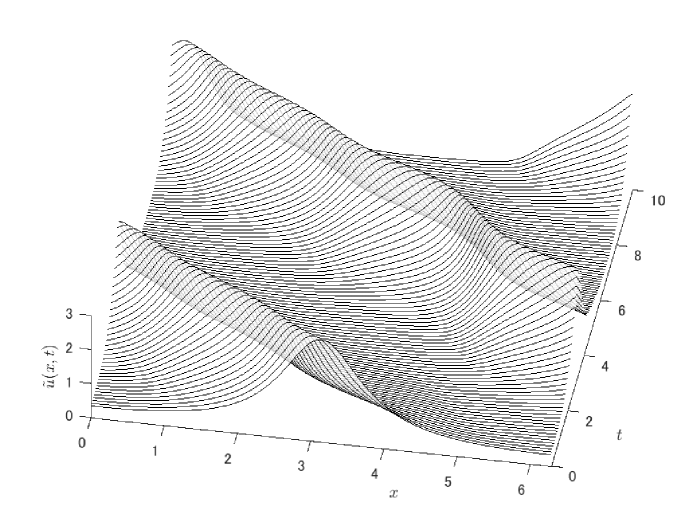
Table 3 lists the best numerical result of verified computing when $t_{\max}=0.1,~{}0.5,~{}\pi,~{}2\pi,~{}4\pi$.

Table 3: Numerical results of verified computing in Example 3.

$t_{\max}$	$N$	$n$	initial error	residual	error	app. time	exec. time	ratio
0.1	130	14	2.2131e-20	4.238e-13	4.3765e-14	0.1897	0.2266	1.195
0.5	87	28	6.5637e-14	3.8734e-13	3.1864e-13	0.5942	0.6274	1.056
1.0	200	40	6.441e-31	5.0248e-13	7.0385e-13	9.3328	9.3987	1.007
$\pi$	160	127	6.7539e-25	1.6567e-12	1.6743e-11	6.6772	6.7346	1.009
$2\pi$	197	251	1.8218e-30	4.8822e-12	4.1781e-10	54.0988	54.2070	1.002
$4\pi$	232	526	9.8282e-36	2.3755e-11	1.1541e-07	156.3342	156.5644	1.001

Our method of verified computing also gives tight error bounds between the exact solution and its numerically computed approximate solution. Moreover, it is executed in high speed. These are benefit of using the spectral method.

Conclusion

In the present paper, we have derived a methodology of verified computing for solutions to 1-dimensional advection equations with variable coefficients based on the Fourier-Chebyshev spectral method. Main contribution of this paper is to provide a method of verified computing using the $C_{0}$ semigroup on the complex sequence space $\ell^{2}$, which comes from the Fourier series of the solution. We have applied the Lumer-Phillips theorem for an operator $A$ generating the $C_{0}$ semigroup on the sequence space. A sufficient condition for the generator of the $C_{0}$ semigroup is shown in Theorem 2.8. In Theorem 3.1, we have introduced the rigorous error estimate between the exact solution and its numerically computed approximate solution. Moreover, numerical results given in Section 4 show that the rigorous error estimate is quite accurate and the computational time is as fast as that of usual numerical computations. In the field of verified numerical computations, the provided methodology is a foundational approach for initial-boundary value problems of hyperbolic PDEs.

We conclude this paper by discussing some potential extensions. Our methodology in the present paper could be extended to mathematical models of nonlinear waves. One example is mathematical models of the traffic stream $\rho_{t}+(\rho u)_{x}=0$, where $\rho$ is the traffic density and $u$ denotes vehicle’s velocity. More generally, the provided method could be extended to rigorously compute solutions to multi-dimensional advection equations so-called Mass transport equation $u_{t}+\nabla\cdot(\bm{v}u)=0$ with a given stationary velocity field $\bm{v}$. Furthermore, a more challenging extension is to rigorously compute solutions of the systems of conservation law $u_{t}+(f(u))_{x}=0$ for an unknown function $u(x,t)$. In all of these extensions, the main difficulty is the loss of smoothness caused by the nonlinearity. When that happens, the spectral method typically fails and so-called Gibbs phenomenon occurs. On the other hand, there is a vast amount of results (cf. [6, Chapter 13]) on the reduction and elimination of the Gibbs phenomenon. Combining with such techniques, we believe that our semigroup approach still works well in the nonlinear problems. One interesting future project could be to apply the present method to the radii-polynomial approach developed in [5, 9, 11] etc. for rigorous spectral methods in nonlinear hyperbolic PDEs.

Acknowledgment. The authors express their sincere gratitude to Dr. M. Sobajima in Tyokyo University of Science for his essential suggestion on generating the $C_{0}$ semigroup on sequence spaces. This work was partially supported by JSPS Grant-in-Aid for Early-Career Scientists, No. 18K13453.

References

- [1] J. Boyd. Chebyshev and Fourier Spectral Methods: Second Revised Edition. Dover Books on Mathematics. Dover Publications, 2013.
- [2] H. Brezis. Functional Analysis, Sobolev Spaces and Partial Differential Equations. Universitext. Springer New York, 2010.
- [3] T. A. Driscoll, N. Hale, and L. N. Trefethen. Chebfun Guide. Pafnuty Publications, 2014.
- [4] L. Evans. Partial Differential Equations. Graduate studies in mathematics. American Mathematical Society, 1998.
- [5] J.-L. Figueras, M. Gameiro, J.-P. Lessard, and R. de la Llave. A framework for the numerical computation and a posteriori verification of invariant objects of evolution equations. SIAM Journal on Applied Dynamical Systems, 16(2):1070–1088, 2017.
- [6] J. S. Hesthaven. Numerical Methods for Conservation Laws. Society for Industrial and Applied Mathematics, Philadelphia, PA, 2017.
- [7] J. S. Hesthaven, S. Gottlieb, and D. Gottlieb. Spectral Methods for Time-Dependent Problems. Cambridge Monographs on Applied and Computational Mathematics. Cambridge University Press, 2007.
- [8] E. Hille. Functional Analysis and Semi-groups. Number 31 in American Mathematical Society: Colloquium publications. American Mathematical Society, 1948.
- [9] A. Hungria, J.-P. Lessard, and J. D. M. James. Rigorous numerics for analytic solutions of differential equations: the radii polynomial approach. Mathematics of Computation, 85:1427–1459, 2016.
- [10] K. Ito and F. Kappel. Evolution Equations and Approximations. Series on Advances in Mathematics for Applied Sciences. World Scientific Publishing Company, 2002.
- [11] J.-P. Lessard and J. D. M. James. Computer assisted fourier analysis in sequence spaces of varying regularity. SIAM Journal on Mathematical Analysis, 49(1):530–561, 2017.
- [12] G. Lumer and R. S. Phillips. Dissipative operators in a Banach space. Pacific Journal of Mathematics, 11(2):679–698, 1961.
- [13] J. Mason and D. Handscomb. Chebyshev Polynomials. Chapman and Hall/CRC, 2002.
- [14] T. Minamoto. Numerical verification of solutions for nonlinear hyperbolic equations. Applied Mathematics Letters, 10(6):91–96, 1997.
- [15] T. Minamoto. Numerical existence and uniqueness proof for solutions of nonlinear hyperbolic equations. Journal of Computational and Applied Mathematics, 135(1):79–90, 2001.
- [16] T. Minamoto. Numerical verification method for solutions of nonlinear hyperbolic equations. In G. Alefeld, J. Rohn, S. Rump, and T. Yamamoto, editors, Symbolic Algebraic Methods and Verification Methods, pages 173–181, Vienna, 2001. Springer Vienna.
- [17] M. Mizuguchi, A. Takayasu, T. Kubo, and S. Oishi. A method of verified computations for solutions to semilinear parabolic equations using semigroup theory. SIAM Journal on Numerical Analysis, 55(2):980–1001, 2017.
- [18] M. Mizuguchi, A. Takayasu, T. Kubo, and S. Oishi. Numerical verification for existence of a global-in-time solution to semilinear parabolic equations. Journal of Computational and Applied Mathematics, 315:1–16, 2017.
- [19] M. T. Nakao. A numerical approach to the proof of existence of solutions for elliptic problems. Japan Journal of Applied Mathematics, 5(2):313, Jun. 1988.
- [20] M. T. Nakao. Numerical verifications of solutions for nonlinear hyperbolic equations. Interval Computations, 4(4):64–77, 1994.
- [21] M. T. Nakao. On verified computations of solutions for nonlinear parabolic problems. Nonlinear Theory and Its Applications, IEICE, 5(3):320–338, 2014.
- [22] M. T. Nakao and Y. Watanabe. Numerical verification methods for solutions of semilinear elliptic boundary value problems. Nonlinear Theory and Its Applications, IEICE, 2(1):2–31, 2011.
- [23] A. Pazy. Semigroups of Linear Operators and Applications to Partial Differential Equations. Springer-Verlag New York, 1983.
- [24] M. Plum. Computer-assisted existence proofs for two-point boundary value problems. Computing, 46(1):19–34, Mar. 1991.
- [25] M. Plum. Existence and multiplicity proofs for semilinear elliptic boundary value problems by computer assistance. Jahresber. Deutsch. Math.-Verein., 110:19–54, 2008.
- [26] S. M. Rump. INTLAB - INTerval LABoratory. In T. Csendes, editor, Developments in Reliable Computing, pages 77–104. Kluwer Academic Publishers, Dordrecht, 1999.
- [27] A. Takayasu, X. Liu, and S. Oishi. Verified computations to semilinear elliptic boundary value problems on arbitrary polygonal domains. Nonlinear Theory and Its Applications, IEICE, 4(1):34–61, 2013.
- [28] A. Takayasu, M. Mizuguchi, T. Kubo, and S. Oishi. Accurate method of verified computing for solutions of semilinear heat equations. Reliable Computing, 25:74–99, 2017.
-
[29]
A. Takayasu, S. Yoon, and Y. Endo.
Codes of “Rigorous numerical computations for 1D advection
equations with variable coefficients”.
http://www.risk.tsukuba.ac.jp/~takitoshi/codes/Rc1Daevc2.zip, 2018. - [30] L. N. Trefethen. Spectral Methods in MATLAB. Society for Industrial and Applied Mathematics, 2000.
- [31] A. Yagi. Abstract Parabolic Evolution Equations and their Applications. Springer-Verlag Berlin Heidelberg, 2010.
- [32] N. Yamamoto. A numerical verification method for solutions of boundary value problems with local uniqueness by Banach’s fixed-point theorem. SIAM Journal on Numerical Analysis, 35(5):2004–2013, 1998.
- [33] K. Yosida. On the differentiability and the representation of one-parameter semi-group of linear operators. Journal of the Mathematical Society of Japan, 1(1):15–21, 09 1948.
- [34] P. Zgliczynski and K. Mischaikow. Rigorous Numerics for Partial Differential Equations: The Kuramoto—Sivashinsky Equation. Foundations of Computational Mathematics, 1(3):255–288, Jul. 2001.