Some Approximation Bounds for Deep Networks

Abstract

In this paper we introduce new bounds on the approximation of functions in deep networks and in doing so introduce some new deep network architectures for function approximation. These results give some theoretical insight into the success of autoencoders and ResNets.

1 Introduction

Deep networks have been shown to be more efficient than shallow for certain classes of problems: periodic functions (Szymanski and McCane, 2014); radially symmetric functions (Eldan and Shamir, 2016); and hierarchial compositional functions (Mhaskar and Poggio, 2016). Other work has shown that deep networks can efficiently represent low-dimensional manifolds (Basri and Jacobs, 2016; Shaham et al., 2016), and Telgarsky (2016) shows that there exist functions which cannot be efficiently represented with shallow networks.

All is not lost for shallow networks however. Mhaskar (1996) gives bounds for the approximation of Sobolev functions using shallow networks and shows that these bounds are tight. There appear to be no similar bounds for deep networks on this class of functions. One might naturally ask if deep networks can approximate this class of functions with similar bounds, or if shallow networks are demonstrably superior in this case. If the former, then one may conclude that a deep network is never worse than a shallow counterpart and hence we should always favour deep networks. If the latter, then choosing a shallow network may often be a good choice. This paper goes some way to answering this question by establishing upper bounds of approximation on some specific deep network architectures.

2 Definitions

We follow many of the conventions of Mhaskar and Poggio (2016).

Definition 1 ($V_{N}$)

The set of all networks of a given kind with complexity N (the number of units in the network).

Definition 2 ($||{f}||_{\infty}$)

Norm of a function. Let $I^{n}=[-1,1]^{n}$ be the unit cube in $n$ dimensions. Let $\mathbb{X}=C(I^{n})$ be the space of all continuous functions on $I^{n}$ with:

$$||{f}||_{\infty}=\max_{x\in I^{n}}|f(x)|.$$ (1)

Definition 3 (Degree of approximation)

If $f$ is the unknown function to be approximated, then the distance between $f$ and an approximating network is:

$$\text{dist}(f,V_{N})=\inf_{P\in V_{N}}||{f-P}||_{\infty}.$$ (2)

Definition 4 ($W^{m,\infty}(I^{n})$)

A Sobolev space. Let $m\geq 1$ be an integer. Let $W^{m,\infty}(I^{n})$be the set of all functions of $n$ variables with continuous partial derivatives of orders up to $m<\infty$ such that:

$$||{f}||_{\infty}+\sum_{1\leq|k|_{1}\leq m}||{\mathcal{D}^{k}}||_{\infty}\leq 1,$$ (3)

where $\mathcal{D}^{k}$ denotes the partial derivative indicated by the multi-integer $k\geq 1$, and $|k|_{1}$ is the sum of the components of $k$.

Definition 5 ($\sigma$)

The transfer function. Let $\sigma:\mathbb{R}\mapsto\mathbb{R}$ be infinitely differentiable, and not a polynomial on any subinterval of $\mathbb{R}$. Further, we restrict ourselves to $\sigma\in W^{m,\infty}(I^{n})$. Many common smooth transfer functions satisfy these conditions including the logistic function, $\tanh$, and softplus.

Definition 6 ($S_{N,n}$)

The class of all shallow networks with $N$ units and $n$ inputs. Let $S_{N,n}$ denote the class of shallow networks with $N$ units of the form:

$$x\mapsto\sum_{k=1}^{N}a_{k}\sigma(\langle w_{k},x\rangle+b_{k})$$ (4)

where $w_{k}\in\mathbb{R}^{n}$, $a_{k},b_{k}\in\mathbb{R}$. The number of trainable parameters in such a network is $(n+2)N$. Since $\sigma\in W^{m,\infty}(I^{n})$, it should be obvious that $S_{N,n}\in W^{m,\infty}(I^{n})$.

In all the deep networks we consider, one neuron in each layer after the first hidden layer is identified as the function approximation neuron. This allows us to progressively approximate the function of interest.

Definition 7 ($R_{N,n,l}$)

The class of input residual networks with $N$ units per layer, where $l$ is the number of layers, and $g_{a,b,n}\in S_{a,n}$ is the $b^{th}$ layer of the network. The first hidden layer of the network receives just the input coordinates. Each subsequent layer has the input coordinates and all the previous layer as input. See Figure 2.

Definition 8 ($D_{N_{l},n,l}$)

The class of cascade residual networks with $N_{l}$ units per layer, where $l$ is the number of layers, and $g_{a,b,n}\in S_{a,n}$ is the $b^{th}$ layer of the network. The first hidden layer of the network receives just the input coordinates. Each subsequent layer has the input coordinates and the function approximation neuron of the previous layer as input. See Figure 1.

Definition 9 ($L_{N_{l}^{\geq},n,l}$)

The class of fully connected layer networks with $N_{l}\geq n$ units per layer. Each layer is fully connected to the next layer except for the function approximation neuron which is connected to the function approximation neuron and final output neuron only. In this case the number of neurons in each layer exceeds the input dimension. See Figure 3.

Definition 10 ($L_{N_{l}^{<},n,l}$)

The class of fully connected layer networks with $N_{l}<n$ units per layer. See Figure 3.

Figure 1: A CascadeResNet . $X_{i}$ are input nodes, $N_{ij}$ are nodes in layer $i$, and $g_{i}$ are the approximation outputs for layer $i$.

Figure 2: An InputResNet . $X_{i}$ are input nodes, $N_{ij}$ are nodes in layer $i$, and $g_{i}$ are the approximation outputs for layer $i$.

Figure 3: A FullyConnectedLayerNet . $X_{i}$ are input nodes, $N_{ij}$ are nodes in layer $i$, and $g_{i}$ are the approximation outputs for layer $i$.

3 Approximation Bounds

We take as our starting point Theorem 2.1 of Mhaskar (1996) also reported as Theorem 2.1(a) in Mhaskar and Poggio (2016) and reproduce it here:

Theorem 1 (Theorem 2.1(a) of Mhaskar and Poggio (2016))

Let $\sigma:\mathbb{R}\mapsto\mathbb{R}$ be infinitely differentiable, and not a polynomial on any subinterval of $\mathbb{R}$. For $f\in W^{m,\infty}(I^{n})$:

$$\text{dist}(f,S_{N,n})\leq cN^{-m/n},$$ (5)

for some constant $c$.

We use the results of Theorem 1 to derive bounds for the deep network architectures defined above in the next three theorems.

Theorem 2 (Cascade Residual Network Approximation)

Let $\sigma:\mathbb{R}\mapsto\mathbb{R}$ be infinitely differentiable, and not a polynomial on any subinterval of $\mathbb{R}$. For $f\in W^{m,\infty}(I^{n})$, and some constant $c$:

$$\text{dist}(f,R_{N,n,l}) \leq c^{l}N_{l}^{-m(ln+1)/(n(n+1))}$$ (6)

Proof 3.1.

From Theorem 1, choose $g_{1}\in S_{N,n}$, so that:

$$||{f-g_{1}}||_{\infty}\leq c_{1}N_{l}^{-m/n}$$ (7)

where $c_{1}$ is some constant. From the first layer, create a new function to approximate:

$$f_{1}=\frac{1}{c_{1}N_{l}^{-m/n}}(f-g_{1})$$ (8)

$f_{1}$ is clearly in $W^{m,\infty}(I^{n})$ and note that $||{f_{1}}||_{\infty}\leq 1$, and therefore can be approximated with another single layer network ($g_{2}$), leading to the following error of approximation:

$$||{f_{1}-g_{2}}||_{\infty} \leq c_{2}N_{l}^{-m/(n+1)}$$ (9)

$$||{\frac{1}{c_{1}N^{-m/n}}(f-g_{1})-g_{2}}||_{\infty} \leq c_{2}N_{l}^{-m/(n+1)}$$ (10)

$$\frac{1}{c_{1}N^{-m/n}}||{f-g_{1}-c_{1}N^{-m/n}g_{2}}||_{\infty} \leq c_{2}N_{l}^{-m/(n+1)}$$ (11)

$$||{f-g_{1}-c_{1}N^{-m/n}g_{2}}||_{\infty} \leq c_{1}c_{2}N_{l}^{-m(2n+1)/(n(n+1))}$$ (12)

Repeat the procedure by creating a new function to approximate:

$$f_{2}=\frac{1}{c_{1}c_{2}N_{l}^{-m(2n+1)/(n(n+1))}}(f-g_{1}-c_{1}N_{l}^{-m/n)}g_{2})$$ (13)

Again $f_{2}\in W^{m,\infty}(I^{n})$ and $||{f_{2}}||_{\infty}\leq 1$. Approximate $f_{2}$ with a further layer ($g_{3}$):

$$||{f_{2}-g_{3}}||_{\infty} \leq c_{3}N_{l}^{-m/(n+1)}$$ (14)

$$||{\frac{1}{c_{1}c_{2}N_{l}^{-m(2n+1)/(n(n+1))}}(f-g_{1}-c_{1}N_{l}^{-m/n}g_{2})-g_{3}}||_{\infty} \leq c_{3}N_{l}^{-m/(n+1)}$$ (15)

$$\frac{1}{c_{1}c_{2}N_{l}^{-m(2n+1)/(n(n+1))}}||{f-g_{1}-c_{1}N_{l}^{-m/n}g_{2}-c_{1}c_{2}N_{l}^{-m(2n+1)/(n(n+1))}g_{3}}||_{\infty} \leq c_{3}N_{l}^{-m/(n+1)}$$ (16)

$$||{f-g_{1}-c_{1}N_{l}^{-m/n}g_{2}-c_{1}c_{2}N_{l}^{-m(2n+1)/(n(n+1))}g_{3}}||_{\infty} \leq c_{1}c_{2}c_{3}N^{-m(3n+1)/(n(n+1))}$$ (17)

A simple inductive argument completes the proof.

Since $cN_{l}^{-m/n}<1$ (because $||{f}||_{\infty}\leq 1$, a constant function approximation would produce an error less than 1), it follows that the network will approximate the function exponentially fast in the number of layers.

Theorem 3 (Fully Connected Layer Network Approximation, $N_{l}\geq n$)

Let $\sigma:\mathbb{R}\mapsto\mathbb{R}$ be infinitely differentiable, and not a polynomial on any subinterval of $\mathbb{R}$. For $f\in W^{m,\infty}(I^{n})$, and some constant $c$:

$$\text{dist}(f,L_{N^{\geq},n,l}) \leq c^{l}N_{l}^{-m(ln+1)/(n(n+1))}$$ (18)

if each layer is an invertible map.

Proof 3.2.

Define $G_{1}:\mathbb{R}^{n}\mapsto\mathbb{R}^{N_{l}}$ as the (invertible) mapping for layer 1, $G_{i>1}:\mathbb{R}^{N_{l}}\mapsto\mathbb{R}^{N_{l}}$ as the (invertible) mapping for layer i excluding the function approximation neuron $g_{i-1}$ (see Figure 3). The input to node $g_{1}$ is $G_{1}(X)$; to $g_{2}$ is $g_{1},(G_{2}\circ G_{1})(X)$; etc. Consider the input to $g_{2}$. Since $G_{1}$ is an invertible map, if necessary, we could construct the input to $g_{2}$ as $(G_{2}^{\prime}\circ G_{1}^{-1}\circ G_{1})(X)=G_{2}^{\prime}(X)$. Since this is identical to the situation in Theorem 2, the same result applies.

The next theorem deals with the case where $N_{l}<n$. However, in this case a continuous invertible mapping is not possible. Instead we project coordinates into a lower dimensional space using a Hilbert curve mapping to maintain locality (nearby points in the lower dimensional space are nearby in the original space). Theoretically, we could do this with no loss of information, but unfortunately, this requires an infinite recursion, and therefore any computational procedure will induce an error in the new coordinates. Nevertheless, this error can be made small with a fixed cost projection.

A Hilbert curve can be defined by the centre coordinates of a hierarchically divided hypercube. See Figure 4 for a 2D example. The curve itself, up to level $k$, can be constructed by recursively subdividing an initial square and creating line segments between appropriate centre points. The Hilbert curve itself is the limiting curve as $k$ goes to infinity and defines a continuous, but non-differentiable, onto mapping from $n$ dimensions to 1 dimension. There are several ways to generate Hilbert curve mappings both from $n$ dimensions to 1, and from 1 to $n$ dimensions. See Lawder (2000) for one efficient method. For level $k$, the maximum difference between a point in $[0,1]^{n}$ and a point on the curve is $\frac{\sqrt{n}}{2^{k+1}}$.

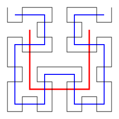
Figure 4: The first 3 levels of a Hilbert curve. From https://commons.wikimedia.org/wiki/File:Hilbert_curve_3.svg, author Geoff Richards.

Theorem 4 (Fully Connected Layer Network Approximation, $N_{l}<n$)

Let $\sigma:\mathbb{R}\mapsto\mathbb{R}$ be infinitely differentiable, and not a polynomial on any subinterval of $\mathbb{R}$. For $f$ Lipschitz with Lipschitz constant $L$, a Hilbert curve transform of level $k$, and some constant $c$:

$$\text{dist}(f,L_{N^{<},n,l}) \leq\frac{L\sqrt{n-N_{l}+1}}{2^{k+1}}+c^{l}N_{l}^{-m(ln+1)/(n(n+1))}$$ (19)

Proof 3.3.

The proof is straightforward. For the coordinate projection from $n$ dimensions to $N_{l}$ dimensions, choose the first $n-N_{l}+1$ dimensions and apply a Hilbert curve transformation. This induces a coordinate error less than $\frac{\sqrt{n-N_{l}+1}}{2^{k+1}}$ and subsequently a function approximation error less than $L\frac{\sqrt{n-N_{l}+1}}{2^{k+1}}$. We then apply Theorem 3 on the remaining $N_{l}$ coordinates along with the triangle inequality to prove the result.

4 Discussion

The constants, $c$, in the theorems pose some difficulty since the errors are exponential in the number of layers ($c^{l}$). It appears to be possible to estimate the size of these constants (Dupont and Scott, 1978, 1980), however the process is not straightforward and we have not attempted to estimate them. Nevertheless these theoretical results provide hints that for more general functions deep networks are never much worse than shallow networks. Given previous results showing that deep networks can be much better than shallow for specific function classes, it follows that there is little to lose in always choosing deep architectures (modulo the difficulties in learning deep networks).

These theoretical results also point toward layer-wise learning algorithms that reduce error exponentially fast in a manner that is somewhat analagous to AdaBoost like algorithms. We are currently investigating the practical implications of such algorithms.

For layer-wise learning of fully connected networks, Theorem 3 suggests that requiring invertible maps might be important. This might explain some of the success of autoencoders. Although Theorem 4 suggests that non-invertible maps might be able to achieve similar results, via space-filling curve mappings, it remains to be seen if such a scheme would be practical.

More recently, ResNets (He et al., 2016; Szegedy et al., 2017) of various types have been shown to outperform non-ResNet architectures with the most common argument given for their success being that it is easier for the gradients to propagate back to the inputs during learning. Theorem 2 and 3 together suggest a second reason may be that it is also easier to approximate residual functions if layers are skipped as there is no requirement that the layer mapping be invertible.

References

- Basri and Jacobs (2016) Ronen Basri and David Jacobs. Efficient representation of low-dimensional manifolds using deep networks. arXiv preprint arXiv: 1602.04723, 2016.
- Dupont and Scott (1978) Todd Dupont and Ridgway Scott. Constructive polynomial approximation in sobolev spaces. Recent advances in numerical analysis. Boor C. and Golub G., Eds, pages 31–44, 1978.
- Dupont and Scott (1980) Todd Dupont and Ridgway Scott. Polynomial approximation of functions in sobolev spaces. Mathematics of Computation, 34(150):441–463, 1980.
- Eldan and Shamir (2016) Ronen Eldan and Ohad Shamir. The power of depth for feedforward neural networks. JMLR: Workshop and Conference Proceedings, 49:1–34, 2016.
- He et al. (2016) Kaiming He, Xiangyu Zhang, Shaoqing Ren, and Jian Sun. Deep residual learning for image recognition. In Proceedings of the IEEE conference on computer vision and pattern recognition, pages 770–778, 2016.
- Lawder (2000) Jonathan K. Lawder. Calculation of mappings between one and n-dimensional values using the hilbert space-filling curve. Technical Report Research Report BBKCS-00-01, School of Computer Science and Information Systems, Birkbeck College, 2000.
- Mhaskar (1996) Hrushikesh N Mhaskar. Neural networks for optimal approximation of smooth and analytic functions. Neural Computation, 8:164–177, 1996.
- Mhaskar and Poggio (2016) Hrushikesh N Mhaskar and Tomaso Poggio. Deep vs. shallow networks: An approximation theory perspective. Analysis and Applications, 14(06):829–848, 2016.
- Shaham et al. (2016) Uri Shaham, Alexander Cloninger, and Ronald R Coifman. Provable approximation properties for deep neural networks. Applied and Computational Harmonic Analysis, 2016.
- Szegedy et al. (2017) Christian Szegedy, Sergey Ioffe, Vincent Vanhoucke, and Alexander A Alemi. Inception-v4, inception-resnet and the impact of residual connections on learning. In AAAI, volume 4, page 12, 2017.
- Szymanski and McCane (2014) Lech Szymanski and Brendan McCane. Deep networks are effective encoders of periodicity. Neural Networks and Learning Systems, IEEE Transactions on, 25(10):1816–1827, 2014.
- Telgarsky (2016) Matus Telgarsky. Benefits of depth in neural networks. JMLR: Workshop and Conference Proceedings, 49:1–23, 2016.