Abstract

We introduce a numerical variational method based on the Rayleigh-Ritz optimization principle for predicting two-dimensional self-trapped beams in nonlinear media. This technique overcomes the limitation of the traditional variational approximation in performing analytical Lagrangian integration and differentiation. Approximate soliton solutions of a generalized nonlinear Schrödinger equation are obtained, demonstrating robustness of the beams of various types (fundamental, vortices, multipoles, azimuthons) in the course of their propagation. The algorithm offers possibilities to produce more sophisticated soliton profiles in general nonlinear models.

OCIS codes: (000.4430) Numerical approximation and analysis; (190.6135) Spatial solitons.

1 Introduction

Self-trapped beams in nonlinear media, alias optical spatial solitons, have long been the subject of intensive studies, promising new physical effects and potential application to optic-communication systems and photonic technologies [1, 2]. Common theoretical models for producing optical solitons rely on the use of generalized nonlinear Schrödinger equations (GNLSEs), which usually do not admit exact solutions. Analytical techniques, such as the inverse scattering method [3] and Bäcklund transform [4], apply only to exceptional integrable systems. Numerical methods for generating soliton solutions, including the standard relaxation algorithm and conjugate gradient method [5] are very useful, but they do not always provide sufficient insight. In particular, an iterative method was developed for finding numerical eigenfunctions and eigenvalues corresponding to soliton solutions of the nonlinear Schrödinger equation, and applied it in a variety of cases (see [6, 7]). Similar to the situation with the standard relaxation algorithm, the success of the iterative method depends on the appropriate choice of the initial guess [8]. To provide deeper understanding of nonlinear systems, approximate semi-analytical methods have been developed, the most useful one being, arguably, the variational approximation (VA) based on the Rayleigh-Ritz optimization of a trial function, alias ansatz, that was introduced in the context of pulse propagation in nonlinear fiber optics in the seminal paper by Anderson [9] (see also works [10] and [11]). The VA makes it possible to predict nonlinear modes with different degrees of accuracy, depending on the choice of the underlying ansatz [12], in diverse nonlinear systems. These include, in particular, photonic lattices in nonlinear media, induced by non-diffracting beams [13], dissipative media [14, 15], Bose-Einstein condensates [16, 17], parity-time-symmetric lattices [18], dynamics of spatio-temporal solitons in a periodic medium [19], and even the prediction of complex hopfion modes with two topological charges (twisted vortex ring) [20]. The VA was also applied to nonlocal GNLSEs [21, 22]. Furthermore, predicted the approximate solutions predicted by the VA can be used in the context of the above-mentioned numerical methods, as an appropriate initial distribution which accelerates the convergence to numerically exact solutions.

Coming along with assets of the VA are its technical limitations, as in many cases it may be problematic to perform analytical integration of the underlying Lagrangian with the substitution of the chosen ansatz, and subsequent differentiation with respect to free parameters, aiming to derive the Euler-Lagrange (EL) equations. In this work, we present an algorithm that permits a full numerical treatment of the VA based on the Rayleigh-Ritz optimization, overcoming its intrinsic limitations. In fact, the development of such fully numerical approach is natural, as, in most cases, the EL equations are solved numerically, anyway. In particular, we use the numerically implemented VA to obtain approximate solutions for rotary multipole modes, as well as vorticity-carrying ring-shaped solitons, in the context of the GNLSEs with various nonlinear terms, cf. Ref. [20].

2 Theoretical framework

2.1 Lagrangian

Evolution equations for complex amplitude $\Psi$ of the optical field are derived from action

$$S=\int\int\mathcal{L}{d}t{d}\mathbf{r}=\int L{d}t,$$ (1)

where $t$ is the evolution variable, $\mathbf{r}$ a set of transverse coordinates, $\mathcal{L}$ the Lagrangian density and $L=\int\mathcal{L}d\mathbf{r}$ the full Lagrangian. As we search for soliton solutions, the field and its derivatives must vanish at boundaries of the integration domain, which emulate the spatial infinity in terms of the numerical solution. The respective EL equation follows from the action-minimum principle, $\delta S/\delta\Psi^{\ast}=0$, i.e.,

$$\frac{d}{dt}\left(\frac{\partial\mathcal{L}}{\partial\Psi_{t}^{\ast}}\right)+\sum_{r_{i}=x,y,z}\frac{d}{dr_{i}}\left(\frac{\partial\mathcal{L}}{\partial\Psi_{r_{i}}^{\ast}}\right)-\frac{\partial\mathcal{L}}{\partial\Psi^{\ast}}=0,$$ (2)

where $\Psi^{\ast}$ is the complex conjugate $\Psi$. In particular, the GNLSE, in the form of

$$i\partial_{t}\Psi+\nabla^{2}\Psi+N(|\Psi|^{2},\mathbf{r})\Psi=0,$$ (3)

with the nonlinear part $N(|\Psi|^{2},\mathbf{r})\Psi$ [23], is generated by

$$\mathcal{L}=\frac{i}{2}(\Psi\partial_{t}\Psi^{\ast}-\Psi^{\ast}\partial_{t}\Psi)+|\nabla\Psi|^{2}+\mathcal{NL}(|\Psi|^{2},\mathbf{r}),$$ (4)

where $\mathcal{NL}(|\Psi|^{2},\mathbf{r})$ is the anharmonic term in the Lagrangian density which gives rise to $N(|\Psi|^{2},\mathbf{r})\Psi$ in the GNLSE.

2.2 Numerical variational method

We start by defining vectors $\mathbf{A}=(A_{1},A_{2},...,A_{n})$ and $\nabla_{\mathbf{A}}L_{\mathbf{(A)}}=(\partial_{A_{1}}L_{\mathbf{(A)}},\partial_{A_{2}}L_{\mathbf{(A)}},...,\partial_{A_{n}}L_{\mathbf{(A)}})$, where $A_{1}$, $A_{2}$,…, $A_{n}$ are variational parameters, such as an amplitude, beam’s width, frequency chirp, etc. We adopt ansatz $\Psi_{(\mathbf{r},\mathbf{A})}$, followed by the integration of $\mathcal{L}$ to produce the respective effective Lagrangian, $L_{\mathbf{(A)}}$, as a function of variables $A_{n}$. As we aim to find solutions for self-trapped beams, we adopt zero boundary conditions at boundaries of the numerical-integration domain. The variation of $L_{\mathbf{(A)}}$ gives rise to the system of the EL equations:

$$\frac{d}{dt}\left(\frac{\partial L_{\mathbf{(A)}}}{\partial\left(dA_{n}/dt\right)}\right)-\frac{\partial L_{\mathbf{(A)}}}{\partial A_{n}}=0\ ,$$ (5)

whose stationary version can be written as $\nabla_{\mathbf{A}}L_{(\mathbf{A})}=0$, with $\nabla_{\mathbf{A}}$ standing for the set of the derivatives with respect to $A_{n}$. Generally, the stationary EL equations cannot be solved analytically, therefore we apply the standard Newton-Raphson multi-variable method, with the Jacobian replaced by the Hessian matrix,

$$HL_{(\mathbf{A})}=\begin{bmatrix}\partial^{2}_{A_{1}}L_{\mathbf{(A)}}&\partial_{A_{2}}\partial_{A_{1}}L_{\mathbf{(A)}}&\dots&\partial_{A_{n}}\partial_{A_{1}}L_{\mathbf{(A)}}\\ \partial_{A_{1}}\partial_{A_{2}}L_{\mathbf{(A)}}&\partial^{2}_{A_{2}}L_{\mathbf{(A)}}&\dots&\partial_{A_{n}}\partial_{A_{2}}L_{\mathbf{(A)}}\\ \dots&\dots&\dots&\dots\\ \partial_{A_{1}}\partial_{A_{n}}L_{\mathbf{(A)}}&\partial_{A_{2}}\partial_{A_{n}}L_{\mathbf{(A)}}&\dots&\partial^{2}_{A_{n}}L_{\mathbf{(A)}}\end{bmatrix}.$$ (6)

In the framework of this method, an the iterative search for the solution is carried out as

$$\mathbf{A}^{(i+1)}=\mathbf{A}^{(i)}-HL_{\mathbf{(A)}}^{-1}\cdot\nabla_{\mathbf{A}}L_{(\mathbf{A})},$$ (7)

starting with an initial guess.

However, the substitution of necessarily complex ansätze in Lagrangians of many nonlinear models leads to analytically intractable integrals. Thus, neither $L_{\mathbf{(A)}}$ nor $\nabla_{\mathbf{A}}L_{\mathbf{(A)}}$ or $HL_{\mathbf{(A)}}$ may be known in an explicit analytical form. This difficulty is exacerbated by working with multidimensional settings and using, if necessary, involved coordinate systems. In this work, we develop a way to overcome this limitation, noting that, to produce $\nabla_{\mathbf{A}}L_{\mathbf{(A)}}$ and $HL_{\mathbf{(A)}}$, which are needed to apply the Newton-Raphson method, one can numerically calculate $L_{(\mathbf{A})}$ at multiple points in the space of variables $A_{n}$, separated by small finite values $\Delta A_{n}$. In particular, the derivatives can be computed as

$$\frac{\partial L_{\mathbf{(A)}}}{\partial A_{n}}=\int\frac{\partial\mathcal{L_{(\mathbf{A})}}}{\partial A_{n}}d\mathbf{r}\approx\int\frac{\mathcal{L}_{(\mathbf{A}+\Delta A_{n})}-\mathcal{L}_{(\mathbf{A}-\Delta A_{n})}}{2\Delta A_{n}}d\mathbf{r}=\frac{L_{(\mathbf{A}+\Delta A_{n})}-L_{(\mathbf{A}-\Delta A_{n})}}{2\Delta A_{n}},$$ (8)

and, similarly,

$$\frac{\partial^{2}L_{\mathbf{(A)}}}{\partial A_{n}\partial A_{m}}\approx\frac{L_{(\mathbf{A}+\Delta A_{n}/2+\Delta A_{m}/2)}-L_{(\mathbf{A}-\Delta A_{n}/2+\Delta A_{m}/2)}-L_{(\mathbf{A}+\Delta A_{n}/2-\Delta A_{m}/2)}+L_{(\mathbf{A}-\Delta A_{n}/2-\Delta A_{m}/2)}}{\Delta A_{n}\Delta A_{m}}.$$ (9)

Note that each step in this procedure can be done numerically. While there is freedom in the choice of $\Delta A_{n}$, it is reasonable to select their size smaller than an estimated solution for $A_{n}$ by at least three orders of magnitude. Thus, the algorithm can be summarized as follows:

• Calculate $\nabla_{\mathbf{A}}L_{\mathbf{(A)}}$ and $HL_{\mathbf{(A)}}$ numerically with the help of Eqs. (8) and (9), respectively. Because $HL_{\mathbf{(A)}}$ is a $n\times n$ symmetric matrix, only $n(n+1)/2$ different elements need to be actually calculated.

• Compute new $\mathbf{A}$ according to Eq. (7).

• Iterate the two previous steps until achieving specified tolerance for the convergence of $\mathbf{A}$.

A disadvantage of this algorithm is that the trivial zero solution also satisfies the optimization procedure, hence the iterations may converge to zero in some cases. A simple but effective way to avoid this is to select a new starting point with larger values of $A_{n}$. It is also worthy to note that, in the case of multistability, the algorithm can find different coexisting solutions, the convergence to a specific one depending on the choice of the initial guess.

3 Numerical results for self-trapped modes

Here we report results obtained for the GNLSEs generated by the Lagrangian with anharmonic terms displayed in Table 1. We start by looking for solutions for spatial solitons, in the form of

$$\Psi(x,y,z)=\psi(\mathbf{r})e^{i\lambda z},$$ (10)

where $\mathbf{r}=\left\{x,y\right\}$ are the transverse spatial coordinates, longitudinal coordinate $z$ is the evolution variable, which replaces $t$ in the outline of the variational method presented above, and $\lambda$ is a real propagation constant. The substitution of this waveform simplifies GNLSE (3) and Lagrangian (4),

$$-\lambda\psi(\mathbf{r})+\nabla_{\perp}^{2}\psi(\mathbf{r})+N(|\psi|^{2},\mathbf{r})\psi(\textbf{r})=0,$$ (11)

$$\mathcal{L}=\lambda|\psi|^{2}+|\nabla_{\perp}\psi|^{2}+\mathcal{NL}(|\psi|^{2},\mathbf{r}).$$ (12)

The iterative procedure for the solution of the optimization problem does not provide the conservation of the dynamical invariants, viz., the norm and Hamiltonian. However, this fact does not invalidate the applicability of the procedure, similarly to the well-known imaginary-time integration method, which provides correct stationary solutions, although the Hamiltonian is not conserved in the course of the solution [24, 25] .

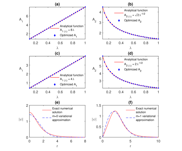
Fig. 1: The amplitude (a) and beam’s width (b), predicted by the numerical variational procedure for the fundamental soliton ($m=0$), compared to the results of the analytical variational approximation (see the text). The maximum relative differences for parameters $A_{1}$ and $A_{2}$ are $e_{A_{1}}=1.72\times 10^{-8}\ \%$ and $e_{A_{2}}=2.40\times 10^{-8}\ \%$ . The same comparison for the amplitude (c) and width (d) of the vortex beam with $m=1$ in the Kerr medium, with maximum relative differences $e_{A_{1}}=2.17\times 10^{-7}\ \%$ and $e_{A_{2}}=1.65\times 10^{-7}\ \%$. Comparison between the exact soliton shape and the variationally obtained using Eq. (7) for fundamental (e) and single vortex soliton (f), in both cases $\lambda=0.5$.

In this work, we focus on the optimization of the following generalized vortex ansatz with integer topological charge $m$ in two-dimensional GNLSEs including anharmonic terms listed in Table 1:

$$\psi(\mathbf{r})=A_{1}^{(m+1)/2}\exp\left[-\left(x/A_{2}\right)^{2}-\left(y/A_{3}\right)^{2}\right]$$

$$\times\left[(\cos^{2}\epsilon)~{}x^{2}+(\sin^{2}\epsilon)~{}y^{2}\right]^{m/2}\left[(\cos\delta)\cos(m\theta)+i~{}\left(\sin\delta\right)\sin(m\theta)\right],$$ (13)

$\theta\equiv\arctan(y/x)$ being the angular coordinate. The ansatz may be construed as either an asymmetric azimuthon [26] or ellipticon [27]. Here, $A_{1}$ represents the amplitude of the anisotropic beam, while $A_{2}$ and $A_{3}$ determine its width, $A_{2}=A_{3}$ corresponding to the isotropic one. Parameters $\epsilon$ and $\delta$ additionally control the beam’s asymmetry and its phase structure. In particular, for $\epsilon=\delta=\pi/4$ the ansatz reduces to a standard vortex beam, while at $\delta=0$ it is reduced to a multi-pole beam.

Generic results can be adequately presented for propagation constant $\lambda=1/2$ in Eq. (10) and values of parameters $s=0.05$ and $k=5$, $p=30$ in Lagrangian terms (15) and (16), respectively, unless specified otherwise.

First, we reproduce known results produced by the VA for the fundamental and first-order vortex solitons in the Kerr medium, corresponding to Eq. (14), based on normalized ansatz $\psi=2^{-(m+1)/2}A_{1}^{(m+1)/2}\exp\left[-(r/A_{2})^{2}\right]r^{m}\exp(im\theta)$ [28]. With this ansatz, the analytical VA yields $A_{1}=8\lambda$ and $A_{2}=\sqrt{2/\lambda}$ for $m=0$, and $A_{1}=4\lambda$ and $A_{2}=2/\sqrt{\lambda}$ for $m=1$. Using the present algorithm leads to complete agreement with these results, as shown in Fig. 1, with relative errors $<3\times 10^{-7}\%$. Each of these sets of the results can be generated by a standard computer in less than a minute. The general agreement between the exact soliton shape and the solution obtained by using the numerical variational approach is good, as is evident from Fig. 1(e) and Fig. 1(f) for the fundamental and single vortex soliton, respectively. In principle, more sophisticated ansätze may provide closer agreement with numerically exact results, but in this work we focus on the basic results produced by the relatively simple ansatz.

Next, we proceed to demonstrate the utility of the algorithm for more complex nonlinear media. We use the combination of the Kerr and first-order Bessel-lattice terms, that is, the sum of terms given  by Eqs. (14) and (16) . We test the utility of the algorithm by comparing its predictions with simulations, using the standard split-step Fourier-transform algorithm and presenting the evolution of the intensity profile, $|\psi|^{2}$, for a certain size of the transverse display area (TDA).

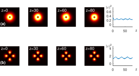
Fig. 2: Simulated propagation in the medium with the combined nonlinearity corresponding to Eq. (14) + Eq. (16), initiated by inputs produced by the numerically implemented variational approximation. (a) The vortex soliton with topological charge $m=1$ with $\mathbf{A_{1,2,3}}=(0.7830,2.7903,2.7903)$ and TDA $15\times 15$. (b) The propagation of the quadrupole soliton in the medium with the combined nonlinearity corresponding to Eq. (14) + Eq. (16), with $\mathbf{A_{1,2,3}}=(0.5767,3.4560,3.4560)$ and TDA $20\times 20$. The peak-intensity evolution is shown in the right-hand column.

Figure 2 (a) displays the numerically simulated propagation of the isotropic vortex soliton with $m=1$, starting from the input predicted by the numerically implemented VA. Note that, while the direct simulation does not preserve a completely invariant shape of the vortex beam, the VA provides a reasonable prediction. It is relevant to mention that the simulations do not include initially imposed azimuthal perturbations, which may lead to breakup of the vortex ring due the azimuthal instability [29].

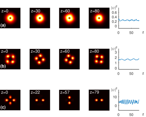
Fig. 3: The same as in Fig. 2, but under the action of the combined nonlinearity given by Eq. (15) + Eq. (16). (a) The vortex with $m=1$, $\mathbf{A_{1,2,3}}=(0.7860,2.7915,2.7915)$, and TDA $15\times 15$. (b) The azimuthon with $m=2$, $\delta=\pi/3$, $\mathbf{A_{1,2,3}}=(0.63574,3.4760,3.4760)$, and TDA $20\times 20$. (c) The asymmetric quadrupole with $s=0.2$, $\lambda=0.8$, $\epsilon=5\pi/16$, $\mathbf{A_{1,2,3}}=(1.0334,3.4235,2.4701)$, and TDA $20\times 20$.

Then, we optimize a quadrupole soliton beam. The simulated propagation is displayed in Fig. 2(b), where the persistence of the VA-predicted shape is obvious. Note that the usual form of the VA cannot be applied in this case, because of its complexity. Further, we proceed to self-trapped beams supported by a combination of the saturable nonlinearity and the first-order Bessel-lattice term, i.e., Eq. (15) + Eq. (16), for three different ansätze: the vortex beam with $m=1$, the azimuthon with $m=2$, and finally, an the elliptic quadrupole. The two former ansätze carry the orbital angular momentum due to their phase structure, which drives their clockwise rotation in the course of the propagation, while preserving the overall intensity shape, as shown in Fig. 3(a) and Fig. 3(b). It is worthy to note that, in the pure saturable medium, an attempt to produce asymmetric quadrupoles by means of the VA optimization does not produce any robust mode, but, if the Bessel term (16) is added, the quadrupole develops into a noteworthy stable dynamical regime of periodic transitions between vertical and horizontal dipole modes, as shown in Fig. 3(c).

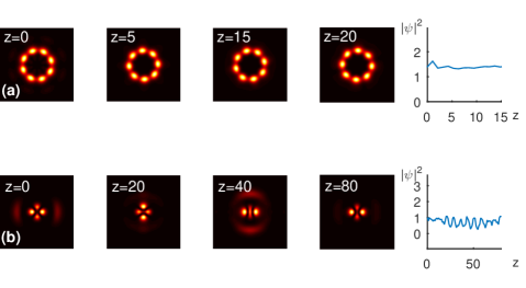
Fig. 4: The same as in Fig. 2, but in the medium with the combination of the nonlinear terms corresponding to the combination of Eqs. (15) + (16), with $s=0.05$, $p=15$ and $k=1$. (a) The fourth-order azimuthon with $\delta=\pi/3$, $\mathbf{A_{1,2,3}}=(0.4216,2.8725,2.8725)$, and TDA $20\times 20$. (b) The asymmetric quadrupole with $\epsilon=5\pi/16$, $\mathbf{A_{1,2,3}}=(1.2722,2.2057,1.3310)$, and TDA $15\times 15$.

Finally, we address the propagation of an azimuthon with $m=4$ and asymmetric quadrupole, under the combined action of the saturable nonlinearity and zeroth-order Bessel lattice, as shown in Fig. 4(a) and Fig. 4(b), respectively. The orbital angular momentum of the modes drives their rotation in the course of the propagation. In particular, the former pattern is predicted in quite a robust form, while the latter one is transformed into the above-mentioned regime of periodic transitions between vertical and horizontal dipole modes. Additional results produced by the general ansatz given by Eq. (13) and the VA outlined above, in the combination with direct simulations, will be reported elsewhere.

Table 1: Anharmonic terms in the Lagrangian

Kerr	$$\mathcal{NL}(|\psi|^{2},\textbf{r})=-1/2|\psi|^{4},$$ (14)
Saturation	$$\mathcal{NL}(|\psi|^{2},\textbf{r})=(\ln(s|\psi|^{2}+1)-s|\psi|^{2})/s^{2},$$ (15)
$n$-th order Bessel lattice	$$\mathcal{NL}(|\psi|^{2},\textbf{r})=-p\left[J_{n}{\ (k\sqrt{x^{2}+y^{2}})}\right]^{2}|\psi|^{2}.\vspace{-2cm}$$ (16)

4 Conclusion

In this work we report an efficient algorithm for full numerical treatment of the variational method predicting two-dimensional solitons of GNLSE (generalized nonlinear Schrödinger equation) with various nonlinear terms, which arise in nonlinear optics. A general class of the solitons is considered, including vortices, multipoles, and azimuthons. The method predicts solutions for the self-trapped beams which demonstrate robust propagation in direct simulations. Further work with the use of the algorithm is expected, making use of more complex flexible ansätze, which should improve the accuracy (making the calculations more complex, which is not a critical problem for the numerically implemented algorithm). In particular, it is planned to apply the VA to models of nonlocal nonlinear media, where the Lagrangian integrals become quite difficult for analytical treatment. Another promising direction is application of the algorithm to three-dimensional settings, where the analytical work is hard too.

Funding

Consejo Nacional de Ciencia y Tecnología (CONACYT) (243284); National Science Foundation (NSF) and Binational (US-Israel) Science Foundation (2015616); Israel Science Foundation (1286/17).