On localizing and concentrating electromagnetic fields

Abstract.

We consider field localizing and concentration of electromagnetic waves governed by the time-harmonic anisotropic Maxwell system in a bounded domain. It is shown that there always exist certain boundary inputs which can generate electromagnetic fields with energy localized/concentrated in a given subdomain while nearly vanishing in another given subdomain. The theoretical results may have potential applications in telecommunication, inductive charging and medical therapy. We also derive a related Runge approximation result for the time-harmonic anisotropic Maxwell system with partial boundary data.

Keywords. electromagnetic waves, localizing and concentration, anisotropic Maxwell system, Runge approximation, partial data

Mathematics Subject Classification (2010): Primary 35Q61; Secondary 78A25, 78A45

1. Introduction

1.1. Background and motivation

The electromagnetic (EM) phenomena are ubiquitous and they lie at the heart of many scientific and technological applications including radar and sonar, geophysical exploration, medical imaging, information processing and communication. In this paper, we are mainly concerned with the mathematical study of field localizing and concentration of electromagnetic waves governed by the time-harmonic Maxwell system in a bounded anisotropic medium. More specifically, we show that there always exist certain boundary inputs which can generate the desired electromagnetic fields that are localized/concentrated in a given subdomain while nearly vanishing in another given subdomain.

The localizing and concentration of electromagnetic fields can have many potential applications. In telecommunication [43], one common means of transmitting information between communication participants is via the electromagnetic radiation. In a certain practical scenario, say the secure communication, one may intend the information to be transmitted mainly to a partner located at a certain region, while avoid the transmission to another region. Clearly, if the information is encoded into the electromagnetic waves that are localized and concentrated in the region where the partner is located while are nearly vanishing in the undesired region, then one can achieve the expected telecommunication effect. In the setup of our proposed study, one can easily obtain the aforementioned communication effect, in particular if the communication participants transmit and receive information on some surface patches.

Concentrating electromagnetic fields can also be useful in inductive charging, also known as wireless charging or cordless charging [42], which is an emerging technology that can have significant impact on the real life. It uses electromagnetic fields to transfer energy between two objects through electromagnetic induction. Clearly, the energy transfer would be more efficient and effective if the corresponding electromagnetic fields are concentrated around the charging station. The localizing of electromagnetic fields can also have potential application in electromagnetic therapy. Though it is mainly considered to be pseudoscientific with no affirmative evidence, the electromagnetic therapy has been widely practiced which claims to treat disease by applying electromagnetic radiation to the body. If the electromagnetic therapy shall be proven to be effective, then through the use of certain purposely designed sources, one can generate electromagnetic fields that are concentrated around the diseased area.

The above conceptual and potential applications make the study of field concentration and localizing much appealing. Nevertheless, it is emphasized that in the current article, we are mainly concerned with the mathematical and theoretical study. We achieve some substantial progress on this interesting topic, though the corresponding study is by no means complete. It is also interesting to note that the localizing of resonant electromagnetic fields has been used to produce invisibility cloaking and has received significant attention in the literature in recent years [2, 3, 6, 30, 33, 36]. The corresponding study is mainly based on the use of plasmonic materials to induce the so-called anomalous localized resonance.

Our mathematical argument for proving the existence of the localized and concentrated electromagnetic fields is mainly based on combining the unique continuation property for the anisotropic Maxwell system with a functional analytic duality argument developed in [12]. By a similar argument, we also obtain a related Runge approximation property.

The use of blow up solutions has a long tradition in the study of inverse boundary value problems, cf. [1, 25, 26, 27] for early seminal works on this topic. Moreover, the combination of localized fields and monotonicity relations have led to the development of monotonicity-based methods for obstacle/inclusion detection, cf. [39, 22] for the origins and mathematical justification of this approach, [5, 7, 9, 10, 11, 21, 16, 17, 18, 19, 23, 32, 38, 40, 41, 44] for further recent contributions, and the recent works [20, 13] for the Helmholtz equation. Theoretical uniqueness results for inverse coefficient problems have also been obtained by this approach in [4, 14, 15, 21, 24]).

In this work, we show the existence of localized electromagnetic fields for the more challenging case of time-harmonic anisotropic Maxwell system with partial data. We also derive a Runge approximation result, that shows that every solution in a subdomain can be approximately well by a solution on the whole domain. In that context let us note the famous equivalence theorem from Peter Lax [28]: the weak unique continuation property is equivalent to the Runge approximation property for the second order elliptic equation. In our study, we affirmatively verify this property still holds for the anisotropic Maxwell system.

The rest of the present section is devoted to the mathematical description of the setup of our study and the statement of the main result.

1.2. Mathematical setup and statement of the main result

Let $\Omega$ be a simply connected domain in $\mathbb{R}^{3}$ with a Lipschitz connected boundary $\partial\Omega$. Let $\epsilon=(\epsilon_{ij})_{1\leq i,j\leq 3}$ and $\mu=(\mu_{ij})_{1\leq i,j\leq 3}$ be two $3\times 3$ real matrix-valued functions satisfying

• Strong ellipticity: There exist constants $\mu_{0}>0$ and $\epsilon_{0}>0$ verifying

  $$\begin{cases}\mu_{0}|\xi|^{2}\leq\sum_{i,j=1}^{3}\mu_{ij}(x)\xi_{i}\xi_{j}\leq\mu_{0}^{-1}|\xi|^{2},\\ \epsilon_{0}|\xi|^{2}\leq\sum_{i,j=1}^{3}\epsilon_{ij}(x)\xi_{i}\xi_{j}\leq\epsilon_{0}^{-1}|\xi|^{2},\end{cases}\mbox{ for any }x\in\Omega\text{ and }\xi\in\mathbb{R}^{3}.$$ (1.1)

• Smoothness: $\epsilon$ and $\mu$ are piecewise Lipschitz continuous matrix-valued functions defined in $\Omega$.

• Symmetry: $\epsilon$ and $\mu$ are symmetric matrices, that is, $\epsilon_{ij}=\epsilon_{ji}$ and $\mu_{ij}=\mu_{ji}$ for all $1\leq i,j\leq 3$.

The functions $\epsilon$ and $\mu$, respectively, signify the electric permittivity and magnetic permeability of the medium in $\Omega$. Consider the time-harmonic electromagnetic wave propagation in $\Omega$. With the $e^{ikt}$ time-harmonic convention assumed, we let $E(x)$ and $H(x)$, respectively, denote the electric and magnetic fields. Here, $k\in\mathbb{R}_{+}$ signifies a wavenumber. Then the electromagnetic wave propagation is governed by the following Maxwell system,

$$\begin{cases}\nabla\times E-ik\mu H=0&\mbox{ in }\Omega,\\ \nabla\times H+ik\epsilon E=0&\mbox{ in }\Omega,\\ \nu\times E=\begin{cases}f&\mbox{ on }\Gamma\\ 0&\mbox{ otherwise}\end{cases}&\mbox{ on }\partial\Omega,\end{cases}$$ (1.2)

where $\Gamma$ is an arbitrary nonempty relative open subset of $\partial\Omega$ and $\nu$ is the unit outer normal vector on $\partial\Omega$. It is assumed that $k>0$ is not an eigenvalue (or non-resonance, see Section 2) for (1.2) and $f\in C^{\infty}_{c}(\Gamma)$ throughout this paper.

The main result concerning the localized electromagnetic fields for the anisotropic Maxwell system (1.2) is contained in the following theorem.

Theorem 1.1.

Let $\Omega\subset\mathbb{R}^{3}$ be a bounded Lipschitz domain and $\Gamma\subseteq\partial\Omega$ be a relatively open subset of the boundary. Let $\epsilon,\mu\in L^{\infty}(\Omega,\mathbb{R}^{3\times 3})$ be real-valued, piecewise Lipschitz continuous functions satisfying (1.1) and $k>0$ be a non-resonant wavenumber. Let $D\Subset\Omega$ be a closed set with connected complement $\Omega\setminus D$. For every open set $M\subseteq\Omega$ with $M\not\subseteq D$ (see Figure 1 for the schematic illustration), there exists a sequence $\left\{f^{(\ell)}\right\}_{\ell\in\mathbb{N}}\subset C_{c}^{\infty}(\Gamma)$ such that the electromagnetic fields fulfill

$$\int_{M}\left(|E^{(\ell)}|^{2}+|H^{(\ell)}|^{2}\right)\,{\rm{d}}x\to\infty\quad\mbox{ and }\quad\int_{D}\left(|E^{(\ell)}|^{2}+|H^{(\ell)}|^{2}\right)\,{\rm{d}}x\to 0\mbox{ as }\ell\to\infty,$$

where, for $\ell\in\mathbb{N}$, $(E^{(\ell)},H^{(\ell)})\in L^{2}(\Omega)^{3}\times L^{2}(\Omega)^{3}$ is a solution of

$$\begin{cases}\nabla\times E^{(\ell)}-ik\mu H^{(\ell)}=0&\mbox{ in }\Omega,\\ \nabla\times H^{(\ell)}+ik\epsilon E^{(\ell)}=0&\mbox{ in }\Omega,\end{cases}$$

with boundary data

$$\nu\times E^{(\ell)}|_{\partial\Omega}=\begin{cases}f^{(\ell)}&\mbox{ on }\Gamma,\\ 0&\mbox{ otherwise.}\end{cases}$$

Remark 1.1.

We call the sequence $\{(E^{(\ell)},H^{(\ell)})\}_{\ell\in\mathbb{N}}$ in Theorem 1.1 to be the localized electromagnetic fields.

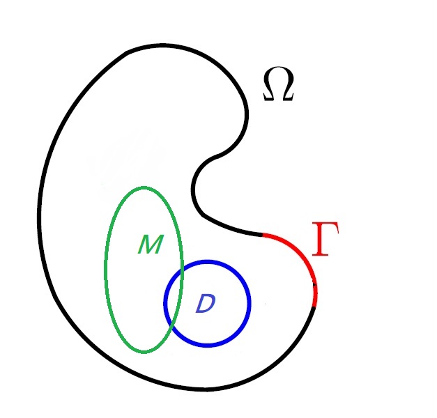
Figure 1. Schematic illustration of the field localizing and concentration.

The rest of the paper is organized as follows. In Section 2, we present results on the well-posedness of the time-harmonic anisotropic Maxwell system. We also provide the unique continuation property (UCP) for the anisotropic Maxwell system, whenever the coefficients $\mu$ and $\epsilon$ are piecewise Lipschitz continuous matrix-valued functions. In Section 3, we demonstrate that there exist localized electromagnetic fields, which proves Theorem 1.1. The method relies on functional analysis techniques. In Section 4 we prove a related Runge approximation property for the anisotropic Maxwell system with parital boundary data.

2. The anisotropic Maxwell system in a bounded domain

In this section, we summarize some useful results of the Maxwell system, including unique solvability and a unique continuation property. Throughout this section let $\Omega\subset\mathbb{R}^{3}$ be a bounded Lipschitz domain.

2.1. Spaces and traces

We introduce the spaces

$$H(\operatorname{div},\Omega) :=\left\{E\in L^{2}(\Omega)^{3};\quad\nabla\cdot E\in L^{2}(\Omega)\right\},$$

$$H(\mathrm{curl},\Omega) :=\left\{E\in L^{2}(\Omega)^{3};\quad\nabla\times E\in L^{2}(\Omega)^{3}\right\},$$

and the tangential trace operators

$$\gamma_{t}: \ H(\mathrm{curl},\Omega)\to H^{-1/2}(\mathrm{div}_{\partial\Omega},\partial\Omega),\quad E\mapsto\gamma_{t}E:=\nu\times E|_{\partial\Omega},$$

$$\gamma_{T}: \ H(\mathrm{curl},\Omega)\to H^{-1/2}(\mathrm{curl}_{\partial\Omega},\partial\Omega),\quad E\mapsto\gamma_{T}E:=\nu\times(E\times\nu)|_{\partial\Omega},$$

where here and in the following all functions are complex-valued unless indicated otherwise. Then $\gamma_{t}$ and $\gamma_{T}$ are surjective bounded linear operators with bounded right inverses $\gamma_{t}^{-1}$ and and $\gamma_{T}^{-1}$, the space $H^{-1/2}(\mathrm{div}_{\partial\Omega},\partial\Omega)$ can be identified with the dual of $H^{-1/2}(\mathrm{curl}_{\partial\Omega},\partial\Omega)$, and for all $E,F\in H(\mathrm{curl},\Omega)$ we have the integration by parts formula

$$\int_{\Omega}(\nabla\times E)\cdot F\,{\rm{d}}x-\int_{\Omega}E\cdot(\nabla\times F)\,{\rm{d}}x=\int_{\partial\Omega}\left(\nu\times E|_{\partial\Omega}\right)\cdot\left(\nu\times(F|_{\partial\Omega}\times\nu)\right)\,{\rm{d}}S$$ (2.1)

(cf. [8, 34]), where the dual pairing on $H^{-1/2}(\mathrm{div}_{\partial\Omega},\partial\Omega)\times H^{-1/2}(\mathrm{curl}_{\partial\Omega},\partial\Omega)$ is written as integral for the sake of readability.

The subspace of $H(\operatorname{curl},\Omega)$-functions with vanishing tangential trace is denoted by

$$H_{0}(\operatorname{curl},\Omega) :=\{E\in H(\operatorname{curl},\Omega):\ \nu\times E|_{\partial\Omega}=0\}.$$

$H_{0}(\operatorname{curl},\Omega)$ is a closed subspace of $H(\operatorname{curl},\Omega)$ and $C_{0}^{\infty}(\Omega)^{3}$ is dense in $H_{0}(\operatorname{curl},\Omega)$, cf. [34].

To treat partial boundary data on a relatively open subset $\Gamma\subseteq\partial\Omega$ , we also introduce the space of functions on $\Gamma$ that can be extended by zero to the trace of a $H(\mathrm{curl},\Omega)$-function

$$H(\Gamma):=\text{closure of }C^{\infty}_{c}(\Gamma)\text{ in }H^{-1/2}(\mathrm{div}_{\partial\Omega},\partial\Omega).$$ (2.2)

For all $E\in H(\mathrm{curl},\Omega)$, we identify the restricted trace $\nu\times(E\times\nu)|_{\Gamma}$ with the quotient space element

$$\nu\times(E\times\nu)|_{\partial\Omega}+H(\Gamma)^{\perp}\in H^{-1/2}(\mathrm{curl}_{\partial\Omega},\partial\Omega)/H(\Gamma)^{\perp}=H(\Gamma)^{*},$$

and thus define the restricted trace operator

$$\gamma_{T}^{(\Gamma)}:\ H(\mathrm{curl},\Omega)\to H(\Gamma)^{*},\quad E\mapsto\gamma_{T}^{(\Gamma)}E:=\nu\times(E\times\nu)|_{\Gamma}.$$

2.2. Well-posedness of the anisotropic Maxwell system

Given anisotropic coefficients $\epsilon,\mu\in L^{\infty}(\Omega,\mathbb{R}^{3\times 3})$ satisfying (1.1), $k>0$, $J,K\in L^{2}(\Omega)^{3}$ and $f\in H^{-1/2}(\mathrm{div}_{\partial\Omega},\partial\Omega)$, we consider the Maxwell system for $(E,H)\in L^{2}(\Omega)^{3}\times L^{2}(\Omega)^{3}$

$$\nabla\times E-ik\mu H =K \quad\mbox{ in }\Omega,$$ (2.3)

$$\nabla\times H+ik\epsilon E =J \quad\mbox{ in }\Omega,$$ (2.4)

$$\nu\times E|_{\partial\Omega} =f.$$ (2.5)

Note that the boundary condition (2.5) is well-defined since (2.3) implies $E\in H(\operatorname{curl},\Omega)$.

For the variational formulation of (2.3)–(2.4) we introduce the sesquilinear form

$$\mathcal{B} :\ H(\operatorname{curl},\Omega)\times H(\operatorname{curl},\Omega)\to\mathbb{C},$$

$$\mathcal{B}(E,F) :=\int_{\Omega}\left(\mu^{-1}\nabla\times E\right)\cdot\left(\nabla\times\overline{F}\right)\,{\rm{d}}x-\int_{\Omega}k^{2}\epsilon E\cdot\overline{F}\,{\rm{d}}x.$$

Then we have the following variational formulation and well-posedness result.

Theorem 2.1.

1. $(E,H)\in L^{2}(\Omega)^{3}\times L^{2}(\Omega)^{3}$ solve (2.3)–(2.4) if and only if $E\in H(\operatorname{curl},\Omega)$ solves

   $$\mathcal{B}(E,F)=\int_{\Omega}ikJ\cdot\overline{F}\,{\rm{d}}x+\int_{\Omega}\left(\mu^{-1}K\right)\cdot\left(\nabla\times\overline{F}\right)\,{\rm{d}}x\quad\text{for all $F\in H_{0}(\operatorname{curl},\Omega)$,}$$

   and $H=-\dfrac{i}{k}\mu^{-1}(\nabla\times E-K)$.

2. The set of $k>0$ for which the homogeneous system (2.3)–(2.5) with $J=0$, $K=0$, and $f=0$, possesses a non-trivial solution is discrete. We call these $k$ resonance frequencies.

3. If $k$ is not a resonance frequency, then there exists a unique solution $(E,H)\in L^{2}(\Omega)^{3}\times L^{2}(\Omega)^{3}$ of (2.3)–(2.5), and the solution depends linearly and continuously on $J,K\in L^{2}(\Omega)^{3}$ and $f\in H^{-1/2}(\mathrm{div}_{\partial\Omega},\partial\Omega)$.

The proof of Theorem 2.1 follows standard arguments. Since we did not find a reference for precisely this setting, we give a proof for the sake of completeness. For the proof we will use the following lemmas.

Lemma 2.1.

$(E,H)\in L^{2}(\Omega)^{3}\times L^{2}(\Omega)^{3}$ solve (2.3)–(2.4) if and only if $E\in H(\operatorname{curl},\Omega)$ solves

$$\mathcal{B}(E,F)=\int_{\Omega}ikJ\cdot\overline{F}\,{\rm{d}}x+\int_{\Omega}\left(\mu^{-1}K\right)\cdot\left(\nabla\times\overline{F}\right)\,{\rm{d}}x\quad\text{for all $F\in H_{0}(\operatorname{curl},\Omega)$,}$$ (2.6)

and $H=-\dfrac{i}{k}\mu^{-1}(\nabla\times E-K)$.

Proof.

Let $(E,H)\in L^{2}(\Omega)^{3}\times L^{2}(\Omega)^{3}$ solve (2.3)–(2.4). Then (2.3) implies that

$$E\in H(\operatorname{curl},\Omega)\quad\text{ and }\quad H=-\frac{i}{k}\mu^{-1}(\nabla\times E-K),$$

and combining (2.3) and (2.4) we obtain

$$\nabla\times\left(\mu^{-1}\left(\nabla\times E-K\right)\right)-k^{2}\epsilon E=ikJ,$$ (2.7)

which also shows that $\mu^{-1}\left(\nabla\times E-K\right)\in H(\mathrm{curl};\Omega)$. Using (2.7) and the integration by parts formula (2.1), it follows that for all $F\in H_{0}(\mathrm{curl};\Omega)$

$$\int_{\Omega}ikJ\cdot\overline{F}\,{\rm{d}}x =\int_{\Omega}\left(\nabla\times\left(\frac{1}{\mu}\left(\nabla\times E-K\right)\right)\right)\cdot\overline{F}\,{\rm{d}}x-\int_{\Omega}k^{2}\epsilon E\cdot\overline{F}\,{\rm{d}}x$$

$$=\int_{\Omega}\left(\mu^{-1}\left(\nabla\times E-K\right)\right)\cdot\left(\nabla\times\overline{F}\right)\,{\rm{d}}x-\int_{\Omega}k^{2}\epsilon E\cdot\overline{F}\,{\rm{d}}x,$$

and thus (2.6) holds.

On the other hand, if $E\in H(\operatorname{curl},\Omega)$ fulfills (2.6) for all $F\in H_{0}(\operatorname{curl},\Omega)$, then this also holds for all $F\in C_{0}^{\infty}(\Omega)^{3}$ which (by the definition of distributional derivatives) shows that

$$\nabla\times\left(\mu^{-1}\nabla\times E\right)-k^{2}\epsilon E=ikJ+\nabla\times\left(\mu^{-1}K\right),$$

and thus

$$\frac{1}{ik}\nabla\times\left(\mu^{-1}(\nabla\times E-K)\right)+ik\epsilon E=J.$$

Defining $H:=\dfrac{1}{ik}\mu^{-1}(\nabla\times E-K)$ it follows that $H\in H(\mathrm{curl};\Omega)$ and that $E$ and $H$ solve (2.3)–(2.4). ∎

If $H(\operatorname{curl},\Omega)$ was compactly embedded in $L^{2}(\Omega)$, then Theorem 2.1 would immediately follow from Lemma 2.1 by Fredholm theory arguments. Unfortunately this is not the case, so that we require an additional variational formulation on the space

$$\mathcal{H} :=\{E\in L^{2}(\Omega)^{3}:\ \nabla\times E\in L^{2}(\Omega)^{3},\ \nabla\cdot(\epsilon E)=0,\ \nu\times E|_{\partial\Omega}=0\},$$

which is compactly embedded in $L^{2}(\Omega)^{3}$, by using the following inequality

$$\|\nabla E\|_{L^{2}(\Omega)}\leq C\left\{\|\nabla\times E\|_{L^{2}(\Omega)}+\|\nabla\cdot(\epsilon E)\|_{L^{2}(\Omega)}+\|\nu\times E\|_{H^{1/2}(\partial\Omega)}\right\},$$

for some positive constant $C$ depending only on $\epsilon$ and $\Omega$ (for example, see [37, Theorem 2.3]). We will now first consider the Maxwell system with homogeneous boundary data and divergence free electric currents, so that the solution lies in $\mathcal{H}$. After that we will show that the general Maxwell system can always be transformed (or gauged) to fulfill this condition.

Lemma 2.2.

For $f=0$ and $\nabla\cdot J=0$, $(E,H)\in L^{2}(\Omega)^{3}\times L^{2}(\Omega)^{3}$ solves (2.3)–(2.5) if and only if $E\in\mathcal{H}$ solves

$$\mathcal{B}(E,F)=\int_{\Omega}ikJ\cdot\overline{F}\,{\rm{d}}x+\int_{\Omega}\left(\mu^{-1}K\right)\cdot\left(\nabla\times\overline{F}\right)\,{\rm{d}}x\quad\text{for all $F\in\mathcal{H}$,}$$ (2.8)

and $H=-\dfrac{i}{k}\mu^{-1}(\nabla\times E-K)$.

Proof.

If $(E,H)\in L^{2}(\Omega)^{3}\times L^{2}(\Omega)^{3}$ fulfill (2.3)–(2.5), then clearly $E\in\mathcal{H}$ and Lemma 2.1 shows that (2.8) is fulfilled for all $F\in\mathcal{H}\subset H_{0}(\operatorname{curl},\Omega)$.

To prove the other direction, let $E\in\mathcal{H}$ fulfill (2.8) for all $F\in\mathcal{H}$. Given $\Phi\in H_{0}(\operatorname{curl},\Omega)$, there exists a solution $\varphi\in H_{0}^{1}(\Omega)$ of

$$\nabla\cdot(\epsilon\nabla\varphi)=-\nabla\cdot(\epsilon\Phi)$$

and thus $F:=\Phi+\nabla\varphi\in\mathcal{H}$. Using (2.8) it follows that for

$$\mathcal{B}(E,\Phi) =\mathcal{B}(E,F)-\mathcal{B}(E,\nabla\varphi)$$

$$=\int_{\Omega}ikJ\cdot\overline{F}\,{\rm{d}}x+\int_{\Omega}\left(\mu^{-1}K\right)\cdot\left(\nabla\times\overline{F}\right)\,{\rm{d}}x+\int_{\Omega}k^{2}\epsilon E\cdot\nabla\overline{\varphi}\,{\rm{d}}x$$

$$=\int_{\Omega}ikJ\cdot\overline{\Phi}\,{\rm{d}}x+\int_{\Omega}\left(\mu^{-1}K\right)\cdot\left(\nabla\times\overline{\Phi}\right)\,{\rm{d}}x,$$

where we used $\nabla\times(\nabla\varphi)=0$, $\nabla\cdot J=0$, $\nabla\cdot(\epsilon E)=0$ and $\varphi|_{\partial\Omega}=0$. ∎

We recall that we call $k>0$ a resonance frequency, if the homogeneous Maxwell system (2.3)–(2.5) with $J=0$, $K=0$ and $f=0$ admits a non-trivial solution.

Lemma 2.3.

If $k>0$ is not a resonance frequency, then for every $J,K\in L^{2}(\Omega)^{3}$ with $\nabla\cdot J=0$ and $f=0$, there exists a unique solution $(E,H)\in L^{2}(\Omega)^{3}\times L^{2}(\Omega)^{3}$ of (2.3)–(2.5), and the solution depends continuously on $J,K\in L^{2}(\Omega)^{3}$. Moreover, the set of resonance frequencies is discrete.

Proof.

Lemma 2.2 yields that $(E,H)\in L^{2}(\Omega)\times L^{2}(\Omega)$ solves (2.3)–(2.5) if and only if

$$\left(\mathcal{A}+\mathcal{K}(k)\right)E=l,$$

where $\mathcal{A},\mathcal{K}(k):\ \mathcal{H}\to\mathcal{H}^{*}$ are defined by

$$\langle\mathcal{A}E,F\rangle:=\int_{\Omega}\left(\mu^{-1}\nabla\times E\right)\cdot\left(\nabla\times F\right)\,{\rm{d}}x+\int_{\Omega}E\cdot F\,{\rm{d}}x,\quad \text{ for all }E,F\in\mathcal{H},$$

$$\langle\mathcal{K}(k)E,F\rangle:=-\int_{\Omega}(1+k^{2}\epsilon)E\cdot F\,{\rm{d}}x,\quad \text{ for all }E,F\in\mathcal{H},$$

and $l\in\mathcal{H}^{*}$ is defined by

$$\langle l,F\rangle=\int_{\Omega}ikJ\cdot F\,{\rm{d}}x+\int_{\Omega}\left(\mu^{-1}K\right)\cdot\left(\nabla\times F\right)\,{\rm{d}}x,\quad\text{ for all }F\in\mathcal{H},$$

where $\mathcal{H}^{*}$ is the dual space of $\mathcal{H}$.

Then $\mathcal{A}$ is a coercive linear bounded operator and thus continuously invertible due to the Lax-Milgram theorem. For every $k\in\mathbb{C}$, $\mathcal{K}(k):\ \mathcal{H}\to\mathcal{H}^{*}$ is a linear compact operator due to the compact imbedding of $\mathcal{H}$ into $L^{2}(\Omega)^{3}$. $l\in\mathcal{H}^{*}$ depends linearly and continously on $J,K\in L^{2}(\Omega)^{3}$. It thus follows from the Fredholm alternative, that $\mathcal{A}+\mathcal{K}(k)$ is continuously invertible if it is injective, i.e., if $k>0$ is not a resonance frequency.

Moreover, $\mathcal{K}(k)$ depends analytically on $k$, and for $\widehat{k}:=i$, $\mathcal{A}+\mathcal{K}(\widehat{k})$ is coercive and thus continuously invertible. Hence, it follows from the analytic Fredholm theorem, that the set of resonances is discrete. ∎

Now we extend this result to non-homogeneous boundary data $f$ and non-divergence-free currents $J$ and prove theorem 2.1.

Proof of Theorem 2.1. (a) follows from Lemma 2.1. (b) and the uniqueness of the solution of the Maxwell system is proven in Lemma 2.3. To prove existence of the solution, let $J,K\in L^{2}(\Omega)^{3}$ and $f\in H^{-1/2}(\mathrm{div}_{\partial\Omega},\partial\Omega)$. We define $E_{f}=\gamma_{t}^{-1}f\in H(\operatorname{curl},\Omega)$, i.e., $\nu\times E_{f}|_{\partial\Omega}=f$ and $E_{f}$ depends continuously and linear on $f$. Moreover let $\psi\in H_{0}^{1}(\Omega)$ solve

$$\nabla\cdot(ik\epsilon\nabla\psi)=\nabla\cdot(J-ik\epsilon E_{f}),$$

which also depends continuously and linearly on $J$ and $E_{f}$.

It follows from Lemma 2.3 that there exists a solution $(E_{0},H)\in L^{2}(\Omega)^{3}\times L^{2}(\Omega)^{3}$ of the gauged system

$$\begin{cases}\nabla\times E_{0}-ik\mu H=K-\nabla\times E_{f}&\mbox{ in }\Omega,\\ \nabla\times H+ik\epsilon E_{0}=J-ik\epsilon E_{f}-ik\epsilon\nabla\psi&\mbox{ in }\Omega,\\ \nu\times E_{0}|_{\partial\Omega}=0,\end{cases}$$

and $E_{0}$ and $H$ depends linearly and continuously on $K-\nabla\times E_{f}\in L^{2}(\Omega)^{3}$ and $J-ik\epsilon E_{f}-ik\epsilon\nabla\psi\in L^{2}(\Omega)^{3}$. Hence, $E:=E_{0}+E_{f}+\nabla\psi$ and $H$ solve (2.3)–(2.5) and depend linearly and continuously on $J,K\in L^{2}(\Omega)^{3}$ and $f\in H^{-1/2}(\mathrm{div}_{\partial\Omega},\partial\Omega)$. $\Box$

2.3. Unique continuation

The unique continuation property (UCP) is an important property to study the localized fields for differential equations. The UCP for the anisotropic Maxwell system was studied by [29, 35], which can help us to construct localized electromagnetic fields.

Definition 2.1.

We say that $(\epsilon,\mu)$ satisfies the UCP in $\Omega$ if $(E,H)\in H(\mathrm{curl};\Omega)\times H(\mathrm{curl};\Omega)$ is a solution of

$$\begin{cases}\nabla\times E-ik\mu H=0&\mbox{ in }\Omega,\\ \nabla\times H+ik\epsilon E=0&\mbox{ in }\Omega,\end{cases}$$ (2.9)

which vanishes in a nonempty open set $D$ in $\Omega$, then $(E,H)\equiv(0,0)$ in $\Omega$.

Theorem 2.2 (Unique continuation property).

The following properties hold:

• Let $\epsilon,\mu\in L^{\infty}(\Omega,\mathbb{R}^{3\times 3})$ be piecewise Lipschitz continuous matrix-valued functions in $\Omega$ satisfying (1.1). Suppose that $(E,H)\in L^{2}(\Omega)^{3}\times L^{2}(\Omega)^{3}$ solves (2.9). If $(E,H)=(0,0)$ in some nonempty open subset $D\subset\Omega$, we have $(E,H)=(0,0)$ in $\Omega$.

• Let $\mathcal{F}$ be a closed set in $\Omega$ such that $\Omega\setminus\mathcal{F}$ is connected to a relatively open boundary part $\Gamma\subseteq\partial\Omega$. Let $(E,H)\in H(\mathrm{curl};\Omega)\times H(\mathrm{curl};\Omega)$ solve

  $$\begin{cases}\nabla\times E-ik\mu H=0&\mbox{ in }\Omega\backslash\mathcal{F},\\ \nabla\times H+ik\epsilon E=0&\mbox{ in }\Omega\backslash\mathcal{F}.\end{cases}$$

  If $\nu\times E|_{\Gamma}=\nu\times H|_{\Gamma}=0$ on $\Gamma$, then $(E,H)=(0,0)$ in $\Omega\backslash\mathcal{F}$.

Proof.

(a) The UCP of the Maxwell system was proved by Leis [29] when $\epsilon,\mu$ are $C^{2}$ scalar functions. When $\epsilon,\mu$ are Lipschitz continuous anisotropic parameters, the UCP was proved by Nguyen-Wang [35]. In [31], Liu, Rondi and Xiao have shown that the UCP holds for piecewise Lipschitz continuous matrix-valued functions $\epsilon$ and $\mu$ (see [31, Section 2]). We omit the proof here.

(b) Let $\mathcal{O}$ be a nonempty open set in $\mathbb{R}^{3}$ such that $\mathcal{O}\cap\partial\Omega=\Gamma$ and $\mathcal{F}\subset\mathcal{O}$. In the set $\Omega\cup\mathcal{O}$, we define

$$\widehat{\epsilon}:=\begin{cases}\epsilon&\mbox{ in }\Omega\\ 1&\mbox{ in }\mathcal{O}\backslash\Omega\end{cases}\mbox{ and }\widehat{\mu}=\begin{cases}\mu&\mbox{ in }\Omega\\ 1&\mbox{ in }\mathcal{O}\backslash\Omega\end{cases}.$$

Since $\nu\times E=\nu\times H=0$ on $\Gamma$, we can extend $(E,H)$ by $(0,0)$ and define the extension functions

$$\widehat{E}:=\begin{cases}E&\mbox{ in }\Omega\\ 0&\mbox{ in }\mathcal{O}\backslash\Omega\end{cases}\mbox{ and }\widehat{H}:=\begin{cases}H&\mbox{ in }\Omega\\ 0&\mbox{ in }\mathcal{O}\backslash\Omega\end{cases}.$$

First, we prove that $(\widehat{E},\widehat{H})\in H(\mathrm{curl};\Omega\cup\mathcal{O})\times H(\mathrm{curl};\Omega\cup\mathcal{O})$. For any $\phi\in C_{c}^{\infty}(\Omega\cup\mathcal{O})$, we have

$$\int_{\Omega\cup\mathcal{O}}\widehat{E}\cdot(\nabla\times\phi)dx = \int_{\Omega}E\cdot(\nabla\times\phi)dx$$

$$= \int_{\Omega}\left(\nabla\times E\right)\cdot\phi dx+\int_{\partial\Omega}E\cdot(\nu\times\phi)dS$$

$$= \int_{\Omega\cup\mathcal{O}}\left(\left(\nabla\times E\right)\chi_{\Omega}\right)\cdot\phi dx,$$

where we have used $E\cdot(\nu\times\phi)=-\phi\cdot\left(\nu\times E\right)=0$ on $\Gamma$ and $\phi=0$ on $\partial\Omega\backslash\Gamma$. This shows that $\widehat{E}\in H(\mathrm{curl};\Omega\cup\mathcal{O})$ and that $\nabla\times\widehat{E}$ is the zero extension of $\nabla\times E$. The same holds for $\widehat{H}$, and thus it also follows that $(\widehat{E},\widehat{H})$ is a solution of

$$\begin{cases}\nabla\times\widehat{E}-ik\widehat{\mu}\widehat{H}=0&\mbox{ in }\left(\Omega\cup\mathcal{O}\right)\backslash\mathcal{F},\\ \nabla\times\widehat{H}+ik\widehat{\epsilon}\widehat{E}=0&\mbox{ in }\left(\Omega\cup\mathcal{O}\right)\backslash\mathcal{F}.\end{cases}$$

Notice that $\widehat{\epsilon}$ and $\widehat{\mu}$ are piecewise Lipschitz continuous functions fulfilling the ellipticity condition (1.1) and recall that $\widehat{E}=\widehat{H}=0$ in $\mathcal{O}\backslash\overline{\Omega}$ (a nonempty open set). Then by using (a), the UCP gives $\widehat{E}\equiv\widehat{H}\equiv 0$ in $\left(\Omega\cup\mathcal{O}\right)\backslash\mathcal{F}$ and completes the proof. ∎

3. Localized electromagnetic fields

We will now present the main result on localizing and concentrating electromagnetic field. We show that there exists boundary data (supported on an arbitrarily small boundary part) which generates an electromagnetic field with arbitrarily high energy on one part of the considered domain and arbitrarily small energy on another part. This extends the related results in [12] for the conductivity equation and [20] for the Helmholtz equation to the more practical and challenging Maxwell system. In this section, we prove the existence of localized fields by using the functional analysis techniques from [12]. Recall our main result as follows.

Theorem 3.1.

Let $\Omega\subset\mathbb{R}^{3}$ be a bounded Lipschitz domain and $\Gamma\subseteq\partial\Omega$ be a relatively open piece of the boundary. Let $\epsilon,\mu\in L^{\infty}(\Omega,\mathbb{R}^{3\times 3})$ be real-valued, piecewise Lipschitz continuous functions satisfying (1.1) and $k\in\mathbb{R}_{+}$ be a non-resonant wavenumber. Let $D\Subset\Omega$ be a closed set with connected complement $\Omega\setminus D$. For every open set $M\subseteq\Omega$ with $M\not\subseteq D$ (see Figure 1 for the schematic illustration), there exists a sequence $\left\{f^{(\ell)}\right\}_{\ell\in\mathbb{N}}\subset C_{c}^{\infty}(\Gamma)$ such that the electromagnetic fields fulfill

$$\int_{M}\left(|E^{(\ell)}|^{2}+|H^{(\ell)}|^{2}\right)\,{\rm{d}}x\to\infty\quad\mbox{ and }\quad\int_{D}\left(|E^{(\ell)}|^{2}+|H^{(\ell)}|^{2}\right)\,{\rm{d}}x\to 0\mbox{ as }\ell\to\infty,$$ (3.1)

where, for $\ell\in\mathbb{N}$, $(E^{(\ell)},H^{(\ell)})\in L^{2}(\Omega)^{3}\times L^{2}(\Omega)^{3}$ is a solution of

$$\nabla\times E^{(\ell)}-ik\mu H^{(\ell)} =0 \quad\mbox{ in }\Omega,$$ (3.2)

$$\nabla\times H^{(\ell)}+ik\epsilon E^{(\ell)} =0 \quad\mbox{ in }\Omega,$$ (3.3)

with boundary data

$$\nu\times E^{(\ell)}|_{\partial\Omega}=\begin{cases}f^{(\ell)}&\mbox{ on }\Gamma,\\ 0&\mbox{ otherwise.}\end{cases}$$ (3.4)

Proof of Theorem 3.1. We first note that it suffices to prove the theorem for an open subset of $M$. Hence, without loss of generality, we can assume that $M\Subset\Omega$ is open, $\overline{M}\cap D=\emptyset$ and that $\Omega\setminus(\overline{M}\cup D)$ is connected. We follow the localized potentials strategy in [12, 21, 20] and first describe the energy terms in Theorem 3.1 as operator evaluations. Then we will show that the ranges of the adjoints of these operators have trivial intersection. A functional analytic relation between the norm of an operator evaluation and the range of its adjoint will then yield that the operator evaluations cannot be bounded by each other, which then shows that we can drive one energy term in theorem 3.1 to infinity and the other one to zero.

For a measurable subset $O\subseteq\Omega$, we define

$$\mathcal{L}_{O}:\ H(\Gamma)\to L^{2}(O)^{3}\times L^{2}(O)^{3}\mbox{ by }f\mapsto(E|_{O},H_{O}),$$

where $H(\Gamma)$ was defined in (2.2), and $(E,H)\in L^{2}(\Omega)^{3}\times L^{2}(\Omega)^{3}$ solve (3.2)–(3.3) with boundary data $\nu\times E|_{\partial\Omega}=f$. Now we characterize the adjoint of this operator.

Lemma 3.1.

The adjoint of $\mathcal{L}_{O}$ is given by

$$\mathcal{L}_{O}^{*}:\ L^{2}(O)^{3}\times L^{2}(O)^{3}\to H(\Gamma)^{*}\mbox{ by }(J,K)\to-\nu\times(\widetilde{H}\times\nu)|_{\Gamma},$$

where $(\widetilde{E},\widetilde{F})\in L^{2}(\Omega)^{3}\times L^{2}(\Omega)^{3}$ solve the (adjoint) Maxwell system (cf. Theorem 2.1)

$$\begin{cases}\nabla\times\widetilde{E}+ik\mu\widetilde{H}=K\chi_{O}&\mbox{ in }\Omega,\\ \nabla\times\widetilde{H}-ik\epsilon\widetilde{E}=J\chi_{O}&\mbox{ in }\Omega,\\ \nu\times\widetilde{E}|_{\partial\Omega}=0,\end{cases}$$

and $K\chi_{O}$ and $J\chi_{O}$ denote the zero extensions of $K$ and $J$ to $\Omega$.

Proof.

As in subsection 2.1, we write the dual pairing on $H(\Gamma)^{*}\times H(\Gamma)$ as an integral for the sake of readability. With this notation we have that

$$\int_{\Gamma}\overline{f}\cdot\mathcal{L}_{O}^{*}(J,K)\,{\rm{d}}s$$

$$=\int_{O}(J,K)\cdot\overline{(E|_{O},H_{O})}\,{\rm{d}}x=\int_{\Omega}J\chi_{O}\cdot\overline{E}\,{\rm{d}}x+\int_{\Omega}K\chi_{O}\cdot\overline{H}\,{\rm{d}}x$$

$$=\int_{\Omega}J\chi_{O}\cdot\overline{E}\,{\rm{d}}x-\frac{1}{ik}\int_{\Omega}K\chi_{O}\cdot\left(\mu^{-1}\nabla\times\overline{E}\right)\,{\rm{d}}x$$

$$=\int_{\Omega}\left(\nabla\times\widetilde{H}-ik\epsilon\widetilde{E}\right)\cdot\overline{E}\,{\rm{d}}x-\frac{1}{ik}\int_{\Omega}\left(\nabla\times\widetilde{E}+ik\mu\widetilde{H}\right)\cdot\left(\mu^{-1}\nabla\times\overline{E}\right)\,{\rm{d}}x$$

$$=\int_{\Omega}\left(\nabla\times\widetilde{H}\right)\cdot\overline{E}\,{\rm{d}}x-\int_{\Omega}\widetilde{H}\cdot\left(\nabla\times\overline{E}\right)\,{\rm{d}}x$$

$$\quad-\frac{1}{ik}\left(\int_{\Omega}\left(\mu^{-1}\nabla\times\overline{E}\right)\cdot\left(\nabla\times\widetilde{E}\right)\,{\rm{d}}x-\int_{\Omega}k^{2}\epsilon\overline{E}\cdot\widetilde{E}\,{\rm{d}}x\right)$$

$$=-\int_{\partial\Omega}\left(\nu\times\overline{E}|_{\partial\Omega}\right)\cdot\left(\nu\times\widetilde{H}|_{\partial\Omega}\times\nu\right)\,{\rm{d}}S=-\int_{\Gamma}\overline{f}\cdot\left(\nu\times\widetilde{H}|_{\Gamma}\times\nu\right)\,{\rm{d}}S,$$

where we used that $\epsilon$ and $\mu$ are real-valued and symmetric. We also utilized the integration by parts formula (2.1) and that $\widetilde{E}\in H_{0}(\operatorname{curl},\Omega)$ implies that

$$\int_{\Omega}\left(\mu^{-1}\nabla\times\overline{E}\right)\cdot\left(\nabla\times\widetilde{E}\right)\,{\rm{d}}x-\int_{\Omega}k^{2}\epsilon\overline{E}\cdot\widetilde{E}\,{\rm{d}}x=0$$

by Theorem 2.1 (a). ∎

Then we have the following property for the ranges of the adjoint operators $\mathcal{L}_{M}^{*}$ and $\mathcal{L}_{D}^{*}$.

Lemma 3.2.

$\mathcal{L}_{M}$ and $\mathcal{L}_{D}^{*}$ are injective, the ranges $\mathscr{R}(\mathcal{L}_{M}^{*})$ and $\mathscr{R}(\mathcal{L}_{D}^{*})$ are both dense in $H(\Gamma)^{*}$, and

$$\mathscr{R}(\mathcal{L}_{M}^{*})\cap\mathscr{R}(\mathcal{L}_{D}^{*})=\{0\}.$$ (3.5)

Proof.

The proof follows from the UCP for the Maxwell system. By Theorem 2.2 (a), one can see that $\mathcal{L}_{M}$ and $\mathcal{L}_{D}$ are injective, and therefore $\mathscr{R}(\mathcal{L}_{M\cap B}^{*})$ and $\mathscr{R}(\mathcal{L}_{D}^{*})$ both are dense in $H(\Gamma)^{*}$.

To prove (3.5), let $g\in\mathscr{R}(\mathcal{L}_{M}^{*})\cap\mathscr{R}(\mathcal{L}_{D}^{*})$, then there exist $J_{M},K_{M}\in L^{2}(M)$ and $J_{D},K_{D}\in L^{2}(D)$ such that the solutions $(E_{M},H_{M}),(E_{D},H_{D})\in L^{2}(\Omega)^{3}\times L^{2}(\Omega)^{3}$ of

$$\begin{cases}\nabla\times E_{M}+ik\mu H_{M}=K_{M}\chi_{M}&\mbox{ in }\Omega\\ \nabla\times H_{M}-ik\epsilon E_{M}=J_{M}\chi_{M}&\mbox{ in }\Omega\\ \nu\times E_{M}|_{\partial\Omega}=0&\mbox{ on }\partial\Omega\end{cases}\mbox{ and }\begin{cases}\nabla\times E_{D}+ik\mu H_{D}=K_{D}\chi_{D}&\mbox{ in }\Omega\\ \nabla\times H_{D}-ik\epsilon E_{D}=J_{D}\chi_{D}&\mbox{ in }\Omega\\ \nu\times E_{D}|_{\partial\Omega}=0&\mbox{ on }\partial\Omega\end{cases}$$

fulfill

$$\nu\times(H_{M}\times\nu)|_{\Gamma}=g=\nu\times(H_{D}\times\nu)|_{\Gamma}.$$

Since $\Omega\setminus(\overline{M}\cup D)$ is connected, we obtain by using Theorem 2.2 (b) that

$$E_{M}=E_{D}\mbox{ in }\Omega\setminus(\overline{M}\cup D).$$

Hence, we can define

$$\mathbb{E}:=\begin{cases}E_{D}&\mbox{ in }M\\ E_{M}&\mbox{ in }D\\ E_{D}=E_{M}&\mbox{ in }\Omega\setminus(\overline{M}\cup D)\end{cases},\mbox{ and }\mathbb{H}:=\begin{cases}H_{D}&\mbox{ in }M\\ H_{M}&\mbox{ in }D\\ H_{D}=H_{M}&\mbox{ in }\Omega\setminus(\overline{M}\cup D)\end{cases}.$$

As in the proof of UCP, Theorem 2.2 (b), it is easy to see that $(\mathcal{E},\mathcal{H})\in L^{2}(\Omega)^{3}\times L^{2}(\Omega)^{3}$ is a solution of

$$\begin{cases}\nabla\times\mathbb{E}+ik\mu\mathbb{H}=0&\mbox{ in }\Omega,\\ \nabla\times\mathbb{H}-ik\epsilon\mathbb{E}=0&\mbox{ in }\Omega,\\ \nu\times\mathbb{E}|_{\partial\Omega}=0&\mbox{ on }\partial\Omega.\end{cases}$$

Since $k$ is non-resonant, it follows that $(\mathbb{E},\mathbb{H})=(0,0)$ so that $g=0$. This completes the proof.∎

Now we can use the following tool from functional analysis.

Lemma 3.3.

Let $X$, $Y_{1}$ and $Y_{2}$ be Hilbert spaces, and $\mathcal{A}_{1}:\ X\to Y_{1}$ and $\mathcal{A}_{2}:\ X\to Y_{2}$ be linear bounded operators. Then

$$\exists C>0:\ \lVert\mathcal{A}_{1}x\rVert\leq C\lVert\mathcal{A}_{2}x\rVert\quad\forall x\in X\quad\text{ if and only if }\quad\mathscr{R}(\mathcal{A}_{1}^{*})\subseteq\mathscr{R}(\mathcal{A}_{2}^{*}).$$

Proof.

This is proven for reflexive Banach spaces in [12, Lemma 2.5]. ∎

Proof of Theorem 1.1.

From Lemma 3.2 it follows that $\mathscr{R}(\mathcal{L}_{M}^{*})\not\subseteq\mathscr{R}(\mathcal{L}_{D}^{*})$. Using Lemma 3.3 this shows that

$$\not\exists C>0:\ \lVert\mathcal{L}_{M}f\rVert\leq C\lVert\mathcal{L}_{D}f\rVert\quad\text{ for all }f\in H(\Gamma),$$

and by continuity of $\mathcal{L}_{M}$ and $\mathcal{L}_{D}$ and density of $C^{\infty}_{c}(\Gamma)\subset H(\Gamma)$ this is equivalent to

$$\not\exists C>0:\ \lVert\mathcal{L}_{M}f\rVert\leq C\lVert\mathcal{L}_{D}f\rVert\quad\text{ for all }f\in C^{\infty}_{c}(\Gamma).$$ (3.6)

Using (3.6) with $C:=\ell^{2}$ for all $\ell\in\mathbb{N}$ we thus obtain a sequence $\left\{\widetilde{f}^{(\ell)}\right\}_{\ell\in\mathbb{N}}\subset C^{\infty}_{c}(\Gamma)$ with

$$\lVert\mathcal{L}_{M}\widetilde{f}^{(\ell)}\rVert>\ell^{2}\lVert\mathcal{L}_{D}\widetilde{f}^{(\ell)}\rVert\quad\text{ for all }\ell\in\mathbb{N}.$$

By injectivity $\mathcal{L}_{M}\widetilde{f}^{(\ell)}\neq 0$ implies $\widetilde{f}^{(\ell)}\neq 0$ and $\mathcal{L}_{D}\widetilde{f}^{(\ell)}\neq 0$, so that we can define

$$f^{(\ell)}:=\dfrac{\widetilde{f}^{(\ell)}}{\ell\lVert\mathcal{L}_{D}\widetilde{f}^{(\ell)}\rVert}\in C^{\infty}_{c}(\Gamma)$$

and it follows that

$$\int_{M}\left(|E^{(\ell)}|^{2}+|H^{(\ell)}|^{2}\right)\,{\rm{d}}x =\lVert\mathcal{L}_{M}f^{(\ell)}\rVert^{2}>\ell^{2}\to\infty,$$

$$\int_{D}\left(|E^{(\ell)}|^{2}+|H^{(\ell)}|^{2}\right)\,{\rm{d}}x =\lVert\mathcal{L}_{D}f^{(\ell)}\rVert^{2}=\frac{1}{\ell^{2}}\to 0,$$

so that Theorem 1.1 is proven. ∎

Remark 3.1.

1. A constructive version of the existence proof for the localized fields can be obtained as in [12, Lemma 2.8].

2. With the same arguments as in [20, Section 4.1] one can also show that for all spaces $W\subseteq H(\Gamma)$ with finite codimension, one can find a sequence $\left\{f^{(\ell)}\right\}_{\ell\in\mathbb{N}}\subset W$ so that the corresponding electromagnetic fields fulfill (3.1). This might be useful for developing monotonicity-based reconstruction methods as in [20].

4. Runge approximation property for the partial data Maxwell system

In this section we derive an extension of the localization result in Theorem 1.1 which shows a Runge approximation property for the partial data Maxwell system that we consider of independent interest. We show that every solution of the Maxwell system on a subset of $\Omega$ with Lipschitz boundary and connected complement can be approximated arbitrarily well by a sequence of solutions on the whole domain $\Omega$ with partial boundary data. Since we can choose a solution that is zero on a part of $\Omega$ and non-zero on another part of $\Omega$, this also implies a-fortiori the localization result Theorem 1.1, cf. also [20] for the connection between Runge approximation properties and localized solutions.

Theorem 4.1.

Let $\Omega\subset\mathbb{R}^{3}$ be a bounded Lipschitz domain and $\Gamma\subseteq\partial\Omega$ be a relatively open piece of the boundary. Let $\epsilon,\mu\in L^{\infty}(\Omega,\mathbb{R}^{3\times 3})$ be real-valued, piecewise Lipschitz continuous functions satisfying (1.1) and $k\in\mathbb{R}_{+}$ be a non-resonant wavenumber.

Let $O\Subset\Omega$ be an open set with Lipschitz boundary and connected complement $\Omega\setminus\overline{O}$. For every solution $(e,h)\in L^{2}(O)^{3}\times L^{2}(O)^{3}$ of

$$\nabla\times e-ik\mu h =0 \quad\mbox{ in }O,$$ (4.1)

$$\nabla\times h+ik\epsilon e =0 \quad\mbox{ in }O,$$ (4.2)

there exists a sequence $\left\{f^{(\ell)}\right\}_{\ell\in\mathbb{N}}\subset C_{c}^{\infty}(\Gamma)$ such that the electromagnetic fields fulfill

$$\lVert E^{(\ell)}-e\rVert_{L^{2}(O)}\to 0\quad\text{ and }\quad\lVert H^{(\ell)}-h\rVert_{L^{2}(O)}\to 0\quad\text{as}\quad\ell\to\infty,$$

where $(E^{(\ell)},H^{(\ell)})\in L^{2}(\Omega)^{3}\times L^{2}(\Omega)^{3}$ solve (3.2)–(3.4).

Proof.

Let $(e,h)\in L^{2}(O)^{3}\times L^{2}(O)^{3}$ solve (4.1)–(4.2). With the operator $\mathcal{L}_{O}$ introduced in Section 3, we will show that

$$(e,h)\in\overline{\mathscr{R}(\mathcal{L}_{O})}=\left(\mathscr{R}(\mathcal{L}_{O})^{\perp}\right)^{\perp}=\mathscr{N}(\mathcal{L}_{O}^{*})^{\perp},$$ (4.3)

where closure and orthogonality are understood with respect to the $L^{2}(O)^{3}\times L^{2}(O)^{3}$-scalar product. This shows that the assertion holds with a sequence $\left\{f^{(\ell)}\right\}_{\ell\in\mathbb{N}}\subset H(\Gamma)$, and it follows by density that the assertion holds with a sequence $\left\{f^{(\ell)}\right\}_{\ell\in\mathbb{N}}\subset C_{c}^{\infty}(\Gamma)$.

To prove (4.3) let $(J,K)\in\mathscr{N}(\mathcal{L}_{O}^{*})\subseteq L^{2}(O)^{3}\times L^{2}(O)^{3}$. Then, by Lemma 3.1, there exist $(E,H)\in L^{2}(\Omega)^{3}\times L^{2}(\Omega)^{3}$ that solve

$$\begin{cases}\nabla\times E+ik\mu H=K\chi_{O}&\mbox{ in }\Omega,\\ \nabla\times H-ik\epsilon E=J\chi_{O}&\mbox{ in }\Omega,\\ \nu\times E|_{\partial\Omega}=0&\mbox{ on }\partial\Omega,\end{cases}$$

with $\nu\times(H\times\nu)|_{\Gamma}=\mathcal{L}_{O}^{*}(J,K)=0$. The unique continuation property in Theorem 2.2 implies that $(E,H)=(0,0)$ on $\Omega\setminus\overline{O}$ and thus

$$\nu\times E|_{\partial O}=0=\nu\times H|_{\partial O}.$$

Hence, using the integration by parts formula (2.1), it follows that

$$\int_{O}\left(e\cdot\overline{J}+h\cdot\overline{K}\right)\,{\rm{d}}x =\int_{O}e\cdot\left(\nabla\times\overline{H}+ik\epsilon\overline{E}\right)\,{\rm{d}}x+\int_{O}h\cdot\left(\nabla\times\overline{E}-ik\mu\overline{H}\right)\,{\rm{d}}x$$

$$=\int_{O}\left((\nabla\times e)\cdot\overline{H}+ik\epsilon e\cdot\overline{E}\right)\,{\rm{d}}x+\int_{O}\left(\nabla\times h\cdot\overline{E}-ik\mu h\cdot\overline{H}\right)\,{\rm{d}}x$$

$$=\int_{O}(\nabla\times e-ik\mu h)\cdot\overline{H}\,{\rm{d}}x+\int_{O}(\nabla\times h+ik\epsilon e)\cdot\overline{E}\,{\rm{d}}x=0.$$

This shows $(e,h)\perp(J,K)$ so that (4.3) holds, and thus the assertion is proven. ∎

Remark 4.1.

The Runge approximation property in Theorem 4.1 implies the localization property in Theorem 1.1 by the following argument. Let $D\Subset\Omega$ be a closed set with connected complement $\Omega\setminus D$. and $M\subseteq\Omega$ be an open set with $M\not\subseteq D$ (see again Figure 1). By shrinking $M$ and enlarging $D$, we can assume that $M$ is a open set and $D$ is a closed sets with Lipschitz boundaries, $\overline{M}\cup D\Subset\Omega$, $\overline{M}\cap D=\emptyset$ and that $\Omega\setminus(\overline{M}\cup D)$ is connected.

The unique continuation property in Theorem 2.2 implies that a solution of the Maxwell system in $\Omega$ with non-trivial boundary data cannot vanish identically on $M$. This shows that there exists a non-zero solution of the Maxwell system on $M$. We extend this solution by zero on $D$, and obtain a solution $(e,h)\in L^{2}(O)\times L^{2}(O)$ on $O:=M\cup\mathrm{int}D$ with $(e,h)|_{\mathrm{int}D}\equiv(0,0)$ and $(e,h)|_{M}\not\equiv(0,0)$. Then the Runge approximation sequence from Theorem 4.1 converges to zero on $D$ but not on $M$ and a simple scaling argument as in the proof of Theorem 1.1 in Section 3 gives a sequence of electromagnetic fields with

$$\int_{M}\left(|E^{(\ell)}|^{2}+|H^{(\ell)}|^{2}\right)\,{\rm{d}}x\to\infty\quad\mbox{ and }\quad\int_{D}\left(|E^{(\ell)}|^{2}+|H^{(\ell)}|^{2}\right)\,{\rm{d}}x\to 0\mbox{ as }\ell\to\infty,$$

and $\nu\times E^{(\ell)}\in C_{c}^{\infty}(\Gamma)$ for all $\ell\in\mathbb{N}$, which also proves Theorem 1.1.

Acknowledgments. H. Liu was supported by the FRG and startup grants from Hong Kong Baptist University, and Hong Kong RGC General Research Funds, 12302415 and 12302017.

References

- [1] Giovanni Alessandrini. Singular solutions of elliptic equations and the determination of conductivity by boundary measurements. Journal of Differential Equations, 84(2):252–272, 1990.
- [2] Habib Ammari, Giulio Ciraolo, Hyeonbae Kang, Hyundae Lee, and Graeme W Milton. Spectral theory of a Neumann–Poincaré-type operator and analysis of cloaking due to anomalous localized resonance. Archive for Rational Mechanics and Analysis, 208(2):667–692, 2013.
- [3] Kazunori Ando, Hyeonbae Kang, and Hongyu Liu. Plasmon resonance with finite frequencies: a validation of the quasi-static approximation for diametrically small inclusions. SIAM Journal on Applied Mathematics, 76(2):731–749, 2016.
- [4] L. Arnold and B. Harrach. Unique shape detection in transient eddy current problems. Inverse Problems, 29(9):095004, 2013.
- [5] Andrea Barth, Bastian Harrach, Nuutti Hyvönen, and Lauri Mustonen. Detecting stochastic inclusions in electrical impedance tomography. Inverse Problems, 33(11):115012, 2017.
- [6] Guy Bouchitté and Ben Schweizer. Cloaking of small objects by anomalous localized resonance. The Quarterly Journal of Mechanics & Applied Mathematics, 63(4):437–463, 2010.
- [7] Tommi Brander, Bastian Harrach, Manas Kar, and Mikko Salo. Monotonicity and enclosure methods for the p-Laplace equation. arXiv preprint arXiv:1703.02814, 2017.
- [8] Annalisa Buffa, Martin Costabel, and Dongwoo Sheen. On traces for H(curl,) in Lipschitz domains. Journal of Mathematical Analysis and Applications, 276(2):845–867, 2002.
- [9] Henrik Garde. Comparison of linear and non-linear monotonicity-based shape reconstruction using exact matrix characterizations. Inverse Probl. Sci. Eng., 26(1):33–50, 2018.
- [10] Henrik Garde and Stratos Staboulis. Convergence and regularization for monotonicity-based shape reconstruction in electrical impedance tomography. Numer. Math., 135(4):1221–1251, 2017.
- [11] Henrik Garde and Stratos Staboulis. The regularized monotonicity method: detecting irregular indefinite inclusions. arXiv preprint arXiv:1705.07372, 2017.
- [12] Bastian Gebauer. Localized potentials in electrical impedance tomography. Inverse Probl. Imaging, 2(2):251–269, 2008.
- [13] Roland Griesmaier and Bastian Harrach. Monotonicity in inverse medium scattering on unbounded domains. arXiv preprint arXiv:1802.06264, 2018.
- [14] Bastian Harrach. On uniqueness in diffuse optical tomography. Inverse Problems, 25(5):055010, 2009.
- [15] Bastian Harrach. Simultaneous determination of the diffusion and absorption coefficient from boundary data. Inverse Probl. Imaging, 6(4):663–679, 2012.
- [16] Bastian Harrach, Eunjung Lee, and Marcel Ullrich. Combining frequency-difference and ultrasound modulated electrical impedance tomography. Inverse Problems, 31(9):095003, 2015.
- [17] Bastian Harrach and Yi-Hsuan Lin. Monotonicity-based inversion of the fractional Schrödinger equation. arXiv preprint arXiv:1711.05641, 2017.
- [18] Bastian Harrach and Mach Nguyet Minh. Enhancing residual-based techniques with shape reconstruction features in electrical impedance tomography. Inverse Problems, 32(12):125002, 2016.
- [19] Bastian Harrach and Mach Nguyet Minh. Monotonicity-based regularization for phantom experiment data in electrical impedance tomography. In Bernd Hofmann, Antonio Leitao, and Jorge Passamani Zubelli, editors, New Trends in Parameter Identification for Mathematical Models, Trends Math., pages 107–120. Springer International, 2018.
- [20] Bastian Harrach, Valter Pohjola, and Mikko Salo. Monotonicity and local uniqueness for the Helmholtz equation. arXiv preprint arXiv:1709.08756, 2017.
- [21] Bastian Harrach and Jin Keun Seo. Exact shape-reconstruction by one-step linearization in electrical impedance tomography. SIAM Journal on Mathematical Analysis, 42(4):1505–1518, 2010.
- [22] Bastian Harrach and Marcel Ullrich. Monotonicity-based shape reconstruction in electrical impedance tomography. SIAM J. Math. Anal., 45(6):3382–3403, 2013.
- [23] Bastian Harrach and Marcel Ullrich. Resolution guarantees in electrical impedance tomography. IEEE Trans. Med. Imaging, 34:1513–1521, 2015.
- [24] Bastian Harrach and Marcel Ullrich. Local uniqueness for an inverse boundary value problem with partial data. Proc. Amer. Math. Soc., 145(3):1087–1095, 2017.
- [25] Victor Isakov. On uniqueness of recovery of a discontinuous conductivity coefficient. Communications on pure and applied mathematics, 41(7):865–877, 1988.
- [26] Robert Kohn and Michael Vogelius. Determining conductivity by boundary measurements. Communications on Pure and Applied Mathematics, 37(3):289–298, 1984.
- [27] Robert V Kohn and Michael Vogelius. Determining conductivity by boundary measurements II. Interior results. Communications on Pure and Applied Mathematics, 38(5):643–667, 1985.
- [28] Peter D Lax. A stability theorem for solutions of abstract differential equations, and its application to the study of the local behavior of solutions of elliptic equations. Communications on Pure and Applied Mathematics, 9(4):747–766, 1956.
- [29] Rolf Leis. Initial boundary value problems in mathematical physics. Teubner, Stuttgart/Willey, New York, 1986.
- [30] Hongjie Li, Jingzhi Li, and Hongyu Liu. On quasi-static cloaking due to anomalous localized resonance in . SIAM Journal on Applied Mathematics, 75(3):1245–1260, 2015.
- [31] Hongyu Liu, Luca Rondi, and Jingni Xiao. Mosco convergence for H(curl) spaces, higher integrability for Maxwell’s equations, and stability in direct and inverse EM scattering problems. arXiv preprint arXiv:1603.07555, 2016.
- [32] Antonio Maffucci, Antonio Vento, Salvatore Ventre, and Antonello Tamburrino. A novel technique for evaluating the effective permittivity of inhomogeneous interconnects based on the monotonicity property. IEEE Transactions on Components, Packaging and Manufacturing Technology, 6(9):1417–1427, 2016.
- [33] Graeme W Milton and Nicolae-Alexandru P Nicorovici. On the cloaking effects associated with anomalous localized resonance. In Proceedings of the Royal Society of London A: Mathematical, Physical and Engineering Sciences, volume 462, pages 3027–3059. The Royal Society, 2006.
- [34] Peter Monk. Finite element methods for Maxwell’s equations. Numerical Mathematics and Scientific Computation. Oxford University Press, New York, 2003.
- [35] Tu Nguyen and Jenn-Nan Wang. Quantitative uniqueness estimate for the Maxwell system with Lipschitz anisotropic media. Proceedings of the American Mathematical Society, 140(2):595–605, 2012.
- [36] Nicolae-Alexandru P Nicorovici, Graeme W Milton, Ross C McPhedran, and Lindsay C Botten. Quasistatic cloaking of two-dimensional polarizable discrete systems by anomalous resonance. Optics Express, 15(10):6314–6323, 2007.
- [37] Zhongwei Shen and Liang Song. On estimates in homogenization of elliptic equations of Maxwell’s type. Advances in Mathematics, 252:7–21, 2014.
- [38] Zhiyi Su, Lalita Udpa, Gaspare Giovinco, Salvatore Ventre, and Antonello Tamburrino. Monotonicity principle in pulsed eddy current testing and its application to defect sizing. In Applied Computational Electromagnetics Society Symposium-Italy (ACES), 2017 International, pages 1–2. IEEE, 2017.
- [39] A Tamburrino and G Rubinacci. A new non-iterative inversion method for electrical resistance tomography. Inverse Problems, 18(6):1809, 2002.
- [40] Antonello Tamburrino, Zhiyi Sua, Salvatore Ventre, Lalita Udpa, and Satish S Udpa. Monotonicity based imaging method in time domain eddy current testing. Electromagnetic Nondestructive Evaluation (XIX), 41:1, 2016.
- [41] Salvatore Ventre, Antonio Maffucci, François Caire, Nechtan Le Lostec, Antea Perrotta, Guglielmo Rubinacci, Bernard Sartre, Antonio Vento, and Antonello Tamburrino. Design of a real-time eddy current tomography system. IEEE Transactions on Magnetics, 53(3):1–8, 2017.
- [42] Wikipedia. Inductive charging. https://en.wikipedia.org/wiki/Inductivecharging.
- [43] Wikipedia. Telecommunication. https://en.wikipedia.org/wiki/Telecommunication.
- [44] Liangdong Zhou, Bastian Harrach, and Jin Keun Seo. Monotonicity-based electrical impedance tomography for lung imaging. Inverse Problems, accepted for publication.