Study of the $s-\bar{s}$ asymmetry in the proton

Abstract

The study of $s-\bar{s}$ asymmetry is essential to better understand of the structure of nucleon and also the perturbative and nonperturbative mechanisms for sea quark generation. Actually, the nature and dynamical origins of this asymmetry have always been an interesting subject to research both experimentally and theoretically. One of the most powerful models can lead to $s-\bar{s}$ asymmetry is the meson-baryon model (MBM). In this work, using a simplified configuration of this model suggested by Pumplin, we calculate the $s-\bar{s}$ asymmetry for different values of cutoff parameter $\Lambda$, to study the dependence of model to this parameter and also to estimate the theoretical uncertainty imposed on the results due to its uncertainty. Then, we study the evolution of distributions obtained both at next-to-leading order (NLO) and next-to-next-to-leading order (NNLO) using different evolution schemes. It is shown that the evolution of the intrinsic quark distributions from a low initial scale, as suggested by Chang and Pang, is not a good choice at NNLO using variable flavor number scheme (VFNS).

1 Introduction

It is well known now that the factorisation theorem of Quantum Chromodynamics (QCD) [1, 2] can provide a powerful tool for calculating cross sections of high energy processes, by dividing them to perturbative and nonperturbative parts. In this respect, the nonperturbative objects such as the parton distribution functions (PDFs) [3, 4, 5, 6, 7, 8, 9, 10, 11, 12, 13], polarized PDFs [14, 15, 16, 17, 18, 19, 20], nuclear PDFs [21, 22, 23, 24, 25], and fragmentation functions (FFs) [26, 27, 28, 29] play an essential role for testing QCD, describing the experimental data, and searching New Physics. Among them, the PDFs have always been of particular importance. Actually, more accurate PDFs are very essential for theory predictions and then for better understanding of the perturbative mechanism of QCD and the structure of the nucleon. Although, recent developments in theory calculations and experimental measurements have improved our knowledge of PDFs to a large extent, the situation is not very satisfying for the case of flavor and quark-antiquark asymmetries.

It is proven that the perturbative regime of QCD can lead to the $s-\bar{s}$ asymmetry in the proton sea through the QCD evolution at next-to-next-to-leading order (NNLO) or at three loops [30]. However, it is significant only in regions of small momentum fraction $x$ and also inconsiderable in magnitude, so that cannot describe the present experimental evidences for the $s-\bar{s}$ asymmetry. In this way, the nature and dynamical origins of $s-\bar{s}$ asymmetry (as well as the $\bar{d}-\bar{u}$ flavor asymmetry [31]) have always been an interesting subject to research both experimentally and theoretically (for a review see Refs. [32, 33, 34] and references therein). It is believed now that the $s-\bar{s}$ asymmetry in the proton must has a nonperturbative origin. In this view, there are two kinds of sea quarks in the proton: “extrinsic” and “intrinsic” sea quarks which have major differences with each other. The first ones are produced perturbatively through the splitting of the gluons into $q\bar{q}$ pairs and are dominant at small $x$ regions, while the later ones are produced through the nonperturbative fluctuations of the nucleon state to five-quark states or meson plus baryon states and are dominant at large $x$ regions. In recent years, the intrinsic quarks have been a subject of study by many investigators [31, 34, 35, 36, 37, 38, 39, 40, 41, 42, 43, 44, 45].

Although the existence of the intrinsic quarks in the proton sea, for the first time, was suggested in the study of charm quark component by Brodsky, Hoyer, Peterson, and Sakai (BHPS) [46], the possible manifestations of nonperturbative effects for the $s-\bar{s}$ asymmetry was first discussed by Signal and Thomas [47], applying the meson cloud model (MCM). Moreover, Brodsky and Ma [48] proposed a light-cone baryon-meson fluctuation model to calculate the $s-\bar{s}$ asymmetry in the proton and found a significantly different result in analogy to the result of MCM. In recent years, these original ideas have been followed in many papers [49, 50, 51, 52, 53, 54, 55, 56] to shed further light on the $s-\bar{s}$ asymmetry in view of the MCM and light-cone baryon-meson fluctuation model. Another way to calculate the $s-\bar{s}$ asymmetry in the nucleon is using the chiral quark model (CQM) [57, 58]. Actually, this model has been many successes so far both for describing the flavor asymmetry and quark-antiquark asymmetry in the nucleon [60, 61, 62, 63, 64, 65, 66, 67, 68, 69, 70, 71]. In addition to these models, there is also a model called the scalar five-quark model suggested by Pumplin [59] which can give us the intrinsic components of the quark sea. It is worth noting in this context that the BHPS and scalar five-quark models cannot give us any asymmetry between the quark and antiquark distributions in the nucleon, while the MCM, CQM and light-cone baryon-meson fluctuation model can lead to this asymmetry.

Experimentally, the measurements of charm production with dimuon events in the final state in deep inelastic scattering (DIS) [72, 73, 74, 75, 76, 77], and also $W$ boson production in association with a single charm quark in proton-proton collisions [78, 79] can give us valuable information about the $s-\bar{s}$ asymmetry in the proton. It is believed that the anomaly seen by the NuTeV experiment [80] in the extraction of the Weinberg angle from neutrino-nucleus DIS can be explained by assuming the $s-\bar{s}$ asymmetry in the proton sea. For example, in Refs. [53] and [67], some first proposals to relate the $s-\bar{s}$ asymmetry to the NuTeV anomaly with phenomenological success have been presented according to the light-cone baryon-meson fluctuation model and CQM, respectively (for a review, see Ref. [81]). In addition, there have been further phenomenological applications of the $s-\bar{s}$ to some experimental facts [82, 83, 84]. For example, in Ref. [84], the authors have indicated that the difference between $\Lambda$ and $\bar{\Lambda}$ production is related to the asymmetric strange-antistrange distribution inside the nucleon.

Although the lowest moment of the $s-\bar{s}$ asymmetry, $\langle s-\bar{s}\rangle=\int_{0}^{1}[s(x)-\bar{s}(x)]dx$, is equal to zero because there is no net valence strange quark in the nucleon, the second moment of this asymmetry, $S^{-}\equiv\langle x(s-\bar{s})\rangle=\int_{0}^{1}dx\leavevmode\nobreak\ x[s(x)-\bar{s}(x)]$, can have a non-zero value. Actually, there is great interest to determine $S^{-}$ both experimentally and theoretically. For example, we can refer to the next-to-leading order (NLO) analysis of dimuon events from neutrino (antineutrino) DIS with the nucleon performed by the NuTeV Collaboration [75] which leaded to $S^{-}=0.00196\pm 0.00046\pm 0.00045$ at momentum transverse squared $Q^{2}=16$ GeV² and also the analysis performed by Barone et al. [85] using a wide range of related experimental data which leaded to $S^{-}=0.0020\pm 0.0005$ at $Q^{2}=20$ GeV². Moreover, in the first global analysis including the CCFR and NuTeV dimuon data [86], the authors found $-0.001<S^{-}<0.004$ [87]. However, it should be noted that a value of $S^{-}=0.0\pm 0.002$ has been obtained by Bentz et al. [88] at same scale that is consistent with no $s-\bar{s}$ asymmetry. As an example of theoretical estimation of $S^{-}$, one can refer to Ref. [56] where the authors achieved various values for $S^{-}$ from 0.00047 to 0.00157.

As mentioned, one of the most powerful intrinsic quark models can lead to both flavor and quark-antiquark asymmetries in the nucleon is the meson-baryon model (MBM). In the MBM framework, the nucleon sometimes fluctuates to a virtual baryon plus a meson state ($N\longrightarrow MB$). Contributions to the strange sea can come, for example, from fluctuations to the two-body state $K^{+}\Lambda^{0}$, where $K^{+}$ is a $u\bar{s}$ meson and $\Lambda^{0}$ is a $uds$ baryon. Although the MBM formalism is rather complicated computationally, Pumplin [59] has introduced a more simple configuration based on original concepts of this model and used it, for the first time, for calculating the intrinsic charm in the nucleon. A similar study has also been performed in the case of intrinsic strange [34]. It is worth noting here that in Pumplin model, the quantity plays an important role is the cutoff parameter $\Lambda$ so that its chosen value can change the final results. To be more precise, we can consider a theoretical uncertainty on the obtained distributions due to the $\Lambda$ variations. Another important issue in this respect, is the evolution of the intrinsic quark distributions using the DGLAP equations [89]. It is shown that using the non-singlet evolution equations, one can determine the intrinsic quark distributions at higher values of $Q^{2}$ [39]. In Refs [35, 36, 37], Chang and Pang were also suggested that the evolution of the intrinsic quark distributions from a very lower initial scale such as $\mu_{0}=0.3$ or 0.5 GeV leads to a better fit to the experimental data. In this work, focusing on the $s-\bar{s}$ asymmetry in the proton, we are going to investigate with more precision about two issues: 1) the dependence of the Pumplin model to the cutoff parameter $\Lambda$ and the amount of the theoretical uncertainty imposed on the results due to its variation, and 2) the evolution of $x(s-\bar{s})$ distribution and the validity of the Chang and Pang suggestion for different evolution schemes and also the order of evolution.

The paper is organised as follows. In Sec. 2, we review briefly the original MBM formalism and also the simplified configuration of it suggested by Pumplin, and present the procedure for calculating the $s-\bar{s}$ asymmetry in the proton. In Sec. 3, we calculate this asymmetry using different values of cutoff parameter $\Lambda$ to study the dependence of the model to this parameter and also to estimate the theoretical uncertainty caused by it. The study of the evolution of $s-\bar{s}$ asymmetry and then its behaviour at higher $Q^{2}$ is performed in Sec. 4. We evolve the distributions obtained both at NLO and NNLO approximation using fixed flavor number scheme (FFNS) and variable flavor number scheme (VFNS). Finally, we summarize our results and conclusions in Sec. 5.

2 Meson-baryon model framework

As mentioned in the Introduction, the possible intrinsic contribution to the $s-\bar{s}$ asymmetry was pointed out for the first time by Signal and Thomas [47] applying the MCM. The first calculation of the $s-\bar{s}$ asymmetry according the light-cone baryon-meson fluctuation model was performed by Brodsky and Ma [48]. These original works were followed in other papers [49, 50, 51, 52, 53, 54, 55, 56] in order to further investigation in this subject. Note, such asymmetry that is a natural consequence of SU(3) symmetry breaking in QCD, can also be achieved for the case of charm quark [90, 91, 92]. The main virtue of the meson-baryon model compared with the BHPS and scalar five-quark models is that it can lead to the $s-\bar{s}$ asymmetry in the nucleon sea. To be more precise, there are two origins cause this asymmetry: First is the difference between the probability distributions of the meson and baryon in the proton, and second is the difference between the strange and antistrange distributions in the baryon and meson, respectively.

According to the MBM formalism, we can consider that the wave function of the nucleon is a series involving bare nucleon and meson-baryon states so that we can write it as [49]

$$|N\rangle_{physical} =\sqrt{Z}|N\rangle_{bare}+\sum_{MB}\sum_{\lambda\lambda^{\prime}}\int dy\leavevmode\nobreak\ d^{2}\mathbf{k}_{\perp}\phi_{MB}^{\lambda\lambda^{\prime}}(y,k^{2}_{\perp})$$

$$\times|M^{\lambda}(y,\mathbf{k}_{\perp});B^{\lambda^{\prime}}(1-y,-\mathbf{k}_{\perp})\rangle.$$ (1)

In the above formula, the first term is related to the “bare” nucleon and $Z$ is the wave function renormalization constant. Moreover, the probability amplitude of the Fock state containing a virtual meson $M$ with longitudinal momentum fraction $y$, transverse momentum $\mathbf{k}_{\perp}$, and helicity $\lambda$, and a virtual baryon $B$ with longitudinal momentum fraction $1-y$, transverse momentum $-\mathbf{k}_{\perp}$, and helicity $\lambda^{\prime}$ denoted by $\phi_{MB}^{\lambda\lambda^{\prime}}(y,k^{2}_{\perp})$. Since there are no interactions among the $q$ and $\bar{q}$ in the meson-baryon components during the interaction with the hard photon in the deep inelastic process, the contributions to the quark and antiquark distributions of the nucleon can be expressed as a convolution between the distribution functions of quarks or antiquarks in the hyperon or meson with the fluctuation functions of these hadrons. In the case of strange quark, for spin dependence distributions we have [52]

$$s^{N}(x)=\sum_{BM}\,\int_{x}^{1}\frac{d\bar{y}}{\bar{y}}\,f_{BM}(\bar{y})\,s_{B}\Big{(}\frac{x}{\bar{y}}\Big{)}$$ (2)

$$\bar{s}^{N}(x)=\sum_{MB}\,\int_{x}^{1}\frac{dy}{y}\,f_{MB}(y)\,\bar{s}_{M}\Big{(}\frac{x}{y}\Big{)}$$ (3)

where ${\bar{y}}\equiv 1-y$. The fluctuation function $f_{BM}(\bar{y})$ describes the probability of a nucleon $N$ fluctuating into a baryon $B$ with longitudinal momentum fraction $\bar{y}$, while $f_{MB}(y)$ is related to the nucleon’s fluctuation into a meson $M$ with longitudinal momentum fraction $y$. Meanwhile, the $s_{B}$ and $\bar{s}_{M}$ are the strange and antistrange distributions in the baryon and meson, respectively. According to the MBM, the fluctuation functions are related to the amplitudes $\phi_{MB}^{\lambda\lambda^{\prime}}$ as follows

$$f_{MB}(y)=\sum_{\lambda\lambda^{\prime}}\int_{0}^{\infty}\,d\mathbf{k}^{2}_{\perp}|\phi_{MB}^{\lambda\lambda^{\prime}}(y,k^{2}_{\perp})|^{2}.$$ (4)

Note that we must also have the relation $f_{BM}(\bar{y})=f_{MB}(y)$ to guarantee the conservation of momentum and charge. Using the effective meson-nucleon Lagrangians, we can drive the meson-baryon probability amplitude $\phi_{MB}^{\lambda\lambda^{\prime}}$ as a function of the nucleon, baryon and meson masses, the invariant mass squared of the meson-baryon Fock state and also the vertex functions which contain the spin dependence of the amplitude [49]. As it stands, the MBM formalism is rather complicated computationally.

Beside the above presented configuration for MBM, Pumplin [59] has introduced another configuration based on original concepts of this model that is simpler computationally. According to the Pumplin model, we can use an overall relation to model both the meson-baryon probability distribution in the nucleon (equivalent to the fluctuation function) and the constituent quark distributions in the baryon or meson. To be more precise, the light-cone probability distributions can be derived directly from Feynman diagram rules and written as [59]

$$dP =\frac{g^{2}}{(16\pi^{2})^{N-1}(N-2)!}\,\prod_{j=1}^{N}dx_{j}\,\delta\left(1-\sum_{j=1}^{N}x_{j}\right)$$

$$\quad\times\int_{s_{0}}^{\infty}ds\,\frac{(s-s_{0})^{N-2}}{(s-m_{0}^{2})^{2}}\,|F(s)|^{2},$$ (5)

where

$$s_{0}=\sum_{j=1}^{N}\frac{m_{j}^{2}}{x_{j}}\,,$$ (6)

and $N$ is the number of particles with masses $m_{1},m_{2},...,m_{N}$ and spin $0$ which are coupled to a point scalar particle with mass $m_{0}$ and spin $0$ by a point-coupling $ig$. In Eq. 5, the form factor $F^{2}$ is a function of $s$ and has been included to consider further suppression of high-mass states and characterize the dynamics of the bound state. Two exponential and power-law forms have been suggested for $F^{2}$ as follows:

$$|F^{2}(s)|=\exp[-(s-m_{0}^{2})/\Lambda^{2}],$$ (7)

$$|F^{2}(s)|=(s+\Lambda^{2})^{-n}.$$ (8)

The cutoff parameter $\Lambda$ can take any value between 2 and 10 GeV.

Now, as suggested by Pumplin, having both the meson-baryon Fock state probability distribution in the nucleon and the constituent quark distributions in the baryon or meson, we can use the following relation defined as convolutions of the distributions to calculate the intrinsic quark and antiquark distributions in the nucleon,

$${{dP}\over{dx}} =\int_{0}^{1}\!dx_{1}\,f_{1}(x_{1})\int_{0}^{1}\!dx_{2}\,f_{2}(x_{2})\,\delta(x-x_{1}x_{2})$$

$$=\int_{x}^{1}{{dy}\over{y}}\,f_{1}(y)\,f_{2}(x/y).$$ (9)

For the case of intrinsic strange, we can consider six fluctuations as follows:

$$p \longrightarrow K^{+}(u\bar{s})\Lambda^{0}(uds),$$

$$p \longrightarrow K^{0}(d\bar{s})\Sigma^{+}(uus),$$

$$p \longrightarrow K^{+}(u\bar{s})\Sigma^{0}(uds),$$

$$p \longrightarrow K^{*+}(u\bar{s})\Lambda^{0}(uds),$$

$$p \longrightarrow K^{*0}(d\bar{s})\Sigma^{+}(uus),$$

$$p \longrightarrow K^{*+}(u\bar{s})\Sigma^{0}(uds).$$ (10)

However, due to high equality of the $K^{0}$ and $K^{+}$, $K^{*0}$ and $K^{*+}$, and also $\Lambda$ and $\Sigma$ physical masses, only two states $K^{+}\Lambda^{0}$ and $K^{*+}\Lambda^{0}$ lead to the different shapes for $s$ and $\bar{s}$ distributions in the nucleon and thus the $s-\bar{s}$ asymmetry [34]. As can be seen, since the involved physical masses of hadrons are determined with high accuracy from the experimental informations, the main parameter that its value can change the final results in this simplified configuration of the meson-baryon model is the cutoff parameter $\Lambda$. Actually, by calculating the distributions with different values of $\Lambda$, we can estimate the theoretical uncertainty imposed on the results due to the $\Lambda$ variation. In the next section, we present the numerical results for the $s-\bar{s}$ asymmetry in the proton and study in details the dependence of the model to cutoff parameter $\Lambda$.

3 The $s-\bar{s}$ asymmetry in the proton

The accurate determination of PDFs in the nucleon has always been an important subject in high energy physics. Since the PDFs are the nonperturbative objects, they have to be constrained in a global analysis to experimental data [3, 4, 5, 6, 7, 8, 9, 10, 11, 12, 13]. In this vein, the determination of the gluon distribution both in the nucleon [93] and nuclei [94], and also the sea quark distributions and possible asymmetries between them is of particular importance. Nowadays, thanks to many experiments provide a wide range of accurate data including the DIS, $pp$ and $p\bar{p}$ collider measurements, our knowledge of the valence quarks, and to a large extent, sea quarks and gluon distributions is satisfying. However, it is not enough in the case of flavor and quark-antiquark asymmetries.

After the observation of the Gottfried sum rule violation by the New Muon Collaboration (NMC) in measuring the proton and deuteron $F_{2}$ structure functions [95] from deep inelastic muon scattering on hydrogen and deuterium targets, it is believed that the $\bar{u}$ and $\bar{d}$ distributions in the nucleon are surely different. The antiquark flavor asymmetry $\bar{d}-\bar{u}$ was then confirmed by the HERMES Collaboration [96] in a semi-inclusive DIS (SIDIS) experiment and the FNAL E866/NuSea Collaboration [97] by measuring $pp$ and $pd$ Drell-Yan processes. All measurements demonstrated that there is a $\bar{d}$ excess over $\bar{u}$ in the nucleon sea.

Although there are some relatively clear evidences for the $s-\bar{s}$ asymmetry of the nucleon sea [75, 80, 85], in the contrary, some analyses are consistent with the strange-antistrange symmetry [88, 98]. Since these results prevent a definitive conclusion on the existence of $s-\bar{s}$ asymmetry in the nucleon, various groups choose different approaches to deal with this asymmetry in the global analysis of PDFs. For example, the NNPDF3.0 [5], MMHT14 [6] and JR14 [7] have considered $s-\bar{s}$ asymmetry in their works while the ABM12 [3], CT14 [8] and CJ15 [4] have assumed $s(x)=\bar{s}(x)$. A comparison of the results obtained for the $x(s(x)-\bar{s}(x))$ distribution and its uncertainty from the NNLO analyses of NNPDF3.0, MMHT14 and JR14 at scale $Q^{2}=4$ GeV² have been shown in Fig. 1 by the blue, red and green shaded band, respectively. As can be seen, the results have major differences can be related to the differences in used phenomenological approaches. For example, the $x(s(x)-\bar{s}(x))$ distribution from the NNPDF3.0, unlike two other PDF sets, has magnitude even at larger $x$. Furthermore, the NNPDF3.0 uncertainty is comparatively large at smaller $x$.

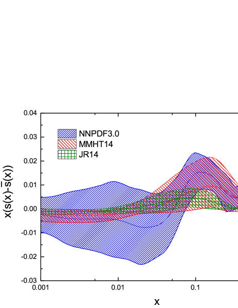
Figure 1: The NNLO $x(s(x)-\bar{s}(x))$ distribution and its uncertainty from NNPDF3.0 [5] (blue band), MMHT14 [6] (red band) and JR14 [7] (green band) PDF sets at scale $Q^{2}=4$ GeV². Results adopted from Ref. [99].

As mentioned in the Introduction, beside the phenomenologically determination of the $s-\bar{s}$ asymmetry, it can be calculated directly using some theoretical models based on the light-cone framework. In the previous section, we introduced the MBM formalism and also Pumplin model for calculating the intrinsic quark and antiquark distributions in the nucleon and the asymmetry between them. In this section, we present the numerical results for the case of strange quark and study in details the dependence of the model to cutoff parameter $\Lambda$. Its variation can be recognized as a source for generating the theoretical uncertainty imposed on the results. In this respect, we first calculate the $x(s(x)-\bar{s}(x))$ distributions related to the $K^{+}\Lambda^{0}$ and $K^{*+}\Lambda^{0}$ states separately and then sum their results to obtain the total distributions.

For the case of $K^{+}\Lambda^{0}$ state, we calculate its probability distribution in the proton using Eq. (5) with $N=2$ and $F^{2}\varpropto(s_{K\Lambda}+\Lambda^{2}_{p})^{-2}$. The same calculation is preformed using $F^{2}\varpropto(s_{u\bar{s}}+\Lambda^{2}_{K})^{-2}$ to model the $u\bar{s}$ distribution in $K^{+}$. For modeling the $uds$ distribution in $\Lambda^{0}$ we use Eq. (5) with $N=3$ and $F^{2}\varpropto(s_{uds}+\Lambda^{2}_{\Lambda})^{-2}$. Since the quarks do not exist as free particles, their masses cannot be measured directly and then they are arbitrary parameters in QCD [100]. In this work, for up and down quark masses we choose $m_{u}=m_{d}=m_{p}/3$ where $m_{p}$ is the mass of proton, while for the strange quark we should consider a larger value, for example, $m_{s}=m_{\bar{s}}=0.5$ GeV. The physical messes of the proton, $K^{+}$ meson and $\Lambda^{0}$ baryon are taken to be equal to 0.938, 0.4937 and 1.1157 in GeV, respectively. In this way, the only quantities remain are the cutoff parameters $\Lambda$. In Ref. [59], it has been suggested that we can choose any value between 2 and 10 for $\Lambda_{p}$ and between 1 and 4 for $\Lambda_{K}$ or $\Lambda_{\Lambda}$. This can effect both the shape and magnitude of the final results. Therefore, we have an uncertainty for the obtained distributions due to the $\Lambda$ uncertainty. Since it is interesting to study the dependence of the model to cutoff parameter $\Lambda$ and also to estimate the theoretical uncertainty imposed on the results, we calculate distributions for $\Lambda_{p}=2,4,10$ GeV and $\Lambda_{K}=\Lambda_{\Lambda}=1,2,4$ GeV. After the calculation of the $K^{+}\Lambda^{0}$ probability distribution in the proton, $s$ distribution in $\Lambda^{0}$ and $\bar{s}$ distribution in $K^{+}$, we can calculate the corresponding $s$ and $\bar{s}$ distributions in the proton by doing the convolution of Eq. (9) and then the asymmetry between them. As a last point, note that we normalize all distributions to 100% probability so that the quark number condition $\int_{0}^{1}dxf(x)=1$ is satisfied where $f$ is the $s$ or $\bar{s}$ distribution in related baryon or meson, respectively.

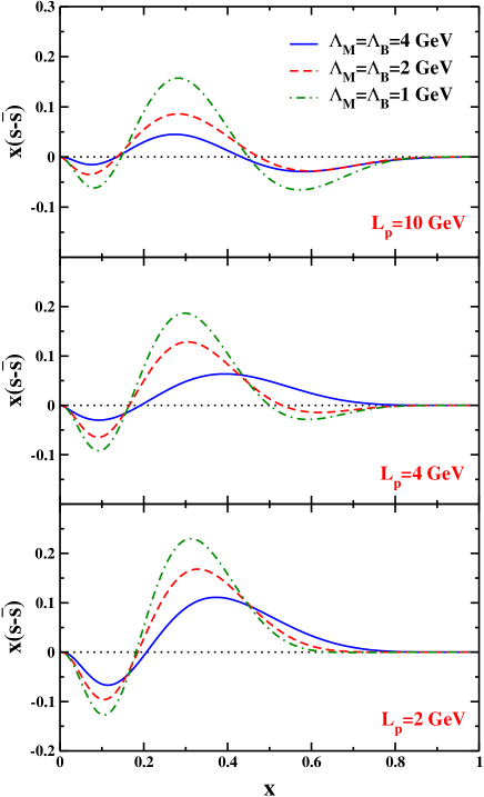
Figure 2: The $x(s(x)-\bar{s}(x))$ distributions as a function of $x$ obtained using the Pumplin model for $K^{+}\Lambda^{0}$ state with $\Lambda_{p}=10$ (top panel), 4 (middle panel) and 2 (bottom panel). In each panel, the blue solid, red dashed and green dotted-dashed curves are corresponding to the distributions for $\Lambda_{K}=\Lambda_{\Lambda}=4$, 2 and 1, respectively.

Fig. 2 shows the results obtained for $x(s(x)-\bar{s}(x))$ distributions as a function of momentum fraction $x$ for $K^{+}\Lambda^{0}$ state. The top, middle and bottom panels are related to results for $\Lambda_{p}=10$, 4 and 2 GeV, respectively. In each panel, the blue solid, red dashed and green dotted-dashed curves are corresponding to the distributions for $\Lambda_{K}=\Lambda_{\Lambda}=4$, 2 and 1 GeV, respectively. As can be seen from the top panel of Fig. 2, for $\Lambda_{p}=10$ there are two negative areas in $x(s(x)-\bar{s}(x))$ distributions, one in smaller $x$ and the other in larger $x$, and at medium $x$ the asymmetry is clearly positive. Comparing the three panels, one can see that as $\Lambda_{p}$ decreases, the negative area at larger $x$ disappears and also the magnitude of the distributions increases. Another conclusion one can draw from this figure is that for a fixed value of $\Lambda_{p}$, the magnitude of the distributions is decreased when the value of $\Lambda_{K}=\Lambda_{\Lambda}$ increases. In overall, we can conclude that the $x(s(x)-\bar{s}(x))$ distribution resulted from $K^{+}\Lambda^{0}$ state, both in shape and magnitude is very sensitive to the value of cutoff parameter $\Lambda$.

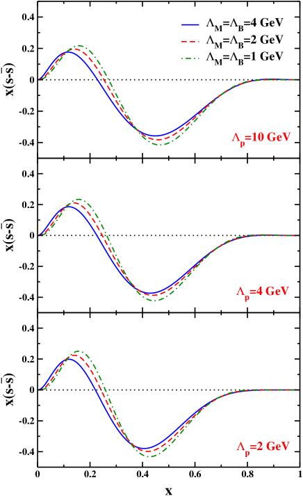
Figure 3: Same as Fig. 2 but for $K^{*+}\Lambda^{0}$ state.

As mentioned in the previous section, another meson-baryon state can lead to different shape for $s$ and $\bar{s}$ distributions in the nucleon and thus the $s-\bar{s}$ asymmetry is the $K^{*+}\Lambda^{0}$ state. The calculation procedure for this case is as before, but it should be noted that in order to avoid mass singularity we consider an effective mass $m_{\bar{s}}=0.7$ GeV for the antistrange in $K^{*+}$ as suggested in Ref. [34]. In fact, with this choice, the relation $m_{\bar{s}}+m_{u}>m_{K^{*}}$ is satisfied. Fig. 3 shows same results as Fig. 2 but for $K^{*+}\Lambda^{0}$ state. As can be seen, in this case, there are two overall regions in $x(s(x)-\bar{s}(x))$ distributions for all three values of $\Lambda_{p}$: a positive region in smaller $x$ and a negative one in medium and larger $x$. As before, when $\Lambda_{p}$ decreases, the magnitude of the distributions increases but the changes are not too drastic. By focusing on each panel separately, we find that as $\Lambda_{K}=\Lambda_{\Lambda}$ increases, the magnitude of the distribution somewhat decreases and also it shifts slightly toward smaller $x$. In overall, we can say that the $s-\bar{s}$ asymmetry resulted from $K^{*+}\Lambda^{0}$ state in not very sensitive to the value of cutoff parameter $\Lambda$.

Now we can sum the results of $x(s(x)-\bar{s}(x))$ distributions for $K^{+}\Lambda^{0}$ and $K^{*+}\Lambda^{0}$ states presented in Figs. 2 and 3 to get the total results of the $s-\bar{s}$ asymmetry in the proton. The related results have been shown in Fig. 4. As one can see, just similar to the results of $K^{*+}\Lambda^{0}$ state, there is a positive and a negative region at smaller and larger $x$ in $x(s(x)-\bar{s}(x))$ distributions for all three values of $\Lambda_{p}$. However, there is an interesting finding in the total results which is in contrary with the results for $K^{+}\Lambda^{0}$ and $K^{*+}\Lambda^{0}$ states. To be more precise, unlike before, the total distributions decrease in magnitude as $\Lambda_{p}$ decreases. Nevertheless, for a fixed value of $\Lambda_{p}$, as $\Lambda_{K}=\Lambda_{\Lambda}$ increases, the magnitude of the distribution somewhat decreases and also it shifts slightly toward smaller $x$ just like to the case of $K^{*+}\Lambda^{0}$. As a last point, note that the behavior of theoretical result obtained using the MBM is compatible with the phenomenological results of Fig. 1, only if we consider the result of $K^{+}\Lambda^{0}$ state.

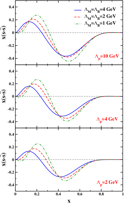
Figure 4: The total $x(s(x)-\bar{s}(x))$ distributions in the proton from the Pumplin model as a function of $x$ obtained by summing the results related to $K^{+}\Lambda^{0}$ and $K^{*+}\Lambda^{0}$ states with $\Lambda_{p}=10$ (top panel), 4 (middle panel) and 2 (bottom panel). In each panel, the blue solid, red dashed and green dotted-dashed curves are corresponding to the distributions for $\Lambda_{K}=\Lambda_{\Lambda}=4$, 2 and 1, respectively.

We can discuss now about the theoretical uncertainty of the $s-\bar{s}$ asymmetry in the proton due to the uncertainties of the cutoff parameters $\Lambda$. For this purpose, in Fig. 5, we have plotted simultaneously all distributions presented in three panels of Fig. 4 corresponding to different values of cutoff parameters $\Lambda$. In this way, we can have an estimation of theoretical uncertainty in the $s-\bar{s}$ asymmetry. Note that the description of the curves is same as before. As a result, we can conclude that the theoretical uncertainty of the $s-\bar{s}$ asymmetry due to the variation of cutoff parameters $\Lambda$ is comparatively large in all regions of momentum fraction $x$. However, for making an exact comparison between the results obtained in this section and phenomenological results for $s-\bar{s}$ asymmetry, we can consider the distribution related to $\Lambda_{K}=\Lambda_{\Lambda}=2$ GeV and $\Lambda_{p}=4$ GeV as a central distribution and calculate an error band for it due to $\Lambda$ variations. The result has been shown in Fig. 6 (red solid curve with yellow band) and compared to the NNPDF3.0 [5] result (black dashed curve with green band) at $Q^{2}=1$ GeV². Note that the MBM result is corresponding to a probability of 10% for the $K^{+}\Lambda^{0}$ state as considered in Ref. [48]. As can be seen, there is a satisfying agreement between the theoretical prediction of MBM and the phenomenologically obtained result of NNPDF3.0 for $s-\bar{s}$ asymmetry.

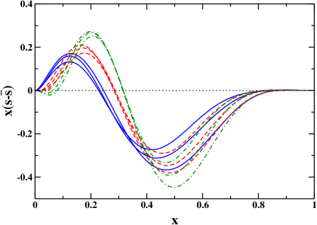
Figure 5: Simultaneous plot of all total $x(s(x)-\bar{s}(x))$ distributions presented in Fig. 4 which are corresponding to the different values of cutoff parameters $\Lambda$.

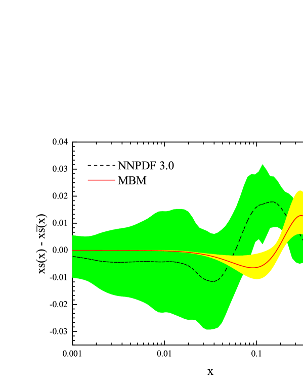
Figure 6: A comparison between the theoretical result of MBM and phenomenologically obtained result of NNPDF3.0 [5] for $s-\bar{s}$ asymmetry. See text for further details.

4 The evolution of the $s-\bar{s}$ asymmetry

Having the total $x(s(x)-\bar{s}(x))$ distribution in the proton obtained in the previous section, we are now ready to study its evolution and then the behaviour of this asymmetry at higher $Q^{2}$. It is well known that the evolution of PDFs is governed by the DGLAP integro-differential equations [89]. Actually, if we have the parton densities as functions of $x$ at an initial scale $\mu_{0}^{2}$, we can obtain them at any arbitrary scale $Q^{2}$ by solving the DGLAP equations. Overall, these equations can be divided into two general parts: singlet and non-singlet equations. A unique feature of the non-singlet equations is that the evolution of a non-singlet distribution is independent of other patron densities and can be carried out solely. In this way, since the $x(s(x)-\bar{s}(x))$ is a non-singlet distribution, we can evolve it to an arbitrary scale $Q^{2}$ no need to other PDFs. The evolution can be performed by the QCDNUM package [101] both in fixed flavor number scheme and variable flavor number scheme. For our case (the evolution of the non-singlet distribution $x(s-\bar{s})$), the only deference between these two schemes is in their procedure to deal with the number of active flavors $n_{f}$ in the evolution of the strong coupling constant $\alpha_{s}$. To be more precise, in FFNS, $n_{f}$ is kept fixed throughout the evolution, while in VFNS, the flavor thresholds $\mu_{c,b,t}^{2}$ related to charm, bottom and top quark masses are introduced and the value of number of active flavors is changed from $n_{f}$ to $n_{f}+1$ at these thresholds (note that the number of active flavors is set to $n_{f}=3$ below the charm threshold).

In other to study the evolution of $x(s(x)-\bar{s}(x))$ in the proton, we select the distribution obtained with $\Lambda_{p}=4$ and $\Lambda_{K}=\Lambda_{\Lambda}=2$ (see the previous section) and evolve it to $Q^{2}=16$ GeV² as an example. The evolution is preformed from two values of initial scale $\mu_{0}=0.3$ and 0.5 GeV as suggested by Chang and Pang in Refs. [35, 36, 37] and at both NLO and NNLO. Moreover, we present the results for both FFNS and VFNS to study the effect of chosen evolution scheme on the behaviour and also magnitude of evolved $x(s(x)-\bar{s}(x))$ distribution. It is worth noting that in all calculations, the value of strong coupling constant at $Z$ boson mass scale ($\alpha_{s}(M_{Z})$) is taken to be 0.118.

Fig. 7 shows the results for $x(s(x)-\bar{s}(x))$ at $Q^{2}=16$ GeV² using FFNS with $n_{f}=5$. The black solid, red dashed, green long-dashed, and blue dotted-dashed curves are related to NLO with $\mu_{0}=0.3$ GeV, NLO with $\mu_{0}=0.5$ GeV, NNLO with $\mu_{0}=0.3$ GeV and NNLO with $\mu_{0}=0.5$ GeV, respectively. As a first conclusion, by comparing Fig. 4 (see red dashed curve in middle panel) and 7, we can see that the distributions have been decreased in magnitude and also shifted to the smaller $x$ due to the evolution. Another conclusion is that the results related to $\mu_{0}=0.5$ GeV have a larger magnitude than $\mu_{0}=0.3$ GeV. Meanwhile, note that there is no considerable deference between the NLO and NNLO results in FFNS.

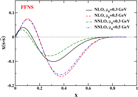
Figure 7: The $x(s(x)-\bar{s}(x))$ distribution in the proton obtained using the Pumplin model and evolved from $\mu_{0}=0.3$ and 0.5 GeV to $Q^{2}=16$ GeV² at NLO and NNLO approximation using FFNS with $n_{f}=5$.

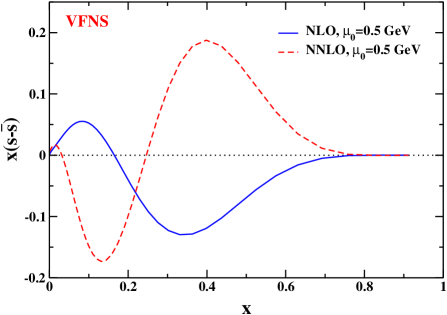
Figure 8: The $x(s(x)-\bar{s}(x))$ distribution in the proton obtained using the Pumplin model and evolved from $\mu_{0}=0.5$ GeV to $Q^{2}=16$ GeV² at NLO and NNLO approximation using VFNS.

The results for $x(s(x)-\bar{s}(x))$ at $Q^{2}=16$ GeV² using VFNS have been shown in Fig. 8. As can be seen, this figure includes only the NLO (blue solid curve) and NNLO (red dashed curve) distributions for $\mu_{0}=0.5$ GeV. Actually, since the value of $\alpha_{s}$ becomes very large at both NLO and NNLO evolution using VFNS with $\mu_{0}=0.3$ GeV, one gets a runtime error in QCDNUM package preventing the program to continue computation. By comparing Figs. 7 and 8, we can see that, at NLO, the $x(s(x)-\bar{s}(x))$ distribution evolved using VFNS behaves as one evolved using FFNS, but with a smaller magnitude in all range of $x$. A very surprising point can be raised from Fig. 8 is that, at NNLO, the $x(s(x)-\bar{s}(x))$ distribution evolved using VFNS behaves quite different compared with one evolved using FFNS (and also with one evolved using VFNS at NLO). In fact, in this case, the position of positive and negative regions in $x(s(x)-\bar{s}(x))$ distribution has been exchanged due to the evolution. This finding suggests that something is wrong, so that the result can be considered unphysical. In other to further investigation on this issue, a good idea is using another package for evolving the $x(s(x)-\bar{s}(x))$ distribution such as the PEGASUS [102].

Fig 9 shows a comparison between the QCDNUM and PEGASUS results for the evolution of the $x(s(x)-\bar{s}(x))$ distribution from different initial scales $\mu_{0}$ to $Q^{2}=16$ GeV² using the VFNS at NNLO. As can be seen, for the case of QCDNUM, if one chooses a value grater than 0.5 GeV for initial scale $\mu_{0}$, for example $\mu_{0}=$ 0.51 (red short-dashed curve), 0.7 (blue long-dashed curve) and 1 GeV (green dotted-dashed curve), the result of evolution will be natural too using VFNS at NNLO. However, when we choose exactly $\mu_{0}=0.5$ GeV, the result is changed dramatically. For a smaller value than 0.5 GeV (even $\mu_{0}=0.49$ GeV), one gets the runtime error due to excessive increase in the value of $\alpha_{s}$. For the case of PEGASUS, the situation is a bit different. Actually, for $\mu_{0}=$ 0.7 and 1 GeV, the QCDNUM and PEGASUS have same results. But, for $\mu_{0}=$ 0.51 GeV, their result is absolutely different. To be more precise, in this scale, the result of QCDNUM seems still natural, but it is clear that the result of PEGASUS is unphysical. It should be noted that the result of PEGASUS for exactly $\mu_{0}=$ 0.5 GeV has not been shown in Fig 9. In fact, in that scale, the value of $\alpha_{s}$ in the PEGASUS calculations becomes infinity, so the program returns a “NaN” value for the $x(s-\bar{s})$ in all $x$. This dramatical behaviour of $x(s-\bar{s})$ distribution under the evolution using the VFNS at NNLO from a very lower initial scale, can be attributed to the excessive increase in the value of $\alpha_{s}$, or maybe has another reason should be carefully investigated in the future researches. Anyhow, the conclusion we can take with certainty from the results obtained in this section is that the choice of initial scale $\mu_{0}$ is a very important ingredient in this respect, and the evolution of the intrinsic quark distributions from a low initial scale, as suggested by Chang and Pang [35, 36, 37], is not a good choice at NNLO using VFNS.

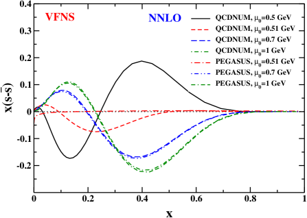
Figure 9: The $x(s(x)-\bar{s}(x))$ distribution in the proton obtained using the Pumplin model and evolved from different initial scales $\mu_{0}$ to $Q^{2}=16$ GeV² at NNLO approximation using VFNS by two packages QCDNUM [101] and PEGASUS [102].

5 Summary and conclusions

One of the most powerful models can lead to $s-\bar{s}$ asymmetry in the nucleon is the meson-baryon model (MBM). According to the MBM formalism, we can consider that the wave function of the nucleon is a series involving bare nucleon and meson-baryon states. It can be shown that, among the possible states, only two states $K^{+}\Lambda^{0}$ and $K^{*+}\Lambda^{0}$ lead to the different shapes for $s$ and $\bar{s}$ distributions in the nucleon and thus the $s-\bar{s}$ asymmetry [34]. Although the MBM formalism is rather complicated computationally, Pumplin [59] has introduced a more simple configuration based on original concepts of this model and used it, for the first time, for the calculation of the intrinsic charm in the nucleon. In Pumplin model, the quantity plays an important role is the cutoff parameter $\Lambda$, so that its chosen value can change the final results. In this way, we can consider a theoretical uncertainty on the distributions due to the $\Lambda$ variation. In this work, we calculated the $s-\bar{s}$ asymmetry for different values of $\Lambda$ to study the dependence of the model to this parameter and also to estimate the theoretical uncertainty imposed on the results due to its uncertainty. As a result, we found that the $x(s(x)-\bar{s}(x))$ distribution resulted from $K^{+}\Lambda^{0}$ state, both in shape and magnitude is very sensitive to value of $\Lambda$, while the related result from $K^{*+}\Lambda^{0}$ state is not very sensitive to it. Then, we calculated the total $x(s(x)-\bar{s}(x))$ distribution in the proton by summing the results obtained for $K^{+}\Lambda^{0}$ and $K^{*+}\Lambda^{0}$ states. We concluded that they decrease in magnitude as $\Lambda_{p}$ decreases. Moreover, for a fixed value of $\Lambda_{p}$, as $\Lambda_{K}=\Lambda_{\Lambda}$ increases, the magnitude of the total distribution somewhat decreases and shifts slightly toward smaller $x$. By comparing all distributions obtained simultaneously, we found that the theoretical uncertainty of the $s-\bar{s}$ asymmetry due to the variation of the cutoff parameters $\Lambda$ is comparatively large in all regions of momentum fraction $x$. However, by calculating exactly the uncertainty of $x(s(x)-\bar{s}(x))$ distribution, we showed that there is a satisfying agreement between the theoretically prediction of MBM and the phenomenologically obtained result of NNPDF3.0, if one considers only the $K^{+}\Lambda^{0}$ state. We also studied the evolution of $x(s(x)-\bar{s}(x))$ distribution both at NLO and NNLO using different evolution schemes. The evolution preformed from different initial scales $\mu_{0}$. As a result, we found that the distributions are decreased in magnitude and also shifted to the smaller $x$ due to the evolution using FFNS. Furthermore, the results related to $\mu_{0}=0.5$ GeV have a larger magnitude than $\mu_{0}=0.3$ GeV and there is no considerable deference between the NLO and NNLO results in FFNS. By comparing the results of FFNS and VFNS, it was found that the evolved $x(s(x)-\bar{s}(x))$ distribution using VFNS at NLO behaves as one evolved using FFNS, but with a smaller magnitude in all range of $x$. Nevertheless, by performing the evolution of the $x(s(x)-\bar{s}(x))$ distribution using VFNS at NNLO through two packages QCDNUM and PEGASUS and comparing their results, we concluded that the choice of initial scale $\mu_{0}$ is a very important ingredient in this respect. To be more precise, at NNLO and using VFNS with $\mu_{0}=$ 0.5 GeV, the result of QCDNUM behaves quite different compared with one evolved using FFNS (and also with one evolved using VFNS at NLO), and using the PEGASUS, one gets a “NaN” value for $x(s-\bar{s})$ distribution in all $x$. This dramatical behaviour can be attributed to the excessive increase in the value of $\alpha_{s}$, or maybe has another reason should be carefully investigated in the future researches. However, the conclusion we can take with certainty from the results obtained is that the evolution of the intrinsic quark distributions from a low initial scale, as suggested by Chang and Pang [35, 36, 37], is not a good choice at NNLO using VFNS.

References

References

- [1] J. C. Collins, D. E. Soper and G. F. Sterman, “Factorization of Hard Processes in QCD,” Adv. Ser. Direct. High Energy Phys. 5, 1 (1989).
- [2] R. Brock et al. [CTEQ Collaboration], “Handbook of perturbative QCD: Version 1.0,” Rev. Mod. Phys. 67, 157 (1995).
- [3] S. Alekhin, J. Blumlein and S. Moch, “The ABM parton distributions tuned to LHC data,” Phys. Rev. D 89, no. 5, 054028 (2014).
- [4] A. Accardi, L. T. Brady, W. Melnitchouk, J. F. Owens and N. Sato, “Constraints on large- parton distributions from new weak boson production and deep-inelastic scattering data,” Phys. Rev. D 93, no. 11, 114017 (2016).
- [5] R. D. Ball et al. [NNPDF Collaboration], “Parton distributions for the LHC Run II,” JHEP 1504, 040 (2015).
- [6] L. A. Harland-Lang, A. D. Martin, P. Motylinski and R. S. Thorne, “Parton distributions in the LHC era: MMHT 2014 PDFs,” Eur. Phys. J. C 75, no. 5, 204 (2015).
- [7] P. Jimenez-Delgado and E. Reya, “Delineating parton distributions and the strong coupling,” Phys. Rev. D 89, no. 7, 074049 (2014).
- [8] S. Dulat et al., “New parton distribution functions from a global analysis of quantum chromodynamics,” Phys. Rev. D 93, no. 3, 033006 (2016).
- [9] A. Aleedaneshvar, M. Goharipour and S. Rostami, “Uncertainty of parton distribution functions due to physical observables in a global analysis,” Chin. Phys. C 41, no. 2, 023101 (2017).
- [10] S. Alekhin, J. Blümlein, S. Moch and R. Placakyte, “Parton distribution functions, , and heavy-quark masses for LHC Run II,” Phys. Rev. D 96, no. 1, 014011 (2017).
- [11] R. D. Ball et al. [NNPDF Collaboration], “Parton distributions from high-precision collider data,” Eur. Phys. J. C 77, no. 10, 663 (2017).
- [12] S. M. Moosavi Nejad, H. Khanpour, S. Atashbar Tehrani and M. Mahdavi, “QCD analysis of nucleon structure functions in deep-inelastic neutrino-nucleon scattering: Laplace transform and Jacobi polynomials approach,” Phys. Rev. C 94, no. 4, 045201 (2016).
- [13] H. Khanpour, A. Mirjalili and S. Atashbar Tehrani, “Analytic derivation of the next-to-leading order proton structure function based on the Laplace transformation,” Phys. Rev. C 95, no. 3, 035201 (2017).
- [14] P. Jimenez-Delgado et al. [Jefferson Lab Angular Momentum (JAM) Collaboration], “Constraints on spin-dependent parton distributions at large x from global QCD analysis,” Phys. Lett. B 738, 263 (2014).
- [15] N. Sato et al. [Jefferson Lab Angular Momentum Collaboration], “Iterative Monte Carlo analysis of spin-dependent parton distributions,” Phys. Rev. D 93, no. 7, 074005 (2016).
- [16] F. Taghavi-Shahri, H. Khanpour, S. Atashbar Tehrani and Z. Alizadeh Yazdi, “Next-to-next-to-leading order QCD analysis of spin-dependent parton distribution functions and their uncertainties: Jacobi polynomials approach,” Phys. Rev. D 93, no. 11, 114024 (2016).
- [17] H. Khanpour, S. T. Monfared and S. Atashbar Tehrani, “Nucleon spin structure functions at NNLO in the presence of target mass corrections and higher twist effects,” Phys. Rev. D 95, no. 7, 074006 (2017).
- [18] J. J. Ethier, N. Sato and W. Melnitchouk, “First simultaneous extraction of spin-dependent parton distributions and fragmentation functions from a global QCD analysis,” Phys. Rev. Lett. 119, no. 13, 132001 (2017).
- [19] H. Khanpour, S. T. Monfared and S. Atashbar Tehrani, “Study of spin-dependent structure functions of and at NNLO approximation and corresponding nuclear corrections,” Phys. Rev. D 96, no. 7, 074037 (2017).
- [20] M. Salajegheh, S. M. Moosavi Nejad, H. Khanpour and S. Atashbar Tehrani, “Analytical approaches to the determination of spin-dependent parton distribution functions at NNLO approximation,” arXiv:1801.04471 [hep-ph].
- [21] K. Kovarik et al., “nCTEQ15 - Global analysis of nuclear parton distributions with uncertainties in the CTEQ framework,” Phys. Rev. D 93, no. 8, 085037 (2016).
- [22] H. Khanpour and S. Atashbar Tehrani, “Global Analysis of Nuclear Parton Distribution Functions and Their Uncertainties at Next-to-Next-to-Leading Order,” Phys. Rev. D 93, no. 1, 014026 (2016).
- [23] K. J. Eskola, P. Paakkinen, H. Paukkunen and C. A. Salgado, “EPPS16: Nuclear parton distributions with LHC data,” Eur. Phys. J. C 77, no. 3, 163 (2017).
- [24] M. Klasen, K. Kovarik and J. Potthoff, “Nuclear parton density functions from jet production in DIS at the EIC,” Phys. Rev. D 95, 094013 (2017).
- [25] R. Wang, X. Chen and Q. Fu, “Global study of nuclear modifications on parton distribution functions,” Nucl. Phys. B 920, 1 (2017).
- [26] S. M. Moosavi Nejad, M. Soleymaninia and A. Maktoubian, “Proton fragmentation functions considering finite-mass corrections,” Eur. Phys. J. A 52, no. 10, 316 (2016).
- [27] E. Leader, A. V. Sidorov and D. B. Stamenov, “Determination of the fragmentation functions from an NLO QCD analysis of the HERMES data on pion multiplicities,” Phys. Rev. D 93, no. 7, 074026 (2016).
- [28] D. de Florian, M. Epele, R. J. Hernandez-Pinto, R. Sassot and M. Stratmann, “Parton-to-Kaon Fragmentation Revisited,” Phys. Rev. D 95, 094019 (2017).
- [29] M. Soleymaninia, H. Khanpour and S. M. Moosavi Nejad, “First determination of -meson fragmentation functions and their uncertainties at next-to-next-to-leading order,” arXiv:1711.11344 [hep-ph].
- [30] S. Catani, D. de Florian, G. Rodrigo and W. Vogelsang, “Perturbative generation of a strange-quark asymmetry in the nucleon,” Phys. Rev. Lett. 93, 152003 (2004).
- [31] M. Salajegheh, H. Khanpour and S. M. Moosavi Nejad, “Improved determination of flavor asymmetry in the proton by BONuS experiment at JLAB and using an approach by Brodsky, Hoyer, Peterson, and Sakai,” Phys. Rev. C 96, no. 6, 065205 (2017).
- [32] S. Kumano, “Flavor asymmetry of anti-quark distributions in the nucleon,” Phys. Rept. 303, 183 (1998).
- [33] W. C. Chang and J. C. Peng, “Flavor Structure of the Nucleon Sea,” Prog. Part. Nucl. Phys. 79, 95 (2014).
- [34] M. Salajegheh, “Intrinsic strange distributions in the nucleon from the light-cone models,” Phys. Rev. D 92, no. 7, 074033 (2015).
- [35] W. C. Chang and J. C. Peng, “Flavor Asymmetry of the Nucleon Sea and the Five-Quark Components of the Nucleons,” Phys. Rev. Lett. 106, 252002 (2011).
- [36] W. C. Chang and J. C. Peng, “Extraction of Various Five-Quark Components of the Nucleons,” Phys. Lett. B 704, 197 (2011).
- [37] W. C. Chang and J. C. Peng, “Extraction of the intrinsic light-quark sea in the proton,” Phys. Rev. D 92, no. 5, 054020 (2015).
- [38] P. H. Beauchemin, V. A. Bednyakov, G. I. Lykasov and Y. Y. Stepanenko, “Search for intrinsic charm in vector boson production accompanied by heavy flavor jets,” Phys. Rev. D 92, no. 3, 034014 (2015).
- [39] F. Lyonnet, A. Kusina, T. Ježo, K. Kovarík, F. Olness, I. Schienbein and J. Y. Yu, “On the intrinsic bottom content of the nucleon and its impact on heavy new physics at the LHC,” JHEP 1507, 141 (2015).
- [40] S. J. Brodsky, A. Kusina, F. Lyonnet, I. Schienbein, H. Spiesberger and R. Vogt, “A review of the intrinsic heavy quark content of the nucleon,” Adv. High Energy Phys. 2015, 231547 (2015).
- [41] A. Aleedaneshvar, M. Goharipour and S. Rostami, “The impact of intrinsic charm on the parton distribution functions,” Eur. Phys. J. A 52, no. 12, 352 (2016).
- [42] S. Rostami, M. Goharipour and A. Aleedaneshvar, “Role of the intrinsic charm content of the nucleon from various light-cone models on γ+c-jet production,” Chin. Phys. C 40, no. 12, 123104 (2016).
- [43] C. S. An and B. Saghai, “Intrinsic light and strange quark–antiquark pairs in the proton and nonperturbative strangeness suppression,” Phys. Rev. D 95, no. 7, 074015 (2017).
- [44] T. J. Hou et al., “CT14 Intrinsic Charm Parton Distribution Functions from CTEQ-TEA Global Analysis,” JHEP 1802, 059 (2018).
- [45] V. A. Bednyakov, S. J. Brodsky, A. V. Lipatov, G. I. Lykasov, M. A. Malyshev, J. Smiesko and S. Tokar, “Constraints on the intrinsic charm content of the proton from recent ATLAS data,” arXiv:1712.09096 [hep-ph].
- [46] S. J. Brodsky, P. Hoyer, C. Peterson and N. Sakai, “The Intrinsic Charm of the Proton,” Phys. Lett. 93B, 451 (1980); S. J. Brodsky, C. Peterson and N. Sakai, “Intrinsic Heavy Quark States,” Phys. Rev. D 23, 2745 (1981).
- [47] A. I. Signal and A. W. Thomas, “Possible Strength of the Nonperturbative Strange Sea of the Nucleon,” Phys. Lett. B 191, 205 (1987).
- [48] S. J. Brodsky and B. Q. Ma, “The Quark / anti-quark asymmetry of the nucleon sea,” Phys. Lett. B 381, 317 (1996).
- [49] H. Holtmann, A. Szczurek and J. Speth, “Flavor and spin of the proton and the meson cloud,” Nucl. Phys. A 596, 631 (1996).
- [50] H. R. Christiansen and J. Magnin, “Strange / anti-strange asymmetry in the nucleon sea,” Phys. Lett. B 445, 8 (1998).
- [51] F. G. Cao and A. I. Signal, “On the phenomenological analyses of s - anti-s asymmetry in the nucleon sea,” Phys. Rev. D 60, 074021 (1999).
- [52] F. G. Cao and A. I. Signal, “The quark anti-quark asymmetry of the strange sea of the nucleon,” Phys. Lett. B 559, 229 (2003).
- [53] Y. Ding and B. Q. Ma, “Contribution of asymmetric strange-antistrange sea to the Paschos-Wolfenstein relation,” Phys. Lett. B 590, 216 (2004).
- [54] F. G. Cao and A. I. Signal, “The polarized nucleon sea in the meson cloud model,” Int. J. Mod. Phys. A 20, 1855 (2005).
- [55] M. Traini, “Next-to-next-to-leading-order nucleon parton distributions from a light-cone quark model dressed with its virtual meson cloud,” Phys. Rev. D 89, no. 3, 034021 (2014).
- [56] A. Vega, I. Schmidt, T. Gutsche and V. E. Lyubovitskij, “Nonperturbative contribution to the strange-antistrange asymmetry of the nucleon sea,” Phys. Rev. D 93, no. 5, 056001 (2016).
- [57] S. Weinberg, “Phenomenological Lagrangians,” Physica A 96, 327 (1979).
- [58] A. Manohar and H. Georgi, “Chiral Quarks and the Nonrelativistic Quark Model,” Nucl. Phys. B 234, 189 (1984).
- [59] J. Pumplin, “Light-cone models for intrinsic charm and bottom,” Phys. Rev. D 73, 114015 (2006).
- [60] E. J. Eichten, I. Hinchliffe and C. Quigg, “Flavor asymmetry in the light quark sea of the nucleon,” Phys. Rev. D 45, 2269 (1992).
- [61] A. Szczurek, A. J. Buchmann and A. Faessler, “On the flavor structure of the constituent quark,” J. Phys. G 22, 1741 (1996).
- [62] M. Wakamatsu and T. Kubota, “Chiral symmetry and the nucleon structure functions,” Phys. Rev. D 57, 5755 (1998); “Chiral symmetry and the nucleon spin structure functions,” Phys. Rev. D 60, 034020 (1999).
- [63] T. P. Cheng and L. F. Li, “Chiral quark model of nucleon spin flavor structure with SU(3) and axial U(1) breakings,” Phys. Rev. D 57, 344 (1998).
- [64] M. Burkardt and B. Warr, “Chiral symmetry and the charge asymmetry of the s anti-s distribution in the proton,” Phys. Rev. D 45, 958 (1992).
- [65] W. Melnitchouk and M. Malheiro, “Strange asymmetries in the nucleon sea,” Phys. Lett. B 451, 224 (1999).
- [66] M. Wakamatsu, “Light flavor sea quark distributions in the nucleon in the SU(3) chiral quark soliton model. 1. Phenomenological predictions,” Phys. Rev. D 67, 034005 (2003).
- [67] Y. Ding, R. G. Xu and B. Q. Ma, “Effect of asymmetric strange-antistrange sea to the NuTeV anomaly,” Phys. Lett. B 607, 101 (2005).
- [68] H. Nematollahi, M. M. Yazdanpanah and A. Mirjalili, “(Anti-)strange density and contribution of heavy flavor, Fc(2) to the nucleon structure function in the chiral quark model,” Int. J. Mod. Phys. A 27, 1250120 (2012).
- [69] M. Wakamatsu, “Flavor structure of the unpolarized and longitudinally-polarized sea-quark distributions in the nucleon,” Phys. Rev. D 90, no. 3, 034005 (2014).
- [70] X. G. Wang, C. R. Ji, W. Melnitchouk, Y. Salamu, A. W. Thomas and P. Wang, “Constraints on asymmetry of the proton in chiral effective theory,” Phys. Lett. B 762 (2016) 52.
- [71] X. G. Wang, C. R. Ji, W. Melnitchouk, Y. Salamu, A. W. Thomas and P. Wang, “Strange quark asymmetry in the proton in chiral effective theory,” Phys. Rev. D 94, no. 9, 094035 (2016).
- [72] U. Dore, “Physics with charm particles produced in neutrino interactions. A historical recollection,” Eur. Phys. J. H 37, 115 (2012).
- [73] W. M. Alberico, S. M. Bilenky and C. Maieron, “Strangeness in the nucleon: Neutrino - nucleon and polarized electron - nucleon scattering,” Phys. Rept. 358, 227 (2002).
- [74] A. O. Bazarko et al. [CCFR Collaboration], “Determination of the strange quark content of the nucleon from a next-to-leading order QCD analysis of neutrino charm production,” Z. Phys. C 65, 189 (1995).
- [75] D. Mason et al. [NuTeV Collaboration], “Measurement of the Nucleon Strange-Antistrange Asymmetry at Next-to-Leading Order in QCD from NuTeV Dimuon Data,” Phys. Rev. Lett. 99, 192001 (2007).
- [76] A. Kayis-Topaksu et al., “Measurement of charm production in neutrino charged-current interactions,” New J. Phys. 13, 093002 (2011).
- [77] O. Samoylov et al. [NOMAD Collaboration], “A Precision Measurement of Charm Dimuon Production in Neutrino Interactions from the NOMAD Experiment,” Nucl. Phys. B 876, 339 (2013).
- [78] S. Chatrchyan et al. [CMS Collaboration], “Measurement of associated W + charm production in pp collisions at = 7 TeV,” JHEP 1402, 013 (2014).
- [79] G. Aad et al. [ATLAS Collaboration], “Measurement of the production of a boson in association with a charm quark in collisions at 7 TeV with the ATLAS detector,” JHEP 1405, 068 (2014).
- [80] G. P. Zeller et al. [NuTeV Collaboration], “A Precise determination of electroweak parameters in neutrino nucleon scattering,” Phys. Rev. Lett. 88, 091802 (2002) Erratum: [Phys. Rev. Lett. 90, 239902 (2003)].
- [81] B. Q. Ma, “Nutev anomaly versus strange-antistrange asymmetry,” Int. J. Mod. Phys. A 21, 930 (2006).
- [82] P. Gao and B. Q. Ma, “Influence of Heavy Quark Recombination on the Nucleon Strangeness Asymmetry,” Phys. Rev. D 77, 054002 (2008).
- [83] Y. Chi, X. Du and B. Q. Ma, “Nucleon strange asymmetry to the fragmentation,” Phys. Rev. D 90, no. 7, 074003 (2014).
- [84] X. Du and B. Q. Ma, “Strange quark-antiquark asymmetry of nucleon sea from polarization,” Phys. Rev. D 95, no. 1, 014029 (2017).
- [85] V. Barone, C. Pascaud and F. Zomer, “A New global analysis of deep inelastic scattering data,” Eur. Phys. J. C 12, 243 (2000).
- [86] M. Goncharov et al. [NuTeV Collaboration], “Precise measurement of dimuon production cross-sections in muon neutrino Fe and muon anti-neutrino Fe deep inelastic scattering at the Tevatron,” Phys. Rev. D 64, 112006 (2001).
- [87] F. Olness et al., “Neutrino dimuon production and the strangeness asymmetry of the nucleon,” Eur. Phys. J. C 40, 145 (2005).
- [88] W. Bentz, I. C. Cloet, J. T. Londergan and A. W. Thomas, “Reassessment of the NuTeV determination of the weak mixing angle,” Phys. Lett. B 693, 462 (2010).
- [89] V. N. Gribov and L. N. Lipatov, “Deep inelastic e p scattering in perturbation theory,” Sov. J. Nucl. Phys. 15, 438 (1972) [Yad. Fiz. 15, 781 (1972)]; G. Altarelli and G. Parisi, “Asymptotic Freedom in Parton Language,” Nucl. Phys. B 126, 298 (1977); Y. L. Dokshitzer, “Calculation of the Structure Functions for Deep Inelastic Scattering and e+ e- Annihilation by Perturbation Theory in Quantum Chromodynamics.,” Sov. Phys. JETP 46, 641 (1977) [Zh. Eksp. Teor. Fiz. 73, 1216 (1977)].
- [90] W. Melnitchouk and A. W. Thomas, “HERA anomaly and hard charm in the nucleon,” Phys. Lett. B 414, 134 (1997).
- [91] S. Paiva, M. Nielsen, F. S. Navarra, F. O. Duraes and L. L. Barz, “Virtual meson cloud of the nucleon and intrinsic strangeness and charm,” Mod. Phys. Lett. A 13, 2715 (1998).
- [92] T. J. Hobbs, J. T. Londergan and W. Melnitchouk, “Phenomenology of nonperturbative charm in the nucleon,” Phys. Rev. D 89, no. 7, 074008 (2014).
- [93] M. Goharipour and H. Mehraban, “Predictions for the Isolated Prompt Photon Production at the LHC at 13TeV,” Adv. High Energy Phys. 2017, 3802381 (2017).
- [94] M. Goharipour and H. Mehraban, “Study of isolated prompt photon production in -Pb collisions for the ALICE kinematics,” Phys. Rev. D 95, no. 5, 054002 (2017).
- [95] P. Amaudruz et al. [New Muon Collaboration], “The Gottfried sum from the ratio F2(n) / F2(p),” Phys. Rev. Lett. 66, 2712 (1991); M. Arneodo et al. [New Muon Collaboration], “A Reevaluation of the Gottfried sum,” Phys. Rev. D 50, R1 (1994).
- [96] K. Ackerstaff et al. [HERMES Collaboration], “The Flavor asymmetry of the light quark sea from semiinclusive deep inelastic scattering,” Phys. Rev. Lett. 81, 5519 (1998).
- [97] E. A. Hawker et al. [NuSea Collaboration], “Measurement of the light anti-quark flavor asymmetry in the nucleon sea,” Phys. Rev. Lett. 80, 3715 (1998); J. C. Peng et al. [NuSea Collaboration], “Anti-d / anti-u asymmetry and the origin of the nucleon sea,” Phys. Rev. D 58, 092004 (1998); R. S. Towell et al. [NuSea Collaboration], “Improved measurement of the anti-d / anti-u asymmetry in the nucleon sea,” Phys. Rev. D 64, 052002 (2001).
- [98] V. Barone, C. Pascaud, B. Portheault and F. Zomer, “Parton distribution functions in a fit of DIS and related data,” JHEP 0601, 006 (2006).
- [99] A. Ghasempour Nesheli, “The impact of asymmetry on the strange electromagnetic form factor,” Eur. Phys. J. A 52, no. 9, 274 (2016).
- [100] H. Fritzsch, “Quarks and QCD,” Int. J. Mod. Phys. A 29, no. 15, 1430038 (2014).
- [101] M. Botje, “QCDNUM: Fast QCD Evolution and Convolution,” Comput. Phys. Commun. 182, 490 (2011).
- [102] A. Vogt, “Efficient evolution of unpolarized and polarized parton distributions with QCD-PEGASUS,” Comput. Phys. Commun. 170, 65 (2005).