On cold diluted plasmas hit by short laser pulses

Abstract

Abstract:  Adapting a plane hydrodynamical model we briefly revisit the study of the impact of a very short and intense laser pulse onto a diluted plasma, the formation of a plasma wave, its wave-breaking, the occurrence of the slingshot effect.

Keywords:  Laser-plasma interactions; electron acceleration; plasma wave; wave-breaking; slingshot effect

I Introduction

The laser-plasma interactions induced by ultra-intense or ultra-short laser pulses are at the base of the Laser Wake-Field (LWF) Tajima-Dawson1979 and other extremely compact acceleration mechanism of charged particles with extremely important potential applications in medicine, industry, etc. The equations ruling them are so complex that recourse to numerical resolution based on e.g. particle-in-cell (PIC) techniques is almost unavoidable. PIC or other codes in general involve huge and costly computations for each choice of the free parameters; exploring the parameter space blindly to pinpoint the interesting regions is prohibitive, if not accompanied by some analytical insight that can simplify the work, at least in special cases or in a limited space-time region. This applies in particular to the impact of a very intense and short laser pulse (the pump) on a cold diluted plasma (or matter to be locally ionized into a plasma by the pulse itself). Here we briefly revisit it using an improved 1D Lagrangian model: with very little computational power we can more easily determine conditions (on the initial density $\widetilde{n_{0}}$, the laser length $l$ and spot radius $R$) for, and information on: i) the formation of a plasma wave (PW) AkhPol56 ; BulKirSak89 and its breaking Daw59 - if any - at density inhomogeneities BulEtAl98 ; BraEtAl08 ; LiEtAl13 (this is important as a possible injection mechanism for the LWFA); ii) the slingshot effect, i.e. the backward expulsion of a bunch of high-energy electrons from the plasma surface FioFedDeA14 ; FioDeN16 shortly after the impact of the pulse. More detailed arguments will appear in the longer paper Fio17 .

We assume the plasma is initially neutral, unmagnetized and at rest with zero densities in the region  $z\!<\!0$. We describe it as a static background of ions and a fully relativistic collisionless fluid of electrons, with plasma and electric, magnetic fields ${\bf E},{\bf B}$ fulfilling the Lorentz-Maxwell and continuity equations. We check a posteriori where and how long such a hydrodynamical picture is self-consistent. We assume $t\!=\!0$ initial conditions for the electrons Eulerian density $n_{e}$, velocity ${\bf v}_{e}$ of the type

$${\bf v}_{e}(0,\!{\bf x})\!=\!{\bf 0},\qquad n_{e}(0,\!{\bf x})\!=\!\widetilde{n_{0}}(z),\quad\widetilde{n_{0}}(z)\!=\!0\>\>\mbox{if }\>z\!\leq\!0,$$ (1)

where $0\!<\!\widetilde{n_{0}}(z)\!\leq\!n_{b}$ if $z\!>\!0$ and for simplicity $\widetilde{n_{0}}(z)\!=\!n_{0}$ if $z\!\geq\!z_{s}$, for some $n_{b}\!\geq\!n_{0}\!>\!0$, $z_{s}\!\geq\!0$. As we regard ions as immobile, the proton density will be $n_{p}(t,{\bf x})\!=\!\widetilde{n_{0}}(z)$ for all $t$. We assume that the pump can be schematized for $t\!<\!0$ as a free plane transverse wave $\mbox{\boldmath$\epsilon$}^{{\scriptscriptstyle\perp}}\!(ct\!-\!z)$   traveling in the $z$-direction ($\perp$ means orthogonal to $\vec{z}$, $c$ is the speed of light) multiplied by a ‘cutoff’ function $\chi\!_{{\scriptscriptstyle R}}(\rho)$,

$${\bf E}^{\scriptscriptstyle\perp}(t,{\bf x})=\mbox{\boldmath$\epsilon$}^{{\scriptscriptstyle\perp}}\!(ct\!-\!z)\,\chi\!_{{\scriptscriptstyle R}}(\rho),\quad{\bf B}^{{\scriptscriptstyle\perp}}={\hat{\bf z}}\!\times\!{\bf E}^{\scriptscriptstyle\perp}\qquad\mbox{if }t\leq 0;$$ (2)

more precisely, $\chi\!_{{\scriptscriptstyle R}}(\rho)$ is 1 if $\rho\!\equiv\!\sqrt{\!x^{2}\!+\!y^{2}}\!\leq\!R$ and rapidly goes to zero for $\rho\!>\!R$,  while $\mbox{\boldmath$\epsilon$}^{{\scriptscriptstyle\perp}}\!(\xi)\!=\!0$ unless $0\!<\!\xi\!<\!l$, where the effective pulse length $l$ fulfills

$$2l\lesssim ct_{{\scriptscriptstyle H}},$$ (3)

and $t_{{\scriptscriptstyle H}}$ is the plasma period associated to the density $n_{b}$ [see (29) below]. $\mbox{\boldmath$\epsilon$}^{{\scriptscriptstyle\perp}}\!(\xi)\!=\!0$ if $\xi\!<\!0$ means that the pulse reaches the plasma at $t\!=\!0$. Condition (3) secures that the pulse is completely inside the bulk before any electron gets out of it and is fulfilled if $l$ or $n_{b}$ are small enough (a fortiori the plasma is underdense); in particular, if $2l\!\leq\!ct_{{\scriptscriptstyle H}}^{{\scriptscriptstyle nr}}$;  $t_{{\scriptscriptstyle H}}^{{\scriptscriptstyle nr}}\!\equiv\!\sqrt{\pi m/n_{b}e^{2}}\!\leq\!t_{{\scriptscriptstyle H}}$ is the non-relativistic limit of $t_{{\scriptscriptstyle H}}$ ($m,-e$ are the electron mass, charge). As we make no extra assumptions on the Fourier spectrum or the polarization of $\mbox{\boldmath$\epsilon$}^{{\scriptscriptstyle\perp}}$, our method can be applied to all kind of such travelling waves, ranging from almost monochromatic to so called “impulses”.

In section II we discuss the motion of electrons when $R\!=\!\infty$ ($\chi\!_{{\scriptscriptstyle R}}\!\equiv\!1$) using an improved plane hydrodynamical model Fio14JPA ; Fio17JPA (for shorter presentations see FioRev ) that allows to reduce the system of Lorentz-Maxwell and continuity partial differential equations (PDEs) into ordinary differential equations (ODEs), more precisely into a family of decoupled systems of non-autonomous Hamilton Equations in dim 1 in rational form. In the model we alternatively adopt the light-like coordinate  $\xi=ct\!-\!z$  or time $t$ to parametrize the electron motion, the transverse and the light-like components  ${\bf p}^{\scriptscriptstyle\perp}_{e}$, $p_{e}^{0}\!-\!cp_{e}^{z}\!\equiv\!mc^{2}s_{e}$ (instead of the longitudinal one $p_{e}^{z}$) of the electron 4-momentum as unknowns, neglect pump depletion, control how long this is valid, how long the hydrodynamical picture holds, when and where it fails (by wave-breaking Daw59 ). Then we test the model by numerically solving the ODE’s with $\widetilde{n_{0}}(Z)$ either step-like, or as in BraEtAl08 (i.e. linearly growing in a first interval and decreasing in a second), and find consistent results. In section III we use causality and heuristic arguments to qualitatively adapt these results to the “real world” ($R\!<\!\infty$) and justify the above statements.

II Set-up and plane model

The equations of motion of an electron $e^{-}$ is non-autonomous and highly nonlinear in the unknowns the position  ${\bf x}(t)$  and momentum  ${\bf p}(t)=mc\,{\bf u}(t)$:

$$\begin{array}[]{l}\displaystyle\dot{\bf p}(t)=-e{\bf E}[t,{\bf x}(t)]-\frac{{\bf p}(t)\wedge e{\bf B}[t,{\bf x}(t)]}{\sqrt{m^{2}c^{2}\!+\!{\bf p}^{2}(t)}},\\[6.0pt] \displaystyle\frac{\dot{\bf x}(t)}{c}=\frac{{\bf p}(t)}{\sqrt{m^{2}c^{2}\!+\!{\bf p}^{2}(t)}},\end{array}$$ (6)

We decompose ${\bf x}\!=\!x{\bf i}\!+\!y{\bf j}\!+\!z{\bf k}\!={\bf x}^{\scriptscriptstyle\perp}\!+\!z{\bf k}$, etc, in the cartesian coordinates of the laboratory frame, and often use the dimensionless variables $\mbox{\boldmath$\beta$}\!\equiv\!{\bf v}/c\!=\!\dot{\bf x}/c$,   $\gamma\!\equiv\!1/\sqrt{1\!-\!\mbox{\boldmath$\beta$}^{2}}\!=\!\sqrt{1\!+\!{\bf u}^{2}}$,  the 4-velocity $u\!=\!(u^{0}\!,{\bf u})\!\equiv\!(\gamma,\gamma\mbox{\boldmath$\beta$})$, i.e. the dimensionless version of the 4-momentum $p$. As by (6b) $e^{-}$ cannot reach the speed of light,  $\tilde{\xi}(t)\!=\!ct\!-\!z(t)$ grows strictly, and we can make the change $t\mapsto\xi\!=\!ct\!-\!z$ of independent parameter along the worldline of $e^{-}$ (see fig. 2), so that the term $\mbox{\boldmath$\epsilon$}^{\scriptscriptstyle\perp}[ct-z(t)]$, where the unknown $z(t)$ is in the argument of the highly nonlinear and rapidly varying $\mbox{\boldmath$\epsilon$}^{\scriptscriptstyle\perp}$, becomes the known forcing term $\mbox{\boldmath$\epsilon$}^{\scriptscriptstyle\perp}(\xi)$. We denote as $\hat{\bf x}(\xi)$ the position of $e^{-}$ as a function of $\xi$; it is determined by $\hat{\bf x}(\xi)={\bf x}(t)$. More generally we denote $\hat{f}(\xi,\hat{\bf x})\equiv f[(\xi\!+\!\hat{z})/c,\hat{\bf x}]$ for any given function $f(t,{\bf x})$, abbreviate $\dot{f}\!\equiv\!df/dt$, $\hat{f}^{\prime}\!\equiv\!d\hat{f}/d\xi$ (total derivatives). It is convenient to make also the change of dependent (and unknown) variable $u^{z}\!\mapsto\!s$, where the $s$-factor Fio17

$$s\equiv\gamma\!-u^{z}=u^{-}=\gamma(1-\beta^{z})=\frac{\gamma}{c}\frac{d\tilde{\xi}}{dt}>0$$ (7)

is the light-like component of $u$, as well as the Doppler factor of $e^{-}$: $\gamma,{\bf u},\mbox{\boldmath$\beta$}$ are the rational functions of ${\bf u}^{{\scriptscriptstyle\perp}},s$

$$\gamma\!=\!\frac{1\!+\!{\bf u}^{{\scriptscriptstyle\perp}}{}^{2}\!\!+\!s^{2}}{2s},\qquad u^{z}\!=\!\frac{1\!+\!{\bf u}^{{\scriptscriptstyle\perp}}{}^{2}\!\!-\!s^{2}}{2s},\qquad\mbox{\boldmath$\beta$}\!=\!\frac{{\bf u}}{\gamma}$$ (8)

(these relations hold also with the carets); so, replacing $d/dt\mapsto(cs/\gamma)d/d\xi$ and putting carets on all variables (6) becomes rational in the unknowns $\hat{\bf u}^{{\scriptscriptstyle\perp}},\hat{s}$, in particular (6b) becomes $\hat{\bf x}^{\prime}=\hat{\bf u}/\hat{s}$. Moreover, $\hat{s}$ is practically insensitive to fast oscillations of $\mbox{\boldmath$\epsilon$}^{\scriptscriptstyle\perp}(\xi)$ (as e.g. fig. 1b illustrates). Passing to the plasma, we denote as  ${\bf x}_{e}(t,{\bf X})$  the position at time $t$ of the electrons’ fluid element $d^{3}X$ initially located at ${\bf X}\!\equiv\!(X,Y,Z)$, as $\hat{\bf x}_{e}(\xi,{\bf X})$ the position of $d^{3}X$ as a function of $\xi$. For brevity we refer to the electrons initially contained: in $d^{3}X$, as the ‘${\bf X}$ electrons’; in a region $\Omega$, as the ‘$\Omega$ electrons’; in the layer between $Z,Z\!+\!dZ$, as the ‘$Z$ electrons’. The map ${\bf x}_{e}(t,\cdot):{\bf X}\mapsto{\bf x}$ must be one-to-one for every $t$; equivalently, $\hat{\bf x}_{e}(\xi,\cdot):{\bf X}\mapsto{\bf x}$ must be one-to-one for every $\xi$. Clearly,

$${\bf X}_{e}(t,{\bf x})=\hat{\bf X}_{e}(ct\!-\!z,{\bf x}).$$ (9)

In this section we set $\chi\!_{{\scriptscriptstyle R}}\!\equiv\!1$ in (2), so that all initial data are independent of transverse coordinates. Hence, also the Eulerian fields solving the equations will depend only on   $z,t$, thus justifying the Ansatz $A(t,z)$ for the EM potential $A\!=\!(A^{0}\!,\!{\bf A})$. Then the initial condition (2) implies that for all $t$ ${\bf A}\!^{\scriptscriptstyle\perp}$ is a physical observable and

$${\bf A}\!^{{\scriptscriptstyle\perp}}\!(t\!,\!z)\!=\!-c\!\!\!\int\limits^{t}_{-\infty}\!\!\!dt^{\prime}{\bf E}^{\scriptscriptstyle\perp}\!(t{}^{\prime}\!,\!z),\quad c{\bf E}^{\scriptscriptstyle\perp}\!\!=\!-\partial_{t}{\bf A}\!^{\scriptscriptstyle\perp},\quad{\bf B}\!=\!{\bf k}\!\wedge\!\partial_{z}{\bf A}\!^{\scriptscriptstyle\perp}\!.$$ (10)

Similarly, the displacement  $\Delta{\bf x}_{e}\equiv{\bf x}_{e}(t,\!{\bf X}\!)-\!{\bf X}$ will actually depend only on $t,Z$ [and $\Delta\hat{\bf x}_{e}\equiv\hat{\bf x}_{e}(\xi,{\bf X})\!-\!{\bf X}$ only on $\xi,Z$] and by causality vanishes if   $ct\!\leq\!Z$. The Eulerian electrons’ momentum ${\bf p}_{e}(t,z)$ obeys equation (6), where one has to replace ${\bf x}(t)\mapsto{\bf x}_{e}(t,{\bf X})$, $\dot{\bf p}\mapsto d{\bf p}_{e}/dt\equiv$ total derivative; as known, by (10) the transverse part of (6a) becomes $\frac{d{\bf p}^{{\scriptscriptstyle\perp}}_{e}}{dt}=\frac{e}{c}\frac{d{\bf A}\!^{\scriptscriptstyle\perp}}{dt}$, which due to ${\bf p}^{{\scriptscriptstyle\perp}}_{e}(0,{\bf x})={\bf 0}$ implies

$${\bf p}^{{\scriptscriptstyle\perp}}_{e}=\frac{e}{c}{\bf A}\!^{\scriptscriptstyle\perp}\qquad\quad\mbox{i.e. }\quad{\bf u}^{\scriptscriptstyle\perp}_{e}=\frac{e}{mc^{2}}{\bf A}\!^{\scriptscriptstyle\perp}.$$ (11)

Eq. (11), which holds also with the caret, allows to trade ${\bf u}^{\scriptscriptstyle\perp}_{e}$ for ${\bf A}\!^{\scriptscriptstyle\perp}$ as an unknown. From (2) it follows for $t\leq 0$

$${\bf A}\!^{\scriptscriptstyle\perp}(t,z)={\bm{\alpha}}^{\scriptscriptstyle\perp}(ct\!-\!z),\qquad{\bm{\alpha}}^{\scriptscriptstyle\perp}(\xi)\!\equiv\!-\!\!\int^{\xi}_{-\infty}\!\!\!d\eta\>\mbox{\boldmath$\epsilon$}^{\scriptscriptstyle\perp}(\eta).$$ (12)

The local conservation  $n_{e}\,dz=\widetilde{n_{0}}\,dZ$  of the number of electrons (whence the continuity equation) becomes

$$n_{e}(t,z)=\widetilde{n_{0}}\!\left[Z_{e}(t,\!z)\right]\,\partial_{z}Z_{e}(t,z),$$ (13)

and the Maxwell equations  $\nabla\!\!\cdot\!{\bf E}\!-\!4\pi j^{0}\!=\!\partial_{z}E^{z}\!-4\pi e(n_{p}-n_{e})\!=\!0$,  $\partial_{t}E^{z}/c\!\!+\!4\pi j^{z}\!\!=\!(\nabla\!\!\wedge\!{\bf B})^{z}\!\!=\!0$ (${\bf j}\!=\!-en_{e}\mbox{\boldmath$\beta$}_{e}$ is the current density) with the initial conditions imply Fio14JPA

$$E^{z}(t,\!z)\!=\!4\pi e\!\left\{\widetilde{N}(z)\!-\!\widetilde{N}[Z_{e}(t,\!z)]\right\}\!,\>\>\>\widetilde{N}(Z)\!\equiv\!\!\!\int^{Z}_{0}\!\!\!\!\!\!d\eta\,\widetilde{n_{0}}(\eta).$$ (14)

Relations (13-14) allow to compute $n_{e},E^{z}$ explicitly in terms of the assigned initial density $\widetilde{n_{0}}$ and of the still unknown $Z_{e}(t,z)$ (longitudinal motion); thereby they further reduce the number of unknowns. The remaining ones are ${\bf A}\!^{{\scriptscriptstyle\perp}},{\bf x}_{e}$ and $u_{e}^{z}$, or - equivalently - $s_{e}$.

Using the Green function of $\frac{1}{c^{2}}\partial_{t}^{2}\!-\!\partial_{z}^{2}$ one finds that the Maxwell equation  $\Box{\bf A}\!^{\scriptscriptstyle\perp}=4\pi{\bm{j}}^{\scriptscriptstyle\perp}$ (in the Landau gauges) & (12) amount to the integral equation Fio14JPA

$$\begin{array}[]{ll}\displaystyle{\bf A}\!^{{\scriptscriptstyle\perp}}(t,z)-{\bm{\alpha}}^{\scriptscriptstyle\perp}(ct\!-\!z)=&\!\!\!\displaystyle-\frac{2\pi e^{2}}{mc^{2}}\!\!\!\int\!\!\!d\eta d\zeta\left(\!\frac{n_{e}{\bf A}\!^{\scriptscriptstyle\perp}}{\gamma_{e}}\!\right)\!\left(\eta,\zeta\right)\\[8.0pt] &\displaystyle\times\,\theta(\eta)\,\theta\left(ct\!-\!\eta\!-\!|z\!-\!\zeta|\right).\end{array}$$ (15)

Abbreviating   $v\!\equiv\!\hat{\bf u}^{{\scriptscriptstyle\perp}}_{e}{}^{2}\!=\![e\hat{\bf A}\!^{{\scriptscriptstyle\perp}}/{mc^{2}}]^{2}$,  $\hat{\Delta}(\xi,Z)\!\equiv\!\hat{z}_{e}(\xi,Z)\!-\!Z$,  the remaining eq.s (6) take the form $\hat{\bf x}^{{\scriptscriptstyle\perp}}_{e}{}^{\prime}\!=\!\hat{\bf u}^{{\scriptscriptstyle\perp}}_{e}/\hat{s}_{e}$ and

$$\hat{\Delta}^{\prime}\!=\displaystyle\frac{1\!+\!v}{2\hat{s}_{e}^{2}}\!-\!\frac{1}{2},\quad\hat{s}^{\prime}_{e}(\xi,\!Z)\!=\!\frac{4\pi e^{2}}{mc^{2}}\!\left\{\widetilde{N}\left[Z\!+\!\hat{\Delta}\right]\!-\!\widetilde{N}(Z)\right\}\!,$$ (16)

with initial conditions  $\hat{\Delta}(-Z,\!Z)\!=\!0$, $\hat{s}(-Z,\!Z)\!=\!1$. Eq.s (16) prevent $\hat{s}_{e}$ to vanish anywhere, consistently with (7): if $\hat{s}_{e}\!\downarrow\!0$ then rhs(16a) blows up and forces $\hat{\Delta}$, and in turn $\hat{s}_{e}\!-\!1$, to abruptly grow again positive. By causality ${\bf A}\!^{{\scriptscriptstyle\perp}}(t,z)\!=\!0$ if $ct\!\leq\!z$, hence $v,\hat{\Delta},\hat{s}_{e}-1$ remain zero until $\xi\!=\!0$, and we can shift the initial conditions to

$$\hat{\Delta}(0,\!Z)\!=\!0,\qquad\qquad\hat{s}_{e}(0,\!Z)\!=\!1.$$ (17)

Moreover, as the right-hand side (rhs) of (15) is zero for $t\leq 0$, we can still use (12), and by (11) approximate   $\hat{\bf u}^{{\scriptscriptstyle\perp}}_{e}\!=\!e{\bm{\alpha}}^{\scriptscriptstyle\perp}/{mc^{2}}$, within short time intervals $[0,t_{s}]$ (to be determined a posteriori); $\hat{\bf u}^{{\scriptscriptstyle\perp}}_{e}$ and the forcing term $v$ thus become known functions of $\xi$ (only), and (16) a family parametrized by $Z$ of decoupled ODEs. For every $Z$ (16) have the form of Hamilton equations  $q^{\prime}=\partial\hat{H}/\partial p$, $p^{\prime}=-\partial\hat{H}/\partial q$ of a 1-dim system:   $\xi,\hat{\Delta},-\hat{s}_{e}$ play the role of $t,q,p$, and the Hamiltonian is rational in $\hat{s}_{e}$ and reads

$$\begin{array}[]{l}\displaystyle\hat{H}(\hat{\Delta},\hat{s}_{e},\xi;Z)\equiv\frac{\hat{s}_{e}^{2}+1\!+\!v(\xi)}{2\hat{s}_{e}}+{\cal U}(\hat{\Delta};Z),\\[8.0pt] {\cal U}(\Delta;Z)\!\equiv\!\frac{4\pi e^{2}}{mc^{2}}\left[\widetilde{{\cal N}}\!\left(Z\!+\!\Delta\right)\!-\!\widetilde{{\cal N}}\!(Z)\!-\!\widetilde{N}\!(Z)\hat{\Delta}\right],\\[8.0pt] \displaystyle\widetilde{{\cal N}}(Z)\equiv\int^{Z}_{0}\!\!\!d\zeta\,\widetilde{N}(\zeta)\!=\!\int^{Z}_{0}\!\!\!d\zeta\,\widetilde{n_{0}}(\zeta)\,(Z\!-\!\zeta).\end{array}$$ (21)

Eq.s (16-17) can be solved numerically, or by quadrature where $\mbox{\boldmath$\epsilon$}^{\scriptscriptstyle\perp}(\xi)\!=\!0$. Finally  $\hat{\bf x}^{{\scriptscriptstyle\perp}}_{e}{}^{\prime}\!=\!\hat{\bf u}^{{\scriptscriptstyle\perp}}_{e}/\hat{s}_{e}$ is solved by

$$\hat{\bf x}^{\scriptscriptstyle\perp}_{e}(\xi,{\bf X})-{\bf X}^{\scriptscriptstyle\perp}=\!\int^{\xi}_{0}\!\!\!d\eta\,\frac{\hat{\bf u}^{\scriptscriptstyle\perp}_{e}(\eta)}{\hat{s}(\eta,Z)}.$$ (22)

By derivation we obtain several useful relations, e.g.

$$\frac{\partial Z_{e}}{\partial z}(t,z)=\left.\frac{\hat{\gamma}_{e}}{\hat{s}_{e}\,\partial_{Z}\hat{z}_{e}}\right|_{(\xi,Z)=\big{(}ct\!-z,Z_{e}(t,z)\big{)}}.$$ (23)

Hence the maps  $\hat{\bf x}_{e}(\xi,\cdot)\!:\!{\bf X}\!\mapsto\!{\bf x}$,  ${\bf x}_{e}(t,\cdot)\!:\!{\bf X}\!\mapsto\!{\bf x}$  are invertible, and the hydrodynamic approach justified, as long as $\partial_{Z}\hat{z}_{e}\!>\!0$.  From (13), (23)

$$n_{e}(t,z)\!=\!\left.\frac{\hat{\gamma}_{e}\,\widetilde{n_{0}}}{\hat{s}_{e}\,\partial_{Z}\hat{z}_{e}}\right|_{(\xi,Z)=\big{(}ct\!-z,Z_{e}(t,z)\big{)}}.$$ (24)

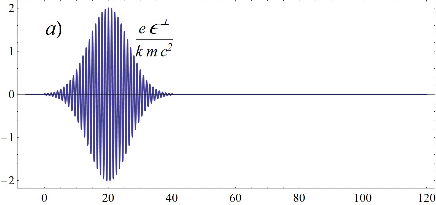
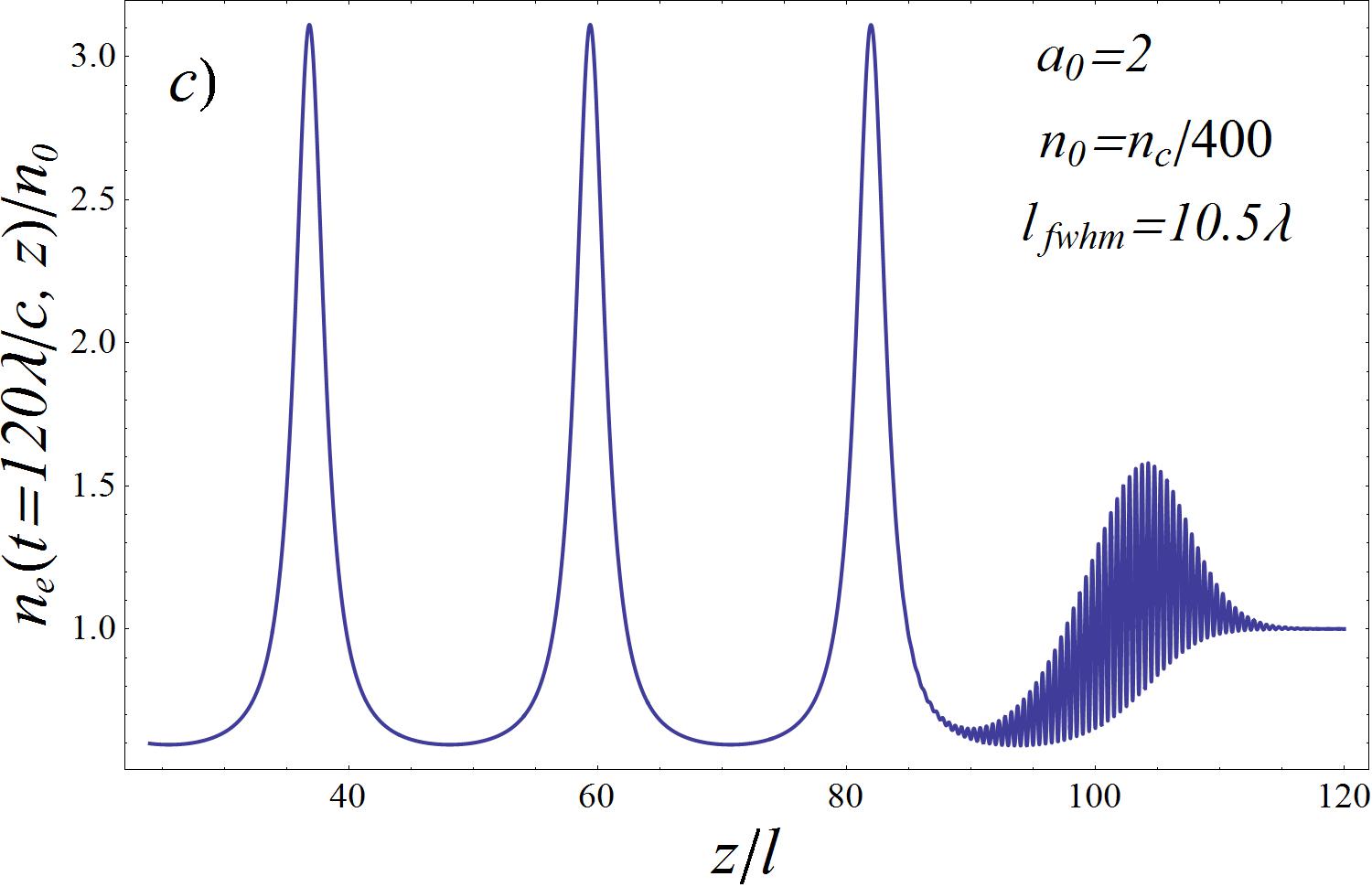
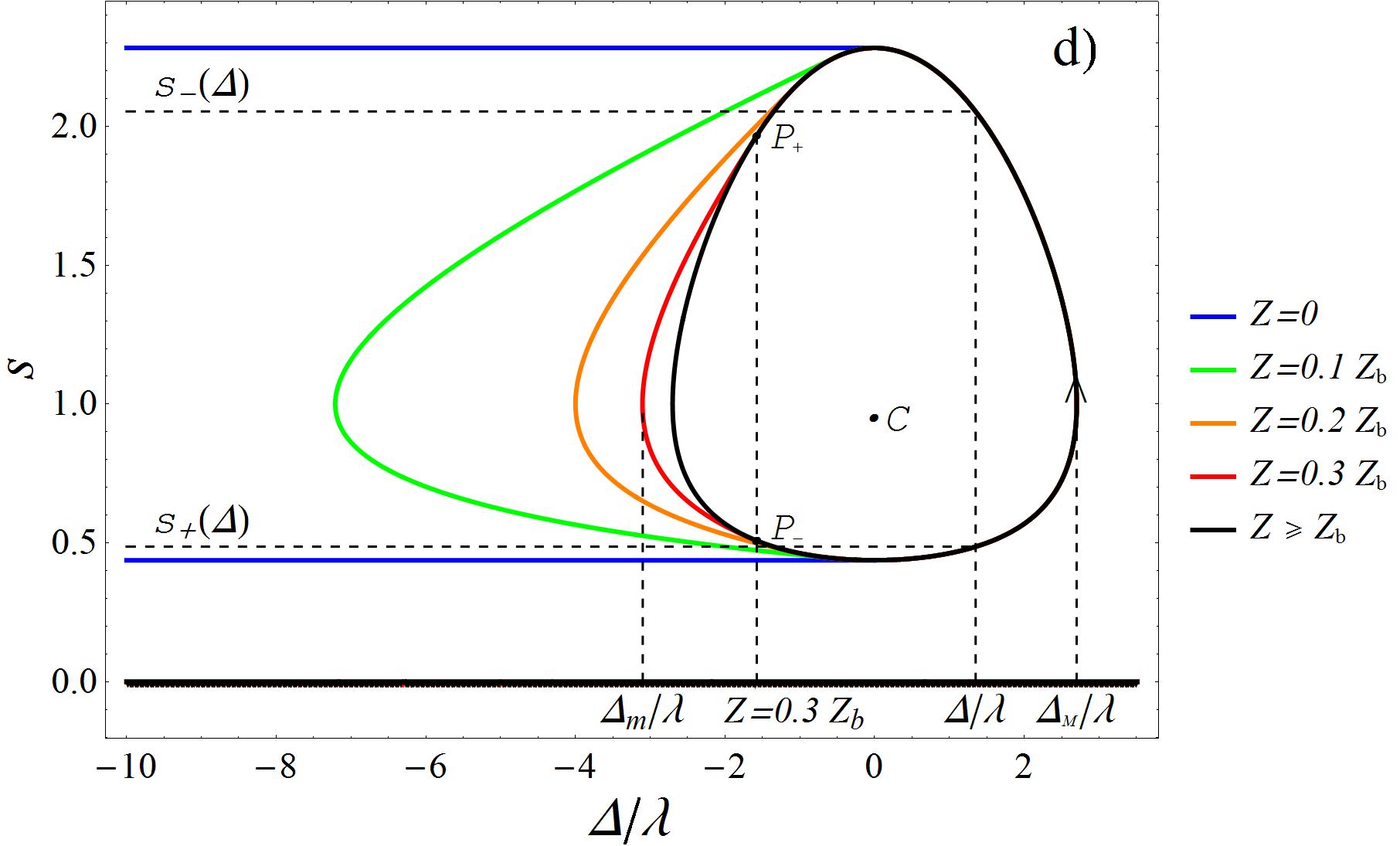
Figure 1: (Color online)  a) Normalized gaussian pump of length $l_{fwhm}\!=\!10.5\lambda$, linear polarization, peak amplitude $a_{0}\!\equiv\!2\pi eE^{\scriptscriptstyle\perp}_{\scriptscriptstyle M}/mc^{2}k\!=\!2$ (leading to a peak intensity $I\!=\!1.7\!\times\!10^{19}$W/cm² if $\lambda=0.8\mu$m).   b)  Corresponding solution of (30-17) for $Z\!\geq\!Z_{d}$, with $\widetilde{n_{0}}(Z)\!=\!n_{0}\theta(Z)$, $n_{0}\!\equiv\!n_{cr}/400$ (whence $h\!=\!1.36$); as anticipated, $\hat{s}$ is indeed insensitive to fast oscillations of $\mbox{\boldmath$\epsilon$}^{\scriptscriptstyle\perp}$.  c)  Corresponding normalized electron density inside the bulk as a function of $z$ at  $ct=120\lambda$.   d)  Phase portraits for the same $\widetilde{n_{0}}(Z)$, $h\!=\!1.36$, $\mu=1$. These values of $l_{fwhm}$, $a_{0}$, $n_{0}$ are picked from BraEtAl08 .

We analyze the motions ruled by (16-17). $\widetilde{N}(Z)$ grows with $Z$, and so does the rhs(16b) with $\hat{\Delta}$. As soon as $v(\xi)$   becomes positive for $\xi\!>\!0$, then so do also $\hat{\Delta}$ and $\hat{s}_{e}\!-\!1$: all electrons reached by the pulse start to oscillate transversely and drift forward (pushed by the ponderomotive force); the $Z\!=\!0$ electrons leave behind themselves a layer of ions $L_{t}$ of finite thickness $\zeta(t)\!=\!\Delta(t,0)\!=\!\hat{\Delta}[\tilde{\xi}(t,0),0]$ completely deprived of electrons. $\hat{s}_{e}$ keeps growing as long as $\hat{\Delta}\!\geq\!0$, making the rhs(16a) vanish at the first $\bar{\xi}(Z)\!>\!0$ where $\hat{s}_{e}^{2}(\bar{\xi},\!Z)\!=\!1\!+\!v(\bar{\xi})$ and become negative for $\xi\!>\!\bar{\xi}$. Hence $\hat{\Delta}(\xi,\!Z)$ reaches a positive maximum at $\xi\!=\!\bar{\xi}(Z)$ and then starts decreasing towards negative values (electrons are attracted back by ions in $L_{t}$). By (3), $\hat{\Delta}(l,\!Z)\!\geq\!0$ for all $Z$: the pulse is completely inside the bulk before any electron gets out of it, i.e. before $L_{t}$ is refilled. For $\xi\!>\!l$ the (conserved) energy $h(Z)\!=\!1\!+\!\!\int^{l}_{0}\!\!d\xi v^{\prime}(\xi)/\hat{s}(\xi,Z)$ Fio17JPA determines as usual $P(\xi;Z)$ and its path as the level curve $\hat{H}\!=\!h(Z)$, i.e.

$$\frac{s}{2}\!+\!\frac{\mu^{2}}{2s}\!=\!\bar{\gamma}(\Delta;Z)\!\equiv\!h(Z)\!-\!{\cal U}(\Delta;Z),\quad\>\mu\!\equiv\!\sqrt{1\!+\!v(l)}.$$ (25)

The center $C\!\equiv\!(\Delta,s)\!=\!(0,\mu)$, is the only critical point; for slowly modulated pulses $v(l)\!\simeq\!0$ and $\mu\!\simeq\!1$. Solving (25) with respect to $s$ one finds the two solutions

$$s_{{\scriptscriptstyle\pm}}(\Delta;Z)\equiv\bar{\gamma}(\Delta;Z)\pm\sqrt{\bar{\gamma}^{2}(\Delta;Z)-\mu^{2}};$$ (26)

they fulfill $s_{{\scriptscriptstyle+}}s_{{\scriptscriptstyle-}}\!=\!\mu^{2}$.  The solutions $\Delta_{{\scriptscriptstyle M}}(Z)\!>\!0,\Delta_{m}(Z)\!<\!0$ of the equation $h\!=\!{\cal U}(\Delta;Z)$ are the maximal, minimal displacements. The maximum $s_{{\scriptscriptstyle M}}$, minimum $s_{m}$ of $s$ are

$$s_{{\scriptscriptstyle M},m}(Z)=s_{{\scriptscriptstyle\pm}}(0,Z)=h\pm\sqrt{h^{2}\!-\!\mu^{2}}.$$ (27)

From (14) it follows $\hat{E}^{z}{}^{\prime}\!\propto\!\hat{\Delta}^{\prime}\!=\!0$ only when $\hat{\Delta}\!=\!\Delta_{{\scriptscriptstyle M}},\Delta_{m}$; hence the maximum $E^{z}_{{\scriptscriptstyle M}}$ and minimum $E^{z}_{{\scriptscriptstyle M}}$ of $E^{z}$ experienced by the $Z$-electrons are respectively given by

$$E^{z}_{{\scriptscriptstyle M},m}(Z)\!=\!4\pi e\!\left\{\widetilde{N}\left(Z\!+\!\Delta_{{\scriptscriptstyle M},m}\right)\!-\!\widetilde{N}(Z)\right\}.$$ (28)

Since ${\cal U}(\Delta;0)\!=\!0$ for $\Delta\!\leq\!0$, then $\hat{\Delta}(\xi,0)\!\to\!-\!\infty$ as $\xi\!\to\!\infty$: the $Z\!=\!0$ electrons escape to $z_{e}\!=\!-\infty$ infinity. Whereas if $Z\!>\!0$ then ${\cal U}(\Delta;\!Z)\!\to\!\infty$ as $|\Delta|\!\to\!\infty$, the path is a cycle around $C$, and $P(\xi;Z)$ is periodic in $\xi$, with period

$$c\,t_{{\scriptscriptstyle H}}=\xi_{{\scriptscriptstyle H}}=2\int^{\Delta_{{\scriptscriptstyle M}}}_{\Delta_{m}}\!\!\!d\Delta\,\frac{\bar{\gamma}(\Delta;Z)}{\sqrt{\bar{\gamma}^{2}(\Delta;Z)-\mu^{2}}}:$$ (29)

all $Z\!>\!0$ electron layers do longitudinal oscillations about their initial positions. There are $Z_{b}\!>\!0$ and $Z_{d}\!>\!Z_{b},z_{s}$ such that: i) The $Z\!<\!Z_{b}$ electrons exit and re-enter the bulk, while the $Z\!\geq\!Z_{b}$ electrons remain inside the bulk; their oscillations arrange in a PW trailing the pulse. ii) If $Z\!\geq\!Z_{d}$ then for all $\xi$ $\hat{z}_{e}\!\geq\!z_{s}$, $\widetilde{n_{0}}(\!\hat{z}_{e}\!)\!\equiv\!n_{0}$, ${\cal U}(\Delta,Z)\!\equiv\!M\Delta^{2}\!/2$, (16) no longer depends on $Z$ and reduces to the equation AkhPol56 of a single forced, relativistic harmonic oscillator (formulated in an unusual way):

$$\Delta^{\prime}=\displaystyle\frac{1\!+\!v}{2s^{2}}\!-\!\frac{1}{2},\qquad s^{\prime}=M\Delta,\quad M\!\equiv\!\begin{array}[]{l}\!\!\frac{4\pi n_{0}e^{2}}{mc^{2}}\!=\!\frac{\omega_{p}^{2}}{c^{2}}\!\!\end{array}.$$ (30)

To illustrate, in fig. 1 we plot the solution induced by a gaussian modulated $\mbox{\boldmath$\epsilon$}^{\scriptscriptstyle\perp}$ (parameters are chosen as in BraEtAl08 ). By the $Z$-independence of $\Delta,s,h$,   $z_{e}(t,\!Z)$ has the inverse

$$Z_{e}(t,z)=z-\Delta(ct\!-\!z),$$ (31)

making all Eulerian fields completely explicit and dependent on $t,z$ only through $ct\!-\!z$, i.e. propagating as traveling-waves; in particular (14), (24) take the form

$$E^{z}(t,z)=4\pi en_{0}\,\Delta(ct\!-\!z),\qquad\qquad\qquad\qquad$$ (32)

$$n_{e}(t,z)=\frac{n_{0}}{2}\left[1\!+\!\frac{1\!+\!v(ct\!-\!z)}{s^{2}(ct\!-\!z)}\right]=\frac{n_{0}}{1\!-\!\beta^{z}(ct\!-\!z)},$$ (33)

(as predicted in AkhPol56 , formula (9) with phase velocity $V\!=\!c$), implying  $n_{e}\!>\!n_{0}/2$,  $n_{e}(t,z)\!\simeq\!n_{0}/2$ if $s^{2}(ct\!-\!z)\!\gg\!1\!+\!v(ct\!-\!z)$. Moreover  $\Delta_{{\scriptscriptstyle M}}\!=\!-\Delta_{m}$ and $h\!=\!M\Delta_{{\scriptscriptstyle M}}^{2}/2$;  (28) gives  $E^{z}_{{\scriptscriptstyle M}}\!=\!4\pi en_{0}\Delta_{{\scriptscriptstyle M}}\!=\!-E^{z}_{m}$;  by (33), the maximum $n_{{\scriptscriptstyle M}}$ of $n_{e}$ is obtained at $s=s_{m}$, as computed in (27):

$$n_{{\scriptscriptstyle M}}=\frac{n_{0}}{2}\left[1\!+\!\frac{\mu^{2}}{s_{m}^{2}}\right]=\frac{n_{0}\,h}{\mu^{2}}\left[h\!+\!\sqrt{h^{2}\!-\!\mu^{2}}\right].$$ (34)

By (31), if $Z\!>\!Z_{d}$ the map $z_{e}(t,\cdot):Z\!\mapsto\!z$ is invertible for all $t$, thus justifying the hydrodynamical picture used so far. Collisions can occur only between two electron layers with $Z\!<\!Z_{d}$. In Fio17 we will show that indeed the time $t_{c}(z_{s})$ of the first collisions involves $Z_{c}$-electrons (with some $Z_{c}\!<\!Z_{d}$) and is earliest if $z_{s}=0$, i.e. $\widetilde{n_{0}}(Z)\!=\!n_{0}\theta(Z)\!=\!n_{b}\theta(Z)$ (a few corresponding $H\!=$const curves are plot in fig. 1d); then $t_{c}(z_{s})\!\geq\!t_{c}(0)>\frac{5}{4}T\!\!_{{\scriptscriptstyle H}}\!+\!\frac{Z_{c}}{c}$. The collisions (leading to local wave-breaking and dissipation of ordered kinetic energy into disordered one) may be useful to inject part of the electrons in the hollows of the PW for acceleration purposes. As known BulEtAl98 ; BraEtAl08 ; LiEtAl13 , they may occur not only near where $\widetilde{n_{0}}(Z)$ grows, but also near where it decreases. As an illustration, in fig. 2 we plot the electron worldlines (WL) for $0\!<\!ct\!<\!300\lambda$ under conditions as in section III.B of Ref. BraEtAl08 : $\widetilde{n_{0}}(Z)$ grows linearly from $0$ to $n_{b}\!=\!n_{cr}/250$ in $0\!<\!Z\!<\!120\lambda$, equals $n_{b}$ in $120\lambda\!\leq\!Z\!\leq\!190\lambda$, decreases linearly from $n_{b}$ to $n_{0}=n_{cr}/400$ in $190\lambda\!<\!Z\!<\!200\lambda$, equals $n_{0}$ for $Z\!\geq\!200\lambda$; the pump is linearly polarized, gaussian-modulated with normalized peak amplitude $a_{0}\!\equiv\!\lambda eE^{\scriptscriptstyle\perp}_{\scriptscriptstyle M}/mc^{2}\!=\!2$ and full width at half maximum intensity $l_{fwhm}\!=\!10.5\lambda$. The drift of the small-$Z$ electrons is at the base of the slingshot effect (see next section). Collisions involve electrons both in the up- and down-ramp. The latter are more gentle, i.e. WL intersect with very small angles; in BraEtAl08 it was shown that the resulting self-injection of electrons in the PW is ’optimal’ for their WFA. If the down-ramp were longer, collisions there would occur after more oscillations.

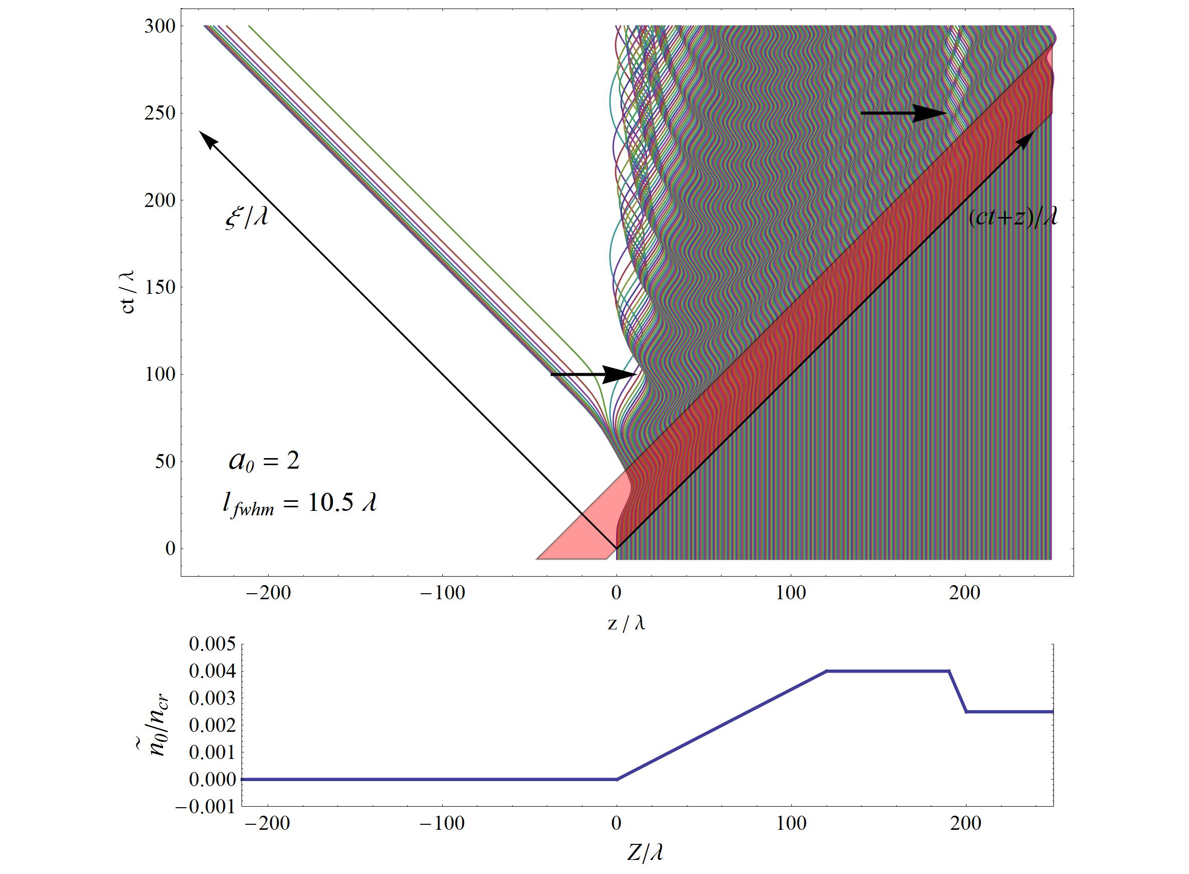
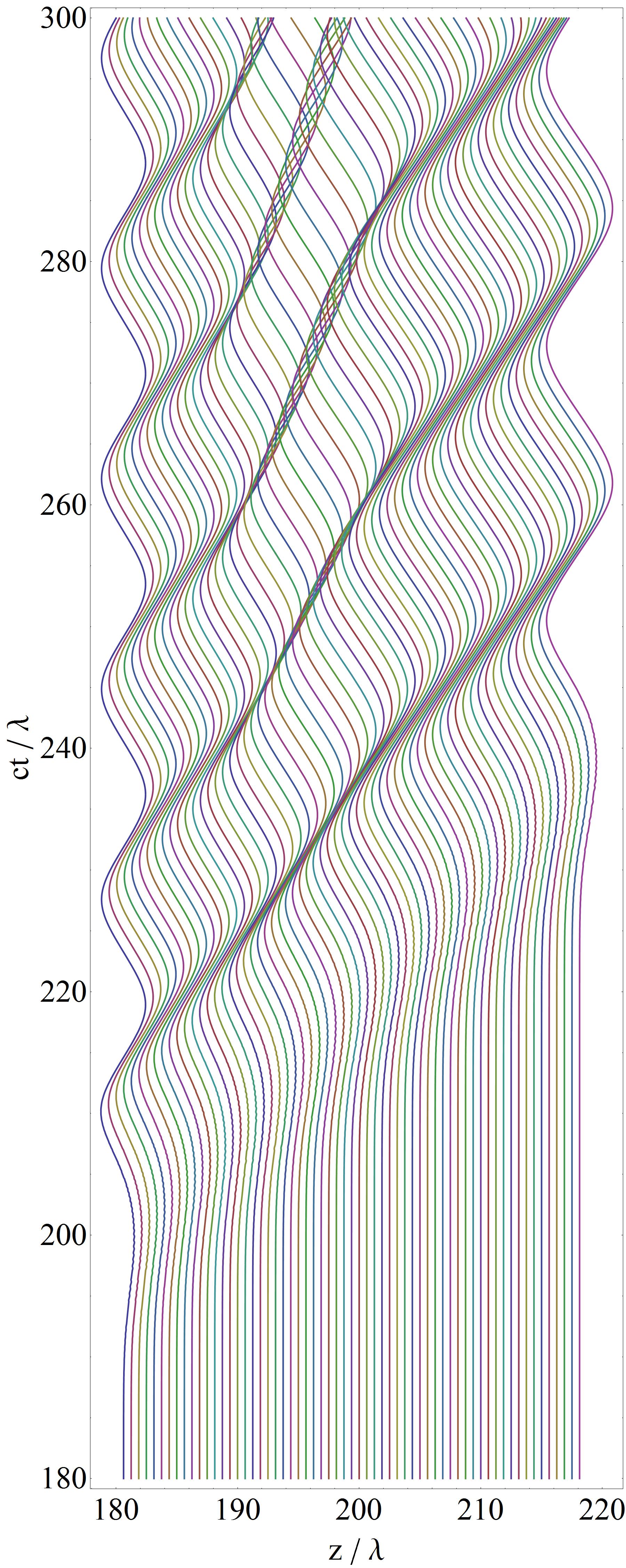
Figure 2: The electron worldlines (WL) induced by the pulse on an initial density $\widetilde{n_{0}}(Z)$ as in section III.B of Ref. BraEtAl08 : WL of $Z\!\sim\!0$ electrons stray left away, WL of other up-ramp electrons first intersect after about $5/4$ oscillations (left arrow), WL of down-ramp electrons first intersect after about $7/4$ oscillations (right arrow; see also the higher resolution plot at the right), consistently with the results obtained in BraEtAl08 by a 2D PIC simulation with a gaussian $\chi\!_{{\scriptscriptstyle R}}(\rho)$ with FWHM equal to $20\lambda$. The support of $\mbox{\boldmath$\epsilon$}^{\scriptscriptstyle\perp}(ct\!-\!z)$ is pink (we have considered $\mbox{\boldmath$\epsilon$}^{\scriptscriptstyle\perp}(\xi)\!=\!0$ outside $0\!<\!\xi\!<\!40\lambda$).

Summarizing, for  $t\!\leq\!t_{c}(z_{s})$  no collisions occur, the maps $z_{e}(t,\cdot)\!:Z\!\mapsto\!z$ are invertible, and the hydrodynamic description is justified. For $t\!>\!t_{c}$ collisions can occur only near the density inhomogeneities; the associated perturbations cannot reach the part of the PW just behind the pulse, as this travels with phase velocity $c$. On the other side, the $Z\!\simeq\!0$ electrons go far backwards before coming back, so are also not affected for long $t$.

Finally, approximating ${\bf A}\!^{\scriptscriptstyle\perp}(t,z)\!\simeq\!{\bm{\alpha}}^{\scriptscriptstyle\perp}(ct\!-\!z)$ is acceptable as long as the so determined motion makes  $|\mbox{rhs}(\ref{inteq1})|\!\ll\!|{\bm{\alpha}}^{\scriptscriptstyle\perp}|$; in the region of interest here this is the case. Otherwise replacing ${\bf A}\!^{\scriptscriptstyle\perp}\mapsto{\bm{\alpha}}^{\scriptscriptstyle\perp}(\xi)$ into rhs(15) determines the first correction to ${\bf A}\!^{\scriptscriptstyle\perp}$; replacing the corrected ${\bf A}\!^{\scriptscriptstyle\perp}$ into (11) and the new $\hat{\bf u}^{\scriptscriptstyle\perp}_{e}$ into (16-17) one can determine the motion with more accuracy; and so on.

III Finite $R$ and discussion

By causality, if two solutions of the dynamic equations coincide in a spacetime region ${\cal D}$, then they coincide also in the future Cauchy development $D^{+}({\cal D})$ (the set of all points $x$ for which every past-directed causal line through $x$ intersects ${\cal D}$). Hence, knowing one solution determines also the other within $D^{+}({\cal D})$. Here all the dynamical variables are exactly known at $t\!=\!0$, and also for $0\leq\!ct\!\leq\!z$ (there the plasma is still at rest and ${\bf E},{\bf B}$ zero). We adopt: i) as ${\cal D}$ the surface ${\cal D}^{0}_{{\scriptscriptstyle R}}$ of equations $\rho\!<\!R$ and either $\!t\!=\!0$, $z\!<\!0$, or $0\leq\!ct\!\leq\!z$; ii) as the known solution the plane one of section II; iii) as the unknown solution the “real” one induced by (2). Hence, at all $t$ all dynamical variables, in particular $n_{e}$ (see fig. 3), are strictly the same as in section II, within the causal cone  ${\cal C}_{t}\!\equiv\!\{(\rho^{\prime}\!,\varphi^{\prime}\!,z^{\prime})\>\>|\>\>0\!\leq\!\rho^{\prime}\!+\!ct\!-\!z^{\prime}\!\leq\!R\}$  (in cylindrical coordinates) trailing the pulse, and approximately the same, in a neighbourhood of it. Hence, for small $t$ there is a “hole” $h_{t}$ in the electron distribution including at least ${\cal C}_{t}\cap L_{t}$, while for larger $t$ the PW behind the pulse is the same inside ${\cal C}_{t}$. If $R$ is ‘large’, wave-breaking around the vacuum-bulk interface takes place also within ${\cal C}_{t}$. Whereas for smaller $R$ fulfilling

$$R\!\gg\!\Delta{\bf x}^{\scriptscriptstyle\perp}_{e},\quad t_{e}\!-\!\bar{t}\sim\frac{R}{c},\quad r\equiv R-\frac{\zeta(t_{e}\!-\!l/c)}{2(t_{e}\!-\!\bar{t})}>0$$ (35)

($\bar{t},t_{e}$ are the times of maximal penetration and expulsion of the $Z\!=\!0$ electrons) the $0\!\leq\!Z\!\leq\!Z_{b}$, $\rho\!\leq\!r\!\leq\!R$ electrons exit the bulk shortly after $C_{t}$ has completely entered it. Conditions (35) respectively ensure: that these electrons move approximately as in section II until their expulsion; that they are expelled before lateral electrons (LE), which are initially located outside the surface $\rho\!=\!R$ and are attracted towards the $\vec{z}$-axis, obstruct them the way out, colliding with each other. The expelled electrons are decelerated by the electric force generated by the net positive charge located at their right within $\rho\!<\!r$, which decreases as $1/z_{e}^{2}$ as $z_{e}\!\to\!-\infty$; this allows the backward escape of a bunch of electrons with high energy ($1\!\div\!5$MeV for a gaussian pulse of energy ${\cal E}\!=\!5$J, $l_{fwhm}\!\simeq\!7.5\mu$m, $\lambda\!\simeq\!0.8\mu$m, spot size $R\!=\!4\!\div\!16\mu$m on a helium jet target), well collimated ($u^{{\scriptscriptstyle\perp}}_{f}\!\simeq\!0$) if $\mbox{\boldmath$\epsilon$}^{\scriptscriptstyle\perp}$ is slowly modulated (slingshot effect). For more details see FioDeN16 .

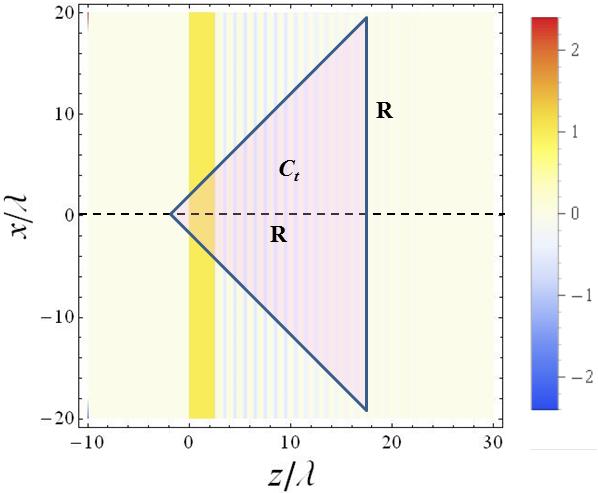
Figure 3: Normalized total charge density $1\!-\!n_{e}/n_{0}$ at $ct=19\lambda$ (conditions as in fig. 1). The electron density ‘hole’ includes the intersection of the ion layer $L_{t}$ (yellow) and causal cone $C_{t}$ (pink) behind the pulse.

If $R$ is even smaller the LE attracted towards the $z$-axis $\vec{z}$ collide closing part of $L_{t}$ into a (possibly temporary) electron cavity (where $n_{e}\!=\!0$) RosBreKat91 ; PukMey2002 before any electrons are expelled backwards. If $R\!\lesssim\!\Delta{\bf x}^{\scriptscriptstyle\perp}_{e{\scriptscriptstyle M}}\!\!\equiv$the maximal transverse oscillations (22), the solution of section II is unreliable even for the ${\bf X}\!=\!(0,0,Z)$ electrons.

We can make the results more explicit if $\mbox{\boldmath$\epsilon$}^{\scriptscriptstyle\perp}$ in (2) is a monochromatic wave modulated by some $\epsilon(\xi)\geq 0$,

$$\mbox{\boldmath$\epsilon$}^{{\scriptscriptstyle\perp}}\!=\!\epsilon\mbox{\boldmath$\epsilon$}_{o}^{{\scriptscriptstyle\perp}},\quad\mbox{\boldmath$\epsilon$}_{o}^{{\scriptscriptstyle\perp}}\!(\xi)\!=\!{\bf i}a_{1}\cos(k\xi\!+\!\varphi_{1})+{\bf j}a_{2}\sin(k\xi\!+\!\varphi_{2}),$$ (36)

with support $[0,l]$ ($a_{1}^{2}\!+\!a_{2}^{2}\!=\!1$). If $f(\xi)$ is a regular function vanishing $\xi\!=\!-\infty$ integration by parts gives

$$\int^{\xi}_{-\infty}\!\!\!\!\!\!d\eta\>f(\eta)e^{ik\eta}=-\frac{i}{k}f(\xi)e^{ik\xi}+O\!\left(\frac{1}{k^{2}}\right);$$ (37)

(the remainder $O(1/k^{2})$ is ‘small’ if $|f^{\prime}|\!\ll\!|kf|$, see Appendix 5.4 of Fio17 ). If $\mbox{\boldmath$\epsilon$}^{\scriptscriptstyle\perp}$ is slowly modulated (i.e. $|\epsilon^{\prime}|\!\ll\!|k\epsilon|$ on $[0,l]$) then  ${\bm{\alpha}}^{\scriptscriptstyle\perp}(\xi)\!\simeq\!\epsilon(\xi)\,\mbox{\boldmath$\epsilon$}^{\scriptscriptstyle\perp}_{o}(\xi\!+\!\pi/2k)$;  hence ${\bm{\alpha}}^{\scriptscriptstyle\perp}(\xi),{\bf u}^{\scriptscriptstyle\perp}(\xi)\!\simeq\!0$ if $\xi\!>\!l$. Since $|f^{\prime}|\!\ll\!|kf|$ holds also for $f\!=\!\hat{s}_{e},\partial\hat{z}_{e}/\partial Z$, (22) yields  $\Delta{\bf x}^{\scriptscriptstyle\perp}_{e}\!\simeq\!-e\mbox{\boldmath$\epsilon$}^{\scriptscriptstyle\perp}/k^{2}mc^{2}\hat{s}_{e}$, and using (24) one can easily estimate $\mbox{rhs}(\ref{inteq1})$, so as to check the condition $R\lesssim|\Delta{\bf x}^{\scriptscriptstyle\perp}_{e{\scriptscriptstyle M}}|$ and the approximation ${\bf A}\!^{\scriptscriptstyle\perp}\!\simeq\!{\bm{\alpha}}^{\scriptscriptstyle\perp}$.

References

(1) T. Tajima, J. M. Dawson, Phys. Rev. Lett. 43 (1979), 267.
(2)
A. I. Akhiezer, R. V. Polovin, Sov. Phys. JETP 3, 696 (1956).
(3)
S. V. Bulanov, V. I. Kirsanov, A. S. Sakharov, JETP Lett. 50, 198 (1989).
(4) J. D. Dawson,
Phys. Rev. 113 (1959), 383.
(5)
S. Bulanov, N. Naumova, F. Pegoraro, J. Sakai, Phys. Rev. E 58, R5257 (1998).
(6)
A. V. Brantov, et al., Phys. Plasmas 15, 073111 (2008).;
(7)
F. Y. Li, et al., Phys. Rev. Lett. 110, 135002 (2013).
(8) G. Fiore, R. Fedele, U. de Angelis,
Phys. Plasmas 21 (2014), 113105.
(9)
G. Fiore, S. De Nicola,
Phys Rev. Acc. Beams 19 (2016), 071302;
Nucl. Instr. Meth. Phys. Res. A829 (2016), 104-108.
(10) G. Fiore,
On the impact of short laser pulses on cold diluted plasmas, in preparation.
(11) G. Fiore,
J. Phys. A: Math. Theor. 47 (2014), 225501.
(12) G. Fiore,
J. Phys. A: Math. Theor. 51 (2018), 085203.
(13) G. Fiore,
Acta Appl. Math. 132 (2014), 261;
Ricerche Mat. 65 (2016), 491-503;
EPJ Web of Conferences 167, 04004 (2018).
(14)
J. Rosenzweig, B. Breizman, T. Katsouleas, J. Su,
Phys. Rev. A44 (1991), R6189.
(15)
A. Pukhov, J. Meyer-ter-Vehn,
Appl. Phys. B74 (2002), 355.