Deep Models of Interactions Across Sets

Abstract

We use deep learning to model interactions across two or more sets of objects, such as user–movie ratings, protein–drug bindings, or ternary user-item-tag interactions. The canonical representation of such interactions is a matrix (or a higher-dimensional tensor) with an exchangeability property: the encoding’s meaning is not changed by permuting rows or columns. We argue that models should hence be Permutation Equivariant (PE): constrained to make the same predictions across such permutations. We present a parameter-sharing scheme and prove that it could not be made any more expressive without violating PE. This scheme yields three benefits. First, we demonstrate state-of-the-art performance on multiple matrix completion benchmarks. Second, our models require a number of parameters independent of the numbers of objects, and thus scale well to large datasets. Third, models can be queried about new objects that were not available at training time, but for which interactions have since been observed. In experiments, our models achieved surprisingly good generalization performance on this matrix extrapolation task, both within domains (e.g., new users and new movies drawn from the same distribution used for training) and even across domains (e.g., predicting music ratings after training on movies).

1 Introduction

Suppose we are given a set of users $\mathbb{N}=\{1,\ldots,N\}$, a set of movies $\mathbb{M}=\{1,\ldots,M\}$, and their interaction in the form of tuples $\mathbb{X}=\langle n,m,x\rangle$ with $n\in\mathbb{N}$, $m\in\mathbb{M}$ and $x\in\mathds{R}$. Our goal is to learn a function that models the interaction between users and movies, i.e., mapping from $N\times M$ to $\mathds{R}$. The canonical representation of such a function is a matrix ${X}\in\mathds{R}^{N\times M}$; of course, we want ${X}_{n,m}=x$ for each $\langle n,m,x\rangle\in\mathbb{X}$. Learning our function corresponds to matrix completion: using patterns in $\mathbb{X}$ to predict values for the remaining elements of ${X}$. $X$ is what we will call an exchangeable matrix: any row- and column-wise permutation of $X$ represents the same set of ratings and hence the same matrix completion problem.

Exchangeability has a long history in machine learning and statistics. de Finetti’s theorem states that exchangeable sequences are the product of a latent variable model. Extensions of this theorem characterize distributions over other exchangeable structures, from matrices to graphs; see Orbanz & Roy (2015) for a detailed treatment. In machine learning, a variety of frameworks formalize exchangeability in data, from plate notation to statistical relational models (Raedt et al., 2016; Getoor & Taskar, 2007). When dealing with exchangeable arrays (or tensors), a common approach is tensor factorization. In particular, one thread of work leverages tensor decomposition for inference in latent variable models (Anandkumar et al., 2014). However, in addition to having limited expressive power, tensor factorization requires retraining models for each new input.

We call a learning algorithm Permutation Equivariant (PE) if it is constrained to give the same answer across all exchangeable inputs; we argue that PE is an important form of inductive bias in exchangeable domains. However, it is not trivial to achieve; indeed, all existing parametric factorization and matrix/tensor completion methods associate parameters with each row and column, and thus are not PE. How can we enforce this property? One approach is to augment the input with all $M!\times N!$ permutations of rows and columns. However, this is computationally wasteful and becomes infeasible for all but the smallest $N$ and $M$. Instead, we show that a simple parameter-sharing scheme suffices to ensure that a deep model can represent only PE functions. The result is analogous to the idea of a convolution layer: a lower-dimensional effective parameter space that enforces a desired equivariance property. Indeed, parameter-sharing is a generic and efficient approach for achieving equivariance in deep models (Ravanbakhsh et al., 2017).

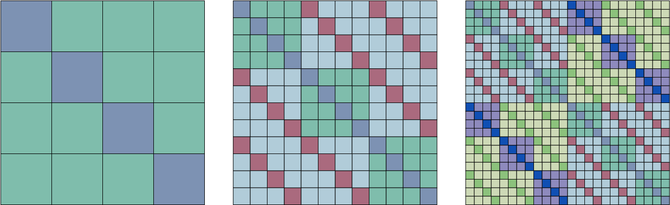
Figure 1: Structure of our parameter matrix for the 1D (left), 2D (centre), and 3D (right) input arrays. The parameter-sharing patterns for the weight matrix of the higher dimensional arrays can be produced via the Kronecker product of the weight matrix for the 1D array (i.e., vector).

When the matrix models the interaction between the members of the same group, one could further constrain permutations to be identical across both rows and columns. An example of such a jointly exchangeable matrix (Orbanz & Roy, 2015), modelling the interaction of the nodes in a graph, is the adjacency matrix deployed by graph convolution. Our approach reduces to graph convolution in the special case of 2D arrays with this additional parameter-sharing constraint, but also applies to arbitrary matrices and higher dimensional arrays.

Finally, we explain connections to some of our own past work. First, we introduced a similar parameter-sharing scheme in the context of behavioral game theory (Hartford et al., 2016): rows and columns represented players’ actions and the exchangeable matrix encoded payoffs. The current work provides a theoretical foundation for these ideas and shows how a similar architecture can be applied much more generally. Second, our model for exchangeable matrices can be seen as a generalization of the deep sets architecture (Zaheer et al., 2017), where a set can be seen as a one-dimensional exchangeable array.

In what follows, we begin by introducing our parameter-sharing approach in Section 2, considering the cases of both dense and sparse matrices. In Section 3.2 we study two architectures for matrix completion that use an exchangeable matrix layer. In particular the factorized autoencoding model provides a powerful alternative to commonly used matrix factorization methods; notably, it does not require retraining to be evaluated on previously unseen data. In Section 4 we present extensive results on benchmark matrix completion datasets. We generalize our approach to higher-dimensional tensors in Section 5.

2 Exchangeable Matrix Layer

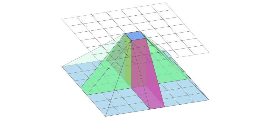
Figure 2: Parameter sharing in an exchangeable matrix layer. The application of different tied parameters to input elements is illustrated using dark blue for $w_{1}$, green for $w_{2}$, red for $w_{3}$, and light blue for $w_{4}$. The same structure (with the same four parameters) repeats across all units of the output layer.

Let ${X}\in\mathds{R}^{N\times M}$ be our “exchangeable” input matrix. We use $\operatorname{vec}({{X}})\in\mathds{R}^{NM}$ to denote its vectorized form and $\operatorname{vec}^{-1}({{x}})$ to denote the inverse of the vectorization that reshapes a vector of length $NM$ into an $N\times M$ matrix—i.e., $\operatorname{vec}^{-1}({\operatorname{vec}({{X}})})={X}$. Consider a fully connected layer ${{Y}}:=\operatorname{vec}^{-1}({\sigma(W\operatorname{vec}({{X}}))})$ where $\sigma$ is an element-wise nonlinear function such as sigmoid, $W\in\mathds{R}^{NM\times NM}$, and ${Y}\in\mathds{R}^{N\times M}$ is the output matrix. Exchangeablity of ${X}$ motivates the following property: suppose we permute the rows and columns ${X}$ using two arbitrary permutation matrices $G^{(N)}\in\{0,1\}^{N\times N}$ and $G^{(M)}\in\{0,1\}^{M\times M}$ to get ${X}^{\prime}:=G^{(N)}{X}G^{(M)}$. Permutation Equivariance (PE) requires the new output matrix ${Y}^{\prime}:=\operatorname{vec}^{-1}({\sigma(W\operatorname{vec}({X^{\prime}}))})$ to experience the same permutation of rows and columns—that is, we require ${Y}^{\prime}=G^{(N)}{Y}G^{(M)}$.

Definition 2.1 (exchangeable matrix layer, simplified).

Given $X\in\mathds{R}^{N\times M}$, a fully connected layer $\sigma(W\operatorname{vec}({X}))$ with $W\in\mathds{R}^{NM\times NM}$ is called an exchangeable matrix layer if, for all permutation matrices $G^{(N)}\in\{0,1\}^{N\times N}$ and $G^{(M)}\in\{0,1\}^{M\times M}$, permutation of the rows and columns results in the same permutations of the output:

$$\operatorname{vec}^{-1}({\sigma(W\operatorname{vec}({G^{(N)}{X}G^{(M)}}))})=$$ (1)

$$\hskip 56.9055ptG^{(N)}\operatorname{vec}^{-1}({\sigma(W\operatorname{vec}({{X}}))})G^{(M)}.$$

This requirement heavily constrains the weight matrix $W$: indeed, its number of effective degrees of freedom cannot even grow with $N$ and $M$. Instead, the resulting layer is forced to have the following, simple form:

$${W}_{(n,m),(n^{\prime},m^{\prime})}:=\begin{cases}w_{1}&n=n^{\prime},m=m^{\prime}\\ w_{2}&n=n^{\prime},m\neq m^{\prime}\\ w_{3}&n\neq n^{\prime},m=m^{\prime}\\ w_{4}&n\neq n^{\prime},m\neq m^{\prime}.\\ \end{cases}$$ (2)

For each output element ${Y}_{n,m}$, we have the following parameters: one connecting it to its counterpart ${X}_{n,m}$; one each connecting it to the inputs of the same row and the inputs of the same column; and one shared by all the other connections. We also include a bias parameter; see Fig. 2 for an illustration of the action of this parameter matrix, and Fig. 1 for a visual illustration of it. Theorem 2.1 formalizes the requirement on our parameter matrix. All proofs are deferred to the appendix.

Theorem 2.1.

Given a strictly monotonic function $\sigma$, a neural layer $\sigma(W\operatorname{vec}({X}))$ is an exchangeable matrix layer iff the elements of the parameter matrix $W$ are tied together such that the resulting fully connected layer simplifies to

$${Y}=\sigma \left(w_{1}^{\prime}{X}+\frac{w_{2}^{\prime}}{N}(\mathbf{1}_{N}\mathbf{1}_{N}^{\mathsf{T}}{X})+\frac{w_{3}^{\prime}}{M}({X}\mathbf{1}_{M}\mathbf{1}_{M}^{\mathsf{T}})\right.$$ (3)

$$+\left.\frac{w_{4}^{\prime}}{NM}(\mathbf{1}_{N}\mathbf{1}_{N}^{\mathsf{T}}{X}\mathbf{1}_{M}\mathbf{1}_{M}^{\mathsf{T}})+w_{5}^{\prime}\mathbf{1}_{N}\mathbf{1}_{M}^{\mathsf{T}}\right)$$

where $\mathbf{1}_{N}=\underbrace{[1,\ldots,1]^{\mathsf{T}}}_{\text{length}N}$ and $w_{1}^{\prime},\ldots,w_{5}^{\prime}\in\mathds{R}$.

This parameter sharing is translated to summing or averaging elements across rows and columns; more generally, PE is preserved by any commutative pooling operation. Moreover, stacking multiple layers with the same equivariance properties preserves equivariance (Ravanbakhsh et al., 2017). This allows us to build deep PE models.

Multiple Input–Output Channels

Equation Eq. 3 describes the layer as though it has single input and output matrices. However, as with convolution, we may have $K$ input and $O$ output channels. We use superscripts ${X}^{\langle k\rangle}$ and ${Y}^{\langle o\rangle}$ to denote such channels. Cross-channel interactions are fully connected—that is, we have five unique parameters $w_{1}^{\langle k,o\rangle},\ldots,w_{4}^{\langle k,o\rangle}$ for each combination of input–output channels; note that the bias parameter $w_{5}$ does not depend on the input. Similar to convolution, the number of channels provides a tuning nob for the expressive power of the model. In this setting, the scalar output ${Y}_{n,m}^{\langle o\rangle}$ is given as

$${Y}^{\langle o\rangle}_{n,m} =\sigma\left(\sum_{k=1}^{K}\bigg{(}w_{1}^{\langle k,o\rangle}{X}_{n,m}^{\langle k\rangle}+\frac{w_{2}^{\langle k,o\rangle}}{N}(\sum_{n^{\prime}}{X}_{n^{\prime},m}^{\langle k\rangle})+\right.$$ (4)

$$\left.\frac{w_{3}^{\langle k,o\rangle}}{M}(\sum_{m^{\prime}}{X}_{n,m^{\prime}}^{\langle k\rangle})+\frac{w_{4}^{\langle k,o\rangle}}{NM}(\sum_{n^{\prime},m^{\prime}}{X}_{n^{\prime},m^{\prime}}^{\langle k\rangle})+w_{5}^{\langle o\rangle}\bigg{)}\right)$$

Input Features for Rows and Columns

In some applications, in addition to the matrix ${X}\in\mathds{R}^{N\times M\times K}$, where $K$ is the number of input channels/features, we may have additional features for rows $R\in\mathds{R}^{N\times K^{\prime}}$ and/or columns $C\in\mathds{R}^{M\times K^{\prime\prime}}$. We can preserve PE by broadcasting these row/column features over the whole matrix and treating them as additional input channels.

Jointly Exchangeable Matrices

For jointly exchangeable matrices, such as adjacency matrix, Equation Eq. 1 is constrained to have $N=M$ and $G^{(N)}=G^{(M)}$. This will in turn constrain the corresponding parameter-sharing so that $w_{2}=w_{3}$ in Equation Eq. 2.

2.1 Sparse Inputs

Real-world arrays are often extremely sparse. Indeed, matrix and tensor completion is only meaningful with missing entries. Fortunately, the equivariance properties of Theorem 2.1 continue to hold when we only consider the nonzero (observed) entries. For sparse matrices, we continue to use the same parameter-sharing scheme across rows and columns, with the only difference being that we limit the model to observed entries. We now make this precise.

Let ${X}\in\mathds{R}^{N\times M\times K}$ be a sparse exchangeable array with $K$ channels, where all the channels for each row-column pair $\langle n,m\rangle$ are either fully observed or completely missing. Let $\mathbb{I}$ identify the set of such non-zero indices. Let $\mathbb{R}_{n}=\{m\mid(n,m)\in\mathbb{I}\}$ be the non-zero entries in the $n^{th}$ row of ${X}$, and let $\mathbb{C}_{m}$ be the non-zero entries of its $m^{th}$ column. For this sparse matrix, the terms in the layer of Eq. 4 are adapted as one would expect:

$$\frac{w_{2}^{\langle k,o\rangle}}{N}\sum_{n^{\prime}}{X}_{n^{\prime},m}^{\langle k\rangle}\quad\rightarrow\quad\frac{w_{2}^{\langle k,o\rangle}}{|\mathbb{C}_{m}|}\sum_{n^{\prime}\in\mathbb{C}_{m}}{X}_{n^{\prime},m}^{\langle k\rangle}$$

$$\frac{w_{3}^{\langle k,o\rangle}}{M}\sum_{m^{\prime}}{X}_{n,m^{\prime}}^{\langle k\rangle}\quad\rightarrow\quad\frac{w_{3}^{\langle k,o\rangle}}{|\mathbb{R}_{n}|}\sum_{m^{\prime}\in\mathbb{R}_{n}}{X}_{n,m^{\prime}}^{\langle k\rangle}$$

$$\frac{w_{4}^{\langle k,o\rangle}}{NM}\sum_{n^{\prime},m^{\prime}}{X}_{n^{\prime},m^{\prime}}^{\langle k\rangle}\quad\rightarrow\quad\frac{w_{4}^{\langle k,o\rangle}}{|\mathbb{I}|}\sum_{(n^{\prime},m^{\prime})\in\mathbb{I}}{X}_{n^{\prime},m^{\prime}}^{\langle k\rangle}$$

3 Matrix Factorization and Completion

Recommender systems are very widely applied, with many modern applications suggesting new items (e.g., movies, friends, restaurants, etc.) to users based on previous ratings of other items. The core underlying problem is naturally posed as a matrix completion task: each row corresponds to a user and each column corresponds to an item; the matrix has a value for each rating given to an item by a given user; the goal is to fill in the missing values of this matrix.

In Section 3.1 we review two types of analysis in dealing with exchangeable matrices. Section 3.2 introduces two architectures: a self-supervised model—a simple composition of exchangeable matrix layers—that is trained to produce randomly removed entries of the observed matrix during the training; and a factorized model that uses an auto-encoding nonlinear factorization scheme. While there are innumerable methods for (nonlinear) matrix factorization and completion, both of these models are the first to generalize to inductive settings while achieving competitive performance in transductive settings. Section 3.3 introduces two subsampling techniques for large sparse matrices followed by a literature review in Section 3.4.

3.1 Inductive and Transductive Analysis

In matrix completion, during training we are given a sparse input matrix ${X}_{\text{tr}}$ with observed entries $\mathbb{I}_{\text{tr}}=\{(n,m)\}$. At test time, we are given ${X}_{\text{ts}}$ with observed entries $\mathbb{I}_{\text{ts}}=\{(n^{\prime},m^{\prime})\}$, and we are interested in predicting (some of) the missing entries of ${X}_{\text{ts}}$, expressed through $\mathbb{I}^{\prime}_{\text{ts}}$. In the transductive or matrix interpolation setting, $\mathbb{I}_{\text{tr}}$ and $\mathbb{I}_{\text{ts}}$ have overlapping rows and/or columns—that is, at least one of the following is true: $\{m\mid(n,m)\in\mathbb{I}\}\cap\{m^{\prime}\mid(n^{\prime},m^{\prime})\in\mathbb{I}^{\prime}\}\neq\emptyset$ or $\{n\mid(n,m)\in\mathbb{I}\}\cap\{n^{\prime}\mid(n^{\prime},m^{\prime})\in\mathbb{I}^{\prime}\}\neq\emptyset$. In fact, often ${X}_{\text{tr}}$ and ${X}_{\text{ts}}$ are identical. Conversely, in the inductive or matrix extrapolation setting, we are interested in making predictions about completely unseen entries: the training and test row/column indices are completely disjoint. We will even consider cases where ${X}_{\text{tr}}$ and ${X}_{\text{ts}}$ are completely different datasets—e.g., movie-rating vs music-rating. The same distinction applies in matrix factorization. Training a model to factorize a particular given matrix is transductive, while factorizing unseen matrices after training is inductive.

3.2 Architectures

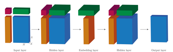
Figure 3: Factorized exchangeable autoencoder. The encoder maps from the input tensor to an embedding layer of row / column factors via one or more hidden layers. The decoder attempts to reconstruct the input using the factors via one or more hidden layers.

Self-supervised Exchangeable Model

When the task is matrix completion, a simple deep yet PE model is a composition of exchangeable matrix layers. That is the function $f_{ss}:\mathds{R}^{N\times M\times K}\to\mathds{R}^{N\times M\times K}$ is simply a composition of exchangeable matrix layers. Given the matrix ${X}$ with observed entries $\mathbb{I}$, we divide $\mathbb{I}=\mathbb{I}_{\text{in}}\cup\mathbb{I}_{\text{pr}}$ into disjoint input and prediction entries. We then train $f_{ss}({X}_{\text{in}})$ to predict the prediction entries ${X}_{\text{pr}}$.

Factorized Exchangeable Autoencoder (FEA)

Our factorized autoencoder is composed of an encoder and a decoder. The encoder $f_{\text{enc}}:\mathds{R}^{N\times M\times K}\to\mathds{R}^{K_{N}\times N}\times\mathds{R}^{K_{M}\times M}$ maps the (sparse) input matrix ${X}\in\mathds{R}^{N\times M\times K}$ to a row-factor ${Z}_{N}\in\mathds{R}^{K_{N}\times N}$ and a column-factor ${Z}_{M}\in\mathds{R}^{K_{M}\times M}$. To do so, the encoder uses a composition of exchangeable matrix layers. The output of the final layer ${Y}^{l}\in\mathds{R}^{N\times M\times K^{l}}$ is pooled across rows and columns (and optionally passed through a feed-forward layer) to produce latent factors ${Z}_{N}$ and ${Z}_{M}$. The decoder $g_{\text{dec}}:\mathds{R}^{K_{N}\times N}\times\mathds{R}^{K_{M}\times M}\to\mathds{R}^{N\times M\times K}$ also uses a composition of exchangeable matrix layers, and reconstructs the input matrix ${X}$ from the factors. The optimization objective is to minimize reconstruction error $\ell({X},g_{\text{dec}}(f_{enc}({X})))$; similar to classical auto-encoders.

This procedure is also analogous to classical matrix factorization, with an an important distinction that once trained, we can readily factorize the unseen matrices without performing any optimization. Note that the same architecture trivially extends to tensor-factorization, where we use an exchangeable tensor layer (see Section 5).

Channel Dropout

Both the factorized autoencoder and self-supervised exchangeable model are flexible enough to make regularization important for good generalization performance. Dropout (Srivastava et al., 2014) can be extended to apply to exchangeable matrix layers by noticing that each channel in an exchangeable matrix layer is analogous to a single unit in a standard feed-forward network. We therefore randomly drop out whole channels during training (as opposed to dropping out individual elements). This procedure is equivalent to the SpatialDropout technique used in convolutional networks (Tompson et al., 2015).

3.3 Subsampling in Large Matrices

A key practical challenge arising from our approach is that our models are designed to take the whole data matrix ${X}$ as input and will make different (and typically worse) predictions if given only a subset of the data matrix. As datasets grow, the model and input data become too large to fit within fixed-size GPU memory. This is problematic both during training and at evaluation time because our models rely on aggregating shared representations across data points to make their predictions. To address this, we explore two subsampling procedures.

Uniform sampling

The simplest approach is to sample sub-matrices of ${X}$ by uniformly sampling from its (typically sparse) elements. This has the advantage that each submatrix is an unbiased sample of the full matrix and that the procedure is computationally cheap, but has the potential to limit the performance of the model because the relationships between the elements of ${X}$ are sparsified.

Conditional sampling

Rather than sparsifying interactions between all set members, we can pick a subset of rows and columns and maintain all their interactions; see Figure 4. This procedure is unbiased as long as each element $(n,m)\in\mathbb{I}$ has the same probability of being sampled. To achieve this, we first sample a subset of rows $\mathbb{N}^{\prime}\subseteq\mathbb{N}=\{1,\ldots,N\}$ from the marginal $P(n):=\frac{|\mathbb{R}_{n}|}{|\mathbb{I}|}$, followed by subsampling of colums using the marginal distribution over the columns, within the selected rows: $P(m\mid\mathbb{N}^{\prime})=\frac{|\{(m,n)\in\mathbb{I}\mid n\in\mathbb{N}^{\prime}\}|}{\{(m^{\prime},n)\in\mathbb{I}\mid n\in\mathbb{N}^{\prime}\}|}$. This gives us a set of columns $\mathbb{M}^{\prime}\subseteq\mathbb{M}$. We consider any observation within $\mathbb{N}^{\prime}\times\mathbb{M}^{\prime}$ as our subsample: $\mathbb{I}_{\text{sample}}:=\{(n,m)\in\mathbb{I}\mid n\in\mathbb{N}^{\prime},m\in\mathbb{M}^{\prime}\}$. This sampling procedure is more expensive than uniform sampling, as we have to calculate conditional marginal distributions for each set of samples.

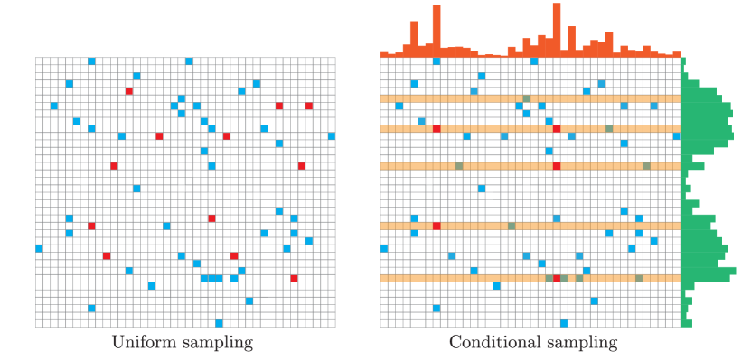
Figure 4: Uniform sampling (left) selects samples (red) uniformly from the non-zero indices of the the matrix ${X}$ while conditional sampling (right) first samples a set of rows (shown in orange) from the row marginal distribution (green) and then selects sample from the resulting column conditional distribution.

Sampling at test time

At training time all we must ensure is that we sample in an unbiased way; however, at test time we need to ensure that the test indices $\mathbb{I}_{\text{ts}}$ of large test matrix ${X}_{\text{ts}}$ are all sampled. Fortunately, according to the coupon collectors’ lemma, in expectation we only need to repeat random sampling of indices $\log(|\mathbb{I}_{\text{ts}}|)$ times more ($\approx 10\times$ in practice) than an ideal partitioning of $\mathbb{I}_{\text{ts}}$, in order to cover all the relevant indices.

3.4 Related Literature

The literature in matrix factorization and completion is vast. The classical approach to solving the matrix completion problem is to find some low rank (or sparse) approximation that minimizes a reconstruction loss for the observed ratings (see e.g., Candès & Recht, 2009; Koren et al., 2009; Mnih & Salakhutdinov, 2008). Because these procedures learn embeddings for each user and item to make predictions, they are transductive, meaning they can only make predictions about users and items observed during training. To our knowledge this is also true for all recent deep factorization and other collaborative filtering techniques (e.g.,  Salakhutdinov et al., 2007; Deng et al., ; Sedhain et al., 2015; Wang et al., 2015; Li et al., 2015; Zheng et al., 2016; Dziugaite & Roy, 2015). An exception is a recent work by Yang et al. (2016) that extends factorization-style approaches to the inductive setting (where predictions can be made on unseen users and items). However their method relies on additional side information to represent users and items. By contrast, our approach is able to make inductive completions on rating matrices that may differ from that which was observed during training without using any side information (though our approach can easily incorporate side information).

Matrix completion may also be posed as predicting edge weights in bipartite graphs (Berg et al., 2017; Monti et al., 2017). This approach builds on recent work applying convolutional neural networks to graph-structured data (Scarselli et al., 2009; Bruna et al., 2014; Duvenaud et al., 2015; Defferrard et al., 2016; Kipf & Welling, 2016; Hamilton et al., 2017). As we saw, parameter sharing in graph convolution is closely related to parameter sharing in exchangeable matrices, and indeed it is a special case where $w_{2}=w_{3}$ in Equation Eq. 2.

4 Empirical Results

For reproducibility we have released Tensorflow and Pytorch implementations of our model. Details on the training and architectures appear in the appendix. Section 4.1 reports experimental results in the standard transductive (matrix interpolation) setting. However, more interesting results are reported in Section 4.2, where we test a trained deep model on a completely different dataset. Finally Section 4.3 compares the model’s performance when using different sampling procedures. The datasets used in our experiments are summarized in Table 1.

Dataset	Users	Items	Ratings	Sparsity
MovieLens 100K	943	1682	100,000	6.30%
MovieLens 1M	6040	3706	1,000,209	4.47%
Flixster	3000	3000	26173	0.291%
Douban	3000	3000	136891	1.521%
Yahoo Music	3000	3000	5335	0.059%
Netflix	480,189	17,770	100,480,507	1.178%

Table 1: Number of users, items and ratings for the data sets used in our experiments. MovieLens data sets are standard (Harper & Konstan, 2015), as is Netflix, while for Flixster, Douban and Yahoo Music we used the $3000\times 3000$ submatrix presented by (Monti et al., 2017) for comparison purposes.

4.1 Transductive Setting (Matrix Interpolation)

Here, we demonstrate that exploiting the PE structure of the exchangeable matrices allows us to achieve results competitive with state-of-the-art, while maintaining a constant number of parameters. Note that the number of parameters in all the competing methods grow with $N$ and/or $M$.

In Table 2 we report that the self-supervised exchangeable model is able to achieve state of the art performance on MovieLens-100K dataset. For MovieLens-1M dataset, we cannot fit the whole dataset into the GPU memory for training and therefore use conditional subsampling; also see Section 4.3. Our results on this dataset are summarized in table Table 3. On this larger dataset both models gave comparatively weaker performance than what we observed on the smaller ML-100k dataset and in the extrapolation results. We suspect this is largely due to memory constraints: there is a trade-off between the size of the model (in terms of number of layers and units per layer) and the batch size one can train. We found that both larger batches and deeper models tended to offer better performance, but on these larger datasets it is not currently possible to have both. The results for the factorized exchangeable autoencoder architecture are similar and reported in the same table.

Model	ML-100K
MC (Candès & Recht, 2009)	0.973
GMC (Kalofolias et al., 2014)	0.996
GRALS (Rao et al., 2015)	0.945
sRGCNN (Monti et al., 2017)	0.929
Factorized EAE (ours)	0.920
GC-MC (Berg et al., 2017)	0.910
Self-Supervised Model (ours)	0.910

Table 2: Comparison of RMSE scores for the MovieLens-100k dataset, based on the canonical 80/20 training/test split. Baseline numbers are taken from (Berg et al., 2017).

Model	ML-1M
PMF (Mnih & Salakhutdinov, 2008)	0.883
Self-Supervised Model (ours)	0.863
Factorized EAE (ours)	0.860
I-RBM (Salakhutdinov et al., 2007)	0.854
BiasMF (Koren et al., 2009)	0.845
NNMF (Dziugaite & Roy, 2015)	0.843
LLORMA-Local (Lee et al., 2013)	0.833
GC-MC (Berg et al., 2017)	0.832
I-AUTOREC (Sedhain et al., 2015)	0.831
CF-NADE (Zheng et al., 2016)	0.829

Table 3: Comparison of RMSE scores for the MovieLens-1M dataset on random 90/10 training/test split. Baseline numbers are taken from (Berg et al., 2017).

4.2 Inductive Setting (Matrix Extrapolation)

Because our model does not rely on any per-user or per-movie parameters, it should be able to generalize to new users and movies that were not present during training. We tested this by training an exchangeable factorized autoencoder on the MovieLens-100k dataset and then evaluating it on a subsample of data from the MovieLens-1M dataset. At test time, the model was shown a portion of the new ratings and then made to make predictions on the remaining ratings.

Figure 5 summarizes the results where we vary the amount of data shown to the model from 5% of the new ratings up to 95% and compare against K-nearest neighbours approaches. Our model significantly outperforms the baselines in this task and performance degrades gracefully as we reduce the amount of data observed.

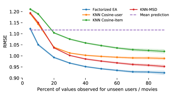
Figure 5: Evaluation of our model’s ability to generalize. We trained on ML-100k and evaluated on a subset of the ML-1M data. At evaluation time, $p\%$ of the ML-1M data was treated as observed and the model was required to complete the remaining $(1-p)\%$ ($p$ varied from $5\%$ to $95\%$). The model outperforms nearest-neighbour approaches for all values of $p$ and degrades gracefully to the baseline of predicting the mean in the small data case.

Extrapolation to new datasets

Perhaps most surprisingly, we were able to achieve competitive results when training and testing on completely disjoint datasets. For this experiment we stress-tested our model’s inductive ability by testing how it generalizes to new datasets without retraining. We used a Factorized Exchangeable Autoencoder that was trained to make predictions on the MovieLens-100k dataset and tasked it with making predictions on the Flixster, Douban and YahooMusic datasets. We then evaluated its performance against models trained for each of these individual datasets. All the datasets involve rating prediction tasks, so they share some similar semantics with MovieLens, but they have different user bases and (in the case of YahooMusic) deal with music not movie ratings, so we may expect some change in the rating distributions and user-item interactions. Furthermore, the Flixster ratings are in 0.5 point increments from $1-5$ and YahooMusic allows ratings from $1-100$, while Douban and MovieLens ratings are on $1-5$ scale. To account for the different rating scales, we simply binned the inputs to our model to a $1-5$ range and, where applicable, linearly rescaled the output before comparing it to the true rating. Despite all of this, Table 4 shows that our model achieves very competitive results with models that were trained for the task.

For comparison, we also include the performance of a Factorized EAE trained on the respective datasets. This improves performance of our model over previous state of the art results on the Flixster and YahooMusic datasets and gives very similar performance to Berg et al. (2017)’s GC-MC model on the Douban dataset. Interestingly, we see the largest performance gains over existing approaches on the datasets in which ratings are sparse (see Table 1).

4.3 Comparison of sampling procedures

We evaluated the effect of subsampling the input matrix ${X}$ on performance, for the MovieLens-100k dataset. The results are summarized in Figure 6. The two key findings are: I) even with large batch sizes of 20 000 examples, performance for both sampling methods is diminished compared to the full batch case. We suspect that our models’ weaker results on the larger ML-1M dataset may be partially attributed to the need to subsample. II) the conditional sampling method was able to recover some of the diminished performance. We believe it is likely that more sophisticated sampling schemes that explicitly take into account the dependence between hidden nodes will lead to better performance but we leave that to future work.

Model	Flixster	Douban	YahooMusic	Netflix
GRALS (Rao et al., 2015)	1.313	0.833	38.0	-
sRGCNN (Monti et al., 2017)	1.179	0.801	22.4	-
GC-MC (Berg et al., 2017)	0.941	0.734	20.5	-
Factorize EAE (ours)	0.908	0.738	20.0	-
Factorize EAE (trained on ML100k)	0.987	0.766	23.3	0.918
Netflix Baseline	-	-	-	0.951
PMF (Mnih & Salakhutdinov, 2008)	-	-	-	0.897
LLORMA-Local (Lee et al., 2013)	-	-	-	0.834
I-AUTOREC (Sedhain et al., 2015)	-	-	-	0.823
CF-NADE (Zheng et al., 2016)	-	-	-	0.803

Table 4: Evaluation of our model’s ability to generalize across datasets. We trained a factorized model on ML100k and then evaluated it on four new datasets. Results for the smaller datasets are taken from (Berg et al., 2017). Netflix Baseline shows state of the art prior to the Netflix Challenge.

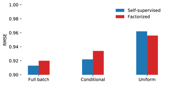
Figure 6: Performance difference between sampling methods on the ML-100k. The two sampling methods use minibatches of size 20 000, while the full batch method used all 75 000 training examples. Note that the y-axis does not begin at 0.

5 Extention to Tensors

In this section we generalize the exchangeable matrix layer to higher-dimensional arrays (tensors) and formalize its optimal qualities. Suppose ${X}\in\mathds{R}^{N_{1}\times...\times N_{D}}$ is our $D$-dimensional data tensor, and $\operatorname{vec}({{X}})$ its vectorized form. We index $\operatorname{vec}({{X}})$ by tuples $(n_{1},n_{2},...,n_{D})$, corresponding to the original dimensions of ${X}$. The precise method of vectorization is irrelevant, provided it is used consistently. Let $\mathscr{N}=\prod_{i}N_{i}$ and let $\underline{n}=(n_{i},n_{-i})$ be an element of ${N_{1}\times...\times N_{D}}$ such that $n_{i}$ is the value of the $i$-th entry of $\underline{n}$, and $n_{-i}$ the values of the remaining entries (where it is understood that the ordering of the elements of $\underline{n}$ is unchanged). We seek a layer that is equivariant only to certain, meaningful, permutations of $\operatorname{vec}({{X}})$. This motivates our definition of an exchangeable tensor layer in a manner that is completely analogous to Definition 2.1 for matrices.

For any positive integer $N$, let $\mathcal{S}^{(N)}$ denote the symmetric group of all permutations of $N$ objects. Then $\mathcal{S}^{(N_{1})}\times...\times\mathcal{S}^{(N_{D})}$ refers to the product group of all permutations of $N_{1}$ through $N_{D}$ objects, while $\mathcal{S}^{(\mathscr{N})}$ refers to the group of all permutations of $\mathscr{N}=\prod_{i}N_{i}$ objects. So $\mathcal{S}^{(N_{1})}\times...\times\mathcal{S}^{(N_{D})}$ is a proper subgroup of $\mathcal{S}^{(\mathscr{N})}$ having $\prod_{i}(N_{i}!)$ members, compared to $(\prod_{i}N_{i})!$ members in $\mathcal{S}^{(\mathscr{N})}$. We want a layer that is equivariant to only those permutations in $\mathcal{S}^{(N_{1})}\times...\times\mathcal{S}^{(N_{D})}$, but not to any other member of $\mathcal{S}^{(\mathscr{N})}$.

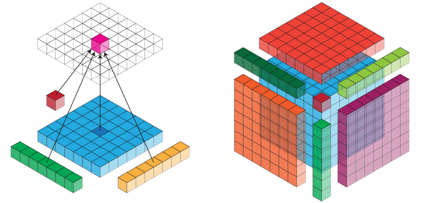
Figure 7: Pooling structure implied by the tied weights for matrices (left) and 3D tensors (right). The pink cube highlights one element of the output. It is calculated as a function of the corresponding element from the input (dark blue), pooled aggregations over the rows and columns of the input (green and yellow), and pooled aggregation over the whole input matrix (red). In the tensor case (right), we pool over all sub-tensors (orange and purple sub-matrices, green sub-vectors and red scalar). For clarity, the output connections are not shown in the tensor case.

Definition 5.1 (exchangeable tensor layer).

Let $\mathcal{g}^{(\mathscr{N})}\in\mathcal{S}^{(N_{1})}\times\mathcal{S}^{(N_{2})}\times...\times\mathcal{S}^{(N_{D})}$ and ${G}^{(\mathscr{N})}$ be the corresponding permutation matrix. Then the neural layer $\operatorname{vec}^{-1}({\sigma({W}\operatorname{vec}({{X}}))})$ with ${X}\in\mathds{R}^{N_{1}\times\ldots\times N_{D}}$ and ${W}\in\mathds{R}^{\mathscr{N}\times\mathscr{N}}$ is an exchangeable tensor layer if permuting the elements of the input along any set of axes results in the same permutation of the output tensor:

$$G^{(\mathscr{N})}\sigma(W\operatorname{vec}({X}))=\sigma(WG^{(\mathscr{N})}\operatorname{vec}({X}))\quad\forall{X},$$ (5)

and moreover for any other permutation of the elements ${X}$ (i.e., permutations that are not along axes), there exists an input ${X}$ for which this equality does not hold.

The following theorem asserts that a simple parameter tying scheme achieves the desired permutation equivariance for tensor-structured data.

Theorem 5.1.

The layer ${{Y}}=\operatorname{vec}^{-1}({\sigma({W}\operatorname{vec}({{X}}))})$, where $\sigma$ is any strictly monotonic, element-wise nonlinearity (e.g., sigmoid), is an exchangeable tensor layer iff the parameter matrix ${W}\in\mathds{R}^{\mathscr{N}\times\mathscr{N}}$ is defined as follows.

For each $\mathbb{S}\subseteq[D]=\{1,\ldots,D\}$, define a distinct parameter $w_{\mathbb}{S}\in\mathds{R}$, and tie the entries of ${W}$ as follows

$${W}_{\underline{n},\underline{n}^{\prime}} :=w_{\mathbb}{S}\quad\text{s.t.}\quad n_{i}=n_{i}^{\prime}\iff i\in\mathbb{S}.$$ (6)

That is, the $(\underline{n},\underline{n}^{\prime})$-th element of ${W}$ is uniquely determined by the set of indices at which $n$ and $n^{\prime}$ are equal.

In the special case that ${X}\in\mathds{R}^{N_{1}\times N_{2}}$ is a matrix, this gives the formulation of ${W}$ described in Section 2. Theorem 5.1 says that a layer constructed in this manner is equivariant with respect to only those permutations of $\mathscr{N}$ objects that correspond to permutations of sub-tensors along the $D$ dimensions of the input. The proof is in the Appendix. Equivariance with respect to permutations in $\mathcal{S}^{(N_{1})}\times\mathcal{S}^{(N_{2})}\times...\times\mathcal{S}^{(N_{D})}$) follows as a simple corollary of Theorem 2.1 in (Ravanbakhsh et al., 2017). Non-equivariance with respect to other permutations follows from the following Propositions.

Proposition 5.2.

Let $\mathcal{g}^{(\mathscr{N})}\in\mathcal{S}^{(\mathscr{N})}$ be an “illegal” permutation of elements of the tensor $X$ – that is $\mathcal{g}^{(\mathscr{N})}\not\in\mathcal{S}^{(N_{1})}\times\mathcal{S}^{(N_{2})}\times...\times\mathcal{S}^{(N_{D})}$. Then there exists a dimension $i\in[D]$ such that, for some $n_{i},n_{i}^{\prime},n_{-i},n_{-i}^{\prime}$:

$$\mathcal{g}^{(\mathscr{N})}((n_{i},n_{-i})) =(n_{i}^{\prime},n_{-i}),\quad\text{but}$$

$$\mathcal{g}^{(\mathscr{N})}((n_{i},n_{-i}^{\prime})) \neq(n_{i}^{\prime},n_{-i}^{\prime}).$$

If we consider the sub-tensor of ${X}$ obtained by fixing the value of the $i$-th dimension to $n_{i}$, we expect a “legal” permutation to move this whole subtensor to some $n_{i}^{\prime}$ (it could additionally shuffle the elements within this subtensor.) This Proposition asserts that an “illegal” permutation $\mathcal{g}^{(\mathscr{N})}\not\in\mathcal{S}^{(N_{1})}\times\mathcal{S}^{(N_{2})}\times...\times\mathcal{S}^{(N_{D})}$ is guaranteed to violate this constraint for some dimension/subtensor combination. The next proposition asserts that if we can identify such inconsistency in permutation of sub-tensors then we can identify and entry in ${G}^{(\mathscr{N})}{W}$ that will differ from ${W}{G}^{(\mathscr{N})}$, and therefore for some input tensor $X$, the equivariance property is violated – i.e., $G^{(\mathscr{N})}\sigma(W\operatorname{vec}({X}))\neq\sigma(WG^{(\mathscr{N})}\operatorname{vec}({X}))$.

Proposition 5.3.

Let $\mathcal{g}^{(\mathscr{N})}\in\mathcal{S}^{(\mathscr{N})}$ with ${G}^{(\mathscr{N})}\in\{0,1\}^{\mathscr{N}\times\mathscr{N}}$ the corresponding permutation matrix. Suppose $\mathcal{g}^{(\mathscr{N})}\not\in\mathcal{S}^{(N_{1})}\times\mathcal{S}^{(N_{2})}\times...\times\mathcal{S}^{(N_{D})}$, and let ${W}\in\mathds{R}^{\mathscr{N}\times\mathscr{N}}$ be as defined above. If there exists an $i\in[D]$, and some $n_{i},n_{i}^{\prime},n_{-i},n_{-i}^{\prime}$ such that

$$\mathcal{g}^{(\mathscr{N})}((n_{i},n_{-i})) =(n_{i}^{\prime},n_{-i}),\quad\text{and}$$

$$\mathcal{g}^{(\mathscr{N})}((n_{i},n_{-i}^{\prime})) \neq(n_{i}^{\prime},n_{-i}^{\prime}),$$

then

$$\big{(}{G}^{(\mathscr{N})}{W}\big{)}_{(n_{i}^{\prime},n_{-i}^{\prime}),(n_{i},n_{-i})}\neq\big{(}{W}{G}^{(\mathscr{N})}\big{)}_{(n_{i}^{\prime},n_{-i}^{\prime}),(n_{i},n_{-i})}$$

Proposition 5.3 makes explicit a particular element at which the products ${G}^{(N)}{W}$ and ${W}{G}^{(N)}$ will differ, provided $\mathcal{g}^{(\mathscr{N})}$ is not of the desired form.

Theorem 5.1 shows that this parameter sharing scheme produces a layer that is equvariant to exactly those permutations we desire, and moreover, it is optimal in the sense that any layer having fewer ties in its parameters (i.e., more parameters) would fail to be equivariant.

Conclusion

This paper has considered the problem of predicting relationships between the elements of two or more distinct sets of objects, where the data can also be expressed as an exchangeable matrix or tensor. We introduced a weight tying scheme enabling the application of deep models to this type of data. We proved that our scheme always produces permutation equivariant models and that no increase in model expressiveness is possible without violating this guarantee. Experimentally, we showed that our models achieve state-of-the-art or competitive performance on widely studied matrix completion benchmarks. Notably, our models achieved this performance despite having a number of parameters independent of the size of the matrix to be completed, unlike all other approaches that offer strong performance. Also unlike these other approaches, our models can achieve competitive results for the problem of matrix extrapolation: asking an already-trained model to complete a new matrix involving new objects that were unobserved at training time. Finally, we observed that our methods were surprisingly strong on various transfer learning tasks: extrapolating from MovieLens ratings to Fixter, Douban, and YahooMusic ratings. All of these contained different user populations and different distributions over the objects being rated; indeed, in the YahooMusic dataset, the underlying objects were not even of the same kind as those rated in training data.

Appendix A Notation

• ${X}\in\mathds{R}^{N_{1}\times...\times N_{D}}$, the data tensor

• ${x}\in\mathds{R}^{\prod_{i}N_{i}}$, vectorized ${X}$, also denoted by $\operatorname{vec}({{X}})$.

• $[N]$: the sequence $\{n\}_{n=1,...,N}=(1,2,...N)$

• $[N_{1}\times...\times N_{D}]$, the sequence $\{(n_{1},...,n_{D})\}_{n_{1}\in[N_{1}],...,n_{D}\in[N_{D}]}$ of $D$-dimensional tuples over $N_{1}\times...\times N_{D}$

• $\underline{n}=(n_{i},n_{-i})$, an element of ${N_{1}\times...\times N_{D}}$

• $\mathscr{N}=\prod_{i}N_{i}$

• $\mathcal{S}^{(N)}$, symmetric group of all permutations of $N$ objects

• $\mathcal{G}^{(N)}=\{\mathcal{g}^{(N)}_{i}\}_{i}$, a permutation group of $N$ objects

• $\mathcal{g}^{(N)}_{i}$ or ${G}_{i}^{(N)}$, both can refer to the matrix form of the permutation $\mathcal{g}^{(N)}_{i}\in\mathcal{G}^{(N)}$.

• $\mathcal{g}^{(N)}_{i}(n)$ refers to the result of applying $\mathcal{g}^{(N)}_{i}$ to $n$, for any $n\in[N]$.

• $\sigma$, an arbitrary, element-wise, strictly monotonic, nonlinear function such as sigmoid.

Appendix B Proofs

B.1 Proof of Proposition 5.2

Proof.

Let ${X}\in\mathds{R}^{N_{1}\times...\times N_{D}}$ be the data matrix. We prove the contrapositive by induction on $D$, the dimension of ${X}$. Suppose that, for all $i\in[D]$ and all $n_{i},n_{i}^{\prime},n_{-i},n_{-i}^{\prime}$, we have that $\mathcal{g}^{(\mathscr{N})}((n_{i},n_{-i}))=(n_{i}^{\prime},n_{-i})$ implies $\mathcal{g}^{(\mathscr{N})}((n_{i},n_{-i}^{\prime}))=(n_{i}^{\prime},n_{-i}^{\prime})$. This means that, for any $\underline{n}=(n_{i},n_{-i})=(n_{1},...,n_{i},...,n_{D})$ the action $\mathcal{g}^{(\mathscr{N})}$ takes on $n_{i}$ is independent of the action $\mathcal{g}^{(\mathscr{N})}$ takes on $n_{-i}$, the remaining dimensions. Thus we can write

$$\mathcal{g}^{(\mathscr{N})}(\underline{n})=\mathcal{g}^{(N_{i})}(n_{i})\times\mathcal{g}^{(\mathscr{N}/N_{i})}(n_{-i})$$

Where it is understood that the order of the group product is maintained (this is a slight abuse of notation). If $D=2$ (base case) we have $\mathcal{g}^{(\mathscr{N})}((n_{1},n_{2}))=\mathcal{g}^{(N_{1})}(n_{1})\times\mathcal{g}^{(N_{2})}(n_{2})$. So $\mathcal{g}^{(\mathscr{N})}\in\mathcal{S}^{(N_{1})}\times\mathcal{S}^{(N_{2})}$, and we are done. Otherwise, an inductive argument on $\mathcal{g}^{(\mathscr{N}/N_{i})}$ allows us to write $\mathcal{g}^{(\mathscr{N})}(\underline{n})=\mathcal{g}^{(N_{1})}(n_{1})\times\mathcal{g}^{(N_{2})}(n_{2})\times...\times\mathcal{g}^{(N_{D})}(n_{D})$. And so $\mathcal{g}^{(\mathscr{N})}\in\mathcal{S}^{(N_{1})}\times\mathcal{S}^{(N_{2})}\times...\times\mathcal{S}^{(N_{D})}$, completing the proof. $\blacksquare$

B.2 Proof of Proposition 5.3

Proof.

First, observe that

$$\mathcal{g}^{(\mathscr{N})}(\underline{n})=\underline{n}^{\prime} \iff\big{(}{G}^{(\mathscr{N})}\big{)}_{\underline{n}^{\prime},\underline{n}}=1$$

Now, let $i\in[D]$ be such that, for some $n_{i},n_{i}^{\prime},n_{-i},n_{-i}^{\prime}$ we have

$$\mathcal{g}^{(\mathscr{N})}((n_{i},n_{-i})) =(n_{i}^{\prime},n_{-i}),\quad\text{and}$$

$$\mathcal{g}^{(\mathscr{N})}((n_{i},n_{-i}^{\prime})) \neq(n_{i}^{\prime},n_{-i}^{\prime}).$$

Then by the observation above we have:

$$\big{(}{G}^{(\mathscr{N})}\big{)}_{(n_{i}^{\prime},n_{-i}),(n_{i},n_{-i})} =1,\quad\text{and}$$

$$\big{(}{G}^{(\mathscr{N})}\big{)}_{(n_{i}^{\prime},n_{-i}^{\prime}),(n_{i},n_{-i}^{\prime})} \neq 1.$$

And so:

$$\big{(}{G}^{(\mathscr{N})}{W} \big{)}_{(n_{i}^{\prime},n_{-i}^{\prime}),(n_{i},n_{-i})}=\big{(}{G}^{(\mathscr{N})}\big{)}_{(n_{i}^{\prime},n_{-i}^{\prime}),*}\big{(}{W}\big{)}_{*,(n_{i},n_{-i})}$$

$$=\sum_{\underline{k}\in[N_{1}\times...\times N_{D}]}\big{(}{G}^{(\mathscr{N})}\big{)}_{(n_{i}^{\prime},n_{-i}^{\prime}),\underline{k}}\big{(}{W}\big{)}_{\underline{k},(n_{i},n_{-i})}$$

$$\neq{W}_{(n_{i},n_{-i}^{\prime}),(n_{i},n_{-i})}$$

The last line follows from the observation above and the fact that ${G}^{(\mathscr{N})}$ is a permutation matrix and so has only one 1 per row. Similarly,

$$\big{(}{W}{G}^{(\mathscr{N})} \big{)}_{(n_{i}^{\prime},n_{-i}^{\prime}),(n_{i},n_{-i})}=\big{(}{W}\big{)}_{(n_{i}^{\prime},n_{-i}^{\prime}),*}\big{(}{G}^{(\mathscr{N})}\big{)}_{*,(n_{i},n_{-i})}$$

$$=\sum_{\underline{k}\in[N_{1}\times...\times N_{D}]}\big{(}{W}\big{)}_{(n_{i}^{\prime},n_{-i}^{\prime}),\underline{k}}\big{(}{G}^{(\mathscr{N})}\big{)}_{\underline{k},(n_{i},n_{-i})}$$

$$=\big{(}{W}\big{)}_{(n_{i}^{\prime},n_{-i}^{\prime}),(n_{i}^{\prime},n_{-i})}$$

Where again the last line follows from the above observation. Now, consider ${W}_{(n_{i},n_{-i}^{\prime}),(n_{i},n_{-i})}$ and ${W}_{(n_{i}^{\prime},n_{-i}^{\prime}),(n_{i}^{\prime},n_{-i})}$. Observe that $(n_{i},n_{-i}^{\prime})$ differs from $(n_{i},n_{-i})$ at exactly the same indices that $(n_{i}^{\prime},n_{-i}^{\prime})$ differs from $(n_{i}^{\prime},n_{-i})$. Let $\mathbb{S}\subseteq[D]$ be the set of indices at which $n_{-i}$ differs from $n_{-i}^{\prime}$. We therefore have

$${W}_{(n_{i},n_{-i}^{\prime}),(n_{i},n_{-i})}={W}_{(n_{i}^{\prime},n_{-i}^{\prime}),(n_{i}^{\prime},n_{-i})}=\theta_{\mathbb}{S},$$

Which completes the proof. $\blacksquare$

B.3 Proof of Theorem 5.1

Proof.

We will prove both the forward and backward direction:
$(\Leftarrow)$ Suppose ${W}$ has the form given by (6). We must show the layer is only equivariant with respect to permutations in $\mathcal{S}^{(N_{1})}\times...\times\mathcal{S}^{(N_{D})}$:

• Equivariance: Let $\mathcal{g}^{(\mathscr{N})}\in\mathcal{S}^{(N_{1})}\times...\times\mathcal{S}^{(N_{D})}$, and let ${G}^{(\mathscr{N})}$ be the corresponding permutation matrix. Then a simple extension of Theorem 2.1 in (Ravanbakhsh et al., 2017) implies ${G}^{(\mathscr{N})}{W}{X}={W}{G}^{(\mathscr{N})}{X}$ for all ${X}$, and thus the layer is equivariant. Intuitively, if $\mathcal{g}^{(\mathscr{N})}\in\mathcal{S}^{(N_{1})}\times...\times\mathcal{S}^{(N_{D})}$ we can “decompose” $\mathcal{g}^{(\mathscr{N})}(\underline{n})$ into $D$ permutations $\mathcal{S}^{(N_{1})}(n_{1}),...,\mathcal{S}^{(N_{D})}(n_{D})$ which act independently on the $D$ dimensions of ${X}$.

• No equivariance wrt any other permutation: Let $\mathcal{g}^{(\mathscr{N})}\in\mathcal{S}^{(\mathscr{N})}$, with $\mathcal{g}^{(\mathscr{N})}\not\in\mathcal{S}^{(N_{1})}\times\dots\times\mathcal{S}^{(N_{D})}$, and let ${G}^{(\mathscr{N})}$ be the corresponding permutation matrix. Using Propositions 5.2 and 5.3 we have:

  $${G}^{(\mathscr{N})}{W}\neq{W}{G}^{(\mathscr{N})}$$

  So there exists an index at which these two matrices differ, call it $(\underline{n},\underline{n}^{\prime})$. Then if we take $\operatorname{vec}({{X}})$ to be the vector of all 0’s with a single 1 in position $\underline{n}^{\prime}$, we will have:

  $${G}^{(\mathscr{N})}{W}\operatorname{vec}({{X}})\neq{W}{G}^{(\mathscr{N})}\operatorname{vec}({{X}}).$$

  And since $\sigma$ is assumed to be strictly monotonic, we have:

  $$\sigma({G}^{(\mathscr{N})}{W}\operatorname{vec}({{X}}))\neq\sigma({W}{G}^{(\mathscr{N})}\operatorname{vec}({{X}})).$$

  And finally, since ${G}$^(N) is a permutation matrix and $\sigma$ is applied element-wise, we have:

  $${G}^{(\mathscr{N})}\sigma({W}\operatorname{vec}({{X}}))\neq\sigma({W}{G}^{(\mathscr{N})}\operatorname{vec}({{X}})).$$

  Therefore, the layer $\sigma({W}\operatorname{vec}({{X}}))$ is not a exchangeable tensor layer, and the proof is completed.

This proves the first direction.

$(\Rightarrow)$ We prove the contrapositive. Suppose ${W}_{\underline{n},\underline{n}^{\prime}}\neq{W}_{\underline{m},\underline{m}^{\prime}}$ for some $\underline{n},\underline{n}^{\prime},\underline{m},\underline{m}^{\prime}\in N_{1}\times...\times N_{D}$ with $\{i\;:\;n_{i}=n_{i}^{\prime}\}=\{i\;:\;m_{i}=m_{i}^{\prime}\}$. We want to show that the layer ${{Y}}=\operatorname{vec}^{-1}({\sigma({W}\operatorname{vec}({{X}}))})$ is not equivariant to some permutation $\mathcal{g}^{(\mathscr{N})}\in\mathcal{S}^{(N_{1})}\times...\times\mathcal{S}^{(N_{D})}$. We define this permutation as follows:

$$\mathcal{g}^{(\mathscr{N})}(\nu)=\begin{cases}\underline{m}\quad&\text{if}\quad\nu=\underline{n}\\ \underline{m}^{\prime}\quad&\text{if}\quad\nu=\underline{n}^{\prime}\\ \underline{n}\quad&\text{if}\quad\nu=\underline{m}\\ \underline{n}^{\prime}\quad&\text{if}\quad\nu=\underline{m}^{\prime}\\ \nu\quad&\text{otherwise}\end{cases}$$

That is, $\mathcal{g}^{(\mathscr{N})}$ “swaps” $\underline{n}$ with $\underline{m}$ and $\underline{n}^{\prime}$ with $\underline{m}^{\prime}$. This is a valid permutation first since it acts element-wise, but also since $\{i\;:\;n_{i}=n_{i}^{\prime}\}=\{i\;:\;m_{i}=m_{i}^{\prime}\}$ implies that $\underline{n}=\underline{n}^{\prime}$ iff $\underline{m}=\underline{m}^{\prime}$ (and so $\mathcal{g}^{(\mathscr{N})}$ is injective, and thus bijective). So if ${G}^{(\mathscr{N})}$ is the permutation matrix of $\mathcal{g}^{(\mathscr{N})}$ then we have $({G}^{(\mathscr{N})})_{(\underline{n}^{\prime},\underline{n})}=({G}^{(\mathscr{N})})_{(\underline{m}^{\prime},\underline{m})}=1$, and:

$$({G}^{(\mathscr{N})}{W})_{(\underline{m},\underline{n}^{\prime})} =\sum_{\underline{k}\in[N_{1}\times...\times N_{D}]}({G}^{(\mathscr{N})})_{(\underline{m},\underline{k})}{W}_{(\underline{k},\underline{n}^{\prime})}$$

$$={W}_{(\underline{n},\underline{n}^{\prime})}$$

$$\neq{W}_{(\underline{m},\underline{m}^{\prime})}$$

$$=\sum_{\underline{k}\in[N_{1}\times...\times N_{D}]}{W}_{(\underline{m},\underline{k})}({G}^{(\mathscr{N})})_{(\underline{k},\underline{n}^{\prime})}$$

$$=({W}{G}^{(\mathscr{N})})_{(\underline{m},\underline{n}^{\prime})}$$

And so ${G}^{(\mathscr{N})}{W}\neq{W}{G}^{(\mathscr{N})}$ and by an argument identical to the above, with appropriate choice of $X$, this layer does not satisfy the requirements of an exchangeable tensor layer. This completes the proof. $\blacksquare$

B.4 Proof of Theorem 2.1

A simple reparameterization allows us to write the matrix ${W}$ of (6) in the form of (3). Thus Theorem 2.1 is just the special case of Theorem 5.1 where $D=2$ and the proof follows from that.

Appendix C Details of Architecture and Training

Self-Supervised Model. Details of architecture and training: we train a simple feed-forward network with 9 exchangeable matrix layers using a leaky ReLU activation function. Each hidden layer has 256 channels and we apply a channel-wise dropout with probability 0.5 after the first to seventh layers. We found this channel-wise dropout to be crucial to achieving good performance. Before the input layer we mask out a proportion of the ratings be setting their values to 0 uniformly at random with probability 0.15. We convert the input ratings to one-hot vectors and interpret the model output as a probability distribution over potential rating levels. We tuned hyper-parameters by training on 75% of the data, evaluating on a 5% validation set. We test this model using the canonical u1.base/u1.test training/test split, which reserves 20% of the ratings for testing. For the MovieLens-1M dataset, we use the same architecture as for ML-100k and trained on 85% of the data, validating on 5%, and reserving 10% for testing. The limited size of GPU memory becomes an issue for this larger dataset, so we had to employ conditional sampling for training. At validation time we used full batch predictions using the CPU in order to avoid memory issues.

Factorized Exchangeable Autoencoder Model. Details of architecture and training: we use three exchangeable matrix layers for the encoder. The first two have 220 channels, and the third layer maps the input to 100 features for each entry, with no activation function applied. This is followed by mean pooling along both dimensions of the input. Thus, each user and movie is encoded into a length 100 vector of real-valued latent features. The decoder uses five similar exchangeable matrix layers, with the final layer having five channels. We apply a channel-wise dropout with probability 0.5 after the third and fourth layers, which we again found to be crucial for good performance. We convert the input ratings to one-hot vectors and optimize using cross-entropy loss.

References

- Anandkumar et al. (2014) Anandkumar, A., Ge, R., Hsu, D., Kakade, S. M., and Telgarsky, M. Tensor decompositions for learning latent variable models. The Journal of Machine Learning Research, 15(1):2773–2832, 2014.
- Berg et al. (2017) Berg, R. v. d., Kipf, T. N., and Welling, M. Graph convolutional matrix completion. arXiv preprint arXiv:1706.02263, 2017.
- Bruna et al. (2014) Bruna, J., Zaremba, W., Szlam, A., and LeCun, Y. Spectral networks and locally connected networks on graphs. ICLR, 2014.
- Candès & Recht (2009) Candès, E. J. and Recht, B. Exact matrix completion via convex optimization. Foundations of Computational mathematics, 2009.
- Defferrard et al. (2016) Defferrard, M., Bresson, X., and Vandergheynst, P. Convolutional neural networks on graphs with fast localized spectral filtering. In Advances in Neural Information Processing Systems, pp. 3844–3852, 2016.
- (6) Deng, Z., Navarathna, R., Carr, P., Mandt, S., Yue, Y., Matthews, I., and Mori, G. Factorized variational autoencoders for modeling audience reactions to movies.
- Duvenaud et al. (2015) Duvenaud, D. K., Maclaurin, D., Iparraguirre, J., Bombarell, R., Hirzel, T., Aspuru-Guzik, A., and Adams, R. P. Convolutional networks on graphs for learning molecular fingerprints. In Advances in neural information processing systems, 2015.
- Dziugaite & Roy (2015) Dziugaite, G. K. and Roy, D. M. Neural network matrix factorization. arXiv preprint arXiv:1511.06443, 2015.
- Getoor & Taskar (2007) Getoor, L. and Taskar, B. Introduction to statistical relational learning. MIT press, 2007.
- Hamilton et al. (2017) Hamilton, W., Ying, Z., and Leskovec, J. Inductive representation learning on large graphs. In Advances in Neural Information Processing Systems, 2017.
- Harper & Konstan (2015) Harper, F. M. and Konstan, J. A. The movielens datasets: History and context. ACM Transactions on Interactive Intelligent Systems, 2015.
- Hartford et al. (2016) Hartford, J. S., Wright, J. R., and Leyton-Brown, K. Deep learning for predicting human strategic behavior. In Advances in Neural Information Processing Systems, pp. 2424–2432, 2016.
- Kalofolias et al. (2014) Kalofolias, V., Bresson, X., Bronstein, M., and Vandergheynst, P. Matrix completion on graphs. arXiv preprint arXiv:1408.1717, 2014.
- Kipf & Welling (2016) Kipf, T. N. and Welling, M. Semi-supervised classification with graph convolutional networks. arXiv preprint arXiv:1609.02907, 2016.
- Koren et al. (2009) Koren, Y., Bell, R., and Volinsky, C. Matrix factorization techniques for recommender systems. 2009.
- Lee et al. (2013) Lee, J., Kim, S., Lebanon, G., and Singer, Y. Local low-rank matrix approximation. In Sanjoy Dasgupta and David McAllester, editors, Proceedings of the 30th International Conference on Machine Learning (ICML), volume 28 of Proceedings of Machine Learning Research, pp. 82–90, 2013.
- Li et al. (2015) Li, S., Kawale, J., and Fu, Y. Deep collaborative filtering via marginalized denoising auto-encoder. In Proceedings of the 24th ACM International on Conference on Information and Knowledge Management, pp. 811–820. ACM, 2015.
- Mnih & Salakhutdinov (2008) Mnih, A. and Salakhutdinov, R. R. Probabilistic matrix factorization. In Advances in neural information processing systems, 2008.
- Monti et al. (2017) Monti, F., Bronstein, M., and Bresson, X. Geometric matrix completion with recurrent multi-graph neural networks. In Advances in Neural Information Processing Systems, 2017.
- Orbanz & Roy (2015) Orbanz, P. and Roy, D. M. Bayesian models of graphs, arrays and other exchangeable random structures. IEEE transactions on pattern analysis and machine intelligence, 2015.
- Raedt et al. (2016) Raedt, L. D., Kersting, K., Natarajan, S., and Poole, D. Statistical relational artificial intelligence: Logic, probability, and computation. Synthesis Lectures on Artificial Intelligence and Machine Learning, 10(2):1–189, 2016.
- Rao et al. (2015) Rao, N., Yu, H.-F., Ravikumar, P. K., and Dhillon, I. S. Collaborative filtering with graph information: Consistency and scalable methods. In C. Cortes, N. D. Lawrence, D. D. Lee, M. Sugiyama, and R. Garnett, editors, Advances in Neural Informa- tion Processing Systems 28, pp. 2107–2115, 2015.
- Ravanbakhsh et al. (2017) Ravanbakhsh, S., Schneider, J., and Poczos, B. Equivariance through parameter-sharing. In Proceedings of the 34th International Conference on Machine Learning, volume 70 of JMLR: WCP, August 2017.
- Salakhutdinov et al. (2007) Salakhutdinov, R., Mnih, A., and Hinton, G. Restricted boltzmann machines for collaborative filtering. In Proceedings of the 24th international conference on Machine learning, pp. 791–798. ACM, 2007.
- Scarselli et al. (2009) Scarselli, F., Gori, M., Tsoi, A. C., Hagenbuchner, M., and Monfardini, G. The graph neural network model. IEEE Transactions on Neural Networks, 20(1):61–80, 2009.
- Sedhain et al. (2015) Sedhain, S., Menon, A. K., Sanner, S., and Xie, L. Autorec: Autoencoders meet collaborative filtering. In Proceedings of the 24th International Conference on World Wide Web, pp. 111–112. ACM, 2015.
- Srivastava et al. (2014) Srivastava, N., Hinton, G., Krizhevsky, A., Sutskever, I., and Salakhutdinov, R. Dropout: A simple way to prevent neural networks from overfitting. The Journal of Machine Learning Research, 2014.
- Tompson et al. (2015) Tompson, J., Goroshin, R., Jain, A., LeCun, Y., and Bregler, C. Efficient object localization using convolutional networks. In Proceedings of the IEEE Conference on Computer Vision and Pattern Recognition, pp. 648–656, 2015.
- Wang et al. (2015) Wang, H., Wang, N., and Yeung, D.-Y. Collaborative deep learning for recommender systems. In Proceedings of the 21th ACM SIGKDD International Conference on Knowledge Discovery and Data Mining, pp. 1235–1244. ACM, 2015.
- Yang et al. (2016) Yang, Z., Cohen, W. W., and Salakhutdinov, R. Revisiting semi-supervised learning with graph embeddings. arXiv preprint arXiv:1603.08861, 2016.
- Zaheer et al. (2017) Zaheer, M., Kottur, S., Ravanbakhsh, S., Poczos, B., Salakhutdinov, R. R., and Smola, A. J. Deep sets. In Advances in Neural Information Processing Systems, 2017.
- Zheng et al. (2016) Zheng, Y., Tang, B., Ding, W., and Zhou, H. A neural autoregressive approach to collaborative filtering. In Proceedings of the 33nd International Conference on Machine Learning, pp. 764–773, 2016.