A family of singular integral operators
which control the Cauchy transform

Abstract.

We study the behaviour of singular integral operators $T_{k_{t}}$ of convolution type on $\mathbb{C}$ associated with the parametric kernels

$$k_{t}(z):=\frac{(\text{\sf Re\,}z)^{3}}{|z|^{4}}+t\cdot\frac{\text{\sf Re\,}z}{|z|^{2}},\quad t\in\mathbb{R},\qquad k_{\infty}(z):=\frac{\text{\sf Re\,}z}{|z|^{2}}\equiv\text{\sf Re\,}\frac{1}{z},\quad z\in\mathbb{C}\setminus\{0\}.$$

It is shown that for any positive locally finite Borel measure with linear growth the corresponding $L^{2}$-norm of $T_{k_{0}}$ controls the $L^{2}$-norm of $T_{k_{\infty}}$ and thus of the Cauchy transform. As a corollary, we prove that the $L^{2}(\mathcal{H}^{1}\lfloor E)$-boundedness of $T_{k_{t}}$ with a fixed $t\in(-t_{0},0)$, where $t_{0}>0$ is an absolute constant, implies that $E$ is rectifiable. This is so in spite of the fact that the usual curvature method fails to be applicable in this case. Moreover, as a corollary of our techniques, we provide an alternative and simpler proof of the bi-Lipschitz invariance of the $L^{2}$-boundedness of the Cauchy transform, which is the key ingredient for the bilipschitz invariance of analytic capacity.

1. Introduction and Theorems

In this paper we study the behaviour of singular integral operators (SIOs) in the complex plane associated with the kernels

(1.1) $$k_{t}(z):=\frac{(\text{\sf Re\,}z)^{3}}{|z|^{4}}+t\cdot\frac{\text{\sf Re\,}z}{|z|^{2}},\quad t\in\mathbb{R},\qquad k_{\infty}(z):=\frac{\text{\sf Re\,}z}{|z|^{2}}\equiv\text{\sf Re\,}\frac{1}{z},$$

where $z\in\mathbb{C}\setminus\{0\}$. This topic was previously discussed in [Ch, CMT]. Among other things, we show that there exists $t_{0}>0$ such that, given $t\in(-t_{0},0)$, the $L^{2}$-boundedness of $T_{k_{t}}$ implies the $L^{2}$-boundedness of a wide class of SIOs. We also establish the equivalence between the $L^{2}(\mu)$-boundedness of $T_{k_{t}}$ and the uniform rectifiability of $\mu$ in the case when $\mu$ is Ahlfors-David regular. Moreover, as a corollary of our techniques, we also provide an alternative and simpler proof of the bi-Lipschitz invariance of the $L^{2}$-boundedness of the Cauchy transform, which in turn implies the bilipschitz invariance of analytic capacity modulo constant factors. Note that analogous problem in higher dimensions for the Riesz transform is still an open challenging problem.

We start with necessary notation and background facts. Note that we work only in $\mathbb{C}$ and therefore usually skip dimension markers in definitions.

Let $E\subset\mathbb{C}$ be a Borel set and $B(z,r)$ be an open disc with center $z\in\mathbb{C}$ and radius ${r>0}$. We denote by $\mathcal{H}^{1}(E)$ the ($1$-dimensional) Hausdorff measure of $E$, i.e. length, and call $E$ a $1$-set if $0<\mathcal{H}^{1}(E)<\infty$. A set $E$ is called rectifiable if it is contained in a countable union of Lipschitz graphs, up to a set of $\mathcal{H}^{1}$-measure zero. A set $E$ is called purely unrectifiable if it intersects any Lipschitz graph in a set of $\mathcal{H}^{1}$-measure zero. By a measure often denoted by $\mu$ we mean a positive locally finite Borel measure on $\mathbb{C}$.

Given a measure $\mu$, a kernel $k_{t}$ of the form (1.1) and an ${f\in L^{1}(\mu)}$, we define the following truncated SIO

(1.2) $$T_{k_{t},\varepsilon}f(z):=\int_{E\setminus B(z,\varepsilon)}f(\zeta)k_{t}(z-\zeta)d\mu(\zeta),\qquad\text{where }E=\,\mathrm{spt}\,\mu\quad\text{and}\quad\varepsilon>0.$$

We do not define the SIO $T_{k_{t}}$ explicitly because several delicate problems such as the existence of the principal value might arise. Nevertheless, we say that $T_{k_{t}}$ is $L^{2}(\mu)$-bounded and write $\|T_{k_{t}}\|_{L^{2}(\mu)}<\infty$ if the operators $T_{k_{t},\varepsilon}$ are $L^{2}(\mu)$-bounded uniformly on $\varepsilon$.

How to relate the $L^{2}(\mu)$-boundedness of a certain SIO to the geometric properties of the support of $\mu$ is an old problem in Harmonic Analysis. It stems from Calderón [C] and Coifman, McIntosh and Meyer [CMM] who proved that the Cauchy transform is $L^{2}(\mathcal{H}^{1}\lfloor E)$-bounded on Lipschitz graphs $E$. In [D] David fully characterized rectifiable curves $\Gamma$, for which the Cauchy transform is $L^{2}(\mathcal{H}^{1}\lfloor\Gamma)$-bounded. These results led to further development of tools for understanding the above-mentioned problem.

Our purpose is to relate the $L^{2}(\mathcal{H}^{1}\lfloor E)$-boundedness of $T_{k_{t}}$ associated with the kernel (1.1) to the geometric properties of $E$. Let us mention the known results (we formulate them in a slightly different form than in the original papers). In what follows we suppose that $E\subset\mathbb{C}$ is a $1$-set.

The first one is due to David and Léger [L] and related to $k_{\infty}$, i.e. the real part of the Cauchy kernel, although it was proved for the Cauchy kernel originally:

$(A)$ $$\|T_{k_{\infty}}\|_{L^{2}(\mathcal{H}^{1}\lfloor E)}<\infty\quad\Rightarrow\quad E\text{ {is rectifiable}}.$$

This is a very difficult result which generalizes the classical one of Mattila, Melnikov and Verdera [MMV] for Ahlfors-David regular sets $E$. As in [MMV], the proof in [L] uses the so called Menger curvature and the fact that it is non-negative. Since we use similar tools, all the necessary definitions will be given below.

A natural question arose consisting in proving analogues of $(A)$ for SIOs associated with kernels different from the Cauchy kernel or its coordinate parts, see [MMV, CMPT1]. Recently Chousionis, Mateu, Prat and Tolsa [CMPT1] gave the first non-trivial example of such SIOs. Namely, they proved the following implication:

$(B)$ $$\|T_{k_{0}}\|_{L^{2}(\mathcal{H}^{1}\lfloor E)}<\infty\quad\Rightarrow\quad E\text{ {is rectifiable}}.$$

The authors of [CMPT1] used a curvature type method. It allowed them to modify the required parts of the proof from [L] to obtain their result. Extending this technique, Chunaev [Ch] proved that the same is true for a quite large range of the parameter $t$, additionally to $t=0$ and $t=\infty$:

$(C)$ $$\|T_{k_{t}}\|_{L^{2}(\mathcal{H}^{1}\lfloor E)}<\infty\text{ {for a fixed }}t\in(-\infty,-2]\cup(0,+\infty)\quad\Rightarrow\quad E\text{ {is rectifiable}}.$$

It is also shown in [Ch] that a direct curvature type method cannot be applied for $t\in(-2,0)$. Moreover, it is known that for some of these $t$ there exist counterexamples to the above-mentioned implication due to results of Huovinen [H] and Jaye and Nazarov [JN]:

$(D)$ $$t=-1\text{ {or} }t=-\tfrac{3}{4}\quad\Rightarrow\quad\exists\text{ {purely unrectifiable} }E:\|T_{k_{t}}\|_{L^{2}(\mathcal{H}^{1}\lfloor E)}<\infty.$$

Note that the examples by Huovinen and Jaye and Nazarov are different and essentially use the analytical properties of each of the kernels. Moreover, the corresponding constructions are quite complicated and this apparently indicates that constructing such examples for some more or less special class of kernels is not an easy task. This is an example of the difficulty of dealing with $T_{k_{t}}$ for $t\in(-2,0)$. We however succeeded in [CMT] in proving the following result:

$(E)$ $$\|T_{k_{t}}\|_{L^{2}(\mathcal{H}^{1}\lfloor E)}<\infty\text{ {for a fixed } }t\in(-2,-\sqrt{2})\quad\Rightarrow\quad E\text{ {is rectifiable}}.$$

This is the first example in the plane when the curvature method cannot be applied directly (as the corresponding pointwise curvature-like expressions called permutations change sign) but it can still be proved that $L^{2}$-boundedness implies rectifiability.

The aim of this paper is to move forward in understanding the behaviour of $T_{k_{t}}$ for a fixed $t\in(-2,0)$ when direct curvature methods are not available. First we prove the following.

Theorem 1.

There exist absolute constants $t_{0}>0$ and $c>0$ such that for any finite measure $\mu$ with $C_{*}$-linear growth it holds that

(1.3) $$\sup_{\varepsilon>0}\|T_{k_{\infty},\varepsilon}1\|_{L^{2}(\mu)}\leqslant t_{0}^{-1}\sup_{\varepsilon>0}\|T_{k_{0},\varepsilon}1\|_{L^{2}(\mu)}+cC_{*}\sqrt{\mu(\mathbb{C})}.$$

Note that, by [CMT, Lemma 3] under the same assumptions on $\mu$,

(1.4) $$\|T_{k_{0},\varepsilon}1\|_{L^{2}(\mu)}\leqslant\sqrt{2}\|T_{k_{\infty},\varepsilon}1\|_{L^{2}(\mu)}+cC_{*}\sqrt{\mu(\mathbb{C})},$$

where $\varepsilon>0$ and $c>0$ is independent of $\varepsilon$. With respect to the proof of (1.4) in [CMT], the proof of (1.3) is more difficult as we will see in this paper.

Denote by $C_{\mu}$ the Cauchy transform with respect $\mu$. That is,

$$C_{\mu}f(z)=\int\frac{1}{z-\xi}\,f(\xi)\,d\mu(\xi).$$

From Theorem 1 and a perturbation argument, using the same $t_{0}$, we will show the next result.

Theorem 2.

Let $\mu$ be a measure with linear growth and $t\in(-t_{0},0)$. If the SIO $T_{k_{t}}$ is $L^{2}(\mu)$-bounded, then the Cauchy transform $C_{\mu}$ is also $L^{2}(\mu)$-bounded.

See also Corollary 3 below for a more general statement.

As an immediate consequence of Theorem 2 and the statement $(A)$, we obtain the following.

Corollary 1.

Let $t\in(-t_{0},0)$. If $\|T_{k_{t}}\|_{L^{2}(\mathcal{H}^{1}\lfloor E)}<\infty$, then $E$ is rectifiable.

This corollary complements the assertions $(A)-(E)$ so that we have the overall picture as in Figure 1. It is clear from $(D)$ that necessarily $t_{0}\in(0,3/4)$. What is more, it is very important here that the pointwise curvature-like expressions (permutations), corresponding to $t\in(-t_{0},0)$, also change sign as in $(E)$ so that the curvature method cannot be applied directly but $L^{2}$-boundedness still implies rectifiability.

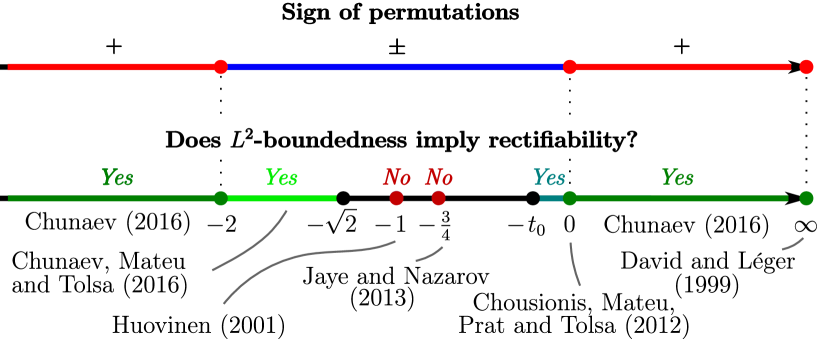
Figure 1. The overall picture for SIO associated with the kernels $k_{t}$

Remark 1.

By simple analysis one can show that the kernel $k_{t}$ has

$$\left\{\begin{array}[]{l}\text{one zero line if }t\in(-\infty,-1)\cup[0,\infty],\\ \text{two zero lines if }t=-1,\\ \text{three zero lines if }t\in(-1,0).\end{array}\right.$$

By a zero line we mean a straight line $L\subset\mathbb{C}$ such that $k_{t}(z)=0$ for $z\in L$.

In this sense, it is interesting to compare Corollary 1 with the part of $(D)$ deduced from [JN]. Observing Figure 1, one can see that the number of zero lines along is not determinant.

Remark 2.

Let $t_{1}$ and $t_{2}$ be such that $-\sqrt{2}\leqslant t_{1}<t_{2}\leqslant-t_{0}$. If there exist finite purely unrectifiable (i.e. concentrated on purely unrectifiable sets) measures $\mu_{1}$ and $\mu_{2}$ with linear growth such that $T_{k_{t_{1}}}$ is $L^{2}(\mu_{1})$-bounded and $T_{k_{t_{2}}}$ is $L^{2}(\mu_{2})$-bounded, then $\mu_{1}$ is different from $\mu_{2}$.

Indeed, let $\mu$ be a finite purely unrectifiable measure with linear growth such that $T_{k_{\tilde{t}}}$ is $L^{2}(\mu)$-bounded for a fixed $\tilde{t}\in[-\sqrt{2},-t_{0}]$. By the triangle inequality for any real $t$,

$$\|T_{k_{t}}1\|_{L^{2}(\mu)}=\|(T_{k_{0}}+(t-\tilde{t})\cdot T_{k_{\infty}}+\tilde{t}\cdot T_{k_{\infty}})1\|_{L^{2}(\mu)}\geqslant|t-\tilde{t}|\|T_{k_{\infty}}1\|_{L^{2}(\mu)}-\|T_{k_{\tilde{t}}}1\|_{L^{2}(\mu)}.$$

Consequently, $\|T_{k_{t}}1\|_{L^{2}(\mu)}=\infty$ for all $t\neq\tilde{t}$ as $\|T_{k_{\infty}}1\|_{L^{2}(\mu)}=\infty$ since $\mu$ is purely unrectifiable. Thus an example of a purely unrectifiable measure $\mu$ such that $T_{k_{\tilde{t}}}$ is $L^{2}(\mu)$-bounded for a fixed $\tilde{t}\in[-\sqrt{2},-t_{0}]$ does not work for $t\neq\tilde{t}$.

2. Notation and definitions

2.1. Constants

We use the letters $c$ and $C$ to denote constants which may change their values at different occurrences. On the other hand, constants with subscripts such as $A_{0}$ or ${\sf c}_{1}$ do not change their values throughout the paper. In a majority of cases constants depend on some parameters which are usually indicated explicitly and will be fixed at the very end so that the constants become absolute.

If there is a constant $C$ such that $A\leqslant C\,B$, we write $A\lesssim B$. Furthermore, $A\approx B$ is equivalent to saying that $A\lesssim B\lesssim A$, possible with different implicit constants. If the implicit constant in expressions with “$\lesssim$” or “$\approx$” depends on some positive parameter, say, $\alpha$, we write $A\lesssim_{\alpha}B$ or $A\approx_{\alpha}B$.

2.2. Curvature and permutations of measure

For an odd and real-valued kernel $K$, consider the following permutations:

(2.1) $$\begin{split}&p_{K}(z_{1},z_{2},z_{3})\\ &:=K(z_{1}-z_{2})K(z_{1}-z_{3})+K(z_{2}-z_{1})K(z_{2}-z_{3})+K(z_{3}-z_{1})K(z_{3}-z_{2}).\end{split}$$

Supposing that $\mu_{1}$, $\mu_{2}$ and $\mu_{3}$ are measures, set

(2.2) $$p_{K}(\mu_{1},\mu_{2},\mu_{3}):=\iiint p_{K}(z_{1},z_{2},z_{3})\;d\mu_{1}(z_{1})\,d\mu_{2}(z_{2})\,d\mu_{3}(z_{3}).$$

We write $p_{K}(\mu):=p_{K}(\mu,\mu,\mu)$ for short and call it permutation of the measure $\mu$. Moreover, in what follows $p_{K,\varepsilon}(\mu_{1},\mu_{2},\mu_{3})$ stands for the integral in the right hand side of (2.2) defined over the set

$$\{(z_{1},z_{2},z_{3})\in\mathbb{C}^{3}:|z_{k}-z_{j}|\geqslant\varepsilon>0,\quad 1\leqslant k,j\leqslant 3,\quad j\neq k\},$$

and $p_{K,\varepsilon}(\mu):=p_{K,\varepsilon}(\mu,\mu,\mu)$.

Identities similar to (2.1) and (2.2) were first considered by Melnikov [M] in the case of the Cauchy kernel $K(z)=1/z$. It can be easily seen that in the related case of $K(z)=\text{\sf Re\,}(1/z)=k_{\infty}(z)$ one has

(2.3) $$p_{k_{\infty}}(z_{1},z_{2},z_{3})=\tfrac{1}{4}c(z_{1},z_{2},z_{3})^{2},$$

where

$$c(z_{1},z_{2},z_{3})=\frac{1}{R(z_{1},z_{2},z_{3})}$$

is the so called Menger curvature and $R(z_{1},z_{2},z_{3})$ stands for the radius of the circle passing through $z_{1}$, $z_{2}$ and $z_{3}$. Clearly, $c(z_{1},z_{2},z_{3})\geqslant 0$ for any $(z_{1},z_{2},z_{3})\in\mathbb{C}^{3}$ which is very important in applications. In what follows, $c^{2}(\mu):=4p_{k_{\infty}}(\mu)$ and $c^{2}_{\varepsilon}(\mu):=4p_{k_{\infty},\varepsilon}(\mu)$ for a measure $\mu$.

The permutations (2.1) and (2.2) for more general kernels $K$ were considered later by Chousionis, Mateu, Prat and Tolsa in [CMPT1] (see also [CMPT2]).

Now let $K$ be an odd real-valued Calderón-Zygmund (i.e. satisfying well-known growth and smoothness conditions) kernel with permutations (2.1), being non-negative for any $(z_{1},z_{2},z_{3})\in\mathbb{C}^{3}$. If $\mu$ has $C_{*}$-linear growth, i.e. there exists a constant $C_{*}>0$ such that

(2.4) $$\mu(B(z,r))\leqslant C_{*}r\qquad\text{for all }r>0\text{ and }z\in\,\mathrm{spt}\,\mu,$$

then the following relation between $p_{K}(\mu)$ and the $L^{2}(\mu)$-norm of $T_{K}1$ holds:

(2.5) $$\|T_{K,\varepsilon}1\|_{L^{2}(\mu)}^{2}=\tfrac{1}{3}p_{K,\varepsilon}(\mu)+\mathcal{R}_{K,\varepsilon}(\mu),\qquad|\mathcal{R}_{K,\varepsilon}(\mu)|\lesssim C_{*}^{2}\mu(\mathbb{C}).$$

An analogous relation was first proved for the Cauchy kernel $K(z)=1/z$. It was done in the seminal paper [MV] by Melnikov and Verdera. It turns out that one can follow Melnikov-Verdera’s proof to obtain the more general identity (2.5) (see, for example, [CMPT1, Lemma 3.3]).

The formulas (2.3) and (2.5), generating the curvature method (also knows as the symmetrization method), are remarkable in the sense that they relate an analytic notion (the operator $T_{K}$, in particular, the Cauchy transform) with a metric-geometric one (permutations, in particular, curvature).

Note that the $L^{2}(\mathcal{H}^{1}\lfloor E)$-boundedness of the Cauchy transform and the identities (2.3) and (2.5) imply that $c^{2}(\mathcal{H}^{1}\lfloor E)<\infty$. Consequently, it is enough to show that $c^{2}(\mathcal{H}^{1}\lfloor E)<\infty$ implies rectifiability. This is actually how it was done in [L].

Take into account that we usually write $p_{t}$ instead of $p_{k_{t}}$ in what follows, in order to simplify notation.

What is more, recall that it is shown in [Ch, Theorem 1 and Remark 1] that

$$\left\{\begin{array}[]{l}p_{t}(z_{1},z_{2},z_{3})\geqslant 0\text{ for any }(z_{1},z_{2},z_{3})\in\mathbb{C}^{3},\text{ if }t\notin(-2,0),\\ p_{t}(z_{1},z_{2},z_{3})\text{ may change sign for some }(z_{1},z_{2},z_{3})\in\mathbb{C}^{3},\text{ if }t\in(-2,0).\end{array}\right.$$

These facts are illustrated in Figure 1. Moreover, by [CMT, Lemma 2],

(2.6) $$p_{0}(z_{1},z_{2},z_{3})\leqslant 2p_{\infty}(z_{1},z_{2},z_{3})\text{ for any }(z_{1},z_{2},z_{3})\in\mathbb{C}^{3}.$$

2.3. Beta numbers and densities

For any closed ball $B=B(x,r)$ with center $x\in\mathbb{C}$ and radius $r>0$ and $1\leqslant p<\infty$, let

(2.7) $$\beta_{\mu,p}(B):=\inf_{L}\left(\frac{1}{r}\int_{B}\left(\frac{\text{\,\rm dist}(y,L)}{r}\right)^{p}\,d\mu(y)\right)^{1/p},$$

where the infimum is taken over all affine lines $L\subset\mathbb{C}$. The $\beta_{\mu,p}$ coefficients were introduced by David and Semmes [DS1] and are the generalization of the well-known Jones $\beta$-numbers [J].

We will mostly deal with $\beta_{\mu,2}(2B_{Q})$ and so by $L_{Q}$ we denote a corresponding best approximating line, i.e. a line where the infimum is reached in (2.7) for $B=2B_{Q}$ (see the definition of $B_{Q}$ below) and $p=2$ .

Throughout the paper we also use the following densities:

$$\Theta_{\mu}(B):=\Theta_{\mu}(x,r)=\dfrac{\mu(B(x,r))}{r},\quad\text{where}\quad B=B(x,r),\qquad x\in{\mathbb{C}},\qquad r>0.$$

3. Main Lemma and proofs of Theorems

Theorem 1 is implied by the following lemma.

Main Lemma.

There exist absolute constants $t_{0}>0$ and $c>0$ such that for any finite measure $\mu$ with $C_{*}$-linear growth it holds that

(3.1) $$p_{\infty}(\mu)\leqslant t_{0}^{-2}p_{0}(\mu)+cC_{*}^{2}\mu(\mathbb{C}).$$

The proof of this result is long and technical and actually takes the biggest part of this paper. Note that (3.1) is a counterpart to the inequality $p_{0}(\mu)\leqslant 2p_{\infty}(\mu)$ that follows from (2.6).

3.1. Proof of Theorem 1

Suppose that Main Lemma holds. Then the identity (2.5) and inequality (3.1) yield

$$\sup_{\varepsilon>0}\|T_{k_{\infty},\varepsilon}1\|_{L^{2}(\mu)}^{2} \leqslant\tfrac{1}{3}p_{{\infty}}(\mu)+cC_{*}^{2}\mu(\mathbb{C})$$

$$\leqslant\tfrac{1}{3}\,t_{0}^{-2}\,p_{{0}}(\mu)+cC_{*}^{2}\mu(\mathbb{C})$$

$$\leqslant t_{0}^{-2}\sup_{\varepsilon>0}\|T_{k_{0},\varepsilon}1\|_{L^{2}(\mu)}^{2}+cC_{*}^{2}\mu(\mathbb{C}),$$

where $c>0$ is an absolute constant. Applying the inequality $\sqrt{ax^{2}+b}\leqslant\sqrt{a}x+\sqrt{b}$ that is valid for $a,b,x\geqslant 0$, gives Theorem 1.

3.2. Proof of Theorem 2

We now apply the perturbation method from [CMT]. By the triangle inequality and Theorem 1,

$$\sup_{\varepsilon>0}\|T_{k_{t},\varepsilon}1\|_{L^{2}(\mu)} =\sup_{\varepsilon>0}\|(T_{k_{0},\varepsilon}+t\cdot T_{k_{\infty},\varepsilon})1\|_{L^{2}(\mu)}$$

$$\geqslant\sup_{\varepsilon>0}\|T_{k_{0},\varepsilon}1\|_{L^{2}(\mu)}-|t|\sup_{\varepsilon>0}\|T_{k_{\infty},\varepsilon}1\|_{L^{2}(\mu)}$$

$$\geqslant(t_{0}-|t|)\sup_{\varepsilon>0}\|T_{k_{\infty},\varepsilon}1\|_{L^{2}(\mu)}-cC_{*}\sqrt{\mu(\mathbb{C})}.$$

Consequently,

$$\sup_{\varepsilon>0}\|T_{k_{\infty},\varepsilon}1\|_{L^{2}(\mu)}\leqslant\frac{\sup_{\varepsilon>0}\|T_{k_{t},\varepsilon}1\|_{L^{2}(\mu)}+cC_{*}\sqrt{\mu(\mathbb{C})}}{t_{0}-|t|},\qquad|t|<t_{0}.$$

Therefore, given any cube $Q\subset\mathbb{C}$, applying this estimate to the measure $\mu\lfloor Q$, we get

(3.2) $$\sup_{\varepsilon>0}\|T_{k_{\infty},\varepsilon}\chi_{Q}\|_{L^{2}(\mu\lfloor Q)}\leqslant\frac{\sup_{\varepsilon>0}\|T_{k_{t},\varepsilon}\chi_{Q}\|_{L^{2}(\mu\lfloor Q)}+cC_{*}\sqrt{\mu(Q)}}{t_{0}-|t|},\qquad|t|<t_{0}.$$

By a variant of the $T1$ Theorem of Nazarov, Treil and Volberg from [T3, Theorem 9.40], we infer from (3.2) that the $L^{2}(\mu)$-boundedness of $T_{k_{t}}$ with a fixed $t$ such that $|t|<t_{0}$ implies that of $T_{k_{\infty}}$, and thus the Cauchy transform is $L^{2}(\mu)$-bounded.

4. Other corollaries

Recall that a measure $\mu$ is Ahlfors-David regular (AD-regular) if

$$C^{-1}r\leqslant\mu(B(z,r))\leqslant Cr,\qquad\text{where}\qquad z\in\,\mathrm{spt}\,\mu,\qquad 0<r<\text{\,\rm diam}(\,\mathrm{spt}\,\mu),$$

and $C>1$ is some fixed constant. A measure $\mu$ is called uniformly rectifiable if it is AD-regular and $\,\mathrm{spt}\,\mu$ is contained in an AD-regular curve. One can summarise all up-to-date results characterising uniformly rectifiable measures via $L^{2}(\mu)$-bounded SIOs $T_{k_{t}}$ as follows.

Corollary 2.

Let $\mu$ be an AD-regular measure and $t\in(-\infty,-\sqrt{2})\cup(-t_{0},\infty]$. The measure $\mu$ is uniformly rectifiable if and only if the SIO $T_{k_{t}}$ is $L^{2}(\mu)$-bounded.

The part of Corollary 2 for $t=\infty$, i.e. for the Cauchy transform, was proved in [MMV]; for $t=0$ in [CMPT1]; and for $t\in(-\infty,-\sqrt{2})\cup(0,\infty)$ in [Ch, CMT].

Furthermore, one can formulate the following general result.

Corollary 3.

Let $\mu$ be a measure with linear growth and $t\in(-\infty,-\sqrt{2})\cup(-t_{0},\infty]$. If the SIO $T_{k_{t}}$ is $L^{2}(\mu)$-bounded, then so are all $1$-dimensional SIOs associated with a wide class of sufficiently smooth kernels kernels.

We refer the reader to [T1, Sections 1 and 12] and [G, Theorem A] for the more precise description of what is meant by “sufficiently smooth kernels”.

The part of Corollary 3 for $t=\infty$, i.e. for the Cauchy transform, was proved in [T1] (see also [G]) and for $t\in(-\infty,-\sqrt{2})\cup(0,\infty)$ in [Ch, CMT].

5. Plan of the proof of Main Lemma

To prove Main Lemma, we will use a corona decomposition that is similar, for example, to the ones from [T4] and [AT]: it splits the David-Mattila dyadic lattice into some collections of cubes, which we will call “trees”, where the density of $\mu$ does not oscillate too much and most of the measure is concentrated close to a graph of a Lipschitz function. To construct this function we will use a variant of the Whitney extension theorem adapted to the David-Mattila dyadic lattice. Further, we will show that the family of trees of the corona decomposition satisfies a packing condition by arguments inspired by some of the techniques used in [AT] and earlier in [T2] to prove the bilipschitz “invariance” of analytic capacity. More precisely, we will deduce Main Lemma from the two-sided estimate

(5.1) $$p_{k_{\infty}}(\mu)\lesssim\sum_{R\in{\sf Top}}\Theta_{\mu}(2B_{R})^{2}\mu(R)\lesssim p_{k_{0}}(\mu)+C_{*}^{2}\mu(\mathbb{C}),$$

where ${\sf Top}$ is the family of top cubes for the above-mentioned trees. Note that the left hand side inequality in (5.1) in essentially contained in [T4] and verifying the right hand side inequality is actually the main objective in the proof.

It is worth mentioning that the structure of our trees is more complicated than in [AT]. This is because we deal with permutations which are not comparable to curvature in some cases and this leads to additional technical difficulties. What is more, we are not able to use a nice theorem by David and Toro [DT] which shortens the proof in [AT] considerably. Indeed, this theorem would be useful to construct a chordal curve such that most of the measure $\mu$ is concentrated close to it. However, in our situation we need to control slope and therefore we have to deal with and to construct a graph of a Lipschitz function with well-controlled Lipschitz constant instead.

The plan of the proof of Main Lemma is the following. In Section 6 we recall the properties of the David-Mattila dyadic lattice. We construct the trees and establish their properties in Sections 7–13. The main properties are summarized in Section 14, where they are further used for constructing the corona type decomposition. The end of the proof of Main Lemma is given in Section 14.6.

Finally, in Section 15 we show how one can slightly change the proof of Main Lemma in order to give another proof of a certain result from [AT] and obtain an alternative proof of the bi-Lipschitz invariance of the $L^{2}$-boundedness of the Cauchy transform.

Remark 3.

The measure $\mu$ considered below is under assumptions of Main Lemma, i.e. $\mu$ is a finite measure with $C_{*}$-linear growth. Moreover, without loss of generality we additionally suppose that $\mu$ has compact support.

6. The David-Mattila lattice

We use the dyadic lattice of cubes with small boundaries constructed by David and Mattila [DM]. The properties of this lattice are summarized in the next lemma (for the case of $\mathbb{C}$).

Lemma 1 (Theorem 3.2 in [DM]).

Let $\mu$ be a measure, $E=\,\mathrm{spt}\,\mu$, and consider two constants $C_{0}>1$ and $A_{0}>5000\,C_{0}$. Then there exists a sequence of partitions of $E$ into Borel subsets $Q$, $Q\in\mathcal{D}_{k}$, with the following properties:

• For each integer $k\geqslant 0$, $E$ is the disjoint union of the “cubes” $Q$, $Q\in\mathcal{D}_{k}$, and if $k<l$, $Q\in\mathcal{D}_{l}$, and $R\in\mathcal{D}_{k}$, then either $Q\cap R=\varnothing$ or else $Q\subset R$.

• The general position of the cubes $Q$ can be described as follows. For each $k\geqslant 0$ and each cube $Q\in\mathcal{D}_{k}$, there is a ball $B(Q)=B(z_{Q},r(Q))$ such that

  $$z_{Q}\in Q,\qquad A_{0}^{-k}\leqslant r(Q)\leqslant C_{0}\,A_{0}^{-k},$$

  $$E\cap B(Q)\subset Q\subset E\cap 28\,B(Q)=E\cap B(z_{Q},28r(Q)),$$

  and

  the balls $$5B(Q) Q\in\mathcal{D}_{k}$$, , are disjoint.

• The cubes $Q\in\mathcal{D}_{k}$ have small boundaries. That is, for each $Q\in\mathcal{D}_{k}$ and each integer $l\geqslant 0$, set

  $$N_{l}^{ext}(Q)=\{x\in E\setminus Q:\,\text{\,\rm dist}(x,Q)<A_{0}^{-k-l}\},$$

  $$N_{l}^{int}(Q)=\{x\in Q:\,\text{\,\rm dist}(x,E\setminus Q)<A_{0}^{-k-l}\},$$

  and

  $$N_{l}(Q)=N_{l}^{ext}(Q)\cup N_{l}^{int}(Q).$$

  Then

  $$\mu(N_{l}(Q))\leqslant(C^{-1}C_{0}^{-7}A_{0})^{-l}\,\mu(90B(Q)).$$

• Denote by $\mathcal{D}_{k}^{db}$ the family of cubes $Q\in\mathcal{D}_{k}$ for which

  (6.1) $$\mu(100B(Q))\leqslant C_{0}\,\mu(B(Q)).$$

  If $Q\in\mathcal{D}_{k}\setminus\mathcal{D}_{k}^{db}$, then $r(Q)=A_{0}^{-k}$ and

  $$\mu(100B(Q))\leqslant C_{0}^{-l}\,\mu(100^{l+1}B(Q))\quad\mbox{for all $l\geqslant 1$ such that $100^{l}\leqslant C_{0}$.}$$

We use the notation $\mathcal{D}=\bigcup_{k\geqslant 0}\mathcal{D}_{k}$. For $Q\in\mathcal{D}$, we set $\mathcal{D}(Q)=\{P\in\mathcal{D}:P\subset Q\}$. Observe that

$$r(Q)\approx\text{\,\rm diam}(Q).$$

Also we call $z_{Q}$ the center of $Q$. We set $B_{Q}=28\,B(Q)=B(z_{Q},28\,r(Q))$, so that

$$E\cap\tfrac{1}{28}B_{Q}\subset Q\subset B_{Q}.$$

We denote $\mathcal{D}^{db}=\bigcup_{k\geqslant 0}\mathcal{D}_{k}^{db}$ and $\mathcal{D}^{db}(Q)=\mathcal{D}^{db}\cap\mathcal{D}(Q)$. Note that, in particular, from (6.1) it follows that

(6.2) $$\mu(100B(Q))\leqslant C_{0}\,\mu(2B_{Q})\qquad\text{if }Q\in\mathcal{D}^{db}.$$

For this reason we will call the cubes from $\mathcal{D}^{db}$ doubling.

As shown in [DM], any cube $Q\in\mathcal{D}$ can be covered $\mu$-a.e. by doubling cubes.

Lemma 2 (Lemma 5.28 in [DM]).

Let $Q\in\mathcal{D}$. Suppose that the constants $A_{0}$ and $C_{0}$ in Lemma 1 are chosen suitably. Then there exists a family of doubling cubes $\{Q_{i}\}_{i\in I}\subset\mathcal{D}^{db}$, with $Q_{i}\subset Q$ for all $i$, such that their union covers $\mu$-almost all $Q$.

We denote by $J(Q)$ the number $k$ such that $Q\in\mathcal{D}_{k}$.

Lemma 3 (Lemma 5.31 in [DM]).

Let $P\in\mathcal{D}$ and let $Q\subsetneq P$ be a cube such that all the intermediate cubes $S$, $Q\subsetneq S\subsetneq P$, are non-doubling $($i.e. not in $\mathcal{D}^{db}$$)$. Then

$$\mu(100B(Q))\leqslant A_{0}^{-20(J(Q)-J(P)-1)}\mu(100B(P)).$$

Recall that $\Theta_{\mu}(B)=\mu(B(x,r))/r$. From Lemma 3 one can easily deduce

Lemma 4 (Lemma 2.4 in [AT]).

Let $Q,P\in\mathcal{D}$ be as in Lemma 3. Then

$$\Theta_{\mu}(100B(Q))\leqslant C_{0}A_{0}^{-19(J(Q)-J(P)-1)+1}\,\Theta_{\mu}(100B(P))\leqslant C_{0}A_{0}\,\Theta_{\mu}(100B(P))$$

and

$$\sum_{S\in\mathcal{D}:Q\subset S\subset P}\Theta_{\mu}(100B(S))\leqslant c\,\Theta_{\mu}(100B(P)),\qquad c=c(C_{0},A_{0}).$$

We will assume that all implicit constants in the inequalities that follow may depend on $C_{0}$ and $A_{0}$. Moreover, we will assume that $C_{0}$ and $A_{0}$ are some big fixed constants so that the results stated in the lemmas below hold.

7. Balanced cubes and control on beta numbers through permutations

We first recall the properties of the so called balanced balls introduced in [AT].

Lemma 5 (Lemma 3.3 and Remark 3.2 in [AT]).

Let $\mu$ be a measure and consider the dyadic lattice $\mathcal{D}$ associated with $\mu$ from Lemma 1. Let ${0<\gamma<1}$ be small enough $($with respect to some absolute constant$)$, then there exist $\rho^{\prime}=\rho^{\prime}(\gamma)>0$ and $\rho^{\prime\prime}=\rho^{\prime\prime}(\gamma)>0$ such that one of the following alternatives holds for every $Q\in\mathcal{D}^{db}$:

• There are balls $B_{k}=B(\xi_{k},\rho^{\prime}\,r(Q))$, $k=1,2$, where $\xi_{1},\xi_{2}\in B(Q)$, such that

  $$\mu\left(B_{k}\cap B(Q)\right)\geqslant\rho^{\prime\prime}\,\mu(Q),\qquad k=1,2,$$

  and for any $y_{k}\in B_{k}\cap Q$, $k=1,2$,

  $$\text{\,\rm dist}(y_{1},y_{2})\geqslant\gamma\,r(B_{Q}).$$

• There exists a family of pairwise disjoint cubes $\{P\}_{P\in I_{Q}}\subset\mathcal{D}^{db}(Q)$ so that $\text{\,\rm diam}(P)\gtrsim\gamma\text{\,\rm diam}(Q)$ and $\Theta_{\mu}(2B_{P})\gtrsim\gamma^{-1}\,\Theta_{\mu}(2B_{Q})$ for each $P\in I_{Q}$, and

  (7.1) $$\sum_{P\in I_{Q}}\Theta_{\mu}(2B_{P})^{2}\,\mu(P)\gtrsim\gamma^{-2}\,\Theta_{\mu}(2B_{Q})^{2}\,\mu(Q).$$

Let us mention that the densities in the latter inequality in the original Lemma 3.3 in [AT] are not squared. However, a slight variation of the proof of [AT, Lemma 3.3] gives (7.1) as stated.

Moreover, notice that in Lemma 5 the cubes $Q$ and $P$, with $P\in I_{Q}$, are doubling. If the alternative $(a)$ holds for a doubling cube $Q$ with some $\gamma$, $\rho^{\prime}(\gamma)$ and $\rho^{\prime\prime}(\gamma)$, then the corresponding ball $B(Q)$ is called $\gamma$-balanced. Otherwise, it is called $\gamma$-unbalanced. If $B(Q)$ is $\gamma$-balanced, then the cube $Q$ is also called $\gamma$-balanced.

We are going to show now that the beta numbers $\beta_{\mu,2}(2B_{Q})$ (see (2.7)) for $\gamma$-balanced cubes $Q$ are controlled by a truncated version of the permutations $p_{0}(\mu\lfloor 2B_{Q})$. To do so, we introduce some additional notation.

Given two distinct points $z,w\in\mathbb{C}$, we denote by $L_{z,w}$ the line passing through $z$ and $w$. Given three pairwise distinct points $z_{1},z_{2},z_{3}\in\mathbb{C}$, we denote by $\measuredangle(z_{1},z_{2},z_{3})$ the smallest angle formed by the lines $L_{z_{1},z_{2}}$ and $L_{z_{1},z_{3}}$ and belonging to $[0,\pi/2]$. If $L$ and $L^{\prime}$ are lines, let $\measuredangle(L,L^{\prime})$ be the smallest angle between them. This angle belongs to $[0,\pi/2]$, too. Also, we set $\theta_{V}(L)=\measuredangle(L,V)$, where $V$ is the vertical line.

First we recall the following result of Chousionis and Prat [CP]. We say that a triple $(z_{1},z_{2},z_{3})\in\mathbb{C}^{3}$ is in the class ${\rm V}_{\sf Far}(\theta)$ if it satisfies

(7.2) $$\theta_{V}(L_{z_{1},z_{2}})+\theta_{V}(L_{z_{1},z_{3}})+\theta_{V}(L_{z_{2},z_{3}})\geqslant\theta>0.$$

Lemma 6 (Proposition 3.3 in [CP]).

If $(z_{1},z_{2},z_{3})\in{\rm V}_{\sf Far}(\theta)$, then

(7.3) $$p_{0}(z_{1},z_{2},z_{3})\geqslant{\sf c_{1}}(\theta)\cdot p_{\infty}(z_{1},z_{2},z_{3}),\quad\text{where}\quad 0<{\sf c_{1}}(\theta)\leqslant 2.$$

Note that the inequality ${\sf c_{1}}(\theta)\leqslant 2$ follows from (2.6) that was proved in [CMT].

For measures $\mu_{1}$, $\mu_{2}$ and $\mu_{3}$ and a cube $Q$ we set

$$p^{[\delta,Q]}_{0}(\mu_{1},\mu_{2},\mu_{3}):=\iiint\limits_{\delta r(Q)\leqslant|z_{1}-z_{2}|\leqslant\delta^{-1}r(Q)}p_{0}(z_{1},z_{2},z_{3})\;d\mu_{1}(z_{1})d\mu_{2}(z_{2})d\mu_{3}(z_{3}).$$

The parameter $\delta>0$ will be chosen later to be small enough for our purposes. If $\mu_{1}=\mu_{2}=\mu_{3}=\mu$, then we write $p^{[\delta,Q]}_{0}(\mu)$ instead of $p^{[\delta,Q]}_{0}(\mu,\mu,\mu)$, for short.

Now we are ready to state the above mentioned estimate of $\beta_{\mu,2}(2B_{Q})$ for $\gamma$-balanced cubes $Q$ via the truncated version of $p_{0}(\mu\lfloor 2B_{Q})$. Pay attention that the first term in the estimate is a “non-summable” part which makes a big difference with the case of curvature or $p_{\infty}$ (see Section 15).

Lemma 7.

If $Q$ is $\gamma$-balanced, then for any $\varepsilon\in(0,1)$,

(7.4) $$\beta_{\mu,2}(2B_{Q})^{2}\Theta_{\mu}(2B_{Q})\leqslant 4\varepsilon^{2}\Theta_{\mu}(2B_{Q})^{2}+C(\varepsilon,\gamma)\frac{p^{[\delta,Q]}_{0}(\mu\lfloor 2B_{Q})}{\mu(Q)},\qquad 0<\delta\leqslant\gamma.$$

Moreover, for any $\varepsilon_{0}>0$, there exist $\varepsilon=\varepsilon(\varepsilon_{0})>0$ and $\tilde{\varepsilon}=\tilde{\varepsilon}(\varepsilon_{0},\gamma)>0$ such that if

(7.5) $$\frac{p^{[\delta,Q]}_{0}(\mu\lfloor 2B_{Q})}{\Theta_{\mu}(2B_{Q})^{2}\mu(Q)}\leqslant\tilde{\varepsilon},$$

then

$$\beta_{\mu,2}(2B_{Q})^{2}\leqslant\varepsilon_{0}^{2}\Theta_{\mu}(2B_{Q}).$$

Proof.

By Lemma 5, there exist balls $B_{k}=B(\xi_{k},\rho^{\prime}\,r(Q))$, $k=1,2$, where $\xi_{k}\in B(Q)$, such that $\mu(B_{k}\cap B(Q))\geqslant\rho^{\prime\prime}\mu(Q)$ and $\text{\,\rm dist}(y_{1},y_{2})\geqslant\gamma r(B_{Q})$ for any $y_{k}\in B_{k}\cap Q$, $k=1,2$. From (2.7) it follows that

$$\beta_{\mu,2}(2B_{Q})^{2} \leqslant\frac{1}{2r(B_{Q})}\int_{2B_{Q}}\bigg{(}\frac{\text{\,\rm dist}(w,L_{y_{1},y_{2}})}{2r(B_{Q})}\bigg{)}^{2}d\mu(w).$$

We separate triples $(w,y_{1},y_{2})$ that are in and not in ${\rm V}_{\sf Far}(\varepsilon)$. Clearly,

$$\text{\,\rm dist}(w,L_{y_{1},y_{2}})\leqslant\text{\,\rm diam}(2B_{Q})\sin\varepsilon\leqslant 4\,\varepsilon\,r(B_{Q})\qquad\text{if }(w,y_{1},y_{2})\notin{\rm V}_{\sf Far}(\varepsilon).$$

Thus

$$\beta_{\mu,2}(2B_{Q})^{2}$$

$$\quad\leqslant\frac{4\varepsilon^{2}}{2r(B_{Q})}\int_{2B_{Q}}d\mu(w)+\frac{1}{2r(B_{Q})}\int_{2B_{Q},\;(w,y_{1},y_{2})\in{\rm V}_{\sf Far}(\varepsilon)}\bigg{(}\frac{\text{\,\rm dist}(w,L_{y_{1},y_{2}})}{2r(B_{Q})}\bigg{)}^{2}d\mu(w)$$

$$\quad\leqslant 4\varepsilon^{2}\Theta_{\mu}(2B_{Q})+8r(B_{Q})\int_{2B_{Q},\;(w,y_{1},y_{2})\in{\rm V}_{\sf Far}(\varepsilon)}\bigg{(}\frac{2\text{\,\rm dist}(w,L_{y_{1},y_{2}})}{|w-y_{1}||w-y_{2}|}\bigg{)}^{2}d\mu(w)$$

$$\quad=4\varepsilon^{2}\Theta_{\mu}(2B_{Q})+8r(B_{Q})\int_{\,2B_{Q},\;(w,y_{1},y_{2})\in{\rm V}_{\sf Far}(\varepsilon)}c(w,y_{1},y_{2})^{2}d\mu(w).$$

We used that $|w-y_{k}|\leqslant\text{\,\rm diam}(2B_{Q})=4r(B_{Q})$ as $w,y_{1},y_{2}\in 2B_{Q}$ and that

$$c(w,y_{1},y_{2})=\frac{2\text{\,\rm dist}(w,L_{y_{1},y_{2}})}{|w-y_{1}||w-y_{2}|}.$$

Recall that $r(B_{Q})=28r(Q)$ by definition. By (2.3) and (7.3),

$$\int_{\,2B_{Q},\;(w,y_{1},y_{2})\in{\rm V}_{\sf Far}(\varepsilon)}c(w,y_{1},y_{2})^{2}d\mu(w)$$

$$\qquad\qquad\qquad\leqslant\frac{2}{{\sf c_{1}}(\varepsilon)}\int_{\,2B_{Q},\;(w,y_{1},y_{2})\in{\rm V}_{\sf Far}(\varepsilon)}p_{0}(w,y_{1},y_{2})d\mu(w).$$

Recall that $|y_{1}-y_{2}|\geqslant\gamma r(Q)$ for any $y_{k}\in B_{k}\cap Q$, $k=1,2$. Furthermore, for any $\delta$ such that $0<\delta\leqslant\gamma$ we can find $y_{1}\in B_{1}$ and $y_{2}\in B_{2}$ so that

$$\int_{2B_{Q}}p_{0}(w,y_{1},y_{2})d\mu(w)\leqslant\frac{p^{[\delta,Q]}_{0}(\mu\lfloor 2B_{Q})}{\mu(B_{1})\mu(B_{2})}\leqslant\frac{p^{[\delta,Q]}_{0}(\mu\lfloor 2B_{Q})}{(\rho^{\prime\prime})^{2}\mu(Q)^{2}}.$$

By (6.1) and the fact that $E\cap B(Q)\subset Q$, we deduce that

$$\mu(Q)\geqslant C_{0}^{-1}\mu(100B(Q))\geqslant C_{0}^{-1}\mu(56B(Q))=C_{0}^{-1}\mu(2B_{Q}).$$

Consequently,

$$\beta_{\mu,2}(2B_{Q})^{2} \leqslant 4\varepsilon^{2}\Theta_{\mu}(2B_{Q})+\frac{16r(B_{Q})p^{[\delta,Q]}_{0}(\mu\lfloor 2B_{Q})}{{\sf c_{1}}(\varepsilon)(\rho^{\prime\prime})^{2}\mu(Q)C_{0}^{-1}\mu(2B_{Q})}$$

$$=4\varepsilon^{2}\Theta_{\mu}(2B_{Q})+C(\varepsilon,\gamma)\frac{p^{[\delta,Q]}_{0}(\mu\lfloor 2B_{Q})}{\Theta_{\mu}(2B_{Q})\mu(Q)}.$$

Multiplying both sides by $\Theta_{\mu}(2B_{Q})$ finishes the proof of (7.4). Note that $\rho^{\prime\prime}=\rho^{\prime\prime}(\gamma)$.

Let us prove the second statement. By the assumption (7.5),

$$\beta_{\mu,2}(2B_{Q})^{2}\leqslant(4\varepsilon^{2}+C(\varepsilon,\gamma)\tilde{\varepsilon})\Theta_{\mu}(2B_{Q}).$$

For any $\varepsilon_{0}>0$, we put $\varepsilon=\tfrac{\sqrt{2}}{4}\varepsilon_{0}$ and choose $\tilde{\varepsilon}$ so that $\tilde{\varepsilon}\leqslant\tfrac{1}{2}\varepsilon_{0}^{2}/C(\varepsilon,\gamma)$. ∎

8. Parameters and thresholds

Recall that we work everywhere with the David-Mattila dyadic lattice $\mathcal{D}$ associated with the measure $\mu$.

In what follows we will use many parameters and thresholds. Some of them depend on each other, some are independent. Let us give a list of the parameters:

• $\tau$ is the threshold for cubes with low density:

  $$0<\tau\ll 1.$$

• $A$ is the threshold for cubes with high density:

  $$0<A^{-1}\leqslant\tau^{2}\ll 1,\quad\text{i.e.}\quad A\gg 1.$$

• $\theta_{0}$ is the threshold for the angle between best approximating lines associated to some cubes:

  $$0<\theta_{0}\ll 1.$$

• $\gamma$ is the parameter controlling unbalanced cubes:

  $$0<\gamma\leqslant\tau^{3}\ll 1.$$

• $\varepsilon_{0}$ is the threshold controlling the $\beta_{2,\mu}$-numbers:

  $$0<\varepsilon_{0}=\varepsilon_{0}(\gamma,\tau,A,\theta_{0})\ll 1.$$

• $\alpha$ is the threshold controlling permutations of intermediate cubes:

  $$0<\alpha=\alpha(\tau,A,\varepsilon_{0},\gamma,\theta_{0})\ll 1.$$

• $\delta$ is the parameter controlling the truncation of permutations:

  $$0<\delta=\delta(\gamma,\varepsilon_{0},\tau,A)\ll 1.$$

All the parameters and thresholds are supposed to be chosen (and fixed at the very end) so that the forthcoming results hold true. In what follows, we will again indicate step by step how the choice should be made.

9. Stopping cubes and trees

9.1. Stopping cubes

Let $R\in\mathcal{D}^{db}$. We use the parameters and thresholds given in Section 8. We denote by ${\sf Stop}(R)$ the family of the maximal cubes $Q\subset R$ for which one of the following holds:

1. $Q\in{\mathsf{HD}}(R)\cup{\mathsf{LD}}(R)\cup{\sf UB}(R)$, where

   • ${\mathsf{HD}}(R)$ is the family of high density doubling cubes $Q\in\mathcal{D}^{db}$ satisfying

     $$\Theta_{\mu}(2B_{Q})>A\,\Theta_{\mu}(2B_{R});$$

   • ${\mathsf{LD}}(R)$ is the family of low density cubes $Q$ satisfying

     $$\Theta_{\mu}(2B_{Q})<\tau\,\Theta_{\mu}(2B_{R});$$

   • ${\sf UB}(R)$ is the family of unbalanced cubes $Q\in\mathcal{D}^{db}\setminus({\mathsf{HD}}(R)\cup{\mathsf{LD}}(R))$ such that $Q$ is $\gamma$-unbalanced;

2. $Q\in\mathsf{BP}(R)$ (“big permutations”), meaning $Q\notin{\mathsf{HD}}(R)\cup{\mathsf{LD}}(R)\cup{\sf UB}(R)$ and

   $$\sum_{Q\subset\tilde{Q}\subset R}\textsf{perm}(\tilde{Q})^{2}>\alpha^{2},\qquad\textsf{perm}(\tilde{Q})^{2}:=\frac{p_{0}^{[\delta,\tilde{Q}]}(\mu\lfloor 2B_{\tilde{Q}},\mu\lfloor 2B_{R},\mu\lfloor 2B_{R})}{\Theta_{\mu}(2B_{R})^{2}\mu(\tilde{Q})}.$$

3. $Q\in\mathsf{BS}(R)$ (“big slope”), meaning $Q\notin{\mathsf{HD}}(R)\cup{\mathsf{LD}}(R)\cup{\sf UB}(R)\cup\mathsf{BP}(R)$ and $Q\in\mathcal{D}^{db}$ so that

   $$\measuredangle(L_{Q},L_{R})>\theta(R),$$

   where $\theta(R)$ depends on some geometric properties of $R$ and is comparable with the parameter $\theta_{0}>0$ mentioned in Section 8. The more precise description will be given in Section 13.

4. $Q\in\textsf{F}(R)$ (“big part of $Q$ is far from best approximating lines for the doubling ancestors of $Q$”), meaning $Q\notin{\mathsf{HD}}(R)\cup{\mathsf{LD}}(R)\cup{\sf UB}(R)\cup\mathsf{BP}(R)\cup\mathsf{BS}(R)$ and

   $$\mu(Q\setminus 2B_{Q}^{\sf Cl})>\sqrt{\alpha}\,\mu(Q),$$

   where

   (9.1) $$\begin{split}2B_{Q}^{\sf Cl}:=\{&x\in R\cap 2B_{Q}:\;\text{\,\rm dist}(x,L_{\tilde{Q}})\leqslant 5\sqrt{\varepsilon_{0}}\,r(B_{\tilde{Q}})\quad\forall\tilde{Q}\in\mathcal{D}^{db}(R)\,:\\ &2B_{Q}\subset 2B_{\tilde{Q}}\text{ and }\tilde{Q}\text{ is not contained in any cube from }\\ &{\mathsf{HD}}(R)\cup{\mathsf{LD}}(R)\cup{\sf UB}(R)\cup\mathsf{BP}(R)\cup\mathsf{BS}(R)\}.\end{split}$$

Let ${\sf Tree}(R)$ be the subfamily of the cubes from $\mathcal{D}(R)$ which are not strictly contained in any cube from ${\sf Stop}(R)$. We also set

$${\sf DbTree}(R):=\mathcal{D}^{db}\cap({\sf Tree}(R)\setminus{\sf Stop}(R)).$$

Note that all cubes in ${\sf Stop}(R)$ are disjoint.

Remark 4.

It may happen that ${\sf Stop}(R)$ is empty. In this case there is no need to estimate the measure of stopping cubes and we may immediately go to Section 11. In the lemmas below related to estimating the measure of stopping cubes we naturally suppose that ${\sf Stop}(R)$ is not empty.

Generally speaking it is possible that $R\in{\sf Stop}(R)$ (and then ${\sf DbTree}(R)$ is empty). Clearly, $R\notin\textsf{HD}(R)\cup\textsf{LD}(R)\cup{\sf BS}(R)$ by definition but it may occur that $R\in\textsf{UB}(R)\cup\textsf{BP}(R)\cup\textsf{F}(R)$. Firstly, we will not work with the family ${\sf UB}(R)$ before Section 14 so we may assume before that section that $R\notin{\sf UB}(R)$. Secondly, if $R\in{\sf BP}(R)$, then we may directly go to Lemma 14 and use the same estimate for the measure of stopping cubes from ${\sf BP}(R)$. Thirdly, it will follow from Lemmas 12 and 13 (see Remark 5) that if $R\notin{\sf UB}(R)\cup{\sf BP}(R)$, then $R\notin{\sf F}(R)$, i.e. the case $R\in{\sf F}(R)$ may be skipped.

It is also worth mentioning that if $R\in{\sf Stop}(R)$, then the Lipschitz function mentioned in Section 5 may be chosen identically zero and its graph is just $L_{R}$.

9.2. Properties of cubes in trees

Below, we will collect main properties of cubes from ${\sf Tree}(R)$ that readily follow from the stopping conditions. Before it we prove an additional result.

Lemma 8.

For any $Q\in{\sf Tree}(R)$, we have

$$\Theta_{\mu}(2B_{Q})\lesssim A\,\Theta_{\mu}(2B_{R}).$$

The implicit constant depends only on $C_{0}$ and $A_{0}$.

Proof.

Let $Q\in{\sf Tree}(R)$. If $Q\in\mathcal{D}^{db}$, then there is nothing to prove. If not, then denote by $\tilde{Q}\in\mathcal{D}^{db}$ the first doubling ancestor of $Q$. Such a cube $\tilde{Q}$ exists and $\tilde{Q}\subset R$ because $R\in\mathcal{D}^{db}$ by construction. Since the intermediate cubes $P$, $Q\subsetneq P\subsetneq\tilde{Q}$, do not belong to $\mathcal{D}^{db}$, by Lemma 4 we have

$$\Theta_{\mu}(2B_{Q})\lesssim\Theta_{\mu}(100B(Q))\lesssim C_{0}A_{0}\Theta_{\mu}(100B(\tilde{Q})).$$

Using that $\tilde{Q}\in\mathcal{D}^{db}$, namely, the inequality (6.2), we get

$$\Theta_{\mu}(2B_{Q})\lesssim C_{0}^{2}A_{0}\,\Theta_{\mu}(2B_{\tilde{Q}})\lesssim C_{0}^{2}A_{0}\,A\,\Theta_{\mu}(2B_{R}),$$

and we are done. ∎

Lemma 9.

The following properties hold:

(9.2) $$\tau\,\Theta_{\mu}(2B_{R})\leqslant\Theta_{\mu}(2B_{Q})\lesssim A\,\Theta_{\mu}(2B_{R}),\quad\forall Q\in{\sf Tree}(R)\setminus({\sf LD}(R)\cup{\sf HD}(R)).$$

(9.3) $$Q\in\mathcal{D}^{db}\cap({\sf Tree}(R)\setminus({\sf HD}(R)\cup{\sf LD}(R)\cup{\sf UB}(R)))\quad\Longrightarrow\quad\text{$Q$ is $\gamma$-balanced}.$$

(9.4) $$\sum_{Q\subset\tilde{Q}\subset R}{\sf perm}(\tilde{Q})^{2}<\alpha^{2}\quad\forall Q\in{\sf Tree}(R)\setminus({\sf HD}(R)\cup{\sf LD}(R)\cup{\sf UB}(R)\cup{\sf BP}(R)).$$

(9.5) $$\begin{split}&\beta_{\mu,2}(2B_{Q})^{2}\leqslant\varepsilon_{0}^{2}\Theta_{\mu}(2B_{Q})\quad\text{ if }\alpha=\alpha(\gamma,\tau,\varepsilon_{0})\text{ is small enough and}\\ &Q\in\mathcal{D}^{db}\cap({\sf Tree}(R)\setminus({\sf HD}(R)\cup{\sf LD}(R)\cup{\sf UB}(R)\cup{\sf BP}(R))).\end{split}$$

(9.6) $$\measuredangle(L_{Q},L_{R})\leqslant\theta(R)\qquad\forall Q\in{\sf DbTree}(R).$$

(9.7) $$\mu(Q\setminus 2B_{Q}^{\sf Cl})\leqslant\sqrt{\alpha}\,\mu(Q)\qquad\forall Q\in{\sf Tree}(R)\setminus{\sf Stop}(R).$$

Proof.

The statement (9.2) follows from Lemma 8 and the stopping condition (S1). The statements (9.3), (9.4), (9.6) and (9.7) immediately follow from the construction of ${\sf Stop}(R)$ and ${\sf Tree}(R)$, while (9.5) is implied by Lemma 7 and the stopping conditions (S1) and (S2). ∎

The following property of $\gamma$-balanced cubes will be used many times below.

Lemma 10.

Let $\varepsilon_{0}=\varepsilon_{0}(\gamma)$ be chosen small enough. Then for any $Q\in\mathcal{D}^{db}\cap({\sf Tree}(R)\setminus({\sf HD}(R)\cup{\sf LD}(R)\cup{\sf UB}(R)\cup{\sf BP}(R)))$ there exist two sets $\mathcal{Z}_{k}\subset Q$, $k=1,2$, such that

$$\mu(Q)\lesssim_{\gamma}\mu(\mathcal{Z}_{k})\leqslant\mu(Q)\quad\text{and}\quad\text{\,\rm dist}(\mathcal{Z}_{1},\mathcal{Z}_{2})\geqslant\gamma r(B_{Q}),$$

and moreover for any $z_{1}\in\mathcal{Z}_{1}$ and $z_{2}\in\mathcal{Z}_{2}$ we have

$$\text{\,\rm dist}_{H}(L_{z_{1},z_{2}}\cap 2B_{Q},L_{Q}\cap 2B_{Q})\leqslant\sqrt{\varepsilon_{0}}\,r(B_{Q}).$$

Proof.

Since $Q\in\mathcal{D}^{db}\cap({\sf Tree}(R)\setminus({\sf HD}(R)\cup{\sf LD}(R)\cup{\sf UB}(R)))$, $Q$ is $\gamma$-balanced by (9.3). Furthermore, by Lemma 5 there exist balls $B_{k}=B(\xi_{k},\rho^{\prime}r(Q))$, $k=1,2$, where $\xi_{k}\in B(Q)$, such that

$$\mu(B_{k}\cap B(Q))\geqslant\rho^{\prime\prime}\mu(Q)\quad\text{and}\quad\text{\,\rm dist}(y_{1},y_{2})\geqslant\gamma r(B_{Q})\quad\text{for any }y_{k}\in B_{k},\;k=1,2,$$

where $\rho^{\prime}$ and $\rho^{\prime\prime}$ depend on $\gamma$. Due to the estimate $\beta_{\mu,2}(2B_{Q})^{2}\leqslant\varepsilon_{0}^{2}\Theta_{\mu}(2B_{Q})$ (see (9.5)), by Chebyshev’s inequality there exist $\mathcal{Z}_{k}\subset B_{k}\cap Q$ such that

$$\mu(Q)\lesssim_{\gamma}\mu(B_{k})\lesssim\mu(\mathcal{Z}_{k})\leqslant\mu(Q)\quad\text{and}\quad\sup_{z\in\mathcal{Z}_{k}}\text{\,\rm dist}(z,L_{Q})\lesssim_{\gamma}\varepsilon_{0}\,r(B_{Q}),\quad k=1,2.$$

Thus for any $z_{1}\in\mathcal{Z}_{1}$ and $z_{2}\in\mathcal{Z}_{2}$ we have

$$\text{\,\rm dist}(z_{k},L_{Q})\lesssim_{\gamma}\varepsilon_{0}\,r(B_{Q}),\quad k=1,2,\qquad\text{\,\rm dist}(z_{1},z_{2})\gtrsim_{\gamma}r(B_{Q}).$$

This implies that $\measuredangle(L_{z_{1},z_{2}},L_{Q})\lesssim_{\gamma}\varepsilon_{0}$ and therefore the following estimate for the Hausdorff distance holds:

$$\text{\,\rm dist}_{H}(L_{z_{1},z_{2}}\cap 2B_{Q},L_{Q}\cap 2B_{Q})\lesssim_{\gamma}\varepsilon_{0}\,r(B_{Q}).$$

Choosing $\varepsilon_{0}$ small enough with respect to the implicit constant depending on $\gamma$, we obtain the required result. ∎

Clearly, it may happen that not all cubes in ${\sf Tree}(R)$ are $\gamma$-balanced as there may be undoubling cubes. However, for any cube in ${\sf Tree}(R)$, there is always an ancestor in ${\sf DbTree}(R)$ close by. Namely, the following result holds.

Lemma 11 (Lemma 6.3 in [AT]).

For any cube $Q\in{\sf Tree}(R)$ there exists a cube $\tilde{Q}\supset Q$ such that $\tilde{Q}\in{\sf DbTree}(R)$ and $\text{\,\rm diam}(\tilde{Q})\leqslant\lambda\text{\,\rm diam}(Q)$ with some $\lambda=\lambda(A,\tau)$.

Now we want to show that the measure of the set of points from $R$ which are far from the best approximation lines for cubes in $\{R\}\cup({\sf Tree}(R)\setminus{\sf Stop}(R))$ is small. Set

$$p^{[\delta,Q]}_{0}(x,\mu,\mu):=\iint_{\delta r(Q)\leqslant|x-y|\leqslant\delta^{-1}r(Q)}p_{0}(x,y,z)\;d\mu(y)d\mu(z)$$

and consider

$$R_{\sf Far}:=\{x\in R:\quad \frac{p^{[\delta,Q]}_{0}(x,\mu\lfloor 2B_{R},\mu\lfloor 2B_{R})}{\Theta_{\mu}(2B_{R})^{2}}\geqslant{\sf c_{2}}(\gamma,\tau,\varepsilon_{0})$$

$$\text{for some }Q\in\{R\}\cup({\sf Tree}(R)\setminus{\sf Stop}(R))\text{ such that }x\in 2B_{Q}\},$$

where ${\sf c_{2}}(\gamma,\tau,\varepsilon_{0})>0$ will be defined precisely in the proof of Lemma 13.

Lemma 12.

If $R\notin{\sf UB}(R)\cup{\sf BP}(R)$ and $\alpha=\alpha(\gamma,\tau,\varepsilon_{0})$ is chosen small enough, then

$$\mu(R_{\sf Far})\leqslant\alpha\mu(R).$$

Proof.

By Chebyshev’s inequality,

$${\sf c_{2}}(\gamma,\tau,\varepsilon_{0}) \,\mu(R_{\sf Far})$$

$$\leqslant\int_{R}\sum_{Q\in\{R\}\cup({\sf Tree}(R)\setminus{\sf Stop}(R)):\,x\in 2B_{Q}}\!\!\!\!\!\frac{p^{[\delta,Q]}_{0}(x,\mu\lfloor 2B_{R},\mu\lfloor 2B_{R})}{\Theta_{\mu}(2B_{R})^{2}}\;d\mu(x)$$

$$\leqslant\sum_{Q\in\{R\}\cup({\sf Tree}(R)\setminus{\sf Stop}(R))}\frac{p^{[\delta,Q]}_{0}(\mu\lfloor 2B_{Q},\mu\lfloor 2B_{R},\mu\lfloor 2B_{R})}{\Theta_{\mu}(2B_{R})^{2}}$$

$$=\sum_{Q\in\{R\}\cup({\sf Tree}(R)\setminus{\sf Stop}(R))}\frac{p^{[\delta,Q]}_{0}(\mu\lfloor 2B_{Q},\mu\lfloor 2B_{R},\mu\lfloor 2B_{R})}{\Theta_{\mu}(2B_{R})^{2}\mu(Q)}\int\chi_{Q}(x)\,d\mu(x).$$

Changing the order of summation yields

$${\sf c_{2}}(\gamma,\tau,\varepsilon_{0})\,\mu(R_{\sf Far})$$

$$\leqslant\int_{R}\left(\frac{p^{[\delta,R]}_{0}(\mu\lfloor 2B_{R})}{\Theta_{\mu}(2B_{R})^{2}\mu(R)}+\sum_{Q\in{\sf Tree}(R)\setminus{\sf Stop}(R):\,x\in Q}\frac{p^{[\delta,Q]}_{0}(\mu\lfloor 2B_{Q},\mu\lfloor 2B_{R},\mu\lfloor 2B_{R})}{\Theta_{\mu}(2B_{R})^{2}\mu(Q)}\right)\,d\mu(x)$$

$$\leqslant\int_{R}\left(\textsf{perm}(R)^{2}+\sum_{Q\in{\sf Tree}(R)\setminus{\sf Stop}(R):\,x\in Q}\textsf{perm}(Q)^{2}\right)\,d\mu(x)$$

$$\leqslant 2\alpha^{2}\,\mu(R).$$

Supposing that $2\alpha\leqslant{\sf c_{2}}(\gamma,\tau,\varepsilon_{0})$ gives the required result. ∎

Recall the definition (9.1).

Lemma 13.

Let $\delta=\delta(\varepsilon_{0})$ be chosen small enough. If $x\in(R\cap 2B_{\tilde{Q}})\setminus 2B_{\tilde{Q}}^{\sf Cl}$ for some ${\tilde{Q}\in{\sf Tree}(R)}$, i.e. in particular there exists $Q\in\mathcal{D}^{db}(R)$ such that $2B_{Q}\supset 2B_{\tilde{Q}}$ and $Q$ is not contained in any cube from ${\mathsf{HD}}(R)\cup{\mathsf{LD}}(R)\cup{\sf UB}(R)\cup\mathsf{BP}(R)\cup\mathsf{BS}(R)$, then $x\in R_{{\sf Far}}$.

Proof.

Clearly, $x\in 2B_{Q}$ and $Q\in\mathcal{D}^{db}\cap({\sf Tree}(R)\setminus({\sf HD}(R)\cup{\sf LD}(R)\cup{\sf UB}(R)\cup{\sf BP}(R)))$. Therefore, by Lemma 10 we can find $\mathcal{Z}_{k}\subset Q$, $k=1,2$, such that for any $z_{1}\in\mathcal{Z}_{1}$ and $z_{2}\in\mathcal{Z}_{2}$ we have

$$\text{\,\rm dist}_{H}(L_{z_{1},z_{2}}\cap 2B_{Q},L_{Q}\cap 2B_{Q})\leqslant\sqrt{\varepsilon_{0}}\,r(B_{Q}).$$

Consider triangle $(x,z_{1},z_{2})$ which is wholly contained in $2B_{Q}$. It is easily seen that

(9.8) $$\text{\,\rm dist}(x,L_{z_{1},z_{2}})\geqslant\text{\,\rm dist}(x,L_{Q})-\text{\,\rm dist}_{H}(L_{z_{1},z_{2}}\cap 2B_{Q},L_{Q}\cap 2B_{Q})\geqslant 4\sqrt{\varepsilon_{0}}\,r(B_{Q}).$$

This implies that one of the angle of the triangle $(x,z_{1},z_{2})$ is at least

$$\frac{4\sqrt{\varepsilon_{0}}\,r(B_{Q})}{\text{\,\rm diam}(2B_{Q})}=\sqrt{\varepsilon_{0}},$$

and thus $(x,z_{1},z_{2})\in{\rm V}_{\sf Far}(\sqrt{\varepsilon_{0}})$ for any $z_{1}\in\mathcal{Z}_{1}$ and $z_{2}\in\mathcal{Z}_{2}$. Note also that (9.8) implies that $|x-z_{1}|\geqslant\delta r(Q)$ if $\delta=\delta(\varepsilon_{0})$ is chosen small enough. Consequently, by the identity (2.3) and Lemma 6,

$$p^{[\delta,Q]}_{0}(x,\mu\lfloor 2B_{R},\mu\lfloor 2B_{R}) \geqslant\iint_{z_{1}\in\mathcal{Z}_{1},\,z_{2}\in\mathcal{Z}_{2}}p_{0}(x,z_{1},z_{2})\;d\mu(z_{1})d\mu(z_{2})$$

$$\geqslant\tfrac{1}{2}{\sf c_{1}}(\sqrt{\varepsilon_{0}})\iint_{z_{1}\in\mathcal{Z}_{1},\,z_{2}\in\mathcal{Z}_{2}}c(x,z_{1},z_{2})^{2}\;d\mu(z_{1})d\mu(z_{2})$$

$$=\tfrac{1}{2}{\sf c_{1}}(\sqrt{\varepsilon_{0}})\iint_{z_{1}\in\mathcal{Z}_{1},\,z_{2}\in\mathcal{Z}_{2}}\left(\frac{2\text{\,\rm dist}(x,L_{z_{1},z_{2}})}{|x-z_{1}||x-z_{2}|}\right)^{2}\;d\mu(z_{1})d\mu(z_{2}),$$

where the constant ${\sf c_{1}}$ is from Lemma 6. Furthermore, we apply (9.8) and the fact that $|x-z_{k}|\leqslant\text{\,\rm diam}(2B_{Q})=4r(B_{Q})$ for $k=1,2$ to obtain the following:

$$p^{[\delta,Q]}_{0}(x,\mu\lfloor 2B_{R},\mu\lfloor 2B_{R})\geqslant\frac{\varepsilon_{0}\,{\sf c_{1}}(\sqrt{\varepsilon_{0}})}{8r(B_{Q})^{2}}\,\mu(\mathcal{Z}_{1})\mu(\mathcal{Z}_{2}).$$

Since $\mu(\mathcal{Z}_{k})\gtrsim_{\gamma}\mu(Q)$ by Lemma 10, $\mu(Q)\gtrsim\mu(2B_{Q})$ as $Q\in\mathcal{D}^{db}$ and $\Theta_{\mu}(2B_{Q})\geqslant\tau\Theta_{\mu}(2B_{R})$ by (9.2), we finally get

$$p^{[\delta,Q]}_{0}(x,\mu\lfloor 2B_{R},\mu\lfloor 2B_{R})\gtrsim_{\gamma}\varepsilon_{0}\,{\sf c_{1}}(\sqrt{\varepsilon_{0}})\,\tau^{2}\Theta_{\mu}(2B_{R})^{2}={\sf c_{2}}(\gamma,\tau,\varepsilon_{0})\,\Theta_{\mu}(2B_{R})^{2}.$$

Consequently, $x\in R_{{\sf Far}}$ by definition. ∎

Remark 5.

Suppose that $R\in{\sf F}(R)$ and thus $\mu(R\setminus 2B_{R}^{\sf Cl})>\sqrt{\alpha}\,\mu(R)$ by definition. Then it is clear that $R\notin{\sf UB}(R)\cup{\sf BP}(R)$ (and furthermore $R\notin\textsf{HD}(R)\cup\textsf{LD}(R)\cup{\sf BS}(R)$, see Remark 4) and so $\mu(R_{\sf Far})\leqslant\alpha\,\mu(R)$ by Lemma 12. Furthermore, $R\setminus 2B_{R}^{\sf Cl}\subset R_{\sf Far}$ by Lemma 13 (where one takes $R$ for both $Q$ and $\tilde{Q}$) and thus $\mu(R\setminus 2B_{R}^{\sf Cl})\leqslant\alpha\mu(R)$ which contradicts the fact that $R\in{\sf F}(R)$ as $\alpha\ll 1$.

10. Measure of stopping cubes from ${\sf BP}(R)$ and ${\sf F}(R)$

Lemma 14.

It holds that

$$\sum_{Q\in{\sf BP}(R)}\mu(Q)\leqslant\frac{1}{\alpha^{2}\,\Theta_{\mu}(2B_{R})^{2}}\sum_{\tilde{Q}\in{\sf Tree}(R)}p_{0}^{[\delta,\tilde{Q}]}(\mu\lfloor 2B_{\tilde{Q}},\mu\lfloor 2B_{R},\mu\lfloor 2B_{R}).$$

What is more, if $\alpha=\alpha(\tau)$ is small enough, then

$$\sum_{Q\in{\sf F}(R)}\mu(Q)\leqslant\sqrt{\alpha}\,\mu(R)\leqslant\tfrac{1}{3}\sqrt{\tau}\,\mu(R).$$

Proof.

All the cubes in ${\sf Stop}(R)$ are disjoint and so are the cubes in $\mathsf{BP}(R)$ and ${\sf F}(R)$. From (S3) we get

$$\sum_{Q\in\textsf{BP}(R)}\mu(Q) \leqslant\frac{1}{\alpha^{2}}\sum_{Q\in\textsf{BP}(R)}\sum_{Q\subset\tilde{Q}\subset R}\!\!\!\frac{p_{0}^{[\delta,\tilde{Q}]}(\mu\lfloor 2B_{\tilde{Q}},\mu\lfloor 2B_{R},\mu\lfloor 2B_{R})}{\Theta_{\mu}(2B_{R})^{2}\mu(\tilde{Q})}\,\mu(Q)$$

$$=\frac{1}{\alpha^{2}\,\Theta_{\mu}(2B_{R})^{2}}\sum_{\tilde{Q}\in{\sf Tree}(R)}\!\!\!p_{0}^{[\delta,\tilde{Q}]}(\mu\lfloor 2B_{\tilde{Q}},\mu\lfloor 2B_{R},\mu\lfloor 2B_{R})\!\!\!\!\sum_{Q\in\textsf{BP}(R):\,Q\subset\tilde{Q}}\frac{\mu(Q)}{\mu(\tilde{Q})}$$

$$\leqslant\frac{1}{\alpha^{2}\,\Theta_{\mu}(2B_{R})^{2}}\sum_{\tilde{Q}\in{\sf Tree}(R)}\!\!\!p_{0}^{[\delta,\tilde{Q}]}(\mu\lfloor 2B_{\tilde{Q}},\mu\lfloor 2B_{R},\mu\lfloor 2B_{R}).$$

By (S4) and Lemmas 12 and 13, we obtain

$$\sum_{Q\in{\sf F}(R)}\mu(Q)\leqslant\frac{1}{\sqrt{\alpha}}\sum_{Q\in{\sf F}(R)}\mu(Q\setminus 2B_{Q}^{\sf Cl})\leqslant\frac{1}{\sqrt{\alpha}}\,\mu(R_{\sf Far})\leqslant\sqrt{\alpha}\,\mu(R),$$

which finishes the proof. ∎

11. Construction of a Lipschitz function

We aim to construct a Lipschitz function $F:L_{R}\to L_{R}^{\perp}$ whose graph $\Gamma_{R}$ is close to $R$ up to the scale of cubes from ${\sf Stop}(R)$. We will mostly use the properties mentioned in Lemma 9. This task is quite technical and so we start with a bunch of auxiliary results. Note that, although we follow some of the methods from [L] and [T3, Chapter 7] quite closely, we need to adapt the whole construction to the David-Mattila lattice used in the current chapter (instead of the balls with controlled density used in [L] and [T3]).

Let us mention again that we may suppose that $R\notin{\sf Stop}(R)$ as otherwise we choose $F\equiv 0$ and the graph $\Gamma_{R}$ of $F$ is just $L_{R}$.

11.1. Auxiliary results

As before, we denote by $L_{Q}$ a best approximating line for the ball $2B_{Q}$ in the sense of the beta numbers (2.7). We need now to estimate the angles between the best approximating lines corresponding to cubes that are near each other. This task is carried out in the next two lemmas. The first one is a well known result from [DS1, Section 5]. We formulate it for lines in the complex plane.

Lemma 15 ([DS1]).

Let $L_{1},L_{2}\subset\mathbb{C}$ be lines and $z_{1},z_{2}\in Z\subset\mathbb{C}$ be points so that

1. $d_{1}=\text{\,\rm dist}(z_{1},z_{2})/\text{\,\rm diam}(Z)\in(0,1)$,

2. $\text{\,\rm dist}(z_{i},L_{j})<d_{2}\text{\,\rm diam}(Z)$ for $i=1,2$ and $j=1,2$, where $d_{2}<d_{1}/4$.

Then for any $z\in L_{2}$,

(11.1) $$\text{\,\rm dist}(z,L_{1})\leqslant d_{2}\left(\tfrac{4}{d_{1}}\text{\,\rm dist}(z,Z)+\text{\,\rm diam}(Z)\right).$$

We will use the preceding lemma to prove the following result.

Lemma 16.

Let $\varepsilon_{0}=\varepsilon_{0}(\gamma)$ be chosen small enough. If $Q_{1},Q_{2}\in{\sf DbTree}(R)$ are such that $r(Q_{1})\approx r(Q_{2})$ and $\text{\,\rm dist}(Q_{1},Q_{2})\lesssim r(Q_{j})$ for $j=1,2$, then

(11.2) $$\text{\,\rm dist}(w,L_{Q_{2}})\lesssim\sqrt{\varepsilon_{0}}\,(\text{\,\rm dist}(w,Q_{1})+r(Q_{1})), \qquad w\in L_{Q_{1}},$$

(11.3) $$\text{\,\rm dist}(w,L_{Q_{1}})\lesssim\sqrt{\varepsilon_{0}}\,(\text{\,\rm dist}(w,Q_{2})+r(Q_{2})), \qquad w\in L_{Q_{2}},$$

(11.4) $$\measuredangle(L_{Q_{1}},L_{Q_{2}})\lesssim\sqrt{\varepsilon_{0}}.$$

Proof.

Let $Q\in{\sf DbTree}(R)$ be the smallest cube such that $2B_{Q}\supset B_{Q_{1}}\cap B_{Q_{2}}$. Clearly, $r(Q)\gtrsim r(Q_{j})$, $j=1,2$. Moreover, we can also guarantee that

$$r(Q)\lesssim\text{\,\rm dist}(Q_{1},Q_{2})+\sum_{j=1}^{2}r(Q_{j})\lesssim r(Q_{j}).$$

Now we use arguments similar to those in Lemma 10. Since $Q_{j}\in{\sf DbTree}(R)$ for $j=1,2$, by (9.3) and Lemma 5 there are balls $B_{k,j}=B(\xi_{k,j},\rho^{\prime}\,r(Q_{j}))$, $k=1,2$, where $\xi_{k,j}\in B(Q_{j})$, such that $\mu(B_{k,j}\cap B(Q_{j}))\geqslant\rho^{\prime\prime}\mu(Q_{j})$ and $\text{\,\rm dist}(y_{1,j},y_{2,j})\geqslant\gamma r(B_{Q_{j}})\geqslant\gamma r(Q_{j})$ for all $y_{k,j}\in B_{k,j}\cap Q_{j}$, where $\rho^{\prime}$ and $\rho^{\prime\prime}$ depend on $\gamma$. Consequently, by (9.5) and the fact that $r(B_{k,j})\approx_{\gamma}r(Q_{j})$ we get

$$\frac{1}{r(B_{k,j})}\int_{B_{k,j}}\left(\frac{\text{\,\rm dist}(w,L_{Q_{j}})}{r(B_{k,j})}\right)^{2}d\mu(w)\lesssim_{\gamma}\beta_{\mu,2}(2B_{Q_{j}})^{2}\lesssim_{\gamma}\varepsilon_{0}^{2}\,\Theta_{\mu}(2B_{Q_{j}}).$$

Since $r(Q)\approx r(Q_{j})$, we analogously obtain

$$\frac{1}{r(B_{k,j})}\int_{B_{k,j}}\left(\frac{\text{\,\rm dist}(w,L_{Q})}{r(B_{k,j})}\right)^{2}d\mu(w)\lesssim_{\gamma}\beta_{\mu,2}(2B_{Q})^{2}\lesssim_{\gamma}\varepsilon_{0}^{2}\,\Theta_{\mu}(2B_{Q}).$$

Therefore, using Chebyshev’s inequality and again the relation $r(Q)\approx r(Q_{j})$, we can find $z_{k,j}\in B_{k,j}\cap Q_{j}$ such that

$$\max\{\text{\,\rm dist}(z_{k,j},L_{Q_{j}}),\text{\,\rm dist}(z_{k,j},L_{Q})\}\lesssim_{\gamma}\varepsilon_{0}\,r(Q).$$

Since $\text{\,\rm dist}(z_{1,j},z_{2,j})\geqslant\gamma r(Q_{j})\gtrsim\gamma r(Q)$, it follows by Lemma 15 that

$$\text{\,\rm dist}(w,L_{Q})\lesssim_{\gamma}\varepsilon_{0}(\text{\,\rm dist}(w,Q_{j})+r(Q_{j}))\text{ for all }w\in L_{Q_{j}},\qquad j=1,2,$$

and

$$\text{\,\rm dist}(w,L_{Q_{j}})\lesssim_{\gamma}\varepsilon_{0}(\text{\,\rm dist}(w,Q_{j})+r(Q_{j}))\text{ for all }w\in L_{Q},\qquad j=1,2.$$

From this, by the triangle inequality, choosing $\varepsilon_{0}$ small enough with respect to the implicit constant depending on $\gamma$, we obtain (11.2) and (11.3).

The inequality (11.4) follows from (11.2) and (11.3) by elementary geometry. ∎

Lemma 17.

Let $\alpha=\alpha(\gamma)$ and $\varepsilon_{0}=\varepsilon_{0}(\gamma)$ be chosen small enough. If $Q_{1},Q_{2}\in{\sf DbTree}(R)$ are such that $2B_{Q_{1}}\subset 2B_{Q_{2}}$ and $x\in L_{Q_{1}}\cap 2B_{Q_{1}}$, then

$$\text{\,\rm dist}(x,L_{Q_{2}})\lesssim\varepsilon_{0}^{1/3}\,r(Q_{2}).$$

Proof.

By Lemma 5 there exists a family of balls $B_{k}=B(\xi_{k},\rho^{\prime}\,r(Q_{1}))$, where $\xi_{k}\in B(Q_{1})$, such that $\mu(B_{k}\cap B(Q_{1}))\geqslant\rho^{\prime\prime}\mu(Q_{1})$ and $\text{\,\rm dist}(y_{1},y_{2})\geqslant\gamma r(B_{Q_{1}})\geqslant\gamma r(Q_{1})$ for any $y_{k}\in B_{k}\cap Q_{1}$, $k=1,2$. Recall that $\rho^{\prime}$ and $\rho^{\prime\prime}$ depend on $\gamma$. Furthermore, we can choose $\alpha=\alpha(\gamma)$ in (9.7) small enough to guarantee that $B_{k}\cap B(Q_{1})\cap 2B_{Q_{1}}^{\sf Cl}\neq\varnothing$. This and the definition of $2B_{Q_{1}}^{\sf Cl}$ imply that there exist $z_{k}\in B_{k}\cap B(Q_{1})\cap 2B_{Q_{1}}^{\sf Cl}$, $k=1,2$, such that

$$\text{\,\rm dist}(z_{k},L_{Q_{j}})\lesssim\sqrt{\varepsilon_{0}}\,r(Q_{j}),\quad k=1,2,\quad j=1,2.$$

Let $z_{k}^{\prime}$ be the orthogonal projection of $z_{k}$ onto $L_{Q_{1}}$. We easily get from the previous inequality that

(11.5) $$\text{\,\rm dist}(z_{k}^{\prime},L_{Q_{2}})\lesssim\sqrt{\varepsilon_{0}}\,r(Q_{2}),\quad k=1,2.$$

Moreover, $\text{\,\rm dist}(z_{1},z_{2})\gtrsim_{\gamma}r(Q_{1})$ implies that $\text{\,\rm dist}(z_{1}^{\prime},z_{2}^{\prime})\gtrsim_{\gamma}r(Q_{1})$ and $z_{k}^{\prime}\in 2B_{Q_{1}}$, if $\varepsilon_{0}=\varepsilon_{0}(\gamma)$ is small enough. Having this and (11.5) in mind and taking into account that $x\in L_{Q_{1}}\cap 2B_{Q_{1}}$, by elementary geometry we get the required estimate for $\text{\,\rm dist}(x,L_{Q_{2}})$, assuming again that $\varepsilon_{0}=\varepsilon_{0}(\gamma)$ is small enough. ∎

11.2. Lipschitz function $F$ for the good part of $R$

For each given $R\in\mathcal{D}^{db}$, we first construct the required function $F$ on the projection of the “good part” of $R$ onto $L_{R}$ and then extend it onto the whole $L_{R}$. In what follows, we will work a lot with the function

(11.6) $$d(z):=\inf_{Q\in{\sf DbTree}(R)}\{\text{\,\rm dist}(z,Q)+\text{\,\rm diam}(Q)\},\qquad z\in\mathbb{C}.$$

Let us mention that $\theta(R)$ is supposed to be comparable with the parameter $\theta_{0}$, i.e. ${\theta(R)\approx\theta_{0}}$, where the implicit constants will be defined in Section 13.

Lemma 18.

Let $\varepsilon_{0}=\varepsilon_{0}(\tau,A,\theta_{0})$ and $\theta_{0}$ be small enough. For any $z_{1},z_{2}\in cB_{R}$ we have

$$|\Pi^{\perp}(z_{1})-\Pi^{\perp}(z_{2})|\lesssim\theta(R)|\Pi(z_{1})-\Pi(z_{2})|+c(\tau,A)\left(d(z_{1})+d(z_{2})\right),$$

where $\Pi(z)$ and $\Pi^{\perp}(z)$ are the projections of $z$ onto $L_{R}$ and $L_{R}^{\perp}$, correspondingly, and $c(\tau,A)>0$.

Proof.

Everywhere in the proof $k=1,2$. For a fixed $h>0$ and any $z_{k}\in cB_{R}$ one can always find $Q_{k}\in{\sf DbTree}(R)$ such that

$$\text{\,\rm dist}(z_{k},Q_{k})+\text{\,\rm diam}(Q_{k})\leqslant d(z_{k})+h,\qquad k=1,2.$$

Choose $z_{k}^{\prime}\in Q_{k}$. Clearly, $|z_{k}-z_{k}^{\prime}|\leqslant d(z_{k})+h$.

Let $\tilde{Q}_{k}\in{\sf DbTree}(R)$ be the smallest cube such that $2B_{\tilde{Q}_{k}}\supset B_{Q_{k}}$ and

$$r(\tilde{Q}_{k})\approx_{\tau,A}\varepsilon_{0}|z_{1}-z_{2}|+\sum\nolimits_{k}\text{\,\rm diam}(Q_{k}).$$

Now let $\tilde{Q}\in{\sf DbTree}(R)$ be the smallest cube such that $2B_{\tilde{Q}}\supset B_{\tilde{Q}_{1}}\cup B_{\tilde{Q}_{2}}$ and

$$r(\tilde{Q})\approx_{\tau,A}|z_{1}-z_{2}|+\sum\nolimits_{k}\text{\,\rm diam}(Q_{k}).$$

Note that $|z_{1}-z_{2}|\lesssim r(R)$ as $z_{k}\in cB_{R}$ and thus the cubes $\tilde{Q}_{k}$ and $\tilde{Q}$ are well defined. Furthermore, we easily get that $\varepsilon_{0}\,r(\tilde{Q})\lesssim_{\tau,A}r(\tilde{Q}_{k})$. Consequently, the way how $\tilde{Q}_{k}$ and $\tilde{Q}$ are chosen and the inequalities (9.2) and (9.5) in Lemma 9 imply that

$$\frac{1}{\mu(B_{\tilde{Q}_{k}})}\int_{B_{\tilde{Q}_{k}}}\left(\frac{\text{\,\rm dist}(w,L_{\tilde{Q}})}{r(\tilde{Q})}\right)^{2}\,d\mu(w) \lesssim_{\tau,A}\frac{r(\tilde{Q})\,\beta_{\mu,2}(2B_{\tilde{Q}})^{2}}{\mu(2B_{\tilde{Q}_{k}})}\lesssim_{\tau,A}\varepsilon_{0}^{2}\,\frac{r(\tilde{Q})\Theta_{\mu}(2B_{\tilde{Q}})}{\mu(2B_{\tilde{Q}_{k}})}$$

$$\lesssim_{\tau,A}\varepsilon_{0}\,\frac{\Theta_{\mu}(2B_{\tilde{Q}})}{\Theta_{\mu}(2B_{\tilde{Q}_{k}})}\lesssim_{\tau,A}\varepsilon_{0}\lesssim\varepsilon_{0}^{3/4},$$

if $\varepsilon_{0}=\varepsilon_{0}(\tau,A)$ is chosen properly. Recall again that $r(B_{Q})=28r(Q)$ by definition.

From the inequality just obtained we deduce by Chebyshev’s inequality that there exist $z_{k}^{\prime\prime}\in R\cap B_{\tilde{Q}_{k}}$, $k=1,2$, such that

$$|z_{k}^{\prime\prime}-\pi(z_{k}^{\prime\prime})|\lesssim\varepsilon_{0}^{3/8}\,r(\tilde{Q})\lesssim\sqrt[4]{\varepsilon_{0}}\left(|z_{1}-z_{2}|+\sum\nolimits_{k}\text{\,\rm diam}(Q_{k})\right),$$

where $\pi(z_{k}^{\prime\prime})$ stands for the orthogonal projection of $z_{k}^{\prime\prime}$ onto $L_{\tilde{Q}}$ and $\varepsilon_{0}=\varepsilon_{0}(\tau,A)$ is small enough. Note also that

$$|z_{k}^{\prime}-z_{k}^{\prime\prime}|\lesssim r(\tilde{Q}_{k})\lesssim\sqrt[4]{\varepsilon_{0}}|z_{1}-z_{2}|+c(\tau,A)\sum\nolimits_{k}\text{\,\rm diam}(Q_{k}),$$

if $\varepsilon_{0}=\varepsilon_{0}(\tau,A)$ is small enough. Summarizing, we obtain the inequality

$$|z_{k}^{\prime}-\pi(z_{k}^{\prime\prime})|\leqslant|z_{k}^{\prime}-z_{k}^{\prime\prime}|+|z_{k}^{\prime\prime}-\pi(z_{k}^{\prime\prime})|\lesssim\sqrt[4]{\varepsilon_{0}}|z_{1}-z_{2}|+c(\tau,A)\sum\nolimits_{k}\text{\,\rm diam}(Q_{k}).$$

Furthermore, the triangle inequality yields

$$|\Pi^{\perp}(z_{1}^{\prime})-\Pi^{\perp}(z_{2}^{\prime})| \leqslant|\Pi^{\perp}(\pi(z_{1}^{\prime\prime}))-\Pi^{\perp}(\pi(z_{2}^{\prime\prime}))|+\sum\nolimits_{k}|\Pi^{\perp}(z_{k}^{\prime})-\Pi^{\perp}(\pi(z_{k}^{\prime\prime}))|$$

$$\leqslant|\Pi^{\perp}(\pi(z_{1}^{\prime\prime}))-\Pi^{\perp}(\pi(z_{2}^{\prime\prime}))|+\sum\nolimits_{k}|z_{k}^{\prime}-\pi(z_{k}^{\prime\prime})|,$$

and therefore we immediately obtain

$$|\Pi^{\perp}(z_{1}^{\prime})-\Pi^{\perp}(z_{2}^{\prime})|\lesssim|\Pi^{\perp}(\pi(z_{1}^{\prime\prime}))-\Pi^{\perp}(\pi(z_{2}^{\prime\prime}))|+\sqrt[4]{\varepsilon_{0}}|z_{1}-z_{2}|+c(\tau,A)\sum\nolimits_{k}\text{\,\rm diam}(Q_{k}).$$

From (9.6) in Lemma 9 applied to $\tilde{Q}$ and the triangle inequality we deduce that

$$|\Pi^{\perp} (\pi(z_{1}^{\prime\prime}))-\Pi^{\perp}(\pi(z_{2}^{\prime\prime}))|$$

$$\lesssim\theta(R)|\Pi(\pi(z_{1}^{\prime\prime}))-\Pi(\pi(z_{2}^{\prime\prime}))|$$

$$\lesssim\theta(R)\left(|\Pi(z_{1})-\Pi(z_{2})|+\sum\nolimits_{k}|\Pi(z_{k})-\Pi(\pi(z_{k}^{\prime\prime}))|\right)$$

$$\lesssim\theta(R)\left(|\Pi(z_{1})-\Pi(z_{2})|+\sum\nolimits_{k}|z_{k}-\pi(z_{k}^{\prime\prime})|\right)$$

$$\lesssim\theta(R)\left(|\Pi(z_{1})-\Pi(z_{2})|+\sum\nolimits_{k}\left(|z_{k}-z_{k}^{\prime}|+|z_{k}^{\prime}-\pi(z_{k}^{\prime\prime})|\right)\right).$$

Recall the estimates for $|z_{k}-z_{k}^{\prime}|$ and $|z_{k}^{\prime}-\pi(z_{k}^{\prime\prime})|$ and take into account that $\text{\,\rm diam}(Q_{k})\leqslant d(z_{k})+h$ and that $\varepsilon_{0}$ and $\theta_{0}$ (and thus $\theta(R)$) are small. Consequently,

$$|\Pi^{\perp}(z_{1}^{\prime})-\Pi^{\perp}(z_{2}^{\prime})|\lesssim\theta(R)|\Pi(z_{1})-\Pi(z_{2})|+\sqrt[4]{\varepsilon_{0}}|z_{1}-z_{2}|+c(\tau,A)\sum\nolimits_{k}(d(z_{k})+h).$$

Additionally, the triangle inequality and the estimate for $|z_{k}-z_{k}^{\prime}|$ lead to

$$|\Pi^{\perp}(z_{1})-\Pi^{\perp}(z_{2})|\leqslant|\Pi^{\perp}(z_{1}^{\prime})-\Pi^{\perp}(z_{2}^{\prime})|+\sum\nolimits_{k}(d(z_{k})+h),$$

and thus

$$|\Pi^{\perp}(z_{1})-\Pi^{\perp}(z_{2})|\lesssim\theta(R)|\Pi(z_{1})-\Pi(z_{2})|+\sqrt[4]{\varepsilon_{0}}|z_{1}-z_{2}|+c(\tau,A)\sum\nolimits_{k}(d(z_{k})+h).$$

Take into account that $|z_{1}-z_{2}|\leqslant|\Pi(z_{1})-\Pi(z_{2})|+|\Pi^{\perp}(z_{1})-\Pi^{\perp}(z_{2})|$ and choose $\varepsilon_{0}$ small enough with respect to $\theta_{0}$ (and thus to $\theta(R)$) and to the implicit absolute constant in the latter inequality. Finally,

$$|\Pi^{\perp}(z_{1})-\Pi^{\perp}(z_{2})|\lesssim\theta(R)|\Pi(z_{1})-\Pi(z_{2})|+c(\tau,A)\sum\nolimits_{k}(d(z_{k})+h).$$

Letting $h\to 0$ finishes the proof. ∎

We will also use the following notation:

(11.7) $$G_{R}=\{x\in\mathbb{C}:d(x)=0\}.$$

Lemma 18 implies that the map $\Pi:G_{R}\to L_{R}$ is injective and we can define the function $F$ on $\Pi(G_{R})$ by setting

(11.8) $$F(\Pi(x))=\Pi^{\perp}(x),\qquad x\in G_{R}.$$

Moreover, this $F$ is Lipschitz with constant $\lesssim\theta(R)$.

We are now aimed to extend $F$ onto the whole line $L_{R}$ using a variant of the Whitney extension theorem. This approach is quite standard and is used, for example, in [DS1, Section 8], [L, Section 3.2] and [T3, Section 7.5]. Therefore we will skip some details and mostly give the results related to the adaptation of the scheme to the David-Mattila lattice that we use. These results will then imply the extension of $F$ onto the whole $L_{R}$ by repeating the “partition of unity” arguments presented in [T3, Section 7.5].

Let us define the function

(11.9) $$D(z):=\inf_{x\in\Pi^{-1}(z)}d(x)=\inf_{Q\in{\sf DbTree}(R)}\{\text{\,\rm dist}(z,\Pi(Q))+\text{\,\rm diam}(Q)\},\qquad z\in L_{R}.$$

For each $z\in L_{R}$ such that $D(z)>0$, i.e. $z\in L_{R}\setminus\Pi(G_{R})$, we call $J_{z}$ the largest dyadic interval from $L_{R}$ containing $z$ such that

$$\ell(J_{z})\leqslant\tfrac{1}{20}\inf_{u\in J_{z}}D(u).$$

Let $J_{i}$, $i\in I$, be a relabelling of the set of all these intervals $J_{z}$, $z\in L_{R}\setminus\Pi(G_{R})$, without repetition. Some properties of $\{J_{i}\}$ are summarized in the following lemma.

Lemma 19 (Analogue of Lemma 7.20 in [T3]).

The intervals in $\{J_{i}\}_{i\in I}$ have disjoint interiors in $L_{R}$ and satisfy the properties:

1. If $z\in 15J_{i}$, then $5\ell(J_{i})\leqslant D(z)\leqslant 50\ell(J_{i})$.

2. There exists an absolute constant $c>1$ such that if $15J_{i}\cap 15J_{i^{\prime}}\neq\varnothing$, then

   $$c^{-1}\ell(J_{i})\leqslant\ell(J_{i^{\prime}})\leqslant c\,\ell(J_{i}).$$

3. For each $i\in I$, there are at most $N$ intervals $J_{i^{\prime}}$ such that $15J_{i}\cap 15J_{i^{\prime}}\neq\varnothing$, where $N$ is some absolute constant.

4. $L_{R}\setminus\Pi(G_{R})=\bigcup_{i\in I}J_{i}=\bigcup_{i\in I}15J_{i}$.

Now we construct the function $F$ on

$$U_{0}=L_{R}\cap B_{0},\qquad B_{0}=B(\Pi(x_{0}),10\text{\,\rm diam}(R)),$$

where $x_{0}\in R$ is such that

$$\text{\,\rm dist}(x_{0},\Pi(x_{0}))=\text{\,\rm dist}(x_{0},L_{R})\leqslant\text{\,\rm diam}(R).$$

This $x_{0}$ exists due to the inequality (9.5) in Lemma 9. Note that by construction

(11.10) $$R\subset B(\Pi(x_{0}),2\text{\,\rm diam}(R))\quad\text{and}\quad\Pi(R)\subset L_{R}\cap B(\Pi(x_{0}),2\text{\,\rm diam}(R)).$$

We also define the following set of indexes:

$$I_{0}=\{i\in I:J_{i}\cap U_{0}\neq\varnothing\}.$$

Lemma 20.

The following holds.

$(a)$ If $i\in I_{0}$, then $\ell(J_{i})\leqslant\text{\,\rm diam}(R)$ and $3J_{i}\subset L_{R}\cap B(\Pi(x_{0}),12\text{\,\rm diam}(R))$.

$(b)$ If $J_{i}\cap B(\Pi(x_{0}),3\text{\,\rm diam}(R))=\varnothing$ $($in particular if $i\notin I_{0}$$)$, then

$$\ell(J_{i})\approx\text{\,\rm dist}(\Pi(x_{0}),J_{i})\approx|\Pi(x_{0})-z|\quad\text{for all}\quad z\in J_{i}.$$

Proof.

For $(a)$, take $J_{i}$ with $i\in I_{0}$ so that $J_{i}\cap U_{0}\neq\varnothing$. Then we have

$$3J_{i}\subset L_{R}\cap B(\Pi(x_{0}),10\text{\,\rm diam}(R)+2\ell(J_{i})).$$

It is necessary to estimate $\ell(J_{i})$. Recall that

$$\ell(J_{i})\leqslant\tfrac{1}{20}\inf_{u\in J_{i}}D(u).$$

Definitely, $\inf_{u\in J_{i}}D(u)\leqslant\max_{u\in U_{0}}D(u)$ in our case so we will estimate this maximum instead. To do so, we first notice that the definition (11.6) of $d$ and the inequality (11.10) give

$$d(x)\leqslant\text{\,\rm dist}(x,R)+\text{\,\rm diam}(R)\leqslant 13\text{\,\rm diam}(R),\qquad x\in B_{0}.$$

This yields

$$\max_{u\in U_{0}}D(u)\leqslant\max_{x\in B_{0}}d(x)\leqslant 13\text{\,\rm diam}(R),$$

if we take into account the connection between $d$ and $D$ in (11.9). Thus

$$\ell(J_{i})\leqslant\tfrac{13}{20}\text{\,\rm diam}(R)$$

and therefore

$$3J_{i}\subset L_{R}\cap B(\Pi(x_{0}),(10+\tfrac{13}{10})\text{\,\rm diam}(R)).$$

Now let us prove $(b)$. Let $z\in J_{i}$. Clearly, $\text{\,\rm diam}(R)\leqslant\frac{1}{3}|\Pi(x_{0})-z|$. Furthermore, we infer from this and the definition (11.9) that

$$D(z)\leqslant(|\Pi(x_{0})-z|+2\text{\,\rm diam}(R))+\text{\,\rm diam}(R)\leqslant 2|\Pi(x_{0})-z|.$$

From another side, by (11.9) and (11.10),

$$D(z)\geqslant\text{\,\rm dist}(z,\Pi(R))\geqslant|\Pi(x_{0})-z|-2\text{\,\rm diam}(R)\geqslant\tfrac{1}{3}|\Pi(x_{0})-z|.$$

Thus

$$\tfrac{1}{3}|\Pi(x_{0})-z|\leqslant D(z)\leqslant 2|\Pi(x_{0})-z|,\qquad z\in J_{i}.$$

Together with Lemma 19$(a)$ this gives

$$\tfrac{5}{2}\ell(J_{i})\leqslant|\Pi(x_{0})-z|\leqslant 150\ell(J_{i}).$$

Moreover, since

$$|\Pi(x_{0})-z|-\ell(J_{i})\leqslant\text{\,\rm dist}(\Pi(x_{0}),J_{i})\leqslant|\Pi(x_{0})-z|,\qquad z\in J_{i},$$

we get

$$\tfrac{3}{2}\ell(J_{i})\leqslant\text{\,\rm dist}(\Pi(x_{0}),J_{i})\leqslant 150\ell(J_{i}),$$

which finishes the proof. ∎

Lemma 21.

Given $i\in I_{0}$, there exists a cube $Q_{i}\in{\sf DbTree}(R)$ such that

1. $\ell(J_{i})\lesssim\text{\,\rm diam}(Q_{i})\lesssim_{\tau,A}\ell(J_{i})$;

2. $\text{\,\rm dist}(J_{i},\Pi(Q_{i}))\lesssim\,\ell(J_{i})$.

Proof.

From the definition (11.9) of $D$ it follows that there exists a cube $Q\in{\sf DbTree}(R)$ such that

$$\text{\,\rm dist}(z,\Pi(Q))+\text{\,\rm diam}(Q)\leqslant 2D(z)\approx\ell(J_{i}),\qquad z\in J_{i},$$

where the comparability is due to Lemma 19$(a)$. This immediately gives $(b)$ and the right hand side inequality in $(a)$ for $Q_{i}=Q$. If the left hand side inequality in $(a)$ does not hold, we can replace $Q$ by its smallest doubling ancestor $Q^{\prime}$ satisfying $\text{\,\rm diam}(Q^{\prime})\gtrsim\ell(J_{i})$ so that all other inequalities are valid (recall Lemma 11). We rename $Q^{\prime}$ by $Q_{i}$ then. ∎

For $i\in I_{0}$, let $F_{i}$ be the affine function $L_{R}\to L_{R}^{\perp}$ whose graph is the line $L_{Q_{i}}$. Moreover, $F_{i}$ are Lipschitz functions with constant $\leqslant\theta(R)$ as $\measuredangle(L_{Q_{i}},L_{R})\leqslant\theta(R)$ by (9.6) in Lemma 9 taking into account that all $Q_{i}\in{\sf DbTree}(R)$. On the other hand, for $i\notin I_{0}$, we set $F_{i}\equiv 0$, i.e. the graph of $F_{i}$ is just $L_{R}$ in this case.

Lemma 22.

If ${10J_{i}\cap 10J_{i^{\prime}}}\neq\varnothing$ for some $i,i^{\prime}\in I$, then

1. $\text{\,\rm dist}(Q_{i},Q_{i^{\prime}})\lesssim_{\tau,A}\ell(J_{i})$ if moreover $i,i^{\prime}\in I_{0}$;

2. $|F_{i}(z)-F_{i^{\prime}}(z)|\lesssim\varepsilon_{0}^{1/3}\,\ell(J_{i})$ for $z\in 100J_{i}$;

3. $|F^{\prime}_{i}-F^{\prime}_{i^{\prime}}|\lesssim\varepsilon_{0}^{1/3}$.

Proof.

For $i,i^{\prime}\in I_{0}$, Lemmas 19$(b)$ and 21$(b)$ ensure that $\ell(Q_{i})\approx\ell(Q_{i^{\prime}})$ and

$$\text{\,\rm dist}(\Pi(Q_{i}), \Pi(Q_{i^{\prime}}))$$

$$\leqslant\text{\,\rm dist}(\Pi(Q_{i}),J_{i})+\ell(J_{i})+\text{\,\rm dist}(J_{i},J_{i^{\prime}})+\ell(J_{i^{\prime}})+\text{\,\rm dist}(J_{i^{\prime}},\Pi(Q_{i^{\prime}}))$$

$$\lesssim\ell(J_{i}).$$

Keeping this in mind, we continue. For any $z_{1}\in Q_{i}$ and $z_{2}\in Q_{i^{\prime}}$ by the triangle inequality and Lemma 18 we have

$$\text{\,\rm dist}(Q_{i},Q_{i^{\prime}}) \leqslant\text{\,\rm dist}(z_{1},z_{2})\leqslant|\Pi^{\perp}(z_{1})-\Pi^{\perp}(z_{2})|+|\Pi(z_{1})-\Pi(z_{2})|$$

$$\lesssim|\Pi(z_{1})-\Pi(z_{2})|+c(\tau,A)(d(z_{1})+d(z_{2})).$$

Since $z_{1}\in Q_{i}$ and $z_{2}\in Q_{i^{\prime}}$, we have $d(z_{1})\leqslant\text{\,\rm diam}(Q_{i})$ and $d(z_{2})\leqslant\text{\,\rm diam}(Q_{i^{\prime}})$. Moreover, if $z_{1}$ and $z_{2}$ are chosen so that

$$|\Pi(z_{1})-\Pi(z_{2})|\leqslant 2\text{\,\rm dist}(\Pi(Q_{i}),\Pi(Q_{i^{\prime}})),$$

then $\text{\,\rm dist}(Q_{i},Q_{i^{\prime}})\lesssim\text{\,\rm dist}(\Pi(Q_{i}),\Pi(Q_{i^{\prime}}))+\text{\,\rm diam}(Q_{i})+\text{\,\rm diam}(Q_{i^{\prime}})\lesssim_{\tau,A}\ell(J_{i})$ as in $(a)$.

For $i,i^{\prime}\in I_{0}$ the properties $(b)$ and $(c)$ follow from $(a)$ and Lemma 16. Indeed, in this case

$$\text{\,\rm diam}(Q_{i})\approx\text{\,\rm diam}(Q_{i^{\prime}})\approx_{\tau,A}\ell(J_{i})\approx\ell(J_{i^{\prime}})\quad\text{and}\quad\text{\,\rm dist}(Q_{i},Q_{i^{\prime}})\lesssim_{\tau,A}\ell(J_{i}).$$

Taking into account that $L_{Q_{i}}$ and $L_{Q_{i^{\prime}}}$ are the graphs of $F_{i}$ and $F_{i^{\prime}}$, correspondingly, by Lemma 16 we have

$$|F_{i}(z)-F_{i^{\prime}}(z)|\lesssim_{\tau,A}\sqrt{\varepsilon_{0}}\,\ell(J_{i})\lesssim\varepsilon_{0}^{1/3}\,\ell(J_{i}),\qquad z\in 100J_{i},$$

if $\varepsilon_{0}=\varepsilon_{0}(\tau,A)$ is chosen small enough. Moreover, by the same lemma we have $\measuredangle(L_{Q_{i}},L_{Q_{i^{\prime}}})\lesssim_{\tau,A}\sqrt{\varepsilon_{0}}$ and thus

$$|F_{i}^{\prime}-F_{i^{\prime}}^{\prime}| =|\arctan\measuredangle(L_{Q_{i}},L_{R})-\arctan\measuredangle(L_{Q_{i^{\prime}}},L_{R})|$$

$$=|\arctan\measuredangle(L_{Q_{i}},L_{R})-\arctan(\measuredangle(L_{Q_{i}},L_{R})\pm\measuredangle(L_{Q_{i}},L_{Q_{i^{\prime}}}))|$$

$$\lesssim|\arctan\measuredangle(L_{Q_{i}},L_{Q_{i^{\prime}}})|$$

$$\lesssim_{\tau,A}\sqrt{\varepsilon_{0}}$$

$$\lesssim\varepsilon_{0}^{1/3},$$

if $\varepsilon_{0}=\varepsilon_{0}(\tau,A)$ is small enough.

For $i,i^{\prime}\notin I_{0}$, $F_{i}\equiv F_{i^{\prime}}\equiv 0$, and so $(b)$ and $(c)$ are trivial.

Finally, let $i\in I_{0}$ and $i^{\prime}\notin I_{0}$. From the assumption ${10J_{i}\cap 10J_{i^{\prime}}}\neq\varnothing$ and Lemma 19$(b)$ we know that $\ell(J_{i})\approx\ell(J_{i^{\prime}})$. Moreover, by Lemma 20$(a)$ we have $\ell(J_{i})\leqslant\text{\,\rm diam}(R)$ as $i\in I_{0}$. From another side, by Lemma 20$(b)$

$$\ell(J_{i^{\prime}})\approx\text{\,\rm dist}(\Pi(x_{0}),J_{i^{\prime}})$$

and additionally $\text{\,\rm dist}(\Pi(x_{0}),J_{i^{\prime}})\geqslant 10\text{\,\rm diam}(R)$ as $i^{\prime}\notin I_{0}$, i.e. $J_{i^{\prime}}\cap U_{0}=\varnothing$. From all these facts we conclude that

$$\ell(J_{i})\approx\ell(J_{i^{\prime}})\approx_{\tau,A}\text{\,\rm diam}(R)\quad\text{and}\quad\text{\,\rm dist}(J_{i},J_{i^{\prime}})\lesssim_{\tau,A}\text{\,\rm diam}(R).$$

Recall that $F_{i^{\prime}}\equiv 0$ and $J_{i^{\prime}}\subset L_{R}$. Then, using Lemma 21 and arguments close to those in the proof of Lemmas 10 and 16, one can show that $L_{Q_{i}}$ is very close to $L_{R}$ in $cB_{0}$, which yields $(b)$ and $(c)$ in this case if $\varepsilon_{0}=\varepsilon_{0}(\tau,A)$ is chosen small enough. ∎

11.3. Extension of $F$ to the whole $L_{R}$

We are now ready to finish the definition of $F$ on the whole $L_{R}$. Recall that $F$ has already been defined on $\Pi(G_{R})$ (see (11.8)). So it remains to define it only on $L_{R}\setminus\Pi(G_{R})$. To this end, we first introduce a partition of unity on $L_{R}\setminus\Pi(G_{R})$. For each $i\in I$, we can find a function $\tilde{\varphi}_{i}\in C^{\infty}(L_{R})$ such that $\chi_{2J_{i}}\leqslant\tilde{\varphi}_{i}\leqslant\chi_{3J_{i}}$, with

$$|\tilde{\varphi}_{i}\!\!^{\prime}|\leqslant\frac{c}{\ell(J_{i})}\qquad\text{and}\qquad|\tilde{\varphi}_{i}\!\!^{\prime\prime}|\leqslant\frac{c}{\ell(J_{i})^{2}}.$$

Then, for each $i\in I$, we set

(11.11) $$\varphi_{i}=\frac{\tilde{\varphi}_{i}}{\sum_{j\in I}\tilde{\varphi}_{j}}.$$

It is clear that the family $\{\varphi_{i}\}_{i\in I}$ is a partition of unity subordinated to the sets $\{3J_{i}\}_{i\in I}$, and each function $\varphi_{i}$ satisfies

$$|\varphi_{i}\,\!\!^{\prime}|\leqslant\frac{c}{\ell(J_{i})}\qquad\text{and}\qquad|\varphi_{i}\,\!\!^{\prime\prime}|\leqslant\frac{c}{\ell(J_{i})^{2}},$$

taking into account Lemma 19.

Recall that $L_{R}\setminus\Pi(G_{R})=\bigcup_{i\in I}J_{i}=\bigcup_{i\in I}3J_{i}$. For $z\in L_{R}\setminus\Pi(G_{R})$, we define

$$F(z):=\sum_{i\in I_{0}}\varphi_{i}(z)F_{i}(z).$$

Observe that in the preceding sum we can replace $I_{0}$ by $I$ as $F_{i}\equiv 0$ for $i\in I\setminus I_{0}$.

We denote by $\Gamma_{R}$ the graph $\{(z,F(z)):z\in L_{R}\}$.

Using the lemmas proved above, one can undeviatingly follow the “partition of unity” arguments in [T3, Section 7.5] to prove the following.

Lemma 23.

The function $F:L_{R}\to L_{R}^{\perp}$ is supported on $L_{R}\cap B(\Pi(x_{0}),12\text{\,\rm diam}(R))$ and is $C_{F}\,\theta(R)$-Lipschitz, where $C_{F}>0$ is absolute. Also, if $z\in 15J_{i}$, $i\in I$, then

$$|F^{\prime\prime}(z)|\lesssim\frac{\sqrt[4]{\varepsilon_{0}}}{\ell(J_{i})}.$$

Recall that we suppose of course that the parameters and thresholds mentioned in Section 8 are chosen properly.

11.4. $\Gamma_{R}$ and $R$ are close to each other

Lemma 24.

There exists a constant ${\sf c_{3}}(\tau,A)>0$ such that

(11.12) $$\text{\,\rm dist}(x,\Gamma_{R})\leqslant{\sf c_{3}}(\tau,A)\cdot d(x)\quad\text{for any }x\in B_{0}.$$

Proof.

Let $y=(\Pi(x),F(\Pi(x)))$. By Lemma 18,

(11.13) $$\text{\,\rm dist}(x,\Gamma_{R})\leqslant|x-y|=|\Pi^{\perp}(x)-\Pi^{\perp}(y)|\lesssim_{\tau,A}d(x)+d(y).$$

If $\Pi(x)\in\Pi(G_{R})$, then $y\in G_{R}$ and thus $d(y)\equiv 0$, which proves the lemma.

If $\Pi(x)\notin\Pi(G_{R})$, let $J_{i}$, $i\in I$, be such that $\Pi(x)\in J_{i}$. Since $\Pi(x)\in J_{i}\cap B_{0}\neq\varnothing$, $i\in I_{0}$ and therefore there exists a cube $Q_{i}\in{\sf DbTree}(R)$ described in Lemma 21. This gives

$$d(y)\leqslant\text{\,\rm dist}(y,Q_{i})+\text{\,\rm diam}(Q_{i})\lesssim_{\tau,A}\text{\,\rm dist}(y,Q_{i})+\ell(J_{i}).$$

Let us estimate $\text{\,\rm dist}(y,Q_{i})$. One can deduce from the definition of $F$ that there exist $y^{\prime}\in L_{Q_{i}}$ such that $\Pi(y^{\prime})=\Pi(y)$ and $\text{\,\rm dist}(y,y^{\prime})\lesssim\ell(J_{i})$ (recall that $L_{Q_{i}}$ is the graph of $F_{i}$ and $\Pi(y)\in J_{i}$, see some details in [T3, Proof of Lemma 7.24]). Moreover, it follows in a similar way as in the proof of Lemmas 10 and 16 that there exist $\zeta\in Q_{i}$ and $\zeta^{\prime}\in L_{Q_{i}}$ such that $\text{\,\rm dist}(\zeta,\zeta^{\prime})\lesssim\sqrt{\varepsilon_{0}}\text{\,\rm diam}(Q_{i})$. We know from Lemma 21 that $\text{\,\rm dist}(\Pi(y^{\prime}),\Pi(\zeta))\lesssim\ell(J_{i})$. Furthermore, it holds that $\measuredangle(L_{Q_{i}},L_{R})\leqslant\theta(R)$ by (9.6) in Lemma 9 taking into account that all $Q_{i}\in{\sf DbTree}(R)$. These facts imply that $\text{\,\rm dist}(y^{\prime},\zeta^{\prime})\lesssim\ell(J_{i})$. Summarizing, we obtain

$$\text{\,\rm dist}(y,Q_{i})\leqslant\text{\,\rm dist}(y,y^{\prime})+\text{\,\rm dist}(y^{\prime},\zeta^{\prime})+\text{\,\rm dist}(\zeta^{\prime},\zeta)\lesssim\ell(J_{i}).$$

From this by Lemma 19$(a)$ and the definition of $D$ (see (11.9)), we conclude that

$$d(y)\lesssim_{\tau,A}\ell(J_{i})\lesssim_{\tau,A}D(\Pi(x))\lesssim_{\tau,A}d(x).$$

This fact together with (11.13) proves the lemma. ∎

Lemma 25.

Let $\varepsilon_{0}=\varepsilon_{0}(A,\tau)$ be small enough. If $Q\in{\sf DbTree}(R)$ and $z\in\Gamma_{R}\cap 2B_{Q}$, then

(11.14) $$\text{\,\rm dist}(z,L_{Q})\lesssim\sqrt[4]{\varepsilon_{0}}\,r(Q).$$

Proof.

Let $z\in G_{R}$. Then there exists $Q^{\prime}\in{\sf DbTree}(R)$ such that $z\in Q^{\prime}$, $Q^{\prime}\subset Q$ and $r(Q^{\prime})\leqslant\varepsilon_{0}^{1/3}\,r(Q)$. By Lemma 10 there is $z^{\prime}\in Q^{\prime}$ such that $\text{\,\rm dist}(z^{\prime},z^{\prime\prime})\lesssim\sqrt{\varepsilon_{0}}\,r(Q^{\prime})$, where $z^{\prime\prime}\in L_{Q^{\prime}}\cap 2B_{Q^{\prime}}$. Furthermore, it is clear that $\text{\,\rm dist}(z,z^{\prime})\lesssim r(Q^{\prime})\lesssim\varepsilon_{0}^{1/3}\,r(Q)$. Using that $Q^{\prime}\subset Q$, by Lemma 17 we get $\text{\,\rm dist}(z^{\prime\prime},L_{Q})\lesssim\varepsilon_{0}^{1/3}\,r(Q)$. Consequently,

$$\text{\,\rm dist}(z,L_{Q})\leqslant\text{\,\rm dist}(z,z^{\prime})+\text{\,\rm dist}(z^{\prime},z^{\prime\prime})+\text{\,\rm dist}(z^{\prime\prime},L_{Q})\lesssim\varepsilon_{0}^{1/3}\,r(Q).$$

Now let $z\notin G_{R}$ and $\zeta=\Pi(z)$. In this case

$$F(\zeta)=\sum_{i\in I_{0}}\varphi_{i}(\zeta)F_{i}(\zeta).$$

Now take into account (11.11) and distinguish two cases. Suppose first that

$$\sum_{i\in I_{0}}\varphi_{i}(\zeta)=1.$$

In this case $(\zeta,F(\zeta))$ is a convex combination of the points $(\zeta,F_{i}(\zeta))$ for $i$ such that $\varphi_{i}(\zeta)\neq 0$ (we will write $i\in\tilde{I}_{0}$ for these $i$ s, $\tilde{I}_{0}\subset I_{0}$). Therefore (11.14) follows if

(11.15) $$\text{\,\rm dist}((\zeta,F_{i}(\zeta)),L_{Q})\lesssim\varepsilon_{0}^{1/3}\,r(Q)\qquad\text{for all }i\in\tilde{I}_{0}.$$

To prove this estimate, notice that since $z\in 2B_{Q}$,

$$D(\zeta)\leqslant d(z)\lesssim r(Q).$$

Let $J_{i^{\prime}}$, where $i^{\prime}\in I_{0}$, be the interval that contains $\zeta$. Then

(11.16) $$\ell(J_{i^{\prime}})\leqslant\tfrac{1}{20}D(\zeta)\lesssim r(Q).$$

Recall that $\varphi_{i}$ is supported on $3J_{i}$. Consequently, we necessarily have $3J_{i}\cap J_{i^{\prime}}\neq\varnothing$ if $i\in\tilde{I}_{0}$. Therefore by Lemma 19$(b)$ and 21$(a)$,

$$\ell(J_{i})\approx_{\tau,A}\text{\,\rm diam}(Q_{i})\approx_{\tau,A}\text{\,\rm diam}(Q_{i^{\prime}})\approx_{\tau,A}\ell(J_{i^{\prime}})\lesssim_{\tau,A}r(Q).$$

Moreover, by Lemma 22$(a)$,

$$\text{\,\rm dist}(\Pi(Q_{i}),\Pi(Q_{i^{\prime}}))\leqslant\text{\,\rm dist}(Q_{i},Q_{i^{\prime}})\lesssim_{\tau,A}\ell(J_{i}).$$

Taking into account that

 dist $$(\Pi(Q_{i^{\prime}}),\Pi(Q))$$

$$\leqslant\text{\,\rm dist}(\Pi(Q_{i^{\prime}}),J_{i^{\prime}})+\text{\,\rm diam}(J_{i^{\prime}})+\text{\,\rm dist}(J_{i^{\prime}},\Pi(Q))\lesssim\ell(J_{i^{\prime}})\lesssim_{\tau,A}r(Q),$$

we get

 dist $$(\Pi(Q_{i}),\Pi(Q))$$

$$\leqslant\text{\,\rm dist}(\Pi(Q_{i}),\Pi(Q_{i^{\prime}}))+\text{\,\rm diam}(\Pi(Q_{i^{\prime}}))+\text{\,\rm dist}(\Pi(Q_{i^{\prime}}),\Pi(Q))\lesssim_{\tau,A}r(Q).$$

From Lemma 18, applied for $z_{1}\in Q_{i}$ and $z_{2}\in Q$, we deduce that

$$\text{\,\rm dist}(Q_{i},Q)\lesssim\text{\,\rm dist}(\Pi(Q_{i}),\Pi(Q))+\text{\,\rm diam}(Q_{i})+\text{\,\rm diam}(Q)\lesssim_{\tau,A}r(Q).$$

This means that $2B_{Q_{i}}\subset cB_{Q}$ with some $c=c(\tau,A)>1$. Consequently, by Lemmas 11 and 16, we can find $Q^{\prime}\in{\sf DbTree}(R)$ such that $cB_{Q}\subset 2B_{Q^{\prime}}$, $\text{\,\rm diam}(Q^{\prime})\approx_{A,\tau}\text{\,\rm diam}(Q)$ and

$$\text{\,\rm dist}(w,L_{Q})\lesssim_{A,\tau}\sqrt{\varepsilon_{0}}(\text{\,\rm dist}(w,Q^{\prime})+\text{\,\rm diam}(Q^{\prime})),\qquad w\in L_{Q^{\prime}}.$$

Choosing $\varepsilon_{0}=\varepsilon_{0}(A,\tau)$ small enough, we get

(11.17) $$\text{\,\rm dist}(w,L_{Q})\lesssim\varepsilon_{0}^{1/3}(\text{\,\rm dist}(w,Q^{\prime})+\text{\,\rm diam}(Q^{\prime})),\qquad w\in L_{Q^{\prime}}.$$

Recall that $(\zeta,F_{i}(\zeta))\in L_{Q_{i}}\cap cB_{Q_{i}}$ and $2B_{Q_{i}}\subset 2B_{Q^{\prime}}$ so Lemma 17 gives

$$\text{\,\rm dist}((\zeta,F_{i}(\zeta)),L_{Q^{\prime}})\lesssim\varepsilon_{0}^{1/3}\,r(Q^{\prime}).$$

Note that the parameters and thresholds in Lemma 17 are also supposed to be properly chosen. Together with (11.17) applied to $w=\textsf{proj}_{L_{Q^{\prime}}}(\zeta,F_{i}(\zeta))$, this yields (11.15) as required.

Suppose now that

$$\sum_{i\in I_{0}}\varphi_{i}(\zeta)<1.$$

In this case, there exists some $J_{i^{\prime}}$ with $i^{\prime}\notin I_{0}$ such that $\zeta\in 3J_{i^{\prime}}$ (as from (11.11) it follows that $\sum_{i\in I\setminus I_{0}}\varphi_{i}(\zeta)>0$) and by Lemma 20$(b)$,

$$\text{\,\rm diam}(R)\lesssim\ell(J_{i^{\prime}})\approx\text{\,\rm dist}(\Pi(x_{0}),J_{i^{\prime}}).$$

Moreover, if $J_{i}$ is the interval that contains $\zeta=\Pi(z)$, $z\in 2B_{Q}$, then

$$\ell(J_{i})\lesssim D(\Pi(z))\lesssim d(z)\lesssim\text{\,\rm dist}(z,Q)+\text{\,\rm diam}(Q)\lesssim\text{\,\rm diam}(R),$$

where we used the definition of $D$, see (11.9).

By Lemma 19$(b)$, $\ell(J_{i})\approx\ell(J_{i^{\prime}})$ as $J_{i}\cap 3J_{i^{\prime}}\neq\varnothing$. That is why $\ell(J_{i^{\prime}})\approx\text{\,\rm diam}(R)$. This also implies that $\ell(J_{m})\approx\text{\,\rm diam}(R)$ for any $m\in I_{0}$ such that $\zeta\in 3J_{m}$. By Lemma 21$(a)$, it means that $\text{\,\rm diam}(Q_{m})\approx_{\tau,A}\text{\,\rm diam}(R)$. Furthermore, it is clear that $\text{\,\rm dist}(Q_{m},R)\equiv 0$ and so the assumptions of Lemma 16 are satisfied for $Q_{m}$ and $R$. Consequently, $L_{Q_{m}}$ and $L_{R}$ are very close in $cB_{R}$ for some $c>1$ if the corresponding parameters are chosen properly, namely,

(11.18) $$\text{\,\rm dist}_{H}(L_{Q_{m}}\cap cB_{R},L_{R}\cap cB_{R})\lesssim_{\tau,A}\sqrt{\varepsilon_{0}}\text{\,\rm diam}(R).$$

On the other hand, arguing as in (11.16), one deduces that $\ell(J_{m})\lesssim_{\tau,A}r(Q)$, and from this we conclude that $r(Q)\approx_{\tau,A}\text{\,\rm diam}(R)$. By (11.18) then we get

$$|F_{m}(\zeta)|=\text{\,\rm dist}((\zeta,F_{m}(\zeta)),L_{R})\lesssim_{\tau,A}\sqrt{\varepsilon_{0}}\text{\,\rm diam}(R)\lesssim_{\tau,A}\sqrt{\varepsilon_{0}}\,r(Q)\lesssim\varepsilon_{0}^{1/3}\,r(Q)$$

for all above-mentioned $m$s is $\varepsilon_{0}=\varepsilon_{0}(\tau,A)$ is chosen small enough. Recall that we only need to sum up $i\in I_{0}$ such that $\zeta\in 3J_{i}$ and these are our $m\in I_{0}$. Thus

$$\text{\,\rm dist}((\zeta,F(\zeta)),L_{R}) \leqslant\sum_{i\in I_{0}}\varphi_{i}(\zeta)|F_{i}(\zeta)|=\sum_{m\in I_{0}}\varphi_{m}(\zeta)|F_{m}(\zeta)|$$

$$\leqslant\max_{m\in I_{0}}|F_{m}(\zeta)|\sum_{m\in I_{0}}\varphi_{m}(\zeta)\lesssim\varepsilon_{0}^{1/3}\,r(Q).$$

Due to the fact that $r(Q)\approx\text{\,\rm diam}(R)$, by Lemma 16 lines $L_{R}$ and $L_{Q}$ are very close to each other in $2B_{Q}$, and thus

$$\text{\,\rm dist}((\zeta,F(\zeta)),L_{Q})\lesssim\varepsilon_{0}^{1/3}\,r(Q)$$

as desired. ∎

Lemma 26.

For all $x\in R\setminus R_{\sf Far}$,

(11.19) $$\text{\,\rm dist}(x,\Gamma_{R})\lesssim\sqrt[4]{\varepsilon_{0}}\;d(x).$$

Proof.

Recall that if $d(x)=0$, then $x\in\Gamma_{R}$ and we are done.

By Lemmas 13 and 25 any point $x\in R\setminus R_{\sf Far}$ is very close to $L_{R}$ and (11.19) clearly holds if $d(x)\approx\text{\,\rm diam}(R)$. Hence, we may suppose below that $d(x)$ is small with respect to $\text{\,\rm diam}(R)$, say, $d(x)\ll({\sf c_{3}}(\tau,A)+2)\text{\,\rm diam}(R)$, where ${\sf c_{3}}(\tau,A)>0$ is from Lemma 24.

Given $x\in R\setminus R_{\sf Far}$ with $d(x)>0$, take a cube $Q\in{\sf DbTree}(R)$ such that

$$\text{\,\rm dist}(x,Q)+\text{\,\rm diam}(Q)\leqslant 2d(x).$$

Take any $z\in Q$ (note that $\text{\,\rm dist}(z,x)\leqslant 2d(x)$) and find $Q^{\prime}\in{\sf DbTree}(R)$ such that

$$B(z,2({\sf c_{3}}(\tau,A)+2)d(x))\subset\tfrac{3}{2}B_{Q^{\prime}}.$$

Recall that $d(x)$ is small with respect to $\text{\,\rm diam}(R)$ and thus $Q^{\prime}$ can be found. We can also guarantee that $r(Q^{\prime})\approx_{\tau,A}d(x)$. Furthermore, it is clear that $x\in B(z,2({\sf c_{3}}(\tau,A)+2)d(x))$ and thus $x\in\tfrac{3}{2}B_{Q^{\prime}}$. Moreover, Lemma 24 gives

$$\text{\,\rm dist}(z,\Gamma_{R})\leqslant\text{\,\rm dist}(z,x)+\text{\,\rm dist}(x,\Gamma_{R})\leqslant(2+{\sf c_{3}}(\tau,A))d(x),$$

which yields that $B(z,2({\sf c_{3}}(\tau,A)+2)d(x))\cap\Gamma_{R}\neq\varnothing$ and therefore

$$\tfrac{3}{2}B_{Q^{\prime}}\cap\Gamma_{R}\neq\varnothing.$$

Take into account that $x\in\tfrac{3}{2}B_{Q^{\prime}}\cap R\setminus R_{\sf Far}\subset 2B_{Q^{\prime}}^{\sf Cl}$, i.e. $\text{\,\rm dist}(x,L_{Q^{\prime}})\lesssim\sqrt{\varepsilon_{0}}\,r(Q^{\prime})$ and thus there is $x^{\prime}\in L_{Q^{\prime}}\cap 2B_{Q^{\prime}}$ such that $\text{\,\rm dist}(x,x^{\prime})\lesssim\sqrt{\varepsilon_{0}}\;r(Q^{\prime})$. Furthermore, Lemma 25 says that $\text{\,\rm dist}(y,L_{Q^{\prime}})\leqslant c{\varepsilon_{0}}^{1/3}\,r(Q^{\prime})$ for any $y\in\Gamma_{R}\cap 2B_{Q^{\prime}}$ and some $c>0$. In other words,

$$\Gamma_{R}\cap 2B_{Q^{\prime}}\subset\mathcal{U}_{c{\varepsilon_{0}}^{1/3}\,r(Q^{\prime})}(L_{Q^{\prime}}),$$

and thus $\text{\,\rm dist}(x^{\prime},\Gamma_{R})\lesssim{\varepsilon_{0}}^{1/3}\;r(Q^{\prime})$. Summarising, we get

$$\text{\,\rm dist}(x,\Gamma_{R})\leqslant\text{\,\rm dist}(x,x^{\prime})+\text{\,\rm dist}(x^{\prime},\Gamma_{R})\lesssim{\varepsilon_{0}}^{1/3}\;r(Q^{\prime}).$$

It is left to remember that $r(Q^{\prime})\approx_{\tau,A}d(x)$ by construction and to choose $\varepsilon_{0}=\varepsilon_{0}(\tau,A)$ small enough. ∎

Lemma 27.

For each $i\in I_{0}$,

$$\text{\,\rm dist}(Q_{i},\Gamma_{R}\cap\Pi^{-1}(J_{i}))\lesssim_{\tau,A}\ell(J_{i}).$$

Proof.

Let $x\in Q_{i}\subset B_{0}$. Then by Lemmas 24 and 21$(a)$ we have

$$\text{\,\rm dist}(Q_{i},\Gamma_{R})\leqslant\text{\,\rm dist}(x,\Gamma_{R})\lesssim_{\tau,A}d(x)\lesssim_{\tau,A}\text{\,\rm diam}(Q_{i})\approx_{\tau,A}\ell(J_{i}).$$

Moreover, $\text{\,\rm dist}(J_{i},\Pi(Q_{i}))\lesssim\ell(J_{i})$ by Lemma 21$(b)$. From these two inequalities and Lemma 23, the required result follows. ∎

We finish this section with one more result which can be easily deduced from Lemmas 23 (look at $\,\mathrm{spt}\,F$) and 25.

Lemma 28.

For any $z\in\Gamma_{R}$, it holds that

$$\text{\,\rm dist}(z,L_{R})\lesssim\sqrt[4]{\varepsilon_{0}}\,r(R).$$

12. Small measure of the cubes from ${\mathsf{LD}}(R)$

In what follows we show that the measure of the low-density cubes is small.

Lemma 29.

If $\varepsilon_{0}=\varepsilon_{0}(\tau,A)$ and $\tau$ are small enough, then

(12.1) $$\sum_{Q\in{\mathsf{LD}}(R)}\mu(Q)\leqslant\tfrac{1}{3}\sqrt{\tau}\,\mu(R).$$

Proof.

Recall that the the parameters and thresholds from Section 8 are supposed to be chosen so that all above-stated results hold true. Taking this into account, note that by Lemma 12 with $\alpha=\alpha(\tau)$, being small enough, we have

$$\mu(R_{\sf Far})\leqslant\tfrac{1}{6}\,\sqrt{\tau}\mu(R),$$

thus for obtaining (12.1) it suffices to show that

(12.2) $$\mu(\mathcal{S}_{\sf LD})\leqslant\tfrac{1}{6}\,\sqrt{\tau}\mu(R),\quad\text{where }\mathcal{S}_{\sf LD}:=\bigcup_{Q\in\textsf{LD}(R)}Q\setminus R_{\sf Far}.$$

By the Besicovitch covering theorem, there exist a countable collection of points $x_{i}\in\mathcal{S}_{\sf LD}$ such that

$$\mathcal{S}_{\sf LD}\subset\bigcup\nolimits_{i}B(x_{i},r(Q_{i}))\quad\text{and}\quad\sum\nolimits_{i}\chi_{B(x_{i},r(Q_{i}))}\leqslant N,$$

where $Q_{i}\in\textsf{LD}(R)$ is such that $x_{i}\in Q_{i}$, and $N$ is some fixed constant. Note that $B(x_{i},r(Q_{i}))\subset 2B_{Q_{i}}$. From this it follows that

$$\mu(\mathcal{S}_{\sf LD})\leqslant\sum\nolimits_{i}\mu(B(x_{i},r(Q_{i})))\\ \leqslant\sum\nolimits_{i}\mu(2B_{Q_{i}})\lesssim\sum\nolimits_{i}\Theta_{\mu}(2B_{Q_{i}})r(Q_{i}).$$

Since $Q_{i}\in\textsf{LD}(R)$, we have $\Theta_{\mu}(2B_{Q_{i}})<\tau\Theta_{\mu}(2B_{R})$ by definition. Furthermore, each $x_{i}\in\mathcal{S}_{\sf LD}$ satisfies Lemma 26 and moreover $d(x_{i})\lesssim_{\tau,A}\text{\,\rm diam}(Q_{i})$ (as $x_{i}$ also belongs to the first doubling ancestor of $Q_{i}$ with a comparable diameter with comparability constant $\lambda=\lambda(\tau,A)$, see Lemma 11) so that

$$\text{\,\rm dist}(x_{i},\Gamma_{R})\lesssim_{\tau,A}\sqrt[4]{\varepsilon_{0}}\;r(Q_{i})\lesssim\sqrt[8]{\varepsilon_{0}}\;r(Q_{i}),$$

if $\varepsilon_{0}=\varepsilon_{0}(\tau,A)$ is small enough. This means that $\Gamma_{R}$ passes very close to the center of $B(x_{i},r(Q_{i}))$ in terms of $r(Q_{i})$. Consequently,

$$r(Q_{i})\lesssim\mathcal{H}^{1}(\Gamma_{R}\cap B(x_{i},r(Q_{i})))$$

as $\Gamma_{R}$ is a connected graph of a Lipschitz function. Thus we get

$$\mu(\mathcal{S}_{\sf LD})\lesssim\tau\Theta_{\mu}(2B_{R})\sum\nolimits_{i}\mathcal{H}^{1}(\Gamma_{R}\cap B(x_{i},r(Q_{i}))).$$

Since $\sum_{i}\chi_{B(x_{i},r(Q_{i}))}\leqslant N$ with an absolute constant $N$, we get by Lemma 23 that

$$\sum\nolimits_{i}\mathcal{H}^{1}(\Gamma_{R}\cap B(x_{i},r(Q_{i})))\lesssim\mathcal{H}^{1}\left(\Gamma_{R}\cap\bigcup\nolimits_{i}B(x_{i},r(Q_{i}))\right)\lesssim\mathcal{H}^{1}(\Gamma_{R}\cap 2B_{R})\lesssim r(B_{R}).$$

From this we deduce that

$$\mu(\mathcal{S}_{\sf LD})\lesssim\tau\Theta_{\mu}(2B_{R})r(B_{R})\lesssim\tau\mu(2B_{R})\lesssim\tau\mu(R),$$

where the latter inequality is due to the fact that $R\in\mathcal{D}^{db}$ by construction. Finally, we obtain (12.2) if $\tau$ is chosen small enough. ∎

13. Small measure of the cubes from ${\sf BS}(R)$ for $R$ whose best approximation line is far from the vertical

13.1. Auxiliaries and the key estimate for the measure of cubes from ${\sf BS}(R)$

Given some $\theta_{0}>0$, we say that

$$R\in{\sf T}_{VF}(\theta_{0})\text{ and }\theta(R)=\theta_{0},\quad \text{ if }\quad\theta_{V}(L_{R})\geqslant(1+C_{F})\,\theta_{0};$$

$$R\notin{\sf T}_{VF}(\theta_{0})\text{ and }\theta(R)=2(1+C_{F})\,\theta_{0},\quad \text{ if }\quad\theta_{V}(L_{R})<(1+C_{F})\,\theta_{0}.$$

Note that $C_{F}>0$ is an absolute constant from Lemma 23 where it is stated that the function $F$ is $C_{F}\theta(R)$-Lipschitz. Recall that $\theta_{0}$ and $\theta(R)$ were first introduced and used in Sections 8 and 9.1.

Let $R\in{\sf T}_{VF}(\theta_{0})$. From the definition of the family ${\sf BS}(R)$ it follows that in this case we have

(13.1) $$\measuredangle(L_{Q},L_{R})>\theta_{0}\qquad\forall Q\in{\sf BS}(R).$$

On the other hand, if $Q\in{\sf DbTree}(R)$, then $\measuredangle(L_{Q},L_{R})\leqslant\theta_{0}$ and thus

$$\theta_{V}(L_{Q})\geqslant(1+C_{F})\,\theta_{0}-\measuredangle(L_{Q},L_{R})\geqslant C_{F}\,\theta_{0}\qquad\forall Q\in{\sf DbTree}(R).$$

In this section we are going to deal with $R\in{\sf T}_{VF}(\theta_{0})$ only. Our aim is to prove the following assertion.

Lemma 30.

For any $R\in{\sf T}_{VF}(\theta_{0})$, if $\varepsilon_{0}=\varepsilon_{0}(\tau)$ is chosen small enough, then

$$\sum_{Q\in{\sf BS}(R)}\mu(Q)\leqslant\tfrac{1}{3}\sqrt{\tau}\mu(R).$$

The rest of this section is devoted to the proof of this lemma.

Remark 6.

It is natural to suppose in this section that ${\sf BS}(R)$ is not empty. This and Remark 4 imply that $R\notin{\sf Stop}(R)$ and thus ${\sf Tree}(R)\setminus{\sf Stop}(R)$ is not empty.

13.2. The measure of cubes from ${\sf BS}(R)$ is controlled by the permutations of the Hausdorff measure restricted to $\Gamma_{R}$

Recall that the the parameters and thresholds from Section 8 are supposed to be chosen so that all above-stated results hold. Taking this into account, note that by Lemma 12 with $\alpha=\alpha(\tau)$, being small enough, we have

$$\mu(R_{\sf Far})\leqslant\tfrac{1}{6}\,\sqrt{\tau}\mu(R),$$

thus to prove Lemma 30, it suffices to show that

(13.2) $$\mu(\mathcal{S}_{{\sf BS}})\leqslant\tfrac{1}{6}\,\sqrt{\tau}\mu(R),\qquad\text{where }\mathcal{S}_{{\sf BS}}:=\bigcup_{Q\in\textsf{BS}(R)}Q\setminus R_{\sf Far}.$$

The following results is the first step in proving (13.2). (Recall the identity (2.3).)

Lemma 31.

If $\theta_{0}$ and $\varepsilon_{0}=\varepsilon_{0}(\theta_{0},\tau,A)$ are chosen small enough, then

$$\mu(\mathcal{S}_{{\sf BS}})\lesssim_{A}\frac{\,p_{\infty}(\Theta_{\mu}(2B_{R})\,\mathcal{H}^{1}_{\Gamma_{R}})}{\theta_{0}^{2}\,\Theta_{\mu}(2B_{R})^{2}}.$$

Proof.

For every $x\in\mathcal{S}_{{\sf BS}}$ take the ball $B(x,r(Q_{x}))$, where $Q_{x}\in{\sf BS}(R)$ and is such that $x\in Q_{x}$. By the $5r$-covering theorem there exists a subfamily of pairwise disjoint balls $\{B(x_{i},r(Q_{i}))\}_{i\in\hat{I}}$, where $Q_{i}=Q_{x_{i}}$, such that

$$\mathcal{S}_{{\sf BS}}\subset R\cap\bigcup\nolimits_{i\in\hat{I}}B(x_{i},5r(Q_{i})).$$

Let $B_{i}=B(x_{i},\tfrac{1}{2}r(Q_{i}))$, $i\in\hat{I}$. Clearly, $B_{i}\subset B_{Q_{i}}$. Moreover, take into account that $Q_{i}\in\mathcal{D}^{db}$ by the stopping condition (S3) and that $\mathcal{S}_{{\sf BS}}\cap R_{\sf Far}=\varnothing$ by definition. Therefore, by Lemma 26,

$$\text{\,\rm dist}(x_{i},\Gamma_{R})\lesssim\sqrt[4]{\varepsilon_{0}}\,d(x_{i})\lesssim\sqrt[4]{\varepsilon_{0}}\,r(Q_{i})<\tfrac{1}{4}r(Q_{i}),$$

if $\varepsilon_{0}$ is small enough. Thus $\Gamma_{R}\cap\tfrac{1}{2}B_{i}\neq\varnothing$ and therefore there exist $y_{1},y_{2}\in\Gamma_{R}\cap B_{i}$ such that

$$cr(Q_{i})\leqslant|y_{1}-y_{2}|\lesssim|\Pi(y_{1})-\Pi(y_{2})|$$

with some small fixed constant $c>0$, where in the latter inequality we took into account that $\Gamma_{R}$ is a graph of a Lipschitz function $F$ (see Lemma 23).

Now, by Lemma 11, there exists $\tilde{Q}_{i}\in{\sf DbTree}(R)$ such that $Q_{i}\subset\tilde{Q}_{i}$ and moreover $\text{\,\rm diam}(Q_{i})\approx_{\tau,A}\text{\,\rm diam}(\tilde{Q}_{i})$. By Lemma 25,

$$\text{\,\rm dist}(y_{k},L_{\tilde{Q}_{i}})\lesssim{\varepsilon_{0}}^{1/3}\,r(\tilde{Q}_{i}),\qquad y_{k}\in\Gamma_{R}\cap B_{i},\quad k=1,2.$$

At the same time, $\angle(L_{Q_{i}},L_{\tilde{Q}_{i}})\lesssim_{\tau,A}\sqrt[4]{\varepsilon_{0}}$ by arguments similar to those in the proof of Lemma 16 (this lemma cannot be applied directly as $Q_{i}\notin{\sf DbTree}(R)$ but the arguments can still be adapted if one of the cubes is in ${\sf BS}(R)$). Therefore, if $\varepsilon_{0}=\varepsilon_{0}(\tau,A)$ is small enough, then one can show that

$$\text{\,\rm dist}(y_{k},L_{Q_{i}})\lesssim\sqrt[8]{\varepsilon_{0}}\,r(Q_{i}),\qquad y_{k}\in\Gamma_{R}\cap B_{i}\subset\Gamma_{R}\cap 2B_{Q_{i}},\quad k=1,2.$$

Consequently, denoting by $y_{k}^{\prime}$ the orthogonal projections of $y_{k}$ onto $L_{Q_{i}}$, we get

$$|y_{k}-y_{k}^{\prime}|\lesssim\sqrt[8]{\varepsilon_{0}}\,r(Q_{i}),\qquad k=1,2.$$

Since $\measuredangle(L_{Q_{i}},L_{R})>\theta_{0}$ by (13.1) and $\varepsilon_{0}=\varepsilon_{0}(\theta_{0})$ is small enough, it holds that

$$|F(\Pi(y_{1}))-F(\Pi(y_{2}))|$$

$$\quad=|\Pi^{\perp}(y_{1})-\Pi^{\perp}(y_{2})|\geqslant|\Pi^{\perp}(y_{1}^{\prime})-\Pi^{\perp}(y_{2}^{\prime})|-\sum\nolimits_{k}|y_{k}-y_{k}^{\prime}|$$

$$\quad\gtrsim\theta_{0}|\Pi(y_{1}^{\prime})-\Pi(y_{2}^{\prime})|-\sum\nolimits_{k}|y_{k}-y_{k}^{\prime}|\gtrsim\theta_{0}|\Pi(y_{1})-\Pi(y_{2})|-2\sum\nolimits_{k}|y_{k}-y_{k}^{\prime}|$$

$$\quad\gtrsim\theta_{0}r(Q_{i})-\sqrt[8]{\varepsilon_{0}}r(Q_{i})\gtrsim\theta_{0}r(Q_{i}),$$

where $k=1,2$. Thus,

$$\int_{\Pi(B_{i})}|F^{\prime}(z)|dz\geqslant\left|\int_{\Pi(y_{1})}^{\Pi(y_{2})}F^{\prime}(z)dz\right|=|F(\Pi(y_{1}))-F(\Pi(y_{2}))|\gtrsim\theta_{0}r(Q_{i}).$$

This and Hölder’s inequality yield

$$\theta_{0}r(Q_{i})\lesssim\sqrt{r(B_{i})}\|F^{\prime}\|_{2,\Pi(B_{i})}\approx\sqrt{r(Q_{i})}\|F^{\prime}\|_{2,\Pi(B_{i})},$$

and finally

$$r(Q_{i})\lesssim\theta_{0}^{-2}\|F^{\prime}\|_{2,\Pi(B_{i})}^{2}.$$

Since the balls $2B_{i}$, $i\in\hat{I}$, are pairwise disjoint by construction, so are the intervals $\Pi(B_{i})\subset L_{R}$, $i\in\hat{I}$, if $\theta_{0}$ is chosen small enough. This is a consequence of the fact that $x_{i}$, the centres of $B_{i}$, lie very close to $\Gamma_{R}$, namely, $\text{\,\rm dist}(x_{i},\Gamma_{R})\lesssim\sqrt[4]{\varepsilon_{0}}\,r(B_{i})$, and moreover $\measuredangle(L_{x_{i},x_{j}},L_{R})\lesssim\theta_{0}$ for all $i,j\in\hat{I}$ as $\Gamma_{R}$ is Lipschits with constant $\lesssim\theta_{0}$, see Lemma 23. By this reason we have

$$\mu(\mathcal{S}_{\sf BS}) \leqslant\sum\nolimits_{i\in\hat{I}}\mu(B(x_{i},5r(Q_{i})))\lesssim\sum\nolimits_{i\in\hat{I}}\Theta_{\mu}(2B_{{Q}_{i}})r(Q_{i})$$

$$\lesssim_{A}\theta_{0}^{-2}\Theta_{\mu}(2B_{R})\sum\nolimits_{i\in\hat{I}}\|F^{\prime}\|_{2,\Pi(B_{i})}^{2}\lesssim_{A}\theta_{0}^{-2}\Theta_{\mu}(2B_{R})\|F^{\prime}\|_{2}^{2}.$$

Now take into account that under the assumption that $\|F^{\prime}\|_{\infty}\leqslant 1/10$ (which is satisfied if $\theta_{0}$ is sufficiently small) by [T3, Lemma 3.9] we have

$$\|F^{\prime}\|_{2}^{2}\approx p_{\infty}(\mathcal{H}^{1}_{\Gamma_{R}})\approx\Theta_{\mu}(2B_{R})^{-3}\,p_{\infty}(\Theta_{\mu}(2B_{R})\,\mathcal{H}^{1}_{\Gamma_{R}})$$

with some absolute constants. ∎

We claim that $p_{\infty}(x,y,z)$ is well controlled by $p_{0}(x,y,z)$ for any $x,y\in\Gamma_{R}$ if $R\in{\sf T}_{VF}(\theta_{0})$.

Lemma 32.

If $R\in{\sf T}_{VF}(\theta_{0})$, then

$$p_{\infty}(x,y,z)\lesssim_{\theta_{0}}p_{0}(x,y,z)\qquad\text{for any}\quad x,y\in\Gamma_{R}.$$

Proof.

The fact that the function $F$ (whose graph is $\Gamma_{R}$) is $C_{F}\theta(R)$-Lipschitz by Lemma 23 and the definitions at the beginning of Subsection 13.1 yield

$$\measuredangle(L_{xy},L_{R})\leqslant C_{F}\,\theta_{0}\qquad\text{ and }\qquad\theta_{V}(L_{R})\geqslant(1+C_{F})\,\theta_{0}.$$

Consequently,

$$\theta_{V}(L_{xy})\geqslant\theta_{V}(L_{R})-\measuredangle(L_{xy},L_{R})\geqslant(1+C_{F})\,\theta_{0}-C_{F}\,\theta_{0}=\theta_{0}.$$

Therefore $(x,y,z)\in{\rm V}_{\sf Far}(\theta_{0})$ and it is left to use Lemma 6. ∎

For $x\in\mathbb{C}$ such that $\Pi(x)\notin\Pi(G_{R})$, set

$$J_{x}=J_{i},\quad i\in I,\quad\text{such that }\Pi(x)\in J_{i},$$

and

$$\ell_{x}=\ell(J_{x}).$$

If $\Pi(x)\in\Pi(G_{R})$, we write

$$J_{x}=\Pi(x)\qquad\text{and}\qquad\ell_{x}=0,$$

i.e. one should think that in this case the point $\Pi(x)$ is a degenerate interval $J_{x}$ with zero side length. To simplify notation, throughout this section we also write

$$x_{1}=\Pi(x)\qquad\text{and}\qquad x_{2}=\Pi^{\perp}(x).$$

Recall that the intervals $\{J_{i}\}$, $i\in I_{0}$, are the ones from $\{J_{i}\}$, $i\in I$, that intersect the ball $B_{0}=B(\Pi(x_{0}),10\text{\,\rm diam}(R))$, where $x_{0}\in R$ is such that $\text{\,\rm dist}(x_{0},L_{R})\lesssim r(R)$ (see (11.10)). Observe that if $z\in U_{0}=L_{R}\cap B_{0}$, then $D(z)\lesssim r(R)$. Thus $\ell(J_{i})\lesssim r(R)$ for all $i\in I_{0}$. Thus, setting

$$\Gamma_{B_{0}}=G_{R}\cup\bigcup_{i\in I_{0}}\Gamma_{R}\cap\Pi^{-1}(J_{i}),$$

we deduce that $\Gamma_{B_{0}}\subset c^{\prime}B_{0}$ with some fixed $c^{\prime}>0$. It is also true that $B_{0}\subset c^{\prime\prime}B_{R}$ with some $c^{\prime\prime}>0$ and thus

$$\Gamma_{B_{0}}\subset cB_{R}\quad\text{with some }\quad c>0.$$

One can actually tune constants to guarantee that

$$\Gamma_{B_{0}}\subset\bigcup_{Q\in{\sf Tree}(R)}2B_{Q}\subset 2B_{R},$$

so we will suppose this in what follows.

Clearly, $\Pi(\Gamma_{B_{0}})$ is an interval on $L_{R}$ and therefore $\Gamma_{B_{0}}$ is a connected subset of $\Gamma_{R}$. We also set

$$\Gamma_{\mathbf{Ext}(B_{0})}=\Gamma_{R}\setminus\Gamma_{B_{0}}.$$

First we will show that the part of the permutations of $\mathcal{H}^{1}_{\Gamma_{R}}$ that involves $\Gamma_{\mathbf{Ext}(B_{0})}$ is very small.

Lemma 33.

We have

$$p_{\infty}(\Theta_{\mu}(2B_{R})\,\mathcal{H}^{1}_{\Gamma_{\mathbf{Ext}(B_{0})}},\Theta_{\mu}(2B_{R})\,\mathcal{H}^{1}_{\Gamma_{R}},\Theta_{\mu}(2B_{R})\,\mathcal{H}^{1}_{\Gamma_{R}})\lesssim\sqrt[8]{\varepsilon_{0}}\,\Theta_{\mu}(2B_{R})^{2}\,\mu(R).$$

Proof.

The proof is analogous (up to constants) to the proof of [T3, Lemma 7.36], where we should use our Lemmas 23 and 28 instead of [T3, Lemma 7.27 and Lemma 7.32]. ∎

What is more, it can be easily seen that

(13.3) $$\begin{split}p_{\infty}(\Theta_{\mu}(2B_{R})\,\mathcal{H}^{1}_{\Gamma_{R}})\leqslant&p_{\infty}(\Theta_{\mu}(2B_{R})\,\mathcal{H}^{1}_{\Gamma_{B_{0}}})\\ &+3p_{\infty}(\Theta_{\mu}(2B_{R})\,\mathcal{H}^{1}_{\Gamma_{\mathbf{Ext}(B_{0})}},\Theta_{\mu}(2B_{R})\,\mathcal{H}^{1}_{\Gamma_{R}},\Theta_{\mu}(2B_{R})\,\mathcal{H}^{1}_{\Gamma_{R}}).\end{split}$$

Consequently, taking into account Lemmas 31 and 33, we are now able to reduce the proof of Lemma 30 to the proof of a proper estimate for $p_{\infty}(\Theta_{\mu}(2B_{R})\,\mathcal{H}^{1}_{\Gamma_{B_{0}}})$, where $\Gamma_{B_{0}}\subset cB_{R}$ with some $c>0$. For short, we will write

$$\sigma:=\Theta_{\mu}(2B_{R})\,\mathcal{H}^{1}_{\Gamma_{B_{0}}}.$$

Thus, using this notation, we are aimed to prove the following lemma in the forthcoming subsections.

Lemma 34.

It holds that

$$p_{\infty}(\sigma)\lesssim\varepsilon_{0}^{1/40}\,\Theta_{\mu}(2B_{R})^{2}\;\mu(R).$$

13.3. Estimates for the permutations of the Hausdorff measure restricted to $\Gamma_{R}$

Recall that, for $x\in\mathbb{C}$, we set $\ell_{x}=\ell(J_{x})$. Let $x,y\in\Gamma_{R}$. We say that $x$ and $y$ are

• very close and write

  $$(x,y)\in\textbf{VC},\qquad\text{if }|x_{1}-y_{1}|\leqslant\ell_{x}+\ell_{y};$$

• close and write

  $$(x,y)\in\textbf{C},\qquad\text{if }|x_{1}-y_{1}|\leqslant\varepsilon_{0}^{-1/20}(\ell_{x}+\ell_{y});$$

• far and write

  $$(x,y)\in\textbf{F},\qquad\text{if }|x_{1}-y_{1}|>\varepsilon_{0}^{-1/20}(\ell_{x}+\ell_{y}).$$

Notice that the relations are symmetric with respect to $x$ and $y$.

Given $(x,y,z)\in\Gamma_{B_{0}}^{3}$, there are three possibilities: either two of the points in the triple are very close, or no pair of points is very close but there is at least one pair that is close, or all the pairs of points are far. So we can split $p_{\infty}(\sigma)$ as follows:

(13.4) $$\begin{split}p_{\infty}(\sigma)&\leqslant 3\iiint_{(x,y)\in\mathbf{VC}}p_{\infty}(x,y,z)\,d\sigma(x)\,d\sigma(y)\,d\sigma(z)\\ &\quad+3\iiint_{\,\begin{subarray}{l}(x,y)\in\mathbf{C}\setminus\mathbf{VC}\\ (x,z)\not\in\mathbf{VC}\\ (y,z)\not\in\mathbf{VC}\end{subarray}}p_{\infty}(x,y,z)\,d\sigma(x)\,d\sigma(y)\,d\sigma(z)\\ &\quad+\iiint_{\,\begin{subarray}{l}(x,y)\in\mathbf{F}\\ (x,z)\in\mathbf{F}\\ (y,z)\in\mathbf{F}\end{subarray}}\,p_{\infty}(x,y,z)\,d\sigma(x)\,d\sigma(y)\,d\sigma(z)\\ &=:p_{\infty,\mathbf{VC}}(\sigma)+p_{\infty,\mathbf{C}\setminus\mathbf{VC}}(\sigma)+p_{\infty,\mathbf{F}}(\sigma).\end{split}$$

A straightforward adaptation of the arguments from [T3, Section 7.8.2, Lemmas 7.38 and 7.39] to our settings gives the following.

Lemma 35.

If $\varepsilon_{0}=\varepsilon_{0}(\tau,A)$ and $\alpha=\alpha(\theta_{0},\varepsilon_{0},\tau,A)$ are chosen small enough, then

$$p_{\infty,\mathbf{VC}}(\sigma)+p_{\infty,\mathbf{C}\setminus\mathbf{VC}}(\sigma)\lesssim\,\varepsilon_{0}^{1/40}\,\Theta_{\mu}(2B_{R})^{2}\;\mu(R).$$

Now we are going to prove the following result that actually finishes the proof of Lemma 34 and therefore Lemma 30 taking into account (13.4) and Lemma 35.

Lemma 36.

If $\varepsilon_{0}=\varepsilon_{0}(\tau,A)$, $\alpha=\alpha(\theta_{0},\varepsilon_{0},\tau,A)$ and $\delta=\delta(\varepsilon_{0})$ are small enough, then

(13.5) $$p_{\infty,\mathbf{F}}(\sigma)\lesssim\varepsilon_{0}^{1/40}\,\Theta_{\mu}(2B_{R})^{2}\;\mu(R).$$

The proof of Lemma 36 is similar to the one of [T3, Lemma 7.40] but necessary changes are not straightforward so we give details. First we need to approximate the measure $\sigma$ by another measure absolutely continuous with respect to $\mu$, of the form $g\mu$, with some $g\in L^{\infty}(\mu)$. This is carried out by the next lemma, where we say that

(13.6) $$i\in I_{0}^{\prime}\quad\text{if}\quad i\in I_{0}\quad\text{and}\quad\mu(Q_{i}\setminus R_{\sf Far})\geqslant\tfrac{3}{4}\mu(Q_{i}),$$

for the cubes $Q_{i}\in{\sf DbTree}(R)$ from Lemma 21 associated with the intervals $J_{i}$, $i\in I_{0}$. Recall the definition of $R_{\sf Far}$ in Section 9.2 and Lemmas 12 and 13. In what follows we will also write

$$\widehat{J}_{i}:=\Gamma_{R}\cap\Pi^{-1}(J_{i}).$$

Lemma 37.

For each $i\in I_{0}^{\prime}$ there exists a non-negative function $g_{i}\in L^{\infty}(\mu)$, supported on $A_{i}\subset Q_{i}\setminus R_{\sf Far}$, where $Q_{i}\in{\sf DbTree}(R)$ are associated with the intervals $J_{i}$ by Lemma 21, and such that

(13.7) $$\int g_{i}\,d\mu=\Theta_{\mu}(2B_{R})\mathcal{H}^{1}(\widehat{J}_{i})=\sigma(\widehat{J}_{i}),$$

and

(13.8) $$\sum\nolimits_{i\in I_{0}^{\prime}}g_{i}\lesssim_{\tau,A}1.$$

Proof.

Assume first that the family $\{J_{i}\}_{i\in I_{0}^{\prime}}$ is finite. Suppose also that $\ell(J_{i})\leqslant\ell(J_{i+1})$ for all $i\in I_{0}^{\prime}$. We will construct

$$g_{i}=\alpha_{i}\chi_{A_{i}},\qquad\text{where}\quad\alpha_{i}\geqslant 0\quad\text{and}\quad A_{i}\subset Q_{i}\setminus R_{\sf Far}.$$

We set

$$\alpha_{1}=\frac{\sigma(\widehat{J}_{1})}{\mu(A_{1})}\qquad\text{and}\qquad A_{1}=Q_{1}\setminus R_{\sf Far},$$

so that $\int g_{1}\,d\mu=\sigma(\widehat{J}_{1})$. Furthermore, by (9.2) in Lemma 9, Lemmas 21 and 23 and the condition (13.6) we get

$$\|g_{1}\|_{\infty}=\alpha_{1}\lesssim_{\tau,A}\frac{\,\Theta_{\mu}(2B_{R})\ell(J_{1})}{\mu(Q_{1})}\approx_{\tau,A}\frac{\,\Theta_{\mu}(2B_{R})\,\text{\,\rm diam}(Q_{1})}{\mu(2B_{Q_{1}})}\leqslant b^{\prime}$$

with some $b^{\prime}=b^{\prime}(\tau,A)>0$. Furthermore, we define $g_{k}$, $k\geqslant 2$, by induction. Suppose that $g_{1},\ldots,g_{k-1}$ have been constructed, satisfy (13.7) and the inequality $\sum_{i=1}^{k-1}g_{i}\leqslant b$ with some $b=b(\tau,A)>0$ to be chosen later.

If $Q_{k}$ is such that $Q_{k}\cap\bigcup_{i=1}^{k-1}Q_{i}=\varnothing$, then we set

$$\alpha_{k}=\frac{\sigma(\widehat{J}_{k})}{\mu(A_{k})}\qquad\text{and}\qquad A_{k}=Q_{k}\setminus R_{\sf Far},$$

so that $\int g_{k}\,d\mu=\sigma(\widehat{J}_{k})$. Moreover, similarly to the case of $\alpha_{1}$, we have

$$\|g_{k}\|_{\infty}=\alpha_{k}\leqslant b^{\prime},$$

where $b^{\prime}=b^{\prime}(\tau,A)$ is obviously independent of $k$. Since $A_{k}\cap\bigcup_{i=1}^{k-1}A_{i}=\varnothing$, we have

$$g_{k}+\sum\nolimits_{i=1}^{k-1}g_{i}\leqslant\max\{b,b^{\prime}\}.$$

We choose $b=b^{\prime}(\tau,A)$ in order to have (13.8).

Now suppose that $Q_{k}\cap\bigcup_{i=1}^{k-1}Q_{i}\neq\varnothing$ and let $Q_{s_{1}},\ldots,Q_{s_{m}}$ be the subfamily of $Q_{1},\ldots,Q_{k-1}$ such that $Q_{s_{j}}\cap Q_{k}\neq\varnothing$. Since $\ell(J_{s_{j}})\leqslant\ell(J_{k})$ (because of the non-decreasing sizes of $\ell(J_{i})$, $i\in I_{0}^{\prime}$), we deduce that $\text{\,\rm dist}(J_{s_{j}},J_{k})\lesssim\ell(J_{k})$, and thus $J_{s_{j}}\subset c^{\prime}J_{k}$, for some constant $c^{\prime}>0$. Using (13.7) for $i=s_{j}$, we get by (9.2) in Lemma 9, Lemmas 21 and 23 that

$$\sum\nolimits_{j}\int g_{s_{j}}\,d\mu =\sum\nolimits_{j}\sigma(\widehat{J}_{s_{j}})\leqslant\sigma(\Pi^{-1}(c^{\prime}J_{k}))$$

$$\lesssim\Theta_{\mu}(2B_{R})\ell(J_{k})\lesssim\Theta_{\mu}(2B_{R})\text{\,\rm diam}(Q_{k})\leqslant c^{\prime\prime}\,\mu(Q_{k})$$

with some $c^{\prime\prime}=c^{\prime\prime}(\tau,A)>0$. Therefore, by Chebyshev’s inequality,

$$\mu\left(\left\{\sum\nolimits_{j}g_{s_{j}}>2c^{\prime\prime}\right\}\right)\leqslant\frac{1}{2}\,\mu(Q_{k}).$$

So we set

$$A_{k}=\left(Q_{k}\cap\left\{\sum\nolimits_{j}g_{s_{j}}\leqslant 2c^{\prime\prime}\right\}\right)\setminus R_{\sf Far},$$

and then $\mu(A_{k})\geqslant\tfrac{1}{4}\mu(Q_{k})$. As above, we put $\alpha_{k}=\sigma(\widehat{J}_{k})/\mu(A_{k})$ so that $g_{k}=\alpha_{k}\chi_{A_{k}}$ satisfies $\int g_{k}\,d\mu=\sigma(\widehat{J}_{k})$. Consequently,

$$\alpha_{k}\leqslant\frac{\sigma(\widehat{J}_{k})}{\tfrac{1}{4}\mu(Q_{k})}\leqslant b^{\prime\prime}\qquad\text{with some }b^{\prime\prime}=b^{\prime\prime}(\tau,A)>0,$$

which yields

$$g_{k}+\sum\nolimits_{j}g_{s_{j}}\leqslant b^{\prime\prime}+2c^{\prime\prime}.$$

Recall that $s_{j}$ are such that $Q_{s_{j}}\cap Q_{k}\neq\varnothing$. The latter inequality implies that

$$g_{k}+\sum\nolimits_{i=1}^{k-1}g_{i}\leqslant\max\{b,b^{\prime\prime}+2c^{\prime\prime}\}.$$

In this case, we choose $b=b^{\prime\prime}+2c^{\prime\prime}$ and (13.8) follows. Clearly, this bound is independent of the number of functions.

Suppose now that $\{J_{i}\}_{i\in I_{0}^{\prime}}$ is not finite. For each fixed $M$ we consider a family of intervals $\{J_{i}\}_{1\leqslant i\leqslant M}$. As above, we construct functions $g_{1}^{M},\ldots,g_{M}^{M}$ with $\,\mathrm{spt}\,(g_{i}^{M})\subset Q_{i}\setminus R_{\sf Far}$ satisfying

$$\int g^{M}_{i}d\mu=\sigma(\widehat{J}_{i})\quad\text{and}\quad\sum\nolimits_{i=1}^{M}g_{i}^{M}\leqslant b=b(\tau,A).$$

Then there is a subsequence $\{g_{1}^{k}\}_{k\in I_{1}}$ which is convergent in the weak $*$ topology of $L^{\infty}(\mu)$ to some function $g_{1}\in L^{\infty}(\mu)$. Now we take another convergent subsequence $\{g_{2}^{k}\}_{k\in I_{2}}$, $I_{2}\subset I_{1}$, in the weak $*$ topology of $L^{\infty}(\mu)$ to another function $g_{2}\in L^{\infty}(\mu)$, etc. We have $\,\mathrm{spt}\,(g_{i})\subset Q_{i}\setminus R_{\sf Far}$. Furthermore, (13.7) and (13.8) also hold due to the weak $*$ convergence. ∎

Recall that $G_{R}=\{z\in\mathbb{C}:d(z)=0\}$ (see (11.7)) and clearly $G_{R}\subset R$. We will need the following result which can be proved analogously to [T3, Lemma 7.18] taking into account that the density $\Theta_{\mu}(2B_{R})$ is involved in our case.

Lemma 38.

We have

$$\mu\lfloor G_{R}=\rho_{G_{R}}\Theta_{\mu}(2B_{R})\,\mathcal{H}^{1}_{G_{R}}=\rho_{G_{R}}\sigma\lfloor G_{R},$$

where $\rho_{G_{R}}$ is a function such that $c\leqslant\rho_{G_{R}}\leqslant c^{-1}$ with some constant $c=c(\tau,A)>0$.

Let us mention now the following technical result proved in [T3, Subsection 4.6.1].

Lemma 39.

Let $x,y,z\in\mathbb{C}$ be pairwise distinct points, and let $x^{\prime}\in\mathbb{C}$ be such that

$$a^{-1}|x-y|\leqslant|x^{\prime}-y|\leqslant a|x-y|,$$

where $a>0$ is some constant. Then

$$|c(x,y,z)-c(x^{\prime},y,z)|\leqslant(4+2a){\frac{|x-x^{\prime}|}{|x-y||x-z|}}.$$

Take into account that $p_{\infty}(x,y,z)=\frac{1}{2}c(x,y,z)^{2}$ by (2.3).

Recall that

$$\Gamma_{B_{0}}=G_{R}\cup\bigcup\nolimits_{i\in I_{0}}\widehat{J}_{i}\qquad\text{and}\qquad\widehat{J}_{i}=\Gamma_{R}\cap\Pi^{-1}(J_{i}).$$

In Lemma 37 we showed how $\sigma\lfloor\widehat{J}_{i}$ can be approximated by a measure supported on $Q_{i}\setminus R_{\sf Far}$, for each $i\in I_{0}^{\prime}$, where $I_{0}^{\prime}$ is defined in (13.6). Notice that, by Lemma 27,

(13.9) $$\text{\,\rm dist}(Q_{i},\widehat{J}_{i})\lesssim_{\tau,A}\ell(J_{i}),\qquad i\in I_{0}.$$

Now we consider the measures

$$\nu_{i}:=g_{i}\,\mu,\qquad i\in I_{0}^{\prime},$$

with $g_{i}$ as in Lemma 37, and set

(13.10) $$\nu:=\sigma\lfloor G_{R}+\sum\nolimits_{i\in I_{0}^{\prime}}\nu_{i}=\rho_{G_{R}}^{-1}\,\mu\lfloor G_{R}+\sum\nolimits_{i\in I_{0}^{\prime}}g_{i}\,\mu.$$

This measure should be understood as an approximation of $\sigma=\Theta_{\mu}(2B_{R})\mathcal{H}^{1}_{\Gamma_{B_{0}}}$, which coincides with $\sigma$ on $G_{R}$ due to Lemma 38 ($g_{i}\equiv 0$ in this case).

Using the measure $\nu$, we will actually prove the inequality (13.5) in Lemma 36. This will be done in the forthcoming subsection.

13.4. Estimates for the permutations of the Hausdorff measure restricted to $\Gamma_{R}$ in the case when points are far from each other

To proceed, we need to introduce some additional notation. Given measures $\tau_{1},\tau_{2},\tau_{3}$, set

$$p_{t}(\tau_{1},\tau_{2},\tau_{3}):=\iiint p_{t}(x,y,z)\,d\tau_{1}(x)\,d\tau_{2}(y)\,d\tau_{3}(z),\qquad\text{where }t=0\text{ or }t=\infty.$$

We denote by $p_{t,\mathbf{F}}(\tau_{1},\tau_{2},\tau_{3})$ the triple integral above restricted to $(x,y,z)$ such that

(13.11) $$\begin{array}[]{l}|x_{1}-y_{1}|\geqslant\varepsilon_{0}^{-1/20}(\ell_{x}+\ell_{y}),\\ |x_{1}-z_{1}|\geqslant\varepsilon_{0}^{-1/20}(\ell_{x}+\ell_{z}),\\ |y_{1}-z_{1}|\geqslant\varepsilon_{0}^{-1/20}(\ell_{y}+\ell_{z}).\end{array}$$

So we have

(13.12) $$\begin{array}[]{rl}p_{\infty,\mathbf{F}}(\sigma)=&\phantom{+}p_{\infty,\mathbf{F}}(\sigma\lfloor{G_{R}})\\ &+p_{\infty,\mathbf{F}}(\sigma\lfloor\Gamma_{B_{0}}\setminus{G_{R}})\\ &+3\,p_{\infty,\mathbf{F}}(\sigma\lfloor{G_{R}},\sigma\lfloor\Gamma_{B_{0}}\setminus{G_{R}},\sigma\lfloor\Gamma_{B_{0}}\setminus{G_{R}})\\ &+3\,p_{\infty,\mathbf{F}}(\sigma\lfloor{G_{R}},\sigma\lfloor{G_{R}},\sigma\lfloor\Gamma_{B_{0}}\setminus{G_{R}}).\end{array}$$

1. Consider the term $p_{\infty,\mathbf{F}}(\sigma\lfloor{G_{R}})$. In this case $\ell_{x}=\ell_{y}=\ell_{z}\equiv 0$ and the subscript $\mathbf{F}$ may be skipped. Moreover, using Lemmas 32 and 38, we get

$$p_{\infty,\mathbf{F}}(\sigma\lfloor{G_{R}})\lesssim_{\theta_{0}}p_{0}(\sigma\lfloor{G_{R}})\approx_{\theta_{0},\tau,A}p_{0}(\mu\lfloor{G_{R}}).$$

Now we proceed very similarly to the proof of Lemma 12. For $\delta>0$ from Lemma 7 (see also Section 8), taking into account Remark 6, we get

$$p_{0}(\mu\lfloor{G_{R}}) \leqslant\int_{G_{R}}\sum_{Q\in{\sf Tree}(R)\setminus{\sf Stop}(R):\,x\in 2B_{Q}}p^{[\delta,Q]}_{0}(x,\mu\lfloor{G_{R}},\mu\lfloor{G_{R}})\;d\mu(x)$$

$$\leqslant\sum_{Q\in{\sf Tree}(R)\setminus{\sf Stop}(R)}p^{[\delta,Q]}_{0}(\mu\lfloor 2B_{Q},\mu\lfloor 2B_{R},\mu\lfloor 2B_{R})$$

$$=\sum_{Q\in{\sf Tree}(R)\setminus{\sf Stop}(R)}\frac{p^{[\delta,Q]}_{0}(\mu\lfloor 2B_{Q},\mu\lfloor 2B_{R},\mu\lfloor 2B_{R})}{\mu(Q)}\int\chi_{Q}(x)\,d\mu(x).$$

Changing the order of summation and the inequality (9.4) yield

$$\frac{p_{0}(\mu\lfloor{G_{R}})}{\Theta_{\mu}(2B_{R})^{2}} \leqslant\int_{R}\sum_{Q\in{\sf Tree}(R)\setminus{\sf Stop}(R):\,x\in Q}\frac{p^{[\delta,Q]}_{0}(\mu\lfloor 2B_{Q},\mu\lfloor 2B_{R},\mu\lfloor 2B_{R})}{\Theta_{\mu}(2B_{R})^{2}\mu(Q)}\,d\mu(x)$$

$$=\int_{R}\sum_{Q\in{\sf Tree}(R)\setminus{\sf Stop}(R):\,x\in Q}\textsf{perm}(Q)^{2}\,d\mu(x).$$

From this and the inequality (9.4) in Lemma 9 we deduce that

$$p_{0}(\mu\lfloor{G_{R}})\leqslant\alpha^{2}\,\Theta_{\mu}(2B_{R})^{2}\mu(R).$$

Finally, if $\alpha=\alpha(\theta_{0},\varepsilon_{0},\tau,A)$ is chosen small enough, then

$$p_{\infty,\mathbf{F}}(\sigma\lfloor{G_{R}})\lesssim\varepsilon_{0}^{1/40}\,\Theta_{\mu}(2B_{R})^{2}\,\mu(R).$$

2. Let us study $p_{\infty,\mathbf{F}}(\sigma\lfloor\Gamma_{B_{0}}\setminus{G_{R}})$. In this case $\ell_{x}$, $\ell_{y}$ and $\ell_{z}$ are strictly positive and so are the lengths of the associated doubling cubes from Lemma 21. We set

$$p_{\infty,\mathbf{F}}(\sigma\lfloor\Gamma_{B_{0}}\setminus{G_{R}})=\sum_{i,j,k\in I_{0}}p_{\infty,\mathbf{F}}\left(\sigma\lfloor\widehat{J}_{i},\sigma\lfloor\widehat{J}_{j},\sigma\lfloor\widehat{J}_{k}\right).$$

First let us consider the case when at least one of the indices $i$, $j$ or $k$ is in $I_{0}\setminus I_{0}^{\prime}$, i.e. $\mu(Q_{h}\cap R_{\sf Far})>\tfrac{3}{4}\mu(Q_{h})$ for $h$ being $i$, $j$ or $k$, according to (13.6). By symmetry, we may consider just the case $i\in I_{0}\setminus I_{0}^{\prime}$. Moreover, then the required estimate will follow from a proper one for

$$p_{\infty}\left(\sigma\lfloor\widehat{J^{\prime}},\sigma\lfloor\Gamma_{B_{0}},\sigma\lfloor\Gamma_{B_{0}}\right),\qquad\text{where }\widehat{J^{\prime}}:=\bigcup_{i\in I_{0}\setminus I_{0}^{\prime}}\widehat{J}_{i}.$$

Recall that

$$\sigma=\Theta_{\mu}(2B_{R})\mathcal{H}^{1}_{\Gamma_{B_{0}}}\quad\text{and}\quad\Gamma_{B_{0}}=G_{R}\cup\bigcup\nolimits_{i\in I_{0}}\widehat{J}_{i}.$$

Lemma 40.

We have

$$\mathcal{H}^{1}(\widehat{J^{\prime}})\leqslant\sqrt{\alpha}\,\text{\,\rm diam}(R).$$

Proof.

Notice that for $i\in I_{0}\setminus I_{0}^{\prime}$ we have

$$\Theta_{\mu}(2B_{R})\mathcal{H}^{1}({\widehat{J}}_{i}) \lesssim\Theta_{\mu}(2B_{R})\ell(J_{i})\lesssim_{\tau,A}\Theta_{\mu}(2B_{R})\text{\,\rm diam}(Q_{i})$$

$$\approx_{\tau,A}\mu(Q_{i})\lesssim_{\tau,A}\mu(Q_{i}\cap R_{\sf Far}),$$

where $Q_{i}\in{\sf DbTree}(R)$ is the cube associated to the interval $J_{i}$ by Lemma 3.21. By Vitali’s covering lemma, there exists a subfamily of balls $2B_{Q_{i}}$, $i\in J\subset I_{0}\setminus I_{0}^{\prime}$, such that

• the balls $2B_{Q_{i}}$, $i\in J$, are disjoint,

• $\bigcup_{i\in I_{0}\setminus I_{0}^{\prime}}2B_{Q_{i}}\subset\bigcup_{i\in J}10B_{Q_{i}}.$

Then, taking into account that $\mu(10B_{Q_{i}}\cap R)\approx_{\tau,A}\mu(2B_{Q_{i}})\approx\mu(Q_{i})$, we get

$$\Theta_{\mu}(2B_{R})\mathcal{H}^{1}(\widehat{J^{\prime}}) \lesssim\sum_{i\in I_{0}\setminus I_{0}^{\prime}}\mu(Q_{i})\lesssim\sum_{i\in J}\mu(10B_{Q_{i}}\cap R)$$

$$\lesssim_{\tau,A}\sum_{i\in J}\mu(Q_{i})\lesssim_{\tau,A}\sum_{i\in J}\mu(Q_{i}\cap R_{\sf Far})\lesssim_{\tau,A}\mu(R_{\sf Far}),$$

because the cubes $Q_{i}$ from the family $J$ are disjoint. Since $\mu(R_{\sf Far})\leqslant\alpha\mu(R)$ by Lemma 12, the lemma follows if $\alpha=\alpha(\tau,A)$ is chosen small enough. ∎

To continue, we need the following result from [T3].

Lemma 41 (Lemma 3.4 in [T3]).

Let $\mu_{1}$, $\mu_{2}$ and $\mu_{3}$ be finite measures. Then

$$\sum_{s\in\mathfrak{S}_{3}}\int\mathcal{C}_{\varepsilon}(\mu_{s_{2}})\overline{\mathcal{C}_{\varepsilon}(\mu_{s_{3}})}\,d\mu_{s_{1}}=c^{2}_{\varepsilon}(\mu_{1},\mu_{2},\mu_{3})+\mathcal{R},\quad\mathcal{R}\leqslant C\,\sum_{s\in\mathfrak{S}_{3}}\int M_{\sf R}\mu_{s_{2}}M_{\sf R}\mu_{s_{3}}\,d\mu_{s_{1}},$$

where $\mathfrak{S}_{3}$ is the group of permutations of the three elements $\{1,2,3\}$, $\mathcal{C}_{\varepsilon}$ the truncated Cauchy integral, $c^{2}_{\varepsilon}$ the truncated curvature of measure $($see $(\ref{p_K(mu)})$ and below$)$ and $M_{\sf R}$ the $1$-dimensional radial maximal operator.

Lemma 42.

For $E\subset\Gamma_{B_{0}}$, we have

$$c^{2}(\mathcal{H}^{1}_{E},\mathcal{H}^{1}_{\Gamma_{B_{0}}},\mathcal{H}^{1}_{\Gamma_{B_{0}}})\lesssim\mathcal{H}^{1}(E)^{1/2}\,\text{\,\rm diam}(R)^{1/2}.$$

Proof.

By Lemma 41, we have

$$c^{2}(\mathcal{H}^{1}_{E},\mathcal{H}^{1}_{\Gamma_{B_{0}}},\mathcal{H}^{1}_{\Gamma_{B_{0}}}) \lesssim\limsup_{\varepsilon\to 0}\int_{\Gamma_{B_{0}}}|\mathcal{C}_{\varepsilon}(\mathcal{H}^{1}_{E})\,\mathcal{C}_{\varepsilon}(\mathcal{H}^{1}_{\Gamma_{B_{0}}})|\,d\mathcal{H}^{1}$$

$$\quad+\limsup_{\varepsilon\to 0}\int_{E}|\mathcal{C}_{\varepsilon}(\mathcal{H}^{1}_{\Gamma_{B_{0}}})|^{2}\,d\mathcal{H}^{1}$$

$$\quad+\int_{\Gamma_{B_{0}}}|M_{\sf R}(\mathcal{H}^{1}_{E})\,M_{\sf R}(\mathcal{H}^{1}_{\Gamma_{B_{0}}})|^{2}\,d\mathcal{H}^{1}$$

$$\quad+\int_{E}|M_{\sf R}(\mathcal{H}^{1}_{\Gamma_{B_{0}}})|^{2}\,d\mathcal{H}^{1}$$

$$:=I_{1}+I_{2}+I_{3}+I_{4}.$$

Regarding $I_{1}$, by the $L^{2}$-boundedness of the Cauchy transform on Lipschitz graphs (with respect to $\mathcal{H}^{1}_{\Gamma_{R}}$) we have

$$\begin{split}I_{1}&\leqslant\limsup_{\varepsilon\to 0}\|\mathcal{C}_{\varepsilon}(\mathcal{H}^{1}_{E})\|_{L^{2}(\mathcal{H}^{1}_{\Gamma_{R}})}\|\mathcal{C}_{\varepsilon}(\mathcal{H}^{1}_{\Gamma_{B_{0}}})\|_{L^{2}(\mathcal{H}^{1}_{\Gamma_{R}})}\\ &\lesssim\mathcal{H}^{1}(E)^{1/2}\,\mathcal{H}^{1}(\Gamma_{B_{0}})^{1/2}\\ &\lesssim\mathcal{H}^{1}(E)^{1/2}\,\text{\,\rm diam}(R)^{1/2}.\end{split}$$

For $I_{2}$ we use the $L^{4}$-boundedness of the Cauchy transform:

$$I_{2}\leqslant\limsup_{\varepsilon\to 0}\mathcal{H}^{1}(E)^{1/2}\,\|\mathcal{C}_{\varepsilon}(\mathcal{H}^{1}_{\Gamma_{B_{0}}})\|_{L^{4}(\mathcal{H}^{1}_{\Gamma_{R}})}^{2}\lesssim\mathcal{H}^{1}(E)^{1/2}\,\text{\,\rm diam}(R)^{1/2}.$$

Using the fact that $M_{\sf R}(\mathcal{H}^{1}_{\Gamma_{B_{0}}})\lesssim 1$, we derive

$$I_{4}\leqslant\mathcal{H}^{1}(E)\lesssim\mathcal{H}^{1}(E)^{1/2}\,\text{\,\rm diam}(R)^{1/2},$$

and also

$$I_{3}\lesssim\int_{\Gamma_{B_{0}}}|M_{\sf R}(\mathcal{H}^{1}_{E})|\,d\mathcal{H}^{1}.$$

Since the operator $M_{\sf R}(\mathcal{H}^{1}_{\Gamma_{R}})$ is bounded in $L^{2}(\mathcal{H}^{1}_{\Gamma_{R}})$ (as it is comparable to the Hardy-Littlewood operator with respect to the measure $\mathcal{H}^{1}_{\Gamma_{R}}$), we deduce

$$I_{3}\lesssim\|M_{\sf R}(\chi_{E}\mathcal{H}^{1}_{\Gamma_{R}})\|_{L^{2}(\mathcal{H}^{1}_{\Gamma_{R}})}\mathcal{H}^{1}(\Gamma_{B_{0}})^{1/2}\lesssim\mathcal{H}^{1}(E)^{1/2}\,\text{\,\rm diam}(R)^{1/2}.$$

So the lemma follows. ∎

By Lemma 42 for $E={\widehat{J}}^{\prime}$ and Lemma 40 we derive that

$$c^{2}(\mathcal{H}^{1}_{{\widehat{J}}^{\prime}},\mathcal{H}^{1}_{\Gamma_{B_{0}}},\mathcal{H}^{1}_{\Gamma_{B_{0}}})\lesssim\mathcal{H}^{1}({\widehat{J}}^{\prime})^{1/2}\,\text{\,\rm diam}(R)^{1/2}\lesssim\alpha^{1/4}\,\text{\,\rm diam}(R).$$

Therefore, recalling that $p_{\infty}(x,y,z)=\frac{1}{2}c(x,y,z)^{2}$ (see (2.3)),

$$p_{\infty}\left(\sigma\lfloor\widehat{J^{\prime}},\sigma\lfloor\Gamma_{B_{0}},\sigma\lfloor\Gamma_{B_{0}}\right)\lesssim\alpha^{1/4}\Theta_{\mu}(2B_{R})^{3}\text{\,\rm diam}(R)\approx\alpha^{1/4}\,\Theta_{\mu}(2B_{R})^{2}\,\mu(R).$$

Furthermore, choosing $\alpha=\alpha(\varepsilon_{0})$ small enough, we get from the latter estimate that

(13.13) $$\sum_{i\in I_{0}\setminus I_{0}^{\prime},\,j,k\in I_{0}}p_{\infty,\mathbf{F}}\left(\sigma\lfloor\widehat{J}_{i},\sigma\lfloor\widehat{J}_{j},\sigma\lfloor\widehat{J}_{k}\right)\lesssim\varepsilon_{0}^{1/40}\,\Theta_{\mu}(2B_{R})^{2}\,\mu(R),$$

and we are done with the case when at least one of the indices $i$, $j$ or $k$ is in $I_{0}\setminus I_{0}^{\prime}$.

Now let $(i,j,k)\in(I_{0}^{\prime})^{3}$. By definition, if $p_{\infty,\mathbf{F}}\left(\sigma\lfloor\widehat{J}_{i},\sigma\lfloor\widehat{J}_{j},\sigma\lfloor\widehat{J}_{k}\right)\neq 0$, then there exist $x\in\widehat{J}_{i}$, $y\in\widehat{J}_{j}$ and $z\in\widehat{J}_{k}$ satisfying (13.11). Then it follows easily that

(13.14) $$\begin{array}[]{l}\text{\,\rm dist}(\widehat{J}_{i},\widehat{J}_{j})\geqslant\frac{1}{2}\varepsilon_{0}^{-1/20}\left(\ell(J_{i})+\ell(J_{j})\right),\\ \text{\,\rm dist}(\widehat{J}_{i},\widehat{J}_{k})\geqslant\frac{1}{2}\varepsilon_{0}^{-1/20}\left(\ell(J_{i})+\ell(J_{k})\right),\\ \text{\,\rm dist}(\widehat{J}_{j},\widehat{J}_{k})\geqslant\frac{1}{2}\varepsilon_{0}^{-1/20}\left(\ell(J_{j})+\ell(J_{k})\right).\end{array}$$

We denote by $J_{\bf F}$ the set of those indices $(i,j,k)\in(I_{0}^{\prime})^{3}$ such that the inequalities (13.14) hold, so that

$$p_{\infty,\mathbf{F}}(\sigma\lfloor\Gamma_{B_{0}}\setminus{G_{R}})\leqslant\sum_{(i,j,k)\in J_{\bf F}}p_{\infty}\left(\sigma\lfloor\widehat{J}_{i},\sigma\lfloor\widehat{J}_{j},\sigma\lfloor\widehat{J}_{k}\right).$$

Consider $(i,j,k)\in J_{\bf F}$ and

$$x,x^{\prime}\in\widehat{J}_{i}\cup Q_{i},\qquad y,y^{\prime}\in\widehat{J}_{j}\cup Q_{j}\qquad\text{and}\qquad z,z^{\prime}\in\widehat{J}_{k}\cup Q_{k}.$$

Due to (13.14) and (13.9), taking into account that $\ell(J_{h})\approx_{\tau,A}\text{\,\rm diam}(\widehat{J}_{h})\approx_{\tau,A}\text{\,\rm diam}(Q_{h})$ for each $h\in I$ by Lemma 21, the sets $\widehat{J}_{i}\cup Q_{i}$, $\widehat{J}_{j}\cup Q_{j}$ and $\widehat{J}_{k}\cup Q_{k}$ are far to each other in the sense that

(13.15) $$\begin{array}[]{l}\text{\,\rm dist}(\widehat{J}_{i}\cup Q_{i},\widehat{J}_{j}\cup Q_{j})\gtrsim\varepsilon_{0}^{-1/20}\left(\ell(J_{i})+\ell(J_{j})\right),\\ \text{\,\rm dist}(\widehat{J}_{i}\cup Q_{i},\widehat{J}_{k}\cup Q_{k})\gtrsim\varepsilon_{0}^{-1/20}\left(\ell(J_{i})+\ell(J_{k})\right),\\ \text{\,\rm dist}(\widehat{J}_{j}\cup Q_{j},\widehat{J}_{k}\cup Q_{k})\gtrsim\varepsilon_{0}^{-1/20}\left(\ell(J_{j})+\ell(J_{k})\right),\end{array}$$

where $\varepsilon_{0}$ is chosen small enough. Furthermore, applying Lemma 39 three times gives

$$p_{\infty}(x,y,z) \leqslant 2\,p_{\infty}(x^{\prime},y^{\prime},z^{\prime})+c\left(T_{x}(y,z)+T_{y}(x,z)+T_{z}(x,y)\right),$$

where

$$T_{z_{1}}(z_{2},z_{3}):=\frac{\ell_{z_{1}}^{2}}{|z_{1}-z_{2}|^{2}\,|z_{1}-z_{3}|^{2}}\qquad\text{for}\quad z_{1},z_{2},z_{3}\in\mathbb{C}.$$

Then, integrating on $x\in\widehat{J}_{i}$, $y\in\widehat{J}_{j}$, and $z\in\widehat{J}_{k}$ with respect to $\sigma$, we get

$$p_{\infty}\left(\sigma\lfloor\widehat{J}_{i},\sigma\lfloor\widehat{J}_{j},\sigma\lfloor\widehat{J}_{k}\right)\leqslant 2\,p_{\infty}(x^{\prime},y^{\prime},z^{\prime})\,\sigma(\widehat{J}_{i})\,\sigma(\widehat{J}_{j})\,\sigma(\widehat{J}_{k})$$

$$\qquad+c\iiint_{\,\begin{subarray}{l}x\in\widehat{J}_{i}\\ y\in\widehat{J}_{j}\\ z\in\widehat{J}_{k}\end{subarray}}\left[T_{x}(y,z)+T_{y}(x,z)+T_{z}(x,y)\right]\,d\sigma(x)\,d\sigma(y)\,d\sigma(z).$$

On the other hand, by analogous arguments, we have

$$p_{\infty}(x^{\prime},y^{\prime},z^{\prime})\,\|\nu_{i}\| \,\|\nu_{j}\|\,\|\nu_{k}\|\leqslant 2\,p_{\infty}(\nu_{i},\nu_{j},\nu_{k})$$

$$+c\iiint\left[T_{x}(y,z)+T_{y}(x,z)+T_{z}(x,y)\right]\,d\nu_{i}(x)\,d\nu_{j}(y)\,d\nu_{k}(z).$$

Thus, recalling that $\|\nu_{h}\|=\sigma(\widehat{J}_{h})$ for any $h\in I_{0}^{\prime}$, from the preceding inequalities we get

(13.16) $$\begin{split}p_{\infty}&\left(\sigma\lfloor\widehat{J}_{i},\sigma\lfloor\widehat{J}_{j},\sigma\lfloor\widehat{J}_{k}\right)\lesssim\,\,p_{\infty}(\nu_{i},\nu_{j},\nu_{k})\\ &+\iiint\left[T_{x}(y,z)+T_{y}(x,z)+T_{z}(x,y)\right]\,d\nu_{i}(x)\,d\nu_{j}(y)\,d\nu_{k}(z)\\ &\qquad+\iiint_{\,\begin{subarray}{l}x\in\widehat{J}_{i}\\ y\in\widehat{J}_{j}\\ z\in\widehat{J}_{k}\end{subarray}}\left[T_{x}(y,z)+T_{y}(x,z)+T_{z}(x,y)\right]\,d\sigma(x)\,d\sigma(y)\,d\sigma(z).\end{split}$$

Now recall that $A_{h}=\,\mathrm{spt}\,\nu_{h}\subset Q_{h}$ for any $h\in I_{0}^{\prime}$. This and Lemma 24 imply that for each $x\in Q_{i}$ and $y\in Q_{j}$ there exist $\tilde{x}\in\Gamma_{R}$ and $\tilde{y}\in\Gamma_{R}$, correspondingly, such that $\text{\,\rm dist}(x,\tilde{x})\lesssim_{\tau,A}\ell(J_{i})$ and $\text{\,\rm dist}(y,\tilde{y})\lesssim_{\tau,A}\ell(J_{j})$. Due to this fact and (13.15), it holds that

$$\measuredangle(L_{x\tilde{y}},L_{xy})\lesssim\frac{|y-\tilde{y}|}{|x-y|}\lesssim_{\tau,A}\frac{\ell(J_{j})}{\varepsilon_{0}^{-1/20}\left(\ell(J_{i})+\ell(J_{j})\right)}\lesssim_{\tau,A}\varepsilon_{0}^{1/20}$$

and

$$\measuredangle(L_{\tilde{x}y},L_{xy})\lesssim\frac{|x-\tilde{x}|}{|x-y|}\lesssim_{\tau,A}\frac{\ell(J_{i})}{\varepsilon_{0}^{-1/20}\left(\ell(J_{i})+\ell(J_{j})\right)}\lesssim_{\tau,A}\varepsilon_{0}^{1/20}.$$

So it follows that $\measuredangle(L_{\tilde{x}\tilde{y}},L_{xy})\lesssim_{\tau,A}\varepsilon_{0}^{1/20}$. By Lemma 23 and the definitions at the beginning of Subsection 13.1,

$$\measuredangle(L_{xy},L_{R})\leqslant C_{F}\,\theta_{0}\qquad\text{ and }\qquad\theta_{V}(L_{R})\geqslant(1+C_{F})\,\theta_{0}.$$

Consequently,

$$\theta_{V}(L_{\tilde{x}\tilde{y}})\geqslant\theta_{V}(L_{R})-\measuredangle(L_{xy},L_{R})-\measuredangle(L_{\tilde{x}\tilde{y}},L_{xy})\geqslant\tfrac{1}{2}\theta_{0},$$

if $\varepsilon_{0}=\varepsilon_{0}(\theta_{0},{\tau,A})$ is chosen small enough. Now use Lemma 6 to conclude that

(13.17) $$p_{\infty}(\nu_{i},\nu_{j},\nu_{k})\lesssim_{\theta_{0}}p_{0}(\nu_{i},\nu_{j},\nu_{k}).$$

Moreover, from (13.15) and the fact that $\ell(J_{h})\approx_{\tau,A}\text{\,\rm diam}(Q_{h})$ for any $h$ we conclude that

$$p_{0}(\nu_{i},\nu_{j},\nu_{k}) \lesssim\int\sum_{Q\in{\sf Tree}(R)\setminus{\sf Stop}(R):\,x\in 2B_{Q}}p^{[\delta,Q]}_{0}(x,\nu_{j},\nu_{k})\;d\nu_{i}(x)$$

$$\lesssim\sum_{Q\in{\sf Tree}(R)\setminus{\sf Stop}(R)}p^{[\delta,Q]}_{0}(\nu_{i}\lfloor 2B_{Q},\nu_{j},\nu_{k}),$$

where $\delta=\delta(\varepsilon_{0},\tau,A)$ is chosen small enough. Furthermore, using that $\nu=g\mu$ and arguing as in the case of $p_{\infty,\mathbf{F}}(\sigma\lfloor{G_{R}})$ we get

$$\sum_{(i,j,k)\in J_{\bf F}}p_{0}(\nu_{i},\nu_{j},\nu_{k}) \lesssim\sum_{Q\in{\sf Tree}(R)\setminus{\sf Stop}(R)}p^{[\delta,Q]}_{0}(\nu\lfloor 2B_{Q},\nu,\nu)$$

$$\lesssim_{\tau,A}\sum_{Q\in{\sf Tree}(R)\setminus{\sf Stop}(R)}p^{[\delta,Q]}_{0}(\mu\lfloor 2B_{Q},\mu\lfloor 2B_{R},\mu\lfloor 2B_{R})$$

$$\lesssim_{\tau,A}\alpha^{2}\Theta_{\mu}(2B_{R})^{2}\mu(R)$$

$$\lesssim\varepsilon_{0}^{1/20}\Theta_{\mu}(2B_{R})^{2}\mu(R),$$

where $\alpha=\alpha(\theta_{0},\varepsilon_{0},\tau,A)$ is chosen small enough. From this, (13.16) and (13.17) by summing on $(i,j,k)\in J_{\bf F}$ we deduce that

(13.18) $$\begin{split}&\sum_{(i,j,k)\in J_{\bf F}}p_{\infty}\left(\sigma\lfloor\widehat{J}_{i},\sigma\lfloor\widehat{J}_{j},\sigma\lfloor\widehat{J}_{k}\right)\\ &\quad\lesssim\varepsilon_{0}^{1/40}\Theta_{\mu}(2B_{R})^{2}\mu(R)\\ &\qquad+\!\iiint_{\,\begin{subarray}{l}|x-y|\geqslant\frac{1}{2}\varepsilon_{0}^{-1/20}(\ell_{x}+\ell_{y})\\ |x-z|\geqslant\frac{1}{2}\varepsilon_{0}^{-1/20}(\ell_{x}+\ell_{z})\\ |y-z|\geqslant\frac{1}{2}\varepsilon_{0}^{-1/20}(\ell_{y}+\ell_{z})\end{subarray}}\left[T_{x}(y,z)+T_{y}(x,z)+T_{z}(x,y)\right]\,d\sigma(x)\,d\sigma(y)\,d\sigma(z)\\ &\qquad+\!\iiint_{\,\begin{subarray}{l}|x-y|\geqslant\frac{1}{2}\varepsilon_{0}^{-1/20}(\ell_{x}+\ell_{y})\\ |x-z|\geqslant\frac{1}{2}\varepsilon_{0}^{-1/20}(\ell_{x}+\ell_{z})\\ |y-z|\geqslant\frac{1}{2}\varepsilon_{0}^{-1/20}(\ell_{y}+\ell_{z})\end{subarray}}\left[T_{x}(y,z)+T_{y}(x,z)+T_{z}(x,y)\right]\,d\nu(x)\,d\nu(y)\,d\nu(z),\end{split}$$

where $\varepsilon_{0}=\varepsilon_{0}(\theta_{0})$ was chosen small enough. Recall the definition of $\nu$ in (13.10).

To estimate the first triple integral in the right side of (13.18), notice that

(13.19) $$\begin{split}&\iint_{\,\begin{subarray}{l}|x-y|\geqslant\frac{1}{2}\varepsilon_{0}^{-1/20}(\ell_{x}+\ell_{y})\\ |x-z|\geqslant\frac{1}{2}\varepsilon_{0}^{-1/20}(\ell_{x}+\ell_{z})\\ \end{subarray}}T_{x}(y,z)\,d\sigma(y)\,d\sigma(z)\\ &\quad\leqslant\left(\int_{|x-y|\geqslant\frac{1}{2}\varepsilon_{0}^{-1/20}\ell_{x}}\frac{\ell_{x}}{|x-y|^{2}}\,d\sigma(y)\right)\left(\int_{|x-z|\geqslant\frac{1}{2}\varepsilon_{0}^{-1/20}\ell_{x}}\frac{\ell_{x}}{|x-z|^{2}}\,d\sigma(z)\right)\\ &\quad=\left(\int_{|x-y|\geqslant\frac{1}{2}\varepsilon_{0}^{-1/20}\ell_{x}}\frac{\ell_{x}}{|x-y|^{2}}\,d\sigma(y)\right)^{2}\lesssim\varepsilon_{0}^{1/10}\,\Theta_{\mu}(2B_{R})^{2},\end{split}$$

where the last inequality follows from splitting the domain $\{y:|x-y|\geqslant\frac{1}{2}\varepsilon_{0}^{-1/20}\ell_{x}\}$ into annuli and the linear growth of $\sigma$ with constant $\lesssim\Theta_{\mu}(2B_{R})$ (see (2.4)). Analogous estimates hold permuting $x,y,z$, and also interchanging $\sigma$ by $\nu$ (the implicit constant in the analogue of (13.19) for $\nu$ depends on $\tau$ and $A$ then). Indeed, this is a consequence of the following result.

Lemma 43.

It holds that

$$\nu(B(x,r))\lesssim_{\tau,A}\Theta_{\mu}(2B_{R})\,r,\quad\text{where }r\geqslant\ell_{x}>0\text{ and }x\in\,\mathrm{spt}\,\nu\subset R\setminus R_{\sf Far}.$$

Proof.

Recall that $\nu=g\mu$ with $g$ bounded by a constant depending in $\tau$ and $A$, see (13.10).

If $r>\text{\,\rm diam}R$, then $\,\mathrm{spt}\,\nu\subset B(x,r)$ and thus

$$\nu(B(x,r))\lesssim_{\tau,A}\mu(2B_{R})\approx_{\tau,A}\Theta_{\mu}(2B_{R})\text{\,\rm diam}(R)\lesssim_{\tau,A}\Theta_{\mu}(2B_{R})\,r.$$

Consequently, we may suppose below that $\ell_{x}\leqslant r\leqslant\text{\,\rm diam}(R)$.

First let $d(x)\leqslant C(\tau,A)\ell_{x}$, where $C(\tau,A)>0$ will be chosen later. Then there should exist $P\in{\sf DbTree}(R)$ such that $B(x,r)\subset 2B_{P}$ and $\text{\,\rm diam}(P)\approx_{\tau,A}r$ so that

$$\nu(B(x,r))\lesssim_{\tau,A}\mu(B(x,r))\lesssim_{\tau,A}\mu(2B_{P})\approx_{\tau,A}\Theta_{\mu}(2B_{R})\text{\,\rm diam}(P)\approx_{\tau,A}\Theta_{\mu}(2B_{R})r.$$

Now let $d(x)\geqslant C(\tau,A)\ell_{x}>0$. Set $y=(\Pi(x),F(\Pi(x)))\in\Gamma_{R}$. As shown in the proof of Lemma 24, $d(y)\leqslant c(\tau,A)\ell_{x}$ with some $c(\tau,A)>0$. Choose $Q^{\prime}\in{\sf DbTree}(R)$ so that

$$\text{\,\rm dist}(y,Q^{\prime})+\text{\,\rm diam}(Q^{\prime})\leqslant 2d(y).$$

Taking into account that $x\in R\setminus R_{\sf Far}$, from Lemma 26 and the properties of $\Gamma_{R}$ we deduce that $\text{\,\rm dist}(x,y)\lesssim\sqrt[4]{\varepsilon_{0}}\,d(x)\leqslant\sqrt[8]{\varepsilon_{0}}\,d(x)$ if $\varepsilon_{0}$ is chosen small enough. Thus

$$\begin{split}d(x)&\leqslant\text{\,\rm dist}(x,Q^{\prime})+\text{\,\rm diam}(Q^{\prime})\leqslant\text{\,\rm dist}(x,y)+2d(y)\leqslant\sqrt[8]{\varepsilon_{0}}\,d(x)+2c(\tau,A)\ell_{x}\\ &\leqslant\sqrt[8]{\varepsilon_{0}}\,d(x)+\frac{2c(\tau,A)}{C(\tau,A)}d(x)\leqslant(\sqrt[8]{\varepsilon_{0}}+\tfrac{1}{2})d(x)<d(x),\end{split}$$

if we choose $C(\tau,A)\geqslant 4c(\tau,A)$. Hence we get a contradiction if $d(x)\geqslant C(\tau,A)\ell_{x}>0$. ∎

By plugging the estimates obtained into (13.18), choosing $\varepsilon_{0}=\varepsilon_{0}(\tau,A)$ small enough and recalling (13.13) we get

$$p_{\infty,\mathbf{F}}(\sigma\lfloor\Gamma_{B_{0}}\setminus{G_{R}})\lesssim\varepsilon_{0}^{1/40}\,\Theta_{\mu}(2B_{R})^{2}\,\mu(R).$$

Now it remains to estimate the last two terms of (13.12). The arguments are similar to the preceding ones.

3. Since $\sigma\lfloor G_{R}=\nu\lfloor G_{R}$, we have

$$p_{\infty,\mathbf{F}}(\sigma\lfloor{G_{R}},\sigma\lfloor\Gamma_{B_{0}}\setminus{G_{R}},\sigma\lfloor\Gamma_{B_{0}}\setminus{G_{R}})=p_{\infty,\mathbf{F}}(\nu\lfloor{G_{R}},\sigma\lfloor\Gamma_{B_{0}}\setminus{G_{R}},\sigma\lfloor\Gamma_{B_{0}}\setminus{G_{R}})$$

and

$$p_{\infty,\mathbf{F}}(\sigma\lfloor{G_{R}},\sigma\lfloor{G_{R}},\sigma\lfloor\Gamma_{B_{0}}\setminus{G_{R}})=p_{\infty,\mathbf{F}}(\nu\lfloor{G_{R}},\nu\lfloor{G_{R}},\sigma\lfloor\Gamma_{B_{0}}\setminus{G_{R}}).$$

Concerning the term $p_{\infty,\mathbf{F}}(\sigma\lfloor{G_{R}},\sigma\lfloor\Gamma_{B_{0}}\setminus{G_{R}},\sigma\lfloor\Gamma_{B_{0}}\setminus{G_{R}})$, the main difference with respect to the estimates above for $p_{\infty,\mathbf{F}}(\sigma\lfloor\Gamma_{B_{0}}\setminus{G_{R}})$ is that $T_{x}(y,z)$ equals zero in this case, and instead of integrating over $\sigma\lfloor\widehat{J}_{i}$ and $\nu_{i}$ and then summing on $i$, one integrates over $\sigma\lfloor{G_{R}}$. Then one obtains

$$p_{\infty,\mathbf{F}}(\sigma\lfloor{G_{R}}, \sigma\lfloor\Gamma_{B_{0}}\setminus{G_{R}},\sigma\lfloor\Gamma_{B_{0}}\setminus{G_{R}})$$

$$\lesssim\varepsilon_{0}^{1/40}\Theta_{\mu}(2B_{R})^{2}\,\mu(R)$$

$$\quad+\iiint_{\,\begin{subarray}{l}|x-y|\geqslant\frac{1}{2}\varepsilon_{0}^{-1/20}\ell_{y}\\ |x-z|\geqslant\frac{1}{2}\varepsilon_{0}^{-1/20}\ell_{z}\\ |y-z|\geqslant\frac{1}{2}\varepsilon_{0}^{-1/20}(\ell_{y}+\ell_{z})\end{subarray}}\!\!\!\!\left[T_{y}(x,z)+T_{z}(x,y)\right]\,d\sigma(x)\,d\sigma(y)\,d\sigma(z)$$

$$\quad+\iiint_{\,\begin{subarray}{l}|x-y|\geqslant\frac{1}{2}\varepsilon_{0}^{-1/20}\ell_{y}\\ |x-z|\geqslant\frac{1}{2}\varepsilon_{0}^{-1/20}\ell_{z}\\ |y-z|\geqslant\frac{1}{2}\varepsilon_{0}^{-1/20}(\ell_{y}+\ell_{z})\end{subarray}}\!\!\!\!\left[T_{y}(x,z)+T_{z}(x,y)\right]\,d\nu(x)\,d\nu(y)\,d\nu(z).$$

The last two triple integrals are estimated as in (13.19), and then it follows that

$$p_{\infty,\mathbf{F}}(\sigma\lfloor{G_{R}},\sigma\lfloor\Gamma_{B_{0}}\setminus{G_{R}},\sigma\lfloor\Gamma_{B_{0}}\setminus{G_{R}})\lesssim\varepsilon_{0}^{1/40}\,\Theta_{\mu}(2B_{R})^{2}\,\mu(R).$$

4. Finally, the arguments for $p_{\infty,\mathbf{F}}(\sigma\lfloor{G_{R}},\sigma\lfloor{G_{R}},\sigma\lfloor\Gamma_{B_{0}}\setminus{G_{R}})$ are very similar. In this case, both terms $T_{x}(y,z)$ and $T_{y}(x,z)$ vanish, and analogously we also get

$$p_{\infty,\mathbf{F}}(\sigma\lfloor{G_{R}},\sigma\lfloor{G_{R}},\sigma\lfloor\Gamma_{B_{0}}\setminus{G_{R}})\lesssim\varepsilon_{0}^{1/40}\,\Theta_{\mu}(2B_{R})^{2}\,\mu(R).$$

This finishes the proof of Lemma 36.

14. The packing condition for Top cubes and the end of the proof of Main Lemma

14.1. Properties of the trees

In order to prove the packing condition for ${\sf Top}$ cubes we will first extract some necessary results from Lemmas 9, 14, 29, 30 and 38. We suppose that all the parameters and thresholds from Section 8 are chosen properly. Recall also the definition (11.7) of $G_{R}$.

Lemma 44.

Let $\mu$ be a finite measure with compact support such that

$$p_{0}(\mu)<\infty.$$

Considering the David-Mattila dyadic lattice $\mathcal{D}$ associated with $\mu$, let $R\in\mathcal{D}^{db}$. Then there exists a $C_{F}\theta_{0}$-Lipschitz function $F:L_{R}\to L_{R}^{\perp}$, where $C_{F}>0$ is independent of $R$, a family of pairwise disjoint cubes ${\sf Stop}(R)\subset\mathcal{D}(R)$ and a set $G_{R}\subset R$ such that

$\bf(a)$ $G_{R}$ is contained in $\Gamma_{R}=F(L_{R})$ and moreover $\mu\lfloor G_{R}$ is absolutely continuous with respect to $\Theta_{\mu}(2B_{R})\mathcal{H}^{1}_{\Gamma_{R}}$;

$\bf(b)$ for any $Q\in{\sf Tree}(R)$,

$$\Theta_{\mu}(2B_{Q})\lesssim A\,\Theta_{\mu}(2B_{R});$$

$\bf(c)$ if $R\in{\sf T}_{VF}(\theta_{0})$, then

$$\sum_{\begin{subarray}{c}Q\in{\sf Stop}(R)\\ Q\notin{\sf HD}(R)\cup{\sf UB}(R)\end{subarray}}\!\!\!\!\!\!\!\!\!\!\!\mu(Q)\leqslant\sqrt{\tau}\,\mu(R)+\frac{1}{\alpha^{2}\Theta_{\mu}(2B_{R})^{2}}\!\!\sum_{\tilde{Q}\in{\sf Tree}(R)}\!\!\!\!p^{[\delta,\tilde{Q}]}_{0}(\mu\lfloor 2B_{\tilde{Q}},\mu\lfloor 2B_{R},\mu\lfloor 2B_{R});$$

if $R\notin{\sf T}_{VF}(\theta_{0})$, then

$$\sum_{\begin{subarray}{c}Q\in{\sf Stop}(R)\\ Q\notin{\sf HD}(R)\cup{\sf UB}(R)\cup{\sf BS}(R)\end{subarray}}\!\!\!\!\!\!\!\!\!\!\!\!\!\!\!\mu(Q)\leqslant\sqrt{\tau}\,\mu(R)+\frac{1}{\alpha^{2}\Theta_{\mu}(2B_{R})^{2}}\!\!\sum_{\tilde{Q}\in{\sf Tree}(R)}\!\!\!\!p^{[\delta,\tilde{Q}]}_{0}(\mu\lfloor 2B_{\tilde{Q}},\mu\lfloor 2B_{R},\mu\lfloor 2B_{R}).$$

14.2. New families of stopping cubes

According to Section 9 and Lemma 44, each $R\in\mathcal{D}^{db}$ generates several families of cubes fulfilling certain properties. In this subsection we will introduce some variants of these families. The idea is to have stopping cubes that are always different from $R$ and are in $\mathcal{D}^{db}$, cf. Remark 4.

Recall that each cube in ${\sf HD}(R)$ is in $\mathcal{D}^{db}$ and is clearly different from $R$ due to the fact that $Q\in{\mathsf{HD}}(R)$ satisfies $\Theta_{\mu}(2B_{Q})>A\,\Theta_{\mu}(2B_{R})$ with $A\gg 1$.

Now we turn our attention to the family ${\sf UB}(R)$. By Lemma 5, if $Q\in{\sf UB}(R)$, i.e. it is $\gamma$-unbalanced, there exists a family of pairwise disjoint cubes $\{P\}_{P\in I_{Q}}\subset\mathcal{D}^{db}(Q)$ such that $\text{\,\rm diam}(P)\gtrsim\gamma\text{\,\rm diam}(Q)$ and $\Theta_{\mu}(2B_{P})\gtrsim\gamma^{-1}\,\Theta_{\mu}(2B_{Q})$ for each $P\in I_{Q}$, and

(14.1) $$\sum_{P\in I_{Q}}\Theta_{\mu}(2B_{P})^{2}\,\mu(P)\gtrsim\gamma^{-2}\,\Theta_{\mu}(2B_{Q})^{2}\,\mu(Q).$$

Let $I^{\prime}_{Q}$ be a family of (not necessarily doubling) cubes contained in $Q$, with side length comparable to $a\text{\,\rm diam}(Q)$ with some $a>0$, disjoint from the ones from $I_{Q}$, so that

$$Q=\bigcup_{P\in I_{Q}}P\cup\bigcup_{P\in I^{\prime}_{Q}}P.$$

To continue, we introduce additional notation. Given a cube $Q\in\mathcal{D}$, we denote by ${\mathcal{MD}}(Q)$ the family of maximal cubes (with respect to inclusion) from $\mathcal{D}^{db}(Q)$. By Lemma 2, this family covers $\mu$-almost all $Q$. Furthermore, using the definition just given, we denote by $\widetilde{I}_{Q}$ the family $\bigcup_{P\in I^{\prime}_{Q}}\mathcal{MD}(P)$. Moreover, we set

$$\widetilde{{\mathsf{UB}}}(R)=\bigcup_{Q\in{\sf UB}(R)}(I_{Q}\cup\widetilde{I}_{Q}).$$

One can deduce from (14.1) that $R\not\in{\widetilde{{\mathsf{UB}}}}(R)$ for $a$ and $\gamma$ small enough.

Now consider ${\sf BS}(R)$. Each cube in this family is in $\mathcal{D}^{db}$ by construction. Moreover, $R\notin{\sf BS}(R)$ due to the condition $\measuredangle(L_{Q},L_{R})>\theta(R)>0$ for each $Q\in{\sf BS}(R)$.

To continue, we set

$${\mathsf{O}}(R)={\sf Stop}(R)\setminus({\mathsf{HD}}(R)\cup{\sf UB}(R)\cup{\sf BS}(R))=\textsf{LD}(R)\cup\textsf{BP}(R)\cup{\sf F}(R)$$

and

$$\widetilde{\mathsf{O}}(R)=\left\{\bigcup_{Q\in\mathcal{D}}\mathcal{MD}(Q):\,\mbox{$Q$ is a son of some cube from ${\mathsf{O}}(R)$}\right\}.$$

This guarantees that $R\notin\tilde{\mathsf{O}}(R)$ as cubes in $\tilde{\mathsf{O}}(R)$ are descendants of cubes in ${\sf Tree}(R)$.

Finally, let

$${\sf Next}(R)={\mathsf{HD}}(R)\cup\widetilde{{\mathsf{UB}}}(R)\cup\widetilde{\mathsf{O}}(R)\cup{\sf BS}(R).$$

By construction, all cubes in ${\sf Next}(R)$ are disjoint, doubling and different from $R$. Moreover,

(14.2) $$R\setminus\bigcup_{Q\in{\mathsf{Next}}(R)}Q=R\setminus\bigcup_{Q\in{\sf Stop}(R)}Q.$$

Using the small boundaries property of the David-Mattila lattice and the definition (11.7), one can also show that

(14.3) $$\mu\left(R\setminus\bigcup_{Q\in{\sf Stop}(R)}Q\right)=\mu(G_{R}).$$

For the record, notice also that, by construction, if $P\in{\mathsf{Next}}(R)$, then

(14.4) $$\Theta_{\mu}(2B_{S})\lesssim_{\tau,A}\,\Theta_{\mu}(2B_{R})\quad\mbox{for all $S\in\mathcal{D}$ such that $P\subset S\subset R$.}$$

14.3. The corona decomposition

Recall that we assumed that $\mu$ has compact support. Let

$$R_{0}:=\,\mathrm{spt}\,\mu.$$

Obviously we may suppose that $R_{0}\in\mathcal{D}^{db}$. We will construct the family ${\sf Top}$ contained in $R_{0}$ inductively applying Lemma 44 so that ${\sf Top}=\bigcup_{k\geqslant 0}{\sf Top}_{k}$. Let

$${\sf Top}_{0}=\{R_{0}\}.$$

Assuming ${\sf Top}_{k}$ to be defined, we set

$${\sf Top}_{k+1}=\bigcup_{R\in{\sf Top}_{k}}{\mathsf{Next}}(R).$$

Note that cubes in ${\mathsf{Next}}(R)$, with $R\in{\sf Top}_{k}$, are pairwise disjoint.

14.4. The families of cubes $ID_{H}$, $ID_{U}$ and $ID$

We distinguish two types of cubes $R\in{\sf Top}$. We write $R\in ID_{H}$ (increasing density because of high density cubes) if

$$\mu\biggl{(}\,\bigcup_{Q\in{{\mathsf{HD}}}(R)}Q\biggr{)}\geqslant\frac{1}{4}\,\mu(R).$$

Also, we write $R\in ID_{U}$ (increasing density because of unbalanced cubes) if

$$\mu\biggl{(}\,\bigcup_{Q\in{\widetilde{{\mathsf{UB}}}}(R)}Q\biggr{)}\geqslant\frac{1}{4}\,\mu(R).$$

Additionally, let

$$ID=ID_{H}\cup ID_{U}.$$

Lemma 45 (Lemma 5.4 and its proof in [AT]).

If $R\in ID$, then

$$\Theta_{\mu}(2B_{R})^{2}\,\mu(R)\lesssim\frac{1}{A^{2}}\sum_{Q\in{\sf HD}(R)}\Theta_{\mu}(2B_{Q})^{2}\,\mu(Q)$$

$$\Theta_{\mu}(2B_{R})^{2}\,\mu(R)\lesssim\frac{\gamma^{2}}{\tau^{2}}\sum_{Q\in\widetilde{{\sf UB}}(R)}\Theta_{\mu}(2B_{Q})^{2}\,\mu(Q).$$

Moreover, if $A$ is such that $A^{-1}\leqslant\tau^{2}$ and $\gamma\leqslant\tau^{3}$, then

$$\Theta_{\mu}(2B_{R})^{2}\,\mu(R)\leqslant c\tau^{4}\sum_{Q\in{\mathsf{Next}}(R)}\Theta_{\mu}(2B_{Q})^{2}\,\mu(Q),$$

where $c>0$ is some absolute constant.

14.5. The packing condition

Recall that we assume linear growth of $\mu$, i.e.

(14.5) $$\mu(B(x,r))\leqslant C_{*}r\qquad\forall x\in\,\mathrm{spt}\,\mu,\quad r>0,$$

for some constant $C_{*}>0$ (see (2.4)). Using this assumption, we will prove the following.

Lemma 46.

If the parameters and thresholds in Section 8 are chosen properly, then

(14.6) $$\sum_{R\in{\sf Top}}\Theta_{\mu}(2B_{R})^{2}\,\mu(R)\leqslant{\sf c_{5}}\,p_{0}(\mu)+c\,C_{*}^{2}\,\mu(\mathbb{C}),$$

where ${\sf c_{5}}={\sf c_{5}}(\tau,A,\theta_{0},\gamma,\varepsilon_{0},\alpha,\delta)>0$ and $c>0$.

Proof.

For a given $k\geqslant 0$, we set ${\sf Top}_{0}^{k}=\bigcup_{0\leqslant j\leqslant k}{\sf Top}_{j}$ and $ID_{0}^{k}=ID\cap{\sf Top}_{0}^{k}$.

To prove (14.6), first we deal with the cubes from the $ID$ family. By Lemma 45,

$$\sum_{R\in ID_{0}^{k}}\Theta_{\mu}(2B_{R})^{2}\,\mu(R) \leqslant c\tau^{2}\sum_{R\in ID_{0}^{k}}\sum_{Q\in{\mathsf{Next}}(R)}\Theta_{\mu}(2B_{Q})^{2}\,\mu(Q)$$

$$\leqslant c\tau^{2}\sum_{R\in{\sf Top}_{0}^{k+1}}\Theta_{\mu}(2B_{R})^{2}\,\mu(R),$$

because the cubes from ${\mathsf{Next}}(R)$ with $R\in{\sf Top}_{0}^{k}$ belong to ${\sf Top}_{0}^{k+1}$. So we have

$$\sum_{R\in{\sf Top}_{0}^{k}}\Theta_{\mu}(2B_{R})^{2}\,\mu(R)$$

$$=\sum_{R\in{\sf Top}_{0}^{k}\setminus ID_{0}^{k}}\!\!\!\Theta_{\mu}(2B_{R})^{2}\,\mu(R)+\sum_{R\in ID_{0}^{k}}\Theta_{\mu}(2B_{R})^{2}\,\mu(R)$$

$$\leqslant\sum_{R\in{\sf Top}_{0}^{k}\setminus ID_{0}^{k}}\!\!\!\Theta_{\mu}(2B_{R})^{2}\,\mu(R)+c\tau^{2}\!\!\!\sum_{R\in{\sf Top}_{0}^{k}}\!\Theta_{\mu}(2B_{R})^{2}\,\mu(R)+c\tau^{2}\!\!\!\sum_{R\in{\sf Top}_{k+1}}\!\Theta_{\mu}(2B_{R})^{2}\,\mu(R)$$

$$\leqslant\sum_{R\in{\sf Top}_{0}^{k}\setminus ID_{0}^{k}}\!\!\!\Theta_{\mu}(2B_{R})^{2}\,\mu(R)+c\tau^{2}\!\!\!\sum_{R\in{\sf Top}_{0}^{k}}\!\Theta_{\mu}(2B_{R})^{2}\,\mu(R)+c\,\tau^{2}\,C_{*}^{2}\mu(R_{0}),$$

where we took into account that $\Theta_{\mu}(2B_{R})\lesssim C_{*}$ for every $R\in{\sf Top}$ (and in particular for all $R\in{\sf Top}_{k+1}$). So, having $\tau$ small enough, we deduce that

(14.7) $$\sum_{R\in{\sf Top}_{0}^{k}}\Theta_{\mu}(2B_{R})^{2}\,\mu(R)\leqslant 1.1\sum_{R\in{\sf Top}_{0}^{k}\setminus ID_{0}^{k}}\Theta_{\mu}(2B_{R})^{2}\,\mu(R)+c\tau^{2}\,C_{*}^{2}\mu(R_{0}).$$

Let us estimate the first term in the right hand side of (14.7). First note that

$$\mu\biggl{(}R\setminus\bigcup_{Q\in{{\mathsf{HD}}}(R)\cup{\widetilde{{\mathsf{UB}}}}(R)}Q\biggr{)}\geqslant\frac{1}{2}\,\mu(R)\qquad\text{for any}R\in{\sf Top}_{0}^{k}\setminus ID_{0}^{k}.$$

Next, by applying the inequalities $(c)$ in Lemma 44 and recalling (14.2) and (14.3) we get

$$\mu(R) \leqslant 2\,\mu\biggl{(}R\setminus\bigcup_{Q\in{\mathsf{Next}}(R)}Q\biggr{)}+2\,\mu\biggl{(}\bigcup_{Q\in{\widetilde{\textsf{O}}}(R)\cup{\sf BS}(R)}Q\biggr{)}$$

$$\leqslant 2\,\mu(G_{R})+2\mu\biggl{(}\bigcup_{Q\in{\widetilde{\textsf{O}}}(R)}Q\biggr{)}+2\sum_{\begin{subarray}{c}Q\in{\sf BS}(R)\\ (\text{if }R\in{\sf T}_{VF}(\theta_{0}))\end{subarray}}\mu(Q)+2\sum_{\begin{subarray}{c}Q\in{\sf BS}(R)\\ (\text{if }R\notin{\sf T}_{VF}(\theta_{0}))\end{subarray}}\mu(Q)$$

$$\leqslant 2\,\mu(G_{R})+2\sqrt{\tau}\,\mu(R)+2\sum_{\begin{subarray}{c}Q\in{\sf BS}(R)\\ (\text{if }R\notin{\sf T}_{VF}(\theta_{0}))\end{subarray}}\mu(Q)$$

$$\quad+\frac{2\alpha^{-2}}{\Theta_{\mu}(2B_{R})^{2}}\sum_{{Q}\in{\sf Tree}(R)}p^{[\delta,Q]}_{0}(\mu\lfloor 2B_{Q},\mu\lfloor 2B_{R},\mu\lfloor 2B_{R}).$$

Suppose that $\tau$ is small enough to get

$$\mu(R) \leqslant 2.1\,\mu(G_{R})+2.1\sum_{\begin{subarray}{c}Q\in{\sf BS}(R)\\ (\text{if }R\notin{\sf T}_{VF}(\theta_{0}))\end{subarray}}\mu(Q)$$

$$\qquad+\frac{2.1\alpha^{-2}}{\Theta_{\mu}(2B_{R})^{2}}\sum_{{{Q}}\in{\sf Tree}(R)}p^{[\delta,{{Q}}]}_{0}(\mu\lfloor 2B_{{Q}},\mu\lfloor 2B_{R},\mu\lfloor 2B_{R}).$$

So we deduce from (14.7) that

$$\sum_{R\in{\sf Top}_{0}^{k}}\Theta_{\mu}(2B_{R})^{2}\, \mu(R)$$

(14.8) $$\!\!\!\!\!\!\!\!\!\!\!\!\!\!\!\!\!\!\leqslant 3\sum_{R\in{\sf Top}_{0}^{k}\setminus ID_{0}^{k}}\Theta_{\mu}(2B_{R})^{2}\,\mu(G_{R})$$

$$\!\!\!\!\!\!\!\!\!\!\!\!\!\!\!\!\!\!\quad+\frac{3}{\alpha^{2}}\sum_{R\in{\sf Top}_{0}^{k}}\sum_{Q\in{\sf Tree}(R)}p^{[\delta,Q]}_{0}(\mu\lfloor 2B_{Q},\mu\lfloor 2B_{R},\mu\lfloor 2B_{R})$$

$$\!\!\!\!\!\!\!\!\!\!\!\!\!\!\!\!\!\!\quad+3\sum_{R\in{\sf Top}_{0}^{k}\setminus(ID_{0}^{k}\cup{\sf T}_{VF}(\theta_{0}))}\Theta_{\mu}(2B_{R})^{2}\sum_{Q\in{\sf BS}(R)}\mu(Q)$$

$$\!\!\!\!\!\!\!\!\!\!\!\!\!\!\!\!\!\!\quad+c\tau^{2}\,C_{*}^{2}\mu(R_{0}).$$

In order to deal with the first sum on the right hand side we take into account that $\Theta_{\mu}(2B_{R})\lesssim C_{*}$ for all $R\in{\sf Top}$ by (14.5) and that the sets $G_{R}$ with $R\in{\sf Top}$ are pairwise disjoint. Then we get

$$\sum_{R\in{\sf Top}_{0}^{k}\setminus ID_{0}^{k}}\Theta_{\mu}(2B_{R})^{2}\,\mu(G_{R})\leqslant c\,C_{*}^{2}\,\mu(R_{0}).$$

On the other hand, the double sum in (14.8) does not exceed

$$2\sum_{Q\in\mathcal{D}}p^{[\delta,Q]}_{0}(\mu\lfloor 2B_{Q},\mu\lfloor 2B_{R},\mu\lfloor 2B_{R})\leqslant c(\delta)\,p_{0}(\mu),$$

by the finite superposition of the domains of integration. Recall that $\delta=\delta(\gamma,\varepsilon_{0})$. So we obtain

(14.9) $$\sum_{R\in{\sf Top}_{0}^{k}}\Theta_{\mu}(2B_{R})^{2}\,\mu(R)\leqslant c\,C_{*}^{2}\,\mu(R_{0})+c(\tau,A,\gamma,\varepsilon_{0},\alpha)\,p_{0}(\mu)$$

$$\quad+c\sum_{R\in{\sf Top}_{0}^{k}\setminus(ID_{0}^{k}\cup{\sf T}_{VF}(\theta_{0}))}\!\!\!\!\!\!\Theta_{\mu}(2B_{R})^{2}\sum_{Q\in{\sf BS}(R)}\mu(Q).$$

The third term in (14.9) without the constant may be written as the sum

$$\sum_{R\in{\sf Top}_{0}^{k}\setminus(ID_{0}^{k}\cup{\sf T}_{VF}(\theta_{0}))}\Theta_{\mu}(2B_{R})^{2}(S_{1}(R)+S_{2}(R)),$$

where

$$S_{1}(R)=\sum_{Q\in{\sf BS}(R)\cap{\sf T}_{VF}(\theta_{0})\setminus ID_{0}^{k+1}}\!\!\!\!\!\!\mu(Q)\quad\text{and}\quad S_{2}(R)=\sum_{Q\in{\sf BS}(R)\cap{\sf T}_{VF}(\theta_{0})\cap ID_{0}^{k+1}}\!\!\!\!\!\!\mu(Q).$$

Note that we have the intersection with ${\sf T}_{VF}(\theta_{0})$ in these sums. This is so because for any $Q\in{\sf BS}(R)$, where $R\in{\sf Top}\setminus{\sf T}_{VF}(\theta_{0})$, it holds that

$$\theta_{V}(L_{Q})\geqslant\measuredangle(L_{Q},L_{R})-\theta_{V}(L_{R})\geqslant 2(1+C_{F})\theta_{0}-(1+C_{F})\theta_{0}=(1+C_{F})\theta_{0},$$

and thus $Q\in{\sf T}_{VF}(\theta_{0})$.

Let us estimate $S_{1}(R)$. Since $Q\in{\sf T}_{VF}(\theta_{0})\setminus ID_{0}^{k+1}$, we deduce from $(c)$ in Lemma 44 that

$$\mu(Q) \leqslant 2\,\mu\biggl{(}Q\setminus\bigcup_{P\in{\mathsf{Next}}(Q)}P\biggr{)}+2\,\mu\biggl{(}\bigcup_{P\in{\widetilde{\textsf{O}}}(Q)\cup{\sf BS}(Q)}P\biggr{)}$$

$$\leqslant 2\,\mu(G_{Q})+2\mu\biggl{(}\bigcup_{Q\in{\widetilde{\textsf{O}}}(R)}Q\biggr{)}+2\sum_{\begin{subarray}{c}P\in{\sf BS}(Q)\\ (\text{if }Q\in{\sf T}_{VF}(\theta_{0}))\end{subarray}}\mu(P)$$

$$\leqslant 2\,\mu(G_{Q})+2\sqrt{\tau}\,\mu(Q)+\frac{2\alpha^{-2}}{\Theta_{\mu}(2B_{Q})^{2}}\sum_{P\in{\sf Tree}(Q)}p^{[\delta,P]}_{0}(\mu\lfloor 2B_{P},\mu\lfloor 2B_{Q},\mu\lfloor 2B_{Q}).$$

If $\tau$ is small enough, then

$$\mu(Q) \leqslant 2.1\,\mu(G_{Q})+\frac{2.1\alpha^{-2}}{\Theta_{\mu}(2B_{Q})^{2}}\sum_{P\in{\sf Tree}(Q)}p^{[\delta,P]}_{0}(\mu\lfloor 2B_{P},\mu\lfloor 2B_{Q},\mu\lfloor 2B_{Q}).$$

Recall that ${\sf BS}(R)\cap{\sf T}_{VF}(\theta_{0})\setminus ID_{0}^{k+1}\subset{\mathsf{Next}}(R)$. So we deduce that

$$S_{1}(R) \leqslant 2.1\!\!\!\sum_{Q\in{\mathsf{Next}}(R)}\biggl{(}\mu(G_{R})+\frac{\alpha^{-2}}{\Theta_{\mu}(2B_{R})^{2}}\sum_{P\in{\sf Tree}(Q)}p^{[\delta,P]}_{0}(\mu\lfloor 2B_{P},\mu\lfloor 2B_{Q},\mu\lfloor 2B_{Q})\biggr{)}.$$

Consequently, using that $\Theta_{\mu}(2B_{R})\lesssim C_{*}$, we obtain

$$\sum_{R\in{\sf Top}_{0}^{k}\setminus(ID_{0}^{k}\cup{\sf T}_{VF}(\theta_{0}))}\!\!\!\!\!\!\!\!\!\!\!\! \Theta_{\mu}(2B_{R})^{2}S_{1}(R)$$

$$\!\!\!\!\!\!\!\!\!\!\!\!\!\!\!\!\!\!\leqslant c\,C_{*}^{2}\sum_{R\in{\sf Top}_{0}^{k}}\sum_{Q\in{\mathsf{Next}}(R)}\mu(G_{Q})$$

$$\!\!\!\!\!\!\!\!\!\!\!\!\!\!\!\!\!\!\quad+\frac{c}{\alpha^{2}}\sum_{R\in{\sf Top}_{0}^{k}\setminus(ID_{0}^{k}\cup{\sf T}_{VF}(\theta_{0}))}\sum_{Q\in{\mathsf{Next}}(R)}\sum_{P\in{\sf Tree}(Q)}p^{[\delta,P]}_{0}(\mu\lfloor 2B_{P},\mu\lfloor 2B_{Q},\mu\lfloor 2B_{Q})$$

$$\!\!\!\!\!\!\!\!\!\!\!\!\!\!\!\!\!\!\leqslant c\,C_{*}^{2}\sum_{R\in{\sf Top}_{0}^{k+1}}\mu(G_{R})+\frac{c}{\alpha^{2}}\sum_{R\in{\sf Top}_{0}^{k+1}}\sum_{P\in{\sf Tree}(R)}p^{[\delta,P]}_{0}(\mu\lfloor 2B_{P},\mu\lfloor 2B_{R},\mu\lfloor 2B_{R}).$$

Take into account that the sets $G_{R}$ with $R\in{\sf Top}$ are disjoint and that the last (double) sum is controlled by $c(\delta)\,p_{0}(\mu)$ by the finite superposition of the domains of integration. So we have

$$\sum_{R\in{\sf Top}_{0}^{k}\setminus(ID_{0}^{k}\cup{\sf T}_{VF}(\theta_{0}))}\Theta_{\mu}(2B_{R})^{2}S_{1}(R)\leqslant c\,C_{*}^{2}\mu(R_{0})+c(\tau,A,\delta,\alpha)\,p_{0}(\mu).$$

Now we estimate $S_{2}(R)$. Since ${\sf BS}(R)\cap{\sf LD}(R)=\varnothing$, for each $Q\in{\sf BS}(R)$ we have $\Theta_{\mu}(2B_{Q})\geqslant\tau\Theta_{\mu}(2B_{R})$ and thus

$$S_{2}(R)\leqslant\frac{1}{\tau^{2}\Theta_{\mu}(2B_{R})^{2}}\sum_{Q\in{\sf BS}(R)\cap{\sf T}_{VF}(\theta_{0})\cap ID_{0}^{k+1}}\Theta_{\mu}(2B_{Q})^{2}\mu(Q).$$

Since $Q\in ID_{0}^{k+1}$, by Lemma 45,

$$S_{2}(R) \leqslant\frac{1}{\tau^{2}\Theta_{\mu}(2B_{R})^{2}}\sum_{Q\in{\sf BS}(R)\cap{\sf T}_{VF}(\theta_{0})\cap ID_{0}^{k+1}}c\tau^{4}\sum_{P\in{\mathsf{Next}}(Q)}\Theta_{\mu}(2B_{P})^{2}\mu(P)$$

$$\leqslant\frac{c\tau^{2}}{\Theta_{\mu}(2B_{R})^{2}}\sum_{Q\in{\sf BS}(R)\cap{\sf T}_{VF}(\theta_{0})\cap ID_{0}^{k+1}}\sum_{P\in{\mathsf{Next}}(Q)}\Theta_{\mu}(2B_{P})^{2}\mu(P).$$

Consequently, taking into account that ${\sf BS}(R)\cap{\sf T}_{VF}(\theta_{0})\cap ID_{0}^{k+1}\subset{\mathsf{Next}}(R)$ and ${\sf Top}_{0}^{k}\setminus(ID_{0}^{k}\cup{\sf T}_{VF}(\theta_{0}))\subset{\sf Top}_{0}^{k}$, we obtain

$$\sum_{R\in{\sf Top}_{0}^{k}\setminus(ID_{0}^{k}\cup{\sf T}_{VF}(\theta_{0}))}\Theta_{\mu}(2B_{R})^{2}S_{2}(R) \leqslant c\tau^{2}\sum_{R\in{\sf Top}_{0}^{k}}\sum_{Q\in{\mathsf{Next}}(R)}\sum_{P\in{\mathsf{Next}}(Q)}\Theta_{\mu}(2B_{P})^{2}\mu(P)$$

$$\leqslant c\tau^{2}\sum_{R\in{\sf Top}_{0}^{k+2}}\Theta_{\mu}(2B_{R})^{2}\mu(R)$$

$$\leqslant c\tau^{2}\sum_{R\in{\sf Top}_{0}^{k}}\Theta_{\mu}(2B_{R})^{2}\mu(R)+c\tau^{2}C^{2}_{*}\mu(R_{0}).$$

Coming back to (14.9), we deduce that

$$\sum_{R\in{\sf Top}_{0}^{k}} \Theta_{\mu}(2B_{R})^{2}\,\mu(R)$$

$$\leqslant c\,C_{*}^{2}\,\mu(R_{0})+c(\tau,A,\delta,\alpha)\,p_{0}(\mu)+c\tau^{2}\sum_{R\in{\sf Top}_{0}^{k}}\Theta_{\mu}(2B_{R})^{2}\mu(R).$$

Choosing $\tau$ small enough and recalling the information in Section 8 yield

$$\sum_{R\in{\sf Top}_{0}^{k}}\Theta_{\mu}(2B_{R})^{2}\,\mu(R)\leqslant{\sf c_{5}}p_{0}(\mu)+c\,C_{*}^{2}\,\mu(R_{0}),$$

where ${\sf c_{5}}$ actually depends on all the parameters and thresholds mentioned in Section 8.

Letting $k\to\infty$ finishes the proof of Lemma 46. ∎

14.6. The end of the proof of Main Lemma

We first prove an additional property. For $Q,\tilde{Q}\in\mathcal{D}$ with $Q\subset\tilde{Q}$, define

$$\delta_{\mu}(Q,\tilde{Q})=\int_{2B_{\tilde{Q}}\setminus 2B_{Q}}\frac{1}{|y-z_{Q}|}d\mu(y),$$

where $z_{Q}$ is the center of $B_{Q}$, see Lemma 1. Then the following statement holds.

Lemma 47.

For all $Q\in{\mathsf{Next}}(R)$ there exists a cube $\tilde{Q}\in{\sf DbTree}(R)$ such that $\delta_{\mu}(Q,\tilde{Q})\lesssim_{\tau,A}\Theta_{\mu}(2B_{R})$ and $2B_{\tilde{Q}}\cap\Gamma_{R}\neq\varnothing$.

Proof.

Take $Q^{\prime}\supset Q$ such that $Q^{\prime}\in{\sf Stop}(R)$. By Lemma 11, there exists $\tilde{Q}\in{\sf DbTree}(R)$ such that $Q^{\prime}\subset\tilde{Q}$ and $r(Q^{\prime})\approx_{\tau,A}r(\tilde{Q})$. Moreover, one can easily deduce from Lemma 26 that $2B_{\tilde{Q}}\cap\Gamma_{R}\neq\varnothing$ if $\varepsilon_{0}$ is small enough (since $\tilde{Q}\in{\sf DbTree}(R)$, there is $x\in\tilde{Q}\setminus R_{\sf Far}$).

Furthermore, split

$$\delta_{\mu}(Q,\tilde{Q})=\int_{2B_{\tilde{Q}}\setminus 2B_{Q^{\prime}}}\frac{1}{|y-z_{Q}|}d\mu(y)+\int_{2B_{Q^{\prime}}\setminus 2B_{Q}}\frac{1}{|y-z_{Q}|}d\mu(y).$$

In the first integral we have $|y-z_{Q}|\gtrsim r(Q^{\prime})\approx_{\tau,A}r(\tilde{Q})$ as $y\notin 2B_{Q^{\prime}}$ and therefore

$$\int_{2B_{\tilde{Q}}\setminus 2B_{Q^{\prime}}}\frac{1}{|y-z_{Q}|}d\mu(y)\lesssim_{\tau,A}\Theta_{\mu}(2B_{\tilde{Q}})\lesssim_{\tau,A}\Theta_{\mu}(2B_{R}),$$

where we also used the right hand side inequality in (9.2) in Lemma 9. To estimate the second integral we take into account that by construction there are no doubling cubes strictly between $Q$ and $Q^{\prime}$. This together with Lemma 4 and properties of $Q^{\prime}$ and $\tilde{Q}$ imply by standard estimates (in particular, splitting the domain of integration into annuli with respect to the intermediate cubes between $Q$ and $Q^{\prime}$) that

$$\int\limits_{2B_{Q^{\prime}}\setminus 2B_{Q}}\frac{1}{|y-z_{Q}|}d\mu(y)\lesssim\Theta_{\mu}(100B(Q^{\prime}))\lesssim_{\tau,A}\Theta_{\mu}(2B_{\tilde{Q}})\lesssim_{\tau,A}\Theta_{\mu}(2B_{R}).$$

Thus we are done. ∎

Lemma 44, Lemma 47 and the property (14.4) allow us to use arguments as in [T4, Lemma 17.6] in order to show that if $\mu(B(x,r))\leqslant C_{*}r$ for all $x\in\mathbb{C}$, then

$$c^{2}(\mu)\lesssim\sum_{R\in{\sf Top}}\Theta_{\mu}(2B_{R})^{2}\,\mu(R)$$

for our family ${\sf Top}$. By combining this estimate and the identity (2.3) with Lemma 46 for fixed suitable parameters from Section 8, we obtain

$$p_{\infty}(\mu)\lesssim p_{0}(\mu)+{C_{*}^{2}}\mu(\mathbb{C})$$

as wished.

15. The case of curvature. The bi-Lipschitz invariance of the Cauchy transform

Here we come back to the notion of curvature $c^{2}(\mu)$. Recall that $p_{\infty}(\mu)=\tfrac{1}{4}c^{2}(\mu)$.

It is easy to see that one can exchange $p_{0}$ for $c^{2}$ in the stopping conditions. Then we can prove the following analogue of Lemma 46 by the arguments used above.

Lemma 48.

If the parameters and thresholds in Section 8 are chosen properly, then

(15.1) $$\sum_{R\in{\sf Top}}\Theta_{\mu}(2B_{R})^{2}\,\mu(R)\leqslant{\sf c_{6}}\,c^{2}(\mu)+c\,C_{*}^{2}\,\mu(\mathbb{C}),$$

where ${\sf c_{6}}={\sf c_{6}}(\tau,A,\theta_{0},\gamma,\varepsilon_{0},\alpha,\delta)>0$ and $c>0$.

A more direct way to prove this is to use Lemma 46 and the inequality (2.6).

Now recall the following theorem from [AT]:

If $\mu$ is a finite compactly supported measure such that $\mu(B(x,r))\leqslant r$ for all $x\in\mathbb{C}$ and $r>0$, then

(15.2) $$c^{2}(\mu)+\mu(\mathbb{C})\approx\iint_{0}^{\infty}\beta_{\mu,2}(x,r)^{2}\,\Theta_{\mu}(x,r)\,\frac{dr}{r}\,d\mu(x)+\mu(\mathbb{C}),$$

where the implicit constants are absolute.

Note that the part $\lesssim$ of (15.2) was proved in [AT] by means of the David-Mattila lattice and a corona type construction similar to the one we considered in this chapter. However, the part $\gtrsim$ was proved in [AT] by the corona decomposition of [T2] that involved the usual dyadic lattice $\mathcal{D}(\mathbb{C})$, instead of the David-Mattila lattice $\mathcal{D}$.

Using Lemma 48 we can also prove the part $\gtrsim$ of (15.2) using only the David-Mattila lattice and an associated corona type construction and thus unify the approach with the proof of the part $\lesssim$ in [AT]. As predicted in [T4, Section 19], this indeed simplifies some of the technical difficulties arising from the lack of a well adapted dyadic lattice to the measure $\mu$ in [T2].

Clearly, we need to show that

(15.3) $$\iint_{0}^{\infty}\beta_{\mu,2}(x,r)^{2}\,\Theta_{\mu}(x,r)\,\frac{dr}{r}\,d\mu(x)\lesssim c^{2}(\mu)+\mu(\mathbb{C})$$

or, equivalently, in a discrete form that

(15.4) $$\sum_{Q\in\mathcal{D}}\beta_{\mu,2}(2B_{Q})^{2}\,\Theta_{\mu}(2B_{Q})\,\mu(Q)\lesssim c^{2}(\mu)+\mu(\mathbb{C}).$$

By the packing condition (15.1) for $C_{*}=1$, to prove (15.4) it suffices to show that for every $R\in{\sf Top}$ the following estimate holds true:

$$S(R)=\sum_{Q\in\widetilde{{\sf Tree}}(R)}\beta_{\mu,2}(2B_{Q})^{2}\,\Theta_{\mu}(2B_{Q})\,\mu(Q)\lesssim\Theta_{\mu}(2B_{R})^{2}\mu(R),$$

where $\widetilde{{\sf Tree}}(R)$ contains cubes in $R$ not strictly contained in $\widetilde{{\sf Stop}}(R)$. By ${\sf St}(R)$ we denote cubes in ${\sf Stop}(R)$ not strictly contained in $\widetilde{{\sf Stop}}(R)$. Obviously, $\beta_{\mu,2}(2B_{Q})^{2}\leqslant 4\Theta_{\mu}(2B_{Q})$ for any $Q\in\widetilde{{\sf Tree}}(R)$ and therefore

$$S(R)\leqslant\sum_{Q\in{\sf Tree}(R)\setminus{\sf Stop}(R)}\beta_{\mu,2}(2B_{Q})^{2}\,\Theta_{\mu}(2B_{Q})\,\mu(Q)+\sum_{Q\in{\sf St}(R)}\,\Theta_{\mu}(2B_{Q})^{2}\,\mu(Q).$$

By Lemma 4, the density of all intermediate cubes between $\widetilde{{\sf Stop}}(R)$ and ${\sf Stop}(R)$, i.e. cubes in ${\sf St}(R)$, is controlled by the density of cubes from ${\sf Stop}(R)$ so it can be shown that

$$\sum_{P\in{\sf St}(R)}\,\Theta_{\mu}(2B_{P})^{2}\,\mu(P)\lesssim\sum_{Q\in{\sf Stop}(R)}\,\Theta_{\mu}(2B_{Q})^{2}\,\mu(Q).$$

Moreover,

$$\sum_{Q\in{\sf Stop}(Q)}\Theta_{\mu}(2B_{Q})^{2}\,\mu(Q)\lesssim_{A}\Theta_{\mu}(2B_{R})^{2}\sum_{Q\in{\sf Stop}(R)}\mu(Q)\lesssim_{A}\Theta_{\mu}(2B_{R})^{2}\mu(R),$$

as cubes in ${\sf Stop}(R)$ are disjoint subsets of $R$.

What is more, arguments similar to those in Lemmas 7 and 12 imply that

$$\sum_{Q\in{\sf Tree}(R)\setminus{\sf Stop}(R)}\beta_{\mu,2}(2B_{Q})^{2}\,\Theta_{\mu}(2B_{Q})\,\mu(Q)$$

$$\qquad\qquad\qquad\lesssim_{\gamma}\Theta_{\mu}(2B_{R})^{2}\sum_{Q\in{\sf Tree}(R)\setminus{\sf Stop}(R)}\frac{c_{[\delta,Q]}^{2}(\mu\lfloor 2B_{Q})}{\Theta_{\mu}(2B_{R})^{2}}$$

$$\qquad\qquad\qquad\lesssim_{\alpha,\gamma}\Theta_{\mu}(2B_{R})^{2}\mu(R).$$

Thus, $S_{R}\lesssim_{\gamma,\alpha,A}\Theta_{\mu}(2B_{R})^{2}\mu(R)$, where $\gamma$, $\alpha$ and $A$ depend on other parameters and thresholds and are suitably chosen and fixed at the end.

The arguments above also provide a new proof of the bi-Lipschitz invariance of the $L^{2}$-boundedness of the Cauchy transform, first proved in [T2]:

Let $\mu$ is a finite measure in the plane with linear growth and let ${\widetilde{\mu}}:=\varphi_{\#}\mu$ be the image measure of $\mu$ under a bi-Lipschitz map $\varphi$. If the Cauchy transform $C_{\mu}$ is $L^{2}(\mu)$-bounded, then the Cauchy transform $C_{{\widetilde{\mu}}}$ is also $L^{2}(\tilde{\mu})$-bounded.

By an easy application of the $T1$ theorem, to prove this statement it suffices to show that for any finite measure $\mu$ with linear growth,

(15.5) $$c^{2}({\widetilde{\mu}})\lesssim c^{2}(\mu)+\mu(\mathbb{C}),$$

with the implicit constant depending only on the linear growth of $\mu$.

In Lemma 48 we have shown that the measure $\mu$ has a corona decomposition with a suitable packing condition. From this corona decomposition one can obtain an analogous one for ${\widetilde{\mu}}$. Indeed, consider the lattice of the cubes

$$\mathcal{D}^{\prime}=\{\varphi(Q):Q\in\mathcal{D}\},$$

and set

$${\sf Top}^{\prime}=\{\varphi(Q):Q\in{\sf Top}\}.$$

The corona decomposition for ${\widetilde{\mu}}$ in terms of the family ${\sf Top}^{\prime}$ satisfies the packing condition

$$\sum_{R^{\prime}\in{\sf Top^{\prime}}}\Theta_{{\widetilde{\mu}}}(2B_{R^{\prime}})^{2}\,{\widetilde{\mu}}(R^{\prime})\lesssim\sum_{R\in{\sf Top}}\Theta_{\mu}(2B_{R})^{2}\,\mu(R)\lesssim c^{2}(\mu)+\mu(\mathbb{C}).$$

Then arguing as in [T2, Main Lemma 8.1], one derives

$$c^{2}({\widetilde{\mu}})\lesssim\sum_{R^{\prime}\in{\sf Top^{\prime}}}\Theta_{{\widetilde{\mu}}}(2B_{R^{\prime}})^{2}\,{\widetilde{\mu}}(R^{\prime})+{\widetilde{\mu}}(\mathbb{C})\lesssim c^{2}(\mu)+\mu(\mathbb{C}),$$

which yields (15.5).

16. Acknowledgements

The authors are very grateful to Tuomas Orponen for valuable comments on the first version of the paper.

P.C. and X.T. were supported by the ERC grant 320501 of the European Research Council (FP7/2007-2013). X.T. was also partially supported by MTM-2016-77635-P. J.M. was supported by MTM2013-44699 (MINECO) and MTM2016-75390 (MINECO). J.M. and X.T. were also supported by MDM-2014-044 (MICINN, Spain), Marie Curie ITN MAnET (FP7-607647) and 2017-SGR-395 (Generalitat de Catalunya).

References

- [AT] J. Azzam and X. Tolsa, Characterization of -rectifiability in terms of Jones’ square function: Part II. Geom. Funct. Anal. 25 (2015), no. 5, 1371–1412.
- [C] A. P. Calderón, Cauchy integrals on Lipschitz curves and related operators, Proc. Nat. Acad. Sci. U.S.A. 74 (1977) 1324–1327.
- [CMPT1] V. Chousionis, J. Mateu, L. Prat and X. Tolsa, Calderón-Zygmund kernels and rectifiability in the plane, Adv. Math. 231 (1) (2012) 535–568.
- [CMPT2] V. Chousionis, J. Mateu, L. Prat and X. Tolsa, Capacities associated with Calderón-Zygmund kernels, Potential Anal. 38 (3) (2013) 913–949.
- [CP] V. Chousionis and L. Prat, Some Calderón-Zygmund kernels and their relation to rectifiability and Wolff capacities, Math. Z. 231 (2016), no. 1-2, 435–460.
- [Ch] P. Chunaev, A new family of singular integral operators whose -boundedness implies rectifiability. J. Geom. Anal. 27 (2017), no. 4, 2725–2757.
- [CMT] P. Chunaev, J. Mateu and X. Tolsa, Singular integrals unsuitable for the curvature method whose -boundedness still implies rectifiability, arXiv:1607.07663 (2016) (accepted for publication in Journal d’Analyse Mathematique).
- [CMM] R. Coifman, A. McIntosh, Y. Meyer, L’intégrale de Cauchy définit un opérateur borné sur pour les courbes lipschitziennes, Ann. of Math. (2) 116 (2) (1982) 361–387.
- [D] G. David, Opérateurs intégraux singuliers sur certaines courbes du plan complexe, Ann. Sci. École Norm. Sup. (4) 17 (1) (1984) 157–189.
- [DM] G. David and P. Mattila. Removable sets for Lipschitz harmonic functions in the plane. Rev. Mat. Iberoamericana 16(1) (2000), 137–215.
- [DS1] G. David and S. Semmes, Singular integrals and rectifiable sets in : Beyond Lipschitz graphs, Astérisque No. 193 (1991).
- [DS2] G. David and S. Semmes, Analysis of and on uniformly rectifiable sets, Mathematical Surveys and Monographs, 38. American Mathematical Society, Providence, RI, (1993).
- [DT] G. David and T. Toro, Reifenberg parameterizations for sets with holes, Mem. Amer. Math. Soc. 215 (2012), no. 1012.
- [G] D. Girela-Sarrión, Geometric conditions for the -boundedness of singular integral operators with odd kernels with respect to measures with polynomial growth in , arXiv:1505.07264v2 (2015).
- [H] P. Huovinen, A nicely behaved singular integral on a purely unrectifiable set, Proc. Amer. Math. Soc. 129 (11) (2001) 3345–3351.
- [JN] B. Jaye and F. Nazarov, Three revolutions in the kernel are worse than one, International Mathematics Research Notices, https://doi.org/10.1093/imrn/rnx101 (2017); arXiv:1307.3678 (2013).
- [J] P. W. Jones, Rectifiable sets and the traveling salesman problem, Invent. Math. 102 (1990), no. 1, 1–15.
- [L] J. C. Léger, Menger curvature and rectifiability, Ann. of Math. 149 (1999), 831–869.
- [M] M. S. Melnikov, Analytic capacity: discrete approach and curvature of a measure, Sbornik: Mathematics 186(6) (1995), 827–846.
- [MV] M. S. Melnikov and J. Verdera, A geometric proof of the boundedness of the Cauchy integral on Lipschitz graphs. Internat. Math. Res. Notices (1995), 325–331.
- [MMV] P. Mattila, M. S. Melnikov and J. Verdera, The Cauchy integral, analytic capacity, and uniform rectifiability, Ann. of Math. (2) 144 (1996), 127–136.
- [T1] X. Tolsa, -boundedness of the Cauchy transform implies -boundedness of all Calderón-Zygmund operators associated to odd kernels, Publ. Mat., 48(2) (2004) 445–479.
- [T2] X. Tolsa, Bilipschitz maps, analytic capacity, and the Cauchy integral, Ann. of Math. 162:3 (2005), 1241–1302.
- [T3] X. Tolsa, Analytic capacity, the Cauchy transform, and non-homogeneous Calderón-Zygmund theory, Progress in Mathematics 307, Birkhäuser/Springer, Cham, 2014.
- [T4] X. Tolsa, Rectifiable measures, square functions involving densities, and the Cauchy transform. Mem. Amer. Math. Soc. 245 (2017), no. 1158, v+130 pp.