h KA-TP-06-2018
BSMPT
Beyond the Standard Model Phase Transitions
A Tool for the Electroweak Phase Transition in Extended Higgs Sectors

Abstract

We provide the C++ tool BSMPT for calculating the strength of the electroweak phase transition in extended Higgs sectors. This relies on the loop-corrected effective potential at finite temperature including daisy resummation of the bosonic masses. The program allows to compute the vacuum expectation value (VEV) $v$ of the potential as a function of the temperature, and in particular the critical VEV $v_{c}$ at the temperature $T_{c}$ where the phase transition takes place. In addition, the loop-corrected trilinear Higgs self-couplings are provided. We apply an ’on-shell’ renormalization scheme in the sense that the loop-corrected masses and mixing angles are required to be equal to their tree-level input values. This allows for efficient scans in the parameter space of the models. The models implemented so far are the CP-conserving and the CP-violating 2-Higgs-Doublet Models (2HDM) and the Next-to-Minimal 2HDM (N2HDM). The program structure is such that the user can easily implement further models. Our tool can be used for the investigation of electroweak baryogenesis in models with extended Higgs sectors and the related Higgs self-couplings. The combination with parameter scans in the respective models allows to study the impact on collider phenomenology and to make a link between collider phenomenology and cosmology. The program package can be downloaded at: https://github.com/phbasler/BSMPT.

1 Introduction

The observed baryon asymmetry of the Universe (BAU) [1] is one of the unsolved puzzles within the Standard Model (SM). Electroweak (EW) baryogenesis provides a mechanism to generate the BAU dynamically in the early Universe during a first order EW phase transition (EWPT) [2, 3, 4, 5, 6, 7, 8, 9, 10] provided all three Sakharov conditions [11] are fulfilled. Although in the SM all three conditions can in principle be fulfilled, the phase transition (PT) is not of strong first order [10, 12, 13], so that new physics extensions are required that provide additional sources of CP violation as well as further scalar states triggering a first order EWPT. The investigation of the PT requires the computation of the loop-corrected Higgs potential at finite temperature, in order find the vacuum expectation value (VEV) $v_{c}$ at the critical temperature $T_{c}$. The latter is defined as the temperature where two degenerate global minima exist. A value of $\xi_{c}=v_{c}/T_{c}>1$ indicates a strong first order PT [5, 14].

In this paper we present the program package BSMPT - ’Beyond the Standard Model Phase Transitions’:

• A C++ tool for the calculation of the loop-corrected effective potential at finite temperature [15, 16, 17] including the daisy resummation for the bosonic masses [18]. The latter is included in two different approximations for the treatment of the thermal masses, the Parwani [19] and the Arnold-Espinosa method [20], where the Arnold-Espinosa method is set as the default one. The renormalization of the potential is based on physical conditions. These are ’on-shell’ conditions in the sense that the loop-corrected masses and mixing angles extracted from the effective potential are forced to be equal to their tree-level input values.

The package can be used for:

• The calculation of the EWPT: For a given point in the parameter space, it calculates the global minimum of the potential at a given temperature and determines the critical temperature $T_{c}$ where the phase transition takes place together with the corresponding VEV, $v_{c}$. These two values are then used to compute the strength of the PT, parametrized by $\xi_{c}=v_{c}/T_{c}$.

• The calculation of the evolution of the VEV(s) with the temperature.

• The calculation of the global minimum of the 1-loop corrected potential at zero temperature.

• The calculation of the loop-corrected trilinear Higgs self-couplings in the on-shell scheme.

For the combined investigation of the PT through EW baryogenesis together with collider phenomenology it is recommended to use input parameter points that already fulfill all relevant experimental and theoretical constraints in order to pin down the viable parameter space as much as possible. Our chosen on-shell renormalization has the advantage to allow for efficient scans in the parameter space of the investigated models and simultaneously take into account all relevant theoretical and up-to-date experimental constraints. For sample applications, see Refs. [21] and [22] in the CP-conserving and CP-violating 2-Higgs Doublet Model (2HDM), respectively.

The program was developed and tested on an OpenSuse 42.2, Ubuntu 14.04, Ubuntu 16.04 and Mac 10.13 system with g++ v6.2.1 and g++ v.7.2.1. The package can be downloaded at:

https://github.com/phbasler/BSMPT

The outline of the paper is as follows. In Section 2 we present our calculation which also serves to set our notation. The models that are already implemented in the package are introduced in Section 3. In Section 4 we explain how to install and run the program. Section 5 describes the available executables and their corresponding output files. Section 6 explains with the help of a toy model how a new model can be added to the program package. The summary is given in Section 7.

2 Calculation

In order to investigate the properties of the EWPT, the loop-corrected effective potential $V$ at finite temperature $T$ has to be computed. In terms of the static field configuration $\omega$ and the temperature $T$ the potential

$$V=V(\omega,T)$$ (2.1)

develops a minimum for the ground state $\omega=v(T)$. In case $v=0$ we are in the symmetric phase of the model, for $v\neq 0$, we are in the broken phase. Starting with the symmetric vacuum in the early universe, the EWPT is defined as the point in the evolution of the potential, where a second minimum with non-zero VEV $v_{c}$ developed at the critical temperature $T_{c}$, for which

$$V(v=0,T_{c})=V(v=v_{c},T_{c})\;.$$ (2.2)

The thermal evolution of the ground state of the potential is an important criterion to judge the fulfillment of the Sakharov criteria. In order to be a possible candidate for electroweak baryogenesis the EWPT has to be of strong first order, defined as [5, 14]

$$\xi_{c}\equiv\frac{v_{c}}{T_{c}}>1\;.$$ (2.3)

Because of the rich structure of the electroweak potential the calculation of $v_{c}$ and $T_{c}$ is not possible in an analytic way and we therefore present this program which calculates $v_{c}$ and $T_{c}$ numerically.

The loop-corrected effective potential at finite temperature $T$ as function of the classical constant field configuration, generically denoted by $\omega$, reads

$$V(\omega,T)=V(\omega)+V^{T}(\omega,T)\equiv V^{(0)}(\omega)+V^{\text{CW}}(\omega)+V^{\text{CT}}(\omega)+V^{T}(\omega,T)\;.$$ (2.4)

In $V(\omega)$ we summarize the contributions that do not depend explicitly on the temperature $T$. These are the tree-level potential $V^{(0)}$, the Coleman-Weinberg potential $V^{\text{CW}}$ and the counterterm potential $V^{\text{CT}}$. The thermal corrections at finite temperature $T$ are given by $V^{T}(\omega,T)$.

2.1 Notation

We use the notation of Ref. [23] in which the tree-level Lagrangian, relevant for the effective potential, can be cast into the form

$$-\mathcal{L}_{S} =L^{i}\Phi_{i}+\frac{1}{2!}L^{ij}\Phi_{i}\Phi_{j}+\frac{1}{3!}L^{ijk}\Phi_{i}\Phi_{j}\Phi_{k}+\frac{1}{4!}L^{ijkl}\Phi_{i}\Phi_{j}\Phi_{k}\Phi_{l}$$ (2.5)

$$-\mathcal{L}_{F} =\frac{1}{2}Y^{IJk}\Psi_{I}\Psi_{J}\Phi_{k}+c.c.$$ (2.6)

$$\mathcal{L}_{G} =\frac{1}{4}G^{abij}A_{a\mu}A_{b}^{\mu}\Phi_{i}\Phi_{j}\;,$$ (2.7)

for every model applied in the code. Here and in the following we adopt the Einstein convention and sum over repeated indices if one is up and the other down, otherwise not. In this description the scalar multiplets are decomposed into $n_{\text{Higgs}}$ real scalar fields $\Phi_{i}$, with $i=1,\dots,n_{\text{Higgs}}$. The fermion multiplets are represented through $n_{\text{fermion}}$ Weyl spinors $\Psi_{I}$, with $I=1,\dots,n_{\text{fermion}}$. The gauge bosons are given by the four-vectors $A_{\mu}^{a}$. The gauge group index $a$ runs over $n_{\text{gauge}}$ gauge bosons in the adjoint representation of the gauge group. The extended Higgs potential is given by $-\mathcal{L}_{S}$ and is described through the tensors $L^{i},L^{ij},L^{ijk},L^{ijkl}$ and the real scalar fields $\Phi_{i}$ ($i,j,k,l=1,\dots,n_{\text{Higgs}}$). The interactions between the scalar fields and the fermions $\Psi_{I}$ are described by the tensor $Y^{IJk}$ ($I,J=1\dots n_{\text{fermion}}$). The interactions between the scalars and the gauge bosons $A_{\mu}^{a}$ are given by $G^{abij}$ ($a,b=1\dots n_{\text{gauge}}$). After symmetry breaking the scalar fields $\Phi_{i}$ are expanded around a classical constant field configuration $\omega_{i}$ as

$$\Phi_{i}(x) =\omega_{i}+\phi_{i}(x)\;,$$ (2.8)

where the $\phi_{i}(x)$ describe the quantum scalar field fluctuations. After inserting Eq. (2.8) in Eqs. (2.5)-(2.7), they can be rewritten as

$$-\mathcal{L}_{S} =\Lambda+\Lambda^{i}_{(S)}\phi_{i}+\frac{1}{2}\Lambda_{(S)}^{ij}\phi_{i}\phi_{j}+\frac{1}{3!}\Lambda^{ijk}_{(S)}\phi_{i}\phi_{j}\phi_{k}+\frac{1}{4!}\Lambda_{(S)}^{ijkl}\phi_{i}\phi_{j}\phi_{k}\phi_{l}$$ (2.9)

$$-\mathcal{L}_{F} =\frac{1}{2}M^{IJ}\Psi_{I}\Psi_{J}+\frac{1}{2}Y^{IJk}\Psi_{I}\Psi_{J}\phi_{k}+c.c.$$ (2.10)

$$\mathcal{L}_{G} =\frac{1}{2}\Lambda^{ab}_{(G)}A_{a\mu}A_{b}^{\mu}+\frac{1}{2}\Lambda^{abi}_{(G)}A_{a\mu}A_{b}^{\mu}\phi_{i}+\frac{1}{4}\Lambda^{abij}_{(G)}A_{a\mu}A_{b}^{\mu}\phi_{i}\phi_{j}\;,$$ (2.11)

where

$$\Lambda =V^{(0)}(\omega_{i})=L^{i}\omega_{i}+\frac{1}{2!}L^{ij}\omega_{i}\omega_{j}+\frac{1}{3!}L^{ijk}\omega_{i}\omega_{j}\omega_{k}+\frac{1}{4!}L^{ijkl}\omega_{i}\omega_{j}\omega_{k}\omega_{l}$$ (2.12)

$$\Lambda_{(S)}^{i} =L^{i}+L^{ij}\omega_{j}+\frac{1}{2}L^{ijk}\omega_{j}\omega_{k}+\frac{1}{6}L^{ijkl}\omega_{j}\omega_{k}\omega_{l}$$ (2.13)

$$\Lambda_{(S)}^{ij} =L^{ij}+L^{ijk}\omega_{k}+\frac{1}{2}L^{ijkl}\omega_{k}\omega_{l}$$ (2.14)

$$\Lambda_{(S)}^{ijk} =L^{ijk}+L^{ijkl}\omega_{l}$$ (2.15)

$$\Lambda_{(S)}^{ijkl} =L^{ijkl}$$ (2.16)

$$\Lambda_{(G)}^{ab} =\frac{1}{2}G^{abij}\omega_{i}\omega_{j}$$ (2.17)

$$\Lambda_{(G)}^{abi} =G^{abij}\omega_{j}$$ (2.18)

$$\Lambda_{(G)}^{abij} =G^{abij}$$ (2.19)

$$\Lambda_{(F)}^{IJ} =M^{\ast IL}M_{L}^{\;J}=Y^{\ast ILk}Y_{L}^{\;Jm}\omega_{k}\omega_{m}\;,\quad\mbox{with}$$ (2.20)

$$M^{IJ} =Y^{IJk}\omega_{k}\,.$$ (2.21)

Using this notation one only needs to provide $\omega_{i},L^{i},L^{ij},L^{ijk},L^{ijkl},G^{abij}$ and $Y^{IJk}$ to the program.

2.2 The Coleman-Weinberg Potential

The temperature-independent one-loop corrected effective potential in the Landau gauge is given by the Coleman-Weinberg [15] contribution as

$$V^{\text{CW}}(\omega) =\frac{\varepsilon}{4}\sum\limits_{X={S,G,F}}\left(-1\right)^{2s_{X}}\left(1+2s_{X}\right)\mathrm{Tr}\left[\left(\Lambda^{xy}_{(X)}\right)^{2}\left(\log\left(\frac{1}{\mu^{2}}\Lambda^{xy}_{(X)}\right)-k_{X}\right)\right]\;,$$ (2.22)

where $s_{X}$ denotes the spin of the particle described by the field $X$ and

$$\varepsilon \equiv\frac{1}{\left(4\pi\right)^{2}}\,.$$ (2.23)

The indices $xy$ relate to the scalar indices $ij$, the gauge indices $ab$ and the fermion indices $IJ$ for $X=S,G$ and $F$, respectively. Note that the sum over $X$ has to be performed over all degrees of freedom including the color degrees of freedom for the quarks. The scalar tensor $\Lambda_{(S)}^{ij}$, the gauge tensor $\Lambda_{(G)}^{ab}$ and the fermion tensor $\Lambda_{(F)}^{IJ}$ are given by Eq. (2.14), Eq. (2.17) and Eq. (2.20), respectively. The potential is renormalized in the $\overline{\mbox{MS}}$ scheme, i.e. the default values for the renormalization constants are

$$k_{X}=\left\{\begin{array}[]{ll}\frac{5}{6}\;,&\quad\mbox{for gauge bosons}\\[2.84544pt] \frac{3}{2}\;,&\quad\mbox{otherwise}\end{array}\right.$$ (2.26)

In the program they are set in the file ClassPotentialOrigin.h and named C_CWcbFermion, C_CWcbGB and C_CWcbHiggs for the fermions, gauge bosons and scalars, respectively. The renormalization scale $\mu$ is by default set to the VEV at $T=0$, $\mu=v(T=0)\approx 246.22$ GeV.

2.3 The Counterterm Potential

The masses and mixing angles of the various involved particles are derived from the loop-corrected potential and differ from the values extracted from the tree-level potential. The tests for the compatibility of the investigated model with the experimental constraints have to implement these corrections. For an efficient scan over the - often large - parameter space of the models it is therefore more convenient to directly use loop-corrected masses and angles as input. This is achieved by modifying the $\overline{\mbox{MS}}$ renormalization of the Coleman-Weinberg potential and applying the renormalization prescription by which the one-loop masses and mixing angles are enforced to be equal to their values at tree-level. In practice, we add the counterterm potential $V_{\text{CT}}$ implementing the corresponding renormalization conditions. After replacing the bare parameters $p^{(0)}$ of the tree-level potential $V^{(0)}$ by the renormalized ones, $p$, and the counterterms $\delta p$, it is given by

$$V^{\text{CT}} =\sum_{i=1}^{n_{p}}\frac{\partial V^{(0)}}{\partial p_{i}}\delta p_{i}+\sum_{k=1}^{n_{v}}\delta T_{k}\left(\phi_{k}+\omega_{k}\right)\,,$$ (2.27)

where $n_{p}$ is the number of parameters of the potential. The $\delta T_{k}$ denote the counterterms of the tadpoles $T_{k}$ obtained from the minimum conditions of the potential for the $n_{v}$ directions in field space in which we allow for the development of a non-zero vacuum expectation value. Note, that $n_{v}\leq n_{\text{Higgs}}$. In Sec. 3, we give some explicit examples for counterterm potentials. The explicit forms of the finite counterterms are obtained from the renormalization conditions. Applying our renormalization prescription to the one-loop contribution of the effective potential at $T=0$, i.e. to $V^{\text{CW}}+V^{\text{CT}}$, yields the equations ($i,j=1,\dots,n_{v}$)

$$0 =\left.\partial_{\phi_{i}}\left(V^{\text{CW}}+V^{\text{CT}}\right)\right|_{\omega=\omega_{\text{tree}}}$$ (2.28)

$$0 =\left.\partial_{\phi_{i}}\partial_{\phi_{j}}\left(V^{\text{CW}}+V^{\text{CT}}\right)\right|_{\omega=\omega_{\text{tree}}}\,,$$ (2.29)

where $\omega_{\text{tree}}$ is the minimum of the tree-level potential and $\omega$ stands generically for the $n_{v}$ values $\omega_{i}$. The solution of the renormalization conditions Eqs. (2.28) and (2.29) requires the first and second derivatives of the Coleman-Weinberg potential. The corresponding formulae have been derived in [23] and have been implemented in the code. When a new model is added they can be obtained by calling the functions WeinbergFirstDerivative and WeinbergSecondDerivative. If no shifts to the finite parts are needed, i.e. if the $\overline{\mbox{MS}}$ scheme is applied, the program will treat the finite parts of the counterterms as zero in the new class corresponding to the new model.

2.4 The Thermal Corrections

The temperature dependent potential $V^{(T)}$ is given by [17, 16]

$$V^{T}(\omega,T) =\sum\limits_{X={S,G,F}}(-1)^{2s_{X}}(1+2s_{X})\frac{T^{4}}{2\pi^{2}}J_{\pm}\left(\Lambda^{xy}_{(X)}/T^{2}\right)\;,$$ (2.30)

with the functions $J_{-}$ for bosons and $J_{+}$ for fermions, respectively, reading

$$J_{\pm}\left(\Lambda_{(X)}^{xy}/T^{2}\right) =\mathrm{Tr}\left[\int\limits_{0}^{\infty}\,\mathrm{dk}\,k^{2}\log\left[1\pm\exp\left(-\sqrt{k^{2}+\Lambda^{xy}_{(X)}/T^{2}}\right)\right]\right]\,.$$ (2.31)

Furthermore we have to calculate the daisy corrections [18] $\Pi_{(S)}^{ij}$ and $\Pi_{(G)}^{ab}$ to the masses of the scalars and gauge bosons, respectively. They are given by

$$\Pi_{(S)}^{ij}= \frac{T^{2}}{12}\left[\left(-1\right)^{2s_{S}}\left(1+2s_{S}\right)\sum\limits_{k=1}^{n_{\text{Higgs}}}L^{ijkk}+\left(-1\right)^{2s_{G}}\left(1+2s_{G}\right)\sum\limits_{a=1}^{n_{\text{gauge}}}G^{aaij}\right.$$

$$\left.+\left(-1\right)^{2s_{F}}\left(1+2s_{F}\right)\frac{1}{2}\sum\limits_{I,J=1}^{n_{\text{fermion}}}\left(Y^{\ast IJj}Y_{IJ}^{j}+Y^{\ast IJi}Y_{IJ}^{j}\right)\right]$$ (2.32)

$$\Pi_{(G)}^{ab}= T^{2}\frac{2}{3}\left(\frac{\tilde{n}_{H}}{8}+5\right)\frac{1}{\tilde{n}_{H}}\sum\limits_{m=1}^{n_{\text{Higgs}}}\Lambda^{aamm}_{(G)}\delta_{ab}\,,$$ (2.33)

where only the longitudinal modes of the gauge bosons get the daisy corrections and $\tilde{n}_{H}\leq n_{\text{Higgs}}$ is the number of Higgs fields coupling to the gauge bosons. The tensors $L^{ijkk}$, $Y^{IJi}$ and $G^{aaij}$ have been introduced in Eq. (2.5), Eq. (2.6) and Eq. (2.7), respectively. The tensor $\Lambda^{aamm}_{(G)}$ has been defined in Eq. (2.19). There are two methods to evaluate these corrections.

• According to the Arnold-Espinosa method [20] one makes the replacement

  $$V^{T}(\omega,T) \to V^{T}(\omega,T)+V_{\text{daisy}}(\omega,T)\,,$$ (2.34)

  $$V_{\text{daisy}}(\omega,T) =-\frac{T}{12\pi}\left[\sum\limits_{i=1}^{n_{\text{Higgs}}}\left((\overline{m}^{2}_{i})^{3/2}-(m_{i}^{2})^{3/2}\right)+\sum\limits_{a=1}^{n_{\text{gauge}}}\left((\overline{m}^{2}_{a})^{3/2}-(m_{a}^{2})^{3/2}\right)\right]$$ (2.35)

  where $m_{i}^{2},\overline{m}_{i}^{2},m_{a}^{2},\overline{m}_{a}^{2}$ are the eigenvalues of $\Lambda_{(S)}^{ij},\Lambda_{(S)}^{ij}+\Pi^{ij}_{(S)},\Lambda_{(G)}^{ab},\Lambda_{(G)}^{ab}+\Pi^{ab}_{(G)}$. Remark, that only the longitudinal modes of the gauge bosons get the thermal corrections $\Pi^{ab}_{(G)}$. Note also that $V^{T}(\omega,T)$ only depends on masses excluding the thermal corrections.

• In the Parwani method [19], on the other hand, one replaces

  $$\Lambda_{(S)}^{ij} \to\Lambda_{(S)}^{ij}+\Pi^{ij}_{(S)}$$ (2.36)

  in Eq. (2.22) and Eq. (2.30) and also

  $$\Lambda_{(G)}^{ab} \to\Lambda_{(G)}^{ab}+\Pi^{ab}_{(G)}$$ (2.37)

  for the longitudinal modes. The Debye corrected masses are hence also used in $V^{\text{CW}}$.

2.5 Treatment of $J_{\pm}$

The numerical evaluation of

$$J_{\pm}(x^{2}) =\int\limits_{0}^{\infty}\mathrm{dk}\,k^{2}\log\left[1\pm\exp\left(-\sqrt{k^{2}+x^{2}}\right)\right]$$ (2.38)

is very time consuming and therefore we use the series expansions in small $x^{2}=m^{2}/T^{2}$,

$$J_{+,s}(x^{2},n)= -\frac{7\pi^{4}}{360}+\frac{\pi^{2}}{24}x^{2}+\frac{1}{32}x^{4}\left(\log x^{2}-c_{+}\right)$$

$$-\pi^{2}x^{2}\sum\limits_{l=2}^{n}\left(-\frac{1}{4\pi^{2}}x^{2}\right)^{l}\frac{\left(2l-3\right)!!\zeta\left(2l-1\right)}{\left(2l\right)!!\left(l+1\right)}\left(2^{2l-1}-1\right)$$ (2.39)

$$J_{-,s}(x^{2},n)= -\frac{\pi^{4}}{45}+\frac{\pi^{2}}{12}x^{2}-\frac{\pi}{6}\left(x^{2}\right)^{3/2}-\frac{1}{32}x^{4}\left(\log x^{2}-c_{-}\right)$$

$$+\pi^{2}x^{2}\sum\limits_{l=2}^{n}\left(-\frac{1}{4\pi^{2}}x^{2}\right)^{l}\frac{\left(2l-3\right)!!\zeta\left(2l-1\right)}{\left(2l\right)!!\left(l+1\right)}\,,$$ (2.40)

with

$$c_{+} =\frac{3}{2}+2\log\pi-2\gamma_{E}$$ (2.41)

$$c_{-} =c_{+}+2\log 4\,,$$ (2.42)

where $\gamma_{E}$ denotes the Euler-Mascheroni constant, $\zeta(x)$ the Riemann $\zeta$-function and $(x)!!$ the double factorial. For large $x^{2}$ we use

$$J_{\pm,l}(x^{2},n) =-\exp\left(-\left(x^{2}\right)^{1/2}\right)\left(\frac{\pi}{2}\left(x^{2}\right)^{3/2}\right)^{1/2}\sum\limits_{l=0}^{n}\frac{1}{2^{l}l!}\frac{\Gamma\left(5/2+l\right)}{\Gamma\left(5/2-l\right)}\left(x^{2}\right)^{-l/2}\,.$$ (2.43)

With

$$x_{+}^{2} =2.2161\,,\qquad\delta_{+}=-0.015603\,,$$ (2.44)

$$x_{-}^{2} =9.4692\,,\qquad\delta_{-}=0.0063109\,,$$ (2.45)

we then calculate $J_{\pm}$ as

$$J_{+}(x^{2}) =\begin{cases}-J_{\pm,l}(x^{2},3)&x^{2}\geq x_{+}^{2}\\ -\left(J_{+,s}(x^{2},4)+\delta_{+}\right)&x<x_{+}^{2}\end{cases}$$ (2.46)

$$J_{-}(x^{2}) =\begin{cases}J_{\pm,l}(x^{2},3)&x^{2}\geq x_{-}^{2}\\ J_{-,s}(x^{2},3)+\delta_{-}&x^{2}<x_{-}^{2}\end{cases}\;.$$ (2.47)

The shifts $\delta_{\pm}$ arise because we choose the intersection point of $J_{s}$ and $J_{l}$ to be such that the derivatives are continuous, and these shifts then enforce the functions themselves to be continuous. In the course of the scan over the parameter space it can happen that the bosonic masses become negative, so that $J_{-}(x^{2})$ will be called for $x^{2}<0$. In this case, only the real part of the function is taken [25]. In practice, the integral is evaluated numerically from $x^{2}=0$ down to $x^{2}=-3000$ in steps of 1. In the minimization procedure the result obtained from the linear interpolation between these points is then used.

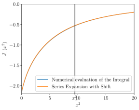
(a) The integral $J_{-}$ for the bosons and $x^{2}\geq 0$.

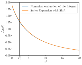
(b) The integral $J_{+}$ for the fermions.

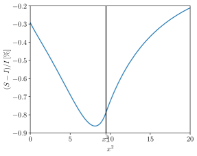
(c) The relative difference in $J_{-}$ for the series expansion ($S$) and the numerical evaluation ($I$).

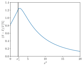
(d) The relative difference in $J_{+}$.

Figure 1: Comparison between the numerical integration and the series expansion of $J_{\pm}(x^{2})$ around $x_{\pm}^{2}$.

In Fig. 1 (upper) we show the series expansion around the transition point $x_{-}^{2}$ ($x_{+}^{2}$) for $J_{-}$ ($J_{+}$) on the left (right) side compared to the numerical evaluation of $J_{-}$ ($J_{+}$). The plots in the lower row show the relative difference between the series expansion $S$ and the numerical evaluation $I$, $(S-I)/I$ in per cent. As can be inferred from Fig. 1 (c), it does not exceed 1% in case of bosons, and for fermions it exceeds $1\%$ only around the transition point, cf. Fig. 1 (d).

2.6 The Minimization of the Effective Potential

For the EWPT to be considered of strong first order, the ratio of the VEV $v_{c}$ at the critical temperature $T_{c}$ has to fulfill $v_{c}/T_{c}>1$. The value $v$ of the VEV at a given temperature $T$ is obtained as

$$v(T)=\left(\sum_{k=1}^{\tilde{n}_{H}}\bar{\omega}_{k}^{2}\right)^{\frac{1}{2}}\;.$$ (2.48)

Here, $\tilde{n}_{H}$ means that the sum is performed over all directions in field space in which we allow for the development of a non-zero electroweak VEV, i.e. the VEV for fields that couple to the EW gauge bosons. We hence do not include here the VEV that a gauge singlet field (as it appears for example in the Next-to-2HDM) develops. The $\bar{\omega}_{k}$ denote the field configurations that minimize the loop-corrected effective potential. Therefore, Eq. (2.48) is the VEV that coincides at $T=0$ with $v=246.22$ GeV. The critical temperature $T_{c}$ is the temperature where two degenerate minima of the potential exist. In order to determine $T_{c}$ the effective potential including the counterterm potential, cf. Eq. (2.4), is minimized numerically at a given temperature $T$. In case of a first order EWPT the VEV jumps from $v=v_{c}$ at the temperature $T_{c}$ to $v=0$ at $T>T_{c}$. For the minimization we use the algorithm CMAES as implemented in libcmaes [26], which finds the global minimum of a given function. As termination criterion we require the relative tolerance of the value of the effective potential between two iterations to be below $10^{-5}$. For the determination of $T_{c}$ we employ a bisection method in the interval $T\in[0,300]\,\mathrm{GeV}$ until the interval containing $T_{c}$ is smaller than $10^{-2}$ GeV. The temperature $T_{c}$ is then set to the lower bound of the final interval. We exclude parameter points for which the individual VEVs obtained from the next-to-leading order (NLO) potential at $T=0$ deviate by more than 1 GeV from their input values as well as parameter points where no PT is found for $T\leq 300$ GeV.

3 Implemented Models

In this section we provide the tree-level potentials as well as the counterterms for the already implemented models. For all implemented models the code expects an input file that presents the input parameters in the same way the program code ScannerS [27, 28] writes them into its default output files. ScannerS is a program that allows to perform extensive scans in the parameter space of multi-Higgs models and checks for compatibility with theoretical and experimental constraints. The viable parameter points can then be fed in our program to investigate the compatibility with a strong first order EWPT e.g.. So far, we have applied our code for such an analysis in the CP-conserving or real 2HDM (R2HDM) [21], the CP-violating or complex 2HDM (C2HDM) [22] and the Next-to-2HDM (N2HDM) [29].

3.1 The CP-Conserving 2HDM

The tree-level Higgs potential of the CP-conserving 2HDM [30, 31] with a softly broken $\mathbb{Z}_{2}$ symmetry, under which the two $SU(2)_{L}$ Higgs doublets $\Phi_{1}$ and $\Phi_{2}$,

$$\Phi_{1}=\begin{pmatrix}\phi_{1}^{+}\\ \phi_{1}^{0}\end{pmatrix}\quad\mbox{and}\quad\Phi_{2}=\begin{pmatrix}\phi_{2}^{+}\\ \phi_{2}^{0}\end{pmatrix}\;,$$ (3.49)

transform as $\Phi_{1}\to\Phi_{1}$, $\Phi_{2}\to-\Phi_{2}$, reads

$$V^{(0)} = m_{11}^{2}\Phi_{1}^{\dagger}\Phi_{1}+m_{22}^{2}\Phi_{2}^{\dagger}\Phi_{2}-m_{12}^{2}\left(\Phi_{1}^{\dagger}\Phi_{2}+h.c.\right)+\frac{\lambda_{1}}{2}\left(\Phi_{1}^{\dagger}\Phi_{1}\right)^{2}+\frac{\lambda_{2}}{2}\left(\Phi_{2}^{\dagger}\Phi_{2}\right)^{2}$$ (3.50)

$$+\lambda_{3}\left(\Phi_{1}^{\dagger}\Phi_{1}\right)\left(\Phi_{2}^{\dagger}\Phi_{2}\right)+\lambda_{4}\left(\Phi_{1}^{\dagger}\Phi_{2}\right)\left(\Phi_{2}^{\dagger}\Phi_{1}\right)+\frac{\lambda_{5}}{2}\left[\left(\Phi_{1}^{\dagger}\Phi_{2}\right)^{2}+h.c.\right]\;.$$

The mass parameters $m_{11}^{2}$, $m_{22}^{2}$ and $m_{12}^{2}$ as well as the quartic couplings $\lambda_{1}...\lambda_{5}$ are real. The parameters $m_{12}^{2}$ and $\lambda_{5}$ can be complex in the CP-violating 2HDM. After EWSB the two Higgs doublets acquire VEVs $\bar{\omega}\in\mathbb{R}$ about which the Higgs fields can be expanded in terms of the charged field components $\rho_{i}$ and $\eta_{i}$ and the neutral CP-even and CP-odd fields $\zeta_{i}$ and $\psi_{i}$ ($i=1,2$),

$$\Phi_{1} = \frac{1}{\sqrt{2}}\begin{pmatrix}\rho_{1}+\mathrm{i}\eta_{1}\\ \zeta_{1}+\bar{\omega}_{1}+\mathrm{i}\psi_{1}\end{pmatrix}$$ (3.51)

$$\Phi_{2} = \frac{1}{\sqrt{2}}\begin{pmatrix}\rho_{2}+\bar{\omega}_{\text{CB}}+\mathrm{i}\eta_{2}\\ \zeta_{2}+\bar{\omega}_{2}+\mathrm{i}\left(\psi_{2}+\bar{\omega}_{\text{CP}}\right)\end{pmatrix}\;.$$ (3.52)

In order to be as general as possible we also allow for CP-violating ($\bar{\omega}_{\text{CP}}$) and charge-breaking ($\bar{\omega}_{\text{CB}}$) VEVs although the latter obviously is unphysical. Note that without loss of generality we have rotated the complex part of the VEVs to the second doublet exclusively. We denote the VEVs of our present vacuum by ($i=1,2,\mbox{CP},\mbox{CB}$)

$$v_{i}\equiv\bar{\omega}_{i}|_{T=0}\;,$$ (3.53)

with

$$v_{\text{CP}}=v_{\text{CB}}=0\;,$$ (3.54)

while the remaining two VEVs are related to the SM VEV $v\approx 246.22$ GeV through

$$v_{1}^{2}+v_{2}^{2}=v^{2}\;.$$ (3.55)

By introducing the angle $\beta$ as

$$\tan\beta=\frac{v_{2}}{v_{1}}\;$$ (3.56)

we have

$$v_{1}=v\cos\beta\quad\mbox{and}\quad v_{2}=v\sin\beta\;.$$ (3.57)

The mixing angle $\beta$ is the rotation angle from the gauge to the mass eigenstates in the charged and in the CP-odd sector, respectively, while we call the mixing angle in the CP-even sector $\alpha$,

$$\left(\begin{array}[]{c}G^{\pm}\\ H^{\pm}\end{array}\right)=R(\beta)\left(\begin{array}[]{c}\phi_{1}^{\pm}\\ \phi_{2}^{\pm}\end{array}\right)\;,\quad\left(\begin{array}[]{c}G^{0}\\ A\end{array}\right)=R(\beta)\left(\begin{array}[]{c}\psi_{1}\\ \psi_{2}\end{array}\right)\;,\quad\left(\begin{array}[]{c}H\\ h\end{array}\right)=R(\alpha)\left(\begin{array}[]{c}\zeta_{1}\\ \zeta_{2}\end{array}\right)\;,$$ (3.70)

with

$$R(x)=\left(\begin{array}[]{cc}\cos x&\sin x\\ -\sin x&\cos x\end{array}\right)\;.$$ (3.73)

We have five physical mass eigenstates, the light and heavy CP-even Higgs bosons $h$ and $H$, the pseudoscalar $A$ and a charged Higgs pair $H^{\pm}$, while $G^{0}$ and $G^{\pm}$ represent the neutral and charged massless Goldstone bosons. The counterterm potential is given as

$$V^{\text{CT}}= \delta m_{11}^{2}\Phi_{1}^{\dagger}\Phi_{1}+\delta m_{22}^{2}\Phi_{2}^{\dagger}\Phi_{2}-\delta m_{12}^{2}\left(\Phi_{1}^{\dagger}\Phi_{2}+\Phi_{2}^{\dagger}\Phi_{1}\right)+\frac{\delta\lambda_{1}}{2}\left(\Phi_{1}^{\dagger}\Phi_{1}\right)^{2}+\frac{\delta\lambda_{2}}{2}\left(\Phi_{2}^{\dagger}\Phi_{2}\right)^{2}$$

$$+\delta\lambda_{3}\left(\Phi_{1}^{\dagger}\Phi_{1}\right)\left(\Phi_{2}^{\dagger}\Phi_{2}\right)+\delta\lambda_{4}\left(\Phi_{1}^{\dagger}\Phi_{2}\right)\left(\Phi_{2}^{\dagger}\Phi_{1}\right)+\frac{\delta\lambda_{5}}{2}\left[\left(\Phi_{1}^{\dagger}\Phi_{2}\right)^{2}+\left(\Phi_{2}^{\dagger}\Phi_{1}\right)^{2}\right]$$

$$+\delta T_{1}\left(\zeta_{1}+\omega_{1}\right)+\delta T_{2}\left(\zeta_{2}+\omega_{2}\right)+\delta T_{\text{CP}}\left(\psi_{2}+\omega_{\text{CP}}\right)+\delta T_{\text{CB}}\left(\rho_{2}+\omega_{\text{CB}}\right)\,.$$ (3.74)

In order to avoid flavour-changing neutral currents (FCNC) at tree level, the $\mathbb{Z}_{2}$ symmetry can also be extended to the Yukawa sector [32, 33]. With four possible $\mathbb{Z}_{2}$ charge assignments there are four different types of 2HDMs as summarized in Table 1.

	$u$-type	$d$-type	leptons
Type I	$\Phi_{2}$	$\Phi_{2}$	$\Phi_{2}$
Type II	$\Phi_{2}$	$\Phi_{1}$	$\Phi_{1}$
Lepton-Specific	$\Phi_{2}$	$\Phi_{2}$	$\Phi_{1}$
Flipped	$\Phi_{2}$	$\Phi_{1}$	$\Phi_{2}$

Table 1: The four Yukawa types of the softly broken $\mathbb{Z}_{2}$-symmetric 2HDM.

The on-shell renormalization that we apply leads to the conditions

$$\left.\partial_{\phi_{i}}V^{\text{CT}}\right|_{\phi=\langle\phi^{c}\rangle_{T=0}} = -\left.\partial_{\phi_{i}}V^{\text{CW}}\right|_{\phi=\langle\phi^{c}\rangle_{T=0}}$$ (3.75)

$$\left.\partial_{\phi_{i}}\partial_{\phi_{j}}V^{\text{CT}}\right|_{\phi=\langle\phi^{c}\rangle_{T=0}} = -\left.\partial_{\phi_{i}}\partial_{\phi_{j}}V^{\text{CW}}\right|_{\phi=\langle\phi^{c}\rangle_{T=0}}\,,$$ (3.76)

where

$$\phi_{i}\equiv\{\rho_{1},\eta_{1},\rho_{2},\eta_{2},\zeta_{1},\psi_{1},\zeta_{2},\psi_{2}\}$$ (3.77)

and $\langle\phi^{c}\rangle_{T=0}$ denotes the field configuration in the minimum at $T=0$,

$$\langle\phi^{c}\rangle_{T=0}=(0,0,0,0,v_{1},0,v_{2},0)\;.$$ (3.78)

These conditions yield the counterterms

$$\delta m_{11}^{2} =\frac{1}{2}H^{\text{CW}}_{\zeta_{1},\zeta_{1}}+H^{\text{CW}}_{\psi_{1},\psi_{1}}-\frac{5}{2}H^{\text{CW}}_{\rho_{1},\rho_{1}}+\frac{1}{2}\frac{v_{2}}{v_{1}}\left(H^{\text{CW}}_{\zeta_{1},\zeta_{2}}-H^{\text{CW}}_{\eta_{1},\eta_{2}}\right)+tv_{2}^{2}$$ (3.79)

$$\delta m_{22}^{2} =\frac{1}{2}\left(H^{\text{CW}}_{\zeta_{2},\zeta_{2}}-3H^{\text{CW}}_{\eta_{2},\eta_{2}}\right)+\frac{1}{2}\frac{v_{1}}{v_{2}}\left(H^{\text{CW}}_{\zeta_{1},\zeta_{2}}-H^{\text{CW}}_{\eta_{1},\eta_{2}}\right)+\frac{v_{1}^{2}}{v_{2}^{2}}\left(H^{\text{CW}}_{\psi_{1},\psi_{1}}-H^{\text{CW}}_{\rho_{1},\rho_{1}}\right)+v_{1}^{2}t$$ (3.80)

$$\delta m_{12}^{2} =H^{\text{CW}}_{\eta_{1},\eta_{2}}+\frac{v_{1}}{v_{2}}\left(H^{\text{CW}}_{\psi_{1},\psi_{1}}-H^{\text{CW}}_{\rho_{1},\rho_{1}}\right)+v_{1}v_{2}t$$ (3.81)

$$\delta\lambda_{1} =\frac{1}{v_{1}^{2}}\left[2H^{\text{CW}}_{\rho_{1},\rho_{1}}-H^{\text{CW}}_{\zeta_{1},\zeta_{1}}-H^{\text{CW}}_{\psi_{1},\psi_{1}}\right]-\frac{v_{2}^{2}}{v_{1}^{2}}t$$ (3.82)

$$\delta\lambda_{2} =\frac{1}{v_{2}^{2}}\left[H^{\text{CW}}_{\eta_{2},\eta_{2}}-H^{\text{CW}}_{\zeta_{2},\zeta_{2}}\right)+\frac{v_{1}^{2}}{v_{2}^{4}}\left(H^{\text{CW}}_{\rho_{1},\rho_{1}}-H^{\text{CW}}_{\psi_{1},\psi_{1}}\right)-\frac{v_{1}^{2}}{v_{2}^{2}}t$$ (3.83)

$$\delta\lambda_{3} =\frac{1}{v_{1}v_{2}}\left(H^{\text{CW}}_{\eta_{1},\eta_{2}}-H^{\text{CW}}_{\zeta_{1},\zeta_{2}}\right)+\frac{1}{v_{2}^{2}}\left(H^{\text{CW}}_{\rho_{1},\rho_{1}}-H^{\text{CW}}_{\psi_{1},\psi_{1}}\right)-t$$ (3.84)

$$\delta\lambda_{4} =t$$ (3.85)

$$\delta\lambda_{5} =\frac{2}{v_{2}^{2}}\left(H^{\text{CW}}_{\psi_{1},\psi_{1}}-H^{\text{CW}}_{\rho_{1},\rho_{1}}\right)+t$$ (3.86)

$$\delta T_{1} =H^{\text{CW}}_{\eta_{1},\eta_{2}}v_{2}+H^{\text{CW}}_{\rho_{1},\rho_{1}}v_{1}-N^{\text{CW}}_{\zeta_{1}}$$ (3.87)

$$\delta T_{2} =H^{\text{CW}}_{\eta_{1},\eta_{2}}v_{1}+H^{\text{CW}}_{\eta_{2},\eta_{2}}v_{2}-N^{\text{CW}}_{\zeta_{2}}$$ (3.88)

$$\delta T_{\text{CP}} =\frac{v_{1}^{2}}{v_{2}}H^{\text{CW}}_{\zeta_{1},\psi_{1}}+H^{\text{CW}}_{\zeta_{1},\psi_{2}}v_{1}-N^{\text{CW}}_{\psi_{2}}$$ (3.89)

$$\delta T_{\text{CB}} =-N^{\text{CW}}_{\rho_{2}}\,,$$ (3.90)

where we used

$$N^{\text{CW}}_{\phi} =\left.\partial_{\phi}V^{\text{CW}}\right|_{\phi=\langle\phi^{c}\rangle_{T=0}}$$ (3.91)

$$H^{\text{CW}}_{\phi_{1},\phi_{2}} =\left.\partial_{\phi_{1}}\partial_{\phi_{2}}V^{\text{CW}}\right|_{\phi_{=}\langle\phi^{c}\rangle_{T=0}}\,.$$ (3.92)

Having less renormalization constants than renormalization conditions, the system of equations is overconstrained. Its consistent solution is given by the following identities

$$0 =H^{\text{CW}}_{\eta_{1},\eta_{1}}-H^{\text{CW}}_{\rho_{1},\rho_{1}}$$ (3.93)

$$0 =H^{\text{CW}}_{\eta_{1},\eta_{2}}-H^{\text{CW}}_{\rho_{1},\rho_{2}}$$ (3.94)

$$0 =H^{\text{CW}}_{\eta_{2},\eta_{2}}-H^{\text{CW}}_{\rho_{2},\rho_{2}}$$ (3.95)

$$0 =H^{\text{CW}}_{\psi_{1},\psi_{2}}-H^{\text{CW}}_{\eta_{1},\eta_{2}}+\frac{v_{1}}{v_{2}}\left(H^{\text{CW}}_{\psi_{1},\psi_{1}}-H^{\text{CW}}_{\rho_{1},\rho_{1}}\right)$$ (3.96)

$$0 =H^{\text{CW}}_{\psi_{2},\psi_{2}}-H^{\text{CW}}_{\eta_{2},\eta_{2}}+\frac{v_{1}^{2}}{v_{2}^{2}}\left(H^{\text{CW}}_{\rho_{1},\rho_{1}}-H^{\text{CW}}_{\psi_{1},\psi_{1}}\right)\,,$$ (3.97)

leading to a one-dimensional solution space parametrized by the parameter $t\in\mathbb{R}$. In the code $t$ is chosen such that

$$\delta\lambda_{4} =0\,.$$ (3.98)

Note that the renormalization constants $\delta T_{\text{CP}}$ and $\delta T_{\text{CB}}$ always turn out to be zero as we do not have CP violation nor charge breaking.

For the eight parameters of the Higgs potential we can either choose a more ’physics’ inspired set involving the masses of the physical Higgs bosons or a pure ’parametric’ input set. The code requires the ’parametric’ input based on $\lambda_{1...5},m_{12}^{2}$ and $\tan\beta$, which has to be given in the order

$$\mbox{type}\;,\;\lambda_{1}\;,\;\lambda_{2}\;,\;\lambda_{3}\;,\;\lambda_{4}\;,\;\lambda_{5}\;,\;m_{12}^{2}\;,\;\tan\beta\;.$$ (3.99)

The user furthermore has to specify through $\mbox{type}=1,...,4$ the type of the 2HDM to be applied, as given in Table 1 where $\mbox{type}=1,...,4$ corresponds to type I, type II, lepton-specific and flipped. Note that the minimum conditions of the potential lead to the following relations among the parameters

$$m_{11}^{2} =m_{12}^{2}\frac{v_{2}}{v_{1}}-\frac{v_{1}^{2}}{2}\lambda_{1}^{2}-\frac{v_{2}^{2}}{2}\left(\lambda_{3}+\lambda_{4}+\lambda_{5}\right)$$ (3.100)

$$m_{22}^{2} =m_{12}^{2}\frac{v_{1}}{v_{2}}-\frac{v_{2}^{2}}{2}\lambda_{2}^{2}-\frac{v_{1}^{2}}{2}\left(\lambda_{3}+\lambda_{4}+\lambda_{5}\right)\,.$$ (3.101)

3.2 The CP-violating 2HDM

Incorporating the softly broken ${\mathbb{Z}}_{2}$ symmetry to avoid FCNC at tree-level (implying the same four different types of 2HDM as in the CP-conserving case, cf. Table 1), the tree-level Higgs potential of the C2HDM [34] reads

$$\begin{split}V^{(0)}&=m_{11}^{2}\Phi_{1}^{\dagger}\Phi_{1}+m_{22}^{2}\Phi_{2}^{\dagger}\Phi_{2}-\left[m_{12}^{2}\Phi_{1}^{\dagger}\Phi_{2}+\mathrm{h.c.}\right]+\frac{1}{2}\lambda_{1}(\Phi_{1}^{\dagger}\Phi_{1})^{2}+\frac{1}{2}\lambda_{2}(\Phi_{2}^{\dagger}\Phi_{2})^{2}\\ &\quad+\lambda_{3}(\Phi_{1}^{\dagger}\Phi_{1})(\Phi_{2}^{\dagger}\Phi_{2})+\lambda_{4}(\Phi_{1}^{\dagger}\Phi_{2})(\Phi_{2}^{\dagger}\Phi_{1})+\left[\frac{1}{2}\lambda_{5}(\Phi_{1}^{\dagger}\Phi_{2})^{2}+\mathrm{h.c.}\right]\;.\end{split}$$ (3.102)

In contrast to the CP-conserving 2HDM, the two parameters $m_{12}^{2}$ and $\lambda_{5}$ can now be complex. If $\mbox{arg}(m_{12}^{2})=\mbox{arg}(\lambda_{5})$ the complex phases of these two parameters can be absorbed by a basis transformation. If additionally the VEVs of the doublets are assumed to be real, we have the real 2HDM. Otherwise, we are in the C2HDM. In the following, we will adopt the conventions of [35]. After EWSB the two Higgs doublets develop VEVs and allowing for the most general vacuum configuration, the expansion about the minimum reads

$$\Phi_{1} = \frac{1}{\sqrt{2}}\begin{pmatrix}\rho_{1}+\mathrm{i}\eta_{1}\\ \zeta_{1}+\bar{\omega}_{1}+\mathrm{i}\psi_{1}\end{pmatrix}$$ (3.103)

$$\Phi_{2} = \frac{1}{\sqrt{2}}\begin{pmatrix}\rho_{2}+\bar{\omega}_{\text{CB}}+\mathrm{i}\eta_{2}\\ \zeta_{2}+\bar{\omega}_{2}+\mathrm{i}\left(\psi_{2}+\bar{\omega}_{\text{CP}}\right)\end{pmatrix}\;.$$ (3.104)

After introducing

$$\zeta_{3}=-\psi_{1}\sin\beta+\psi_{2}\cos\beta$$ (3.105)

the neutral mass eigenstates $H_{i}$ ($i=1,2,3$) are obtained from the C2HDM basis $\zeta_{1},$ $\zeta_{2}$ and $\zeta_{3}$ through the rotation

$$\left(\begin{array}[]{c}H_{1}\\ H_{2}\\ H_{3}\end{array}\right)=R\left(\begin{array}[]{c}\zeta_{1}\\ \zeta_{2}\\ \zeta_{3}\end{array}\right)\;.$$ (3.112)

The mass matrix $R$ can be parametrized in terms of three mixing angles $\alpha_{i}$ ($i=1,2,3$) with $-\pi/2\leq\alpha_{i}<\pi/2$ as

$$R=\left(\begin{array}[]{ccc}c_{1}c_{2}&s_{1}c_{2}&s_{2}\\ -(c_{1}s_{2}s_{3}+s_{1}c_{3})&c_{1}c_{3}-s_{1}s_{2}s_{3}&c_{2}s_{3}\\ -c_{1}s_{2}c_{3}+s_{1}s_{3}&-(c_{1}s_{3}+s_{1}s_{2}c_{3})&c_{2}c_{3}\end{array}\right)\;.$$ (3.116)

All neutral Higgs bosons mix and have no definite CP quantum number. The masses are obtained from the diagonalization of the mass matrix, derived from the Higgs potential, and the conventions are such that $m_{H_{1}}\leq m_{H_{2}}\leq m_{H_{3}}$. The charged sector does not change with respect to the CP-conserving 2HDM, and the mixing angle diagonalizing the charged mixing matrix is given by $\beta$.

The counterterm potential reads

$$V^{\text{CT}}= \delta m_{11}^{2}\Phi_{1}^{\dagger}\Phi_{1}+\delta m_{22}^{2}\Phi_{2}^{\dagger}\Phi_{2}-\left(\delta\mbox{Re}(m_{12}^{2})+\mathrm{i}\delta\mbox{Im}(m_{12}^{2})\right)\Phi_{1}^{\dagger}\Phi_{2}-\left(\delta\mbox{Re}(m_{12}^{2})-\mathrm{i}\delta\mbox{Im}(m_{12}^{2})\right)\Phi_{2}^{\dagger}\Phi_{1}$$

$$+\frac{\delta\lambda_{1}}{2}\left(\Phi_{1}^{\dagger}\Phi_{1}\right)^{2}+\frac{\delta\lambda_{2}}{2}\left(\Phi_{2}^{\dagger}\Phi_{2}\right)^{2}+\delta\lambda_{3}\left(\Phi_{1}^{\dagger}\Phi_{1}\right)\left(\Phi_{2}^{\dagger}\Phi_{2}\right)+\delta\lambda_{4}\left(\Phi_{1}^{\dagger}\Phi_{2}\right)\left(\Phi_{2}^{\dagger}\Phi_{1}\right)$$

$$+\frac{1}{2}\left(\delta\mbox{Re}(\lambda_{5})+\mathrm{i}\delta\mbox{Im}(\lambda_{5})\right)\left(\Phi_{1}^{\dagger}\Phi_{2}\right)^{2}+\frac{1}{2}\left(\delta\mbox{Re}(\lambda_{5})-\mathrm{i}\delta\mbox{Im}(\lambda_{5})\right)\left(\Phi_{2}^{\dagger}\Phi_{1}\right)^{2}$$

$$+\delta T_{1}\left(\zeta_{1}+\omega_{1}\right)+\delta T_{2}\left(\zeta_{2}+\omega_{2}\right)+\delta T_{\text{CP}}\left(\psi_{2}+\omega_{\text{CP}}\right)+\delta T_{\text{CB}}\left(\rho_{2}+\omega_{\text{CB}}\right)\,.$$ (3.117)

Using

$$\phi_{i}\equiv\{\rho_{1},\eta_{1},\rho_{2},\eta_{2},\zeta_{1},\psi_{1},\zeta_{2},\psi_{2}\}$$ (3.118)

the ’on-shell’ renormalization conditions yield

$$\left.\partial_{\phi_{i}}V^{\text{CT}}\right|_{\phi=\langle\phi^{c}\rangle_{T=0}} = -\left.\partial_{\phi_{i}}V^{\text{CW}}\right|_{\phi=\langle\phi^{c}\rangle_{T=0}}$$ (3.119)

$$\left.\partial_{\phi_{i}}\partial_{\phi_{j}}V^{\text{CT}}\right|_{\phi=\langle\phi^{c}\rangle_{T=0}} = -\left.\partial_{\phi_{i}}\partial_{\phi_{j}}V^{\text{CW}}\right|_{\phi=\langle\phi^{c}\rangle_{T=0}}\,,$$ (3.120)

with

$$\langle\phi^{c}\rangle_{T=0}=(0,0,0,0,v_{1},0,v_{2},0)\;,$$ (3.121)

and lead to the counterterms

$$\delta m_{11}^{2} =\frac{1}{2}\left[H^{\text{CW}}_{\zeta_{1},\zeta_{1}}-2H^{\text{CW}}_{\psi_{1},\psi_{1}}-H^{\text{CW}}_{\eta_{1},\eta_{2}}\frac{v_{2}}{v_{1}}+H^{\text{CW}}_{\zeta_{1},\zeta_{2}}\frac{v_{2}}{v_{1}}-H^{\text{CW}}_{\rho_{1},\rho_{1}}\right]+v_{2}^{2}t$$ (3.122)

$$\delta m_{22}^{2} =\left[-\frac{1}{2}\frac{v_{1}}{v_{2}}\left(H^{\text{CW}}_{\eta_{1},\eta_{2}}-H^{\text{CW}}_{\zeta_{1},\zeta_{2}}\right)+\frac{v_{1}^{2}}{v_{2}^{2}}\left(H^{\text{CW}}_{\rho_{1},\rho_{1}}-H^{\text{CW}}_{\psi_{1},\psi_{1}}\right)-\frac{3}{2}H^{\text{CW}}_{\eta_{2},\eta_{2}}+\frac{1}{2}H^{\text{CW}}_{\zeta_{2},\zeta_{2}}\right]+v_{1}^{2}t$$ (3.123)

$$\delta\text{Re}\!\,(m_{12}^{2}) =\left[H^{\text{CW}}_{\eta_{1},\eta_{2}}-\frac{v_{1}}{v_{2}}H^{\text{CW}}_{\psi_{1},\psi_{1}}+\frac{v_{1}}{v_{2}}H^{\text{CW}}_{\rho_{1},\rho_{1}}\right]+v_{1}v_{2}t$$ (3.124)

$$\delta\lambda_{1} =\frac{1}{v_{1}^{2}}\left[H^{\text{CW}}_{\psi_{1},\psi_{1}}-H^{\text{CW}}_{\zeta_{1},\zeta_{1}}\right]-\frac{v_{2}^{2}}{v_{1}^{2}}t$$ (3.125)

$$\delta\lambda_{2} =\frac{1}{v_{2}^{2}}\left[H^{\text{CW}}_{\eta_{2},\eta_{2}}-H^{\text{CW}}_{\zeta_{2},\zeta_{2}}+\frac{v_{1}^{2}}{v_{2}^{2}}\left(H^{\text{CW}}_{\psi_{1},\psi_{1}}-H^{\text{CW}}_{\rho_{1},\rho_{1}}\right)\right]-\frac{v_{1}^{2}}{v_{2}^{2}}t$$ (3.126)

$$\delta\lambda_{3} =\frac{1}{v_{1}v_{2}}\left[H^{\text{CW}}_{\eta_{1},\eta_{2}}-H^{\text{CW}}_{\zeta_{1},\zeta_{2}}+\frac{v_{1}}{v_{2}}\left(H^{\text{CW}}_{\psi_{1},\psi_{1}}-H^{\text{CW}}_{\rho_{1},\rho_{1}}\right)\right]-t$$ (3.127)

$$\delta\lambda_{4} =\frac{2}{v_{2}^{2}}\left[H^{\text{CW}}_{\rho_{1},\rho_{1}}-H^{\text{CW}}_{\psi_{1},\psi_{1}}\right]+t$$ (3.128)

$$\delta\text{Re}\!\,(\lambda_{5}) =t$$ (3.129)

$$\delta\text{Im}\!\,(\lambda_{5}) =-\frac{2}{v_{2}^{2}}H^{\text{CW}}_{\zeta_{1},\psi_{1}}$$ (3.130)

$$\delta\text{Im}\!\,(m_{12}^{2}) =-\left[H^{\text{CW}}_{\zeta_{1},\psi_{2}}+2\frac{v_{1}}{v_{2}}H^{\text{CW}}_{\zeta_{1},\psi_{1}}\right]$$ (3.131)

$$\delta T_{1} =H^{\text{CW}}_{\eta_{1},\eta_{2}}v_{2}+H^{\text{CW}}_{\rho_{1},\rho_{1}}v_{1}-N^{\text{CW}}_{\zeta_{1}}$$ (3.132)

$$\delta T_{2} =H^{\text{CW}}_{\eta_{1},\eta_{2}}v_{1}+H^{\text{CW}}_{\eta_{2},\eta_{2}}v_{2}-N^{\text{CW}}_{\zeta_{2}}$$ (3.133)

$$\delta T_{\text{CP}} =\frac{v_{1}^{2}}{v_{2}}H^{\text{CW}}_{\zeta_{1},\psi_{1}}+H^{\text{CW}}_{\zeta_{1},\psi_{2}}v_{1}-N^{\text{CW}}_{\psi_{2}}$$ (3.134)

$$\delta T_{\text{CB}} =-N^{\text{CW}}_{\rho_{2}}\;,$$ (3.135)

where we used the abbreviations Eqs. (3.91) and (3.92). Again, the system of equations is overconstrained. Its one-dimensional solution space is parametrized by $t\in\mathbb{R}$ which we have chosen such that

$$\delta\lambda_{4} =0\,.$$ (3.136)

With this choice Eqs. (3.122)–(3.129) simplify to

$$\delta m_{11}^{2} =\frac{1}{2}\left[H_{\zeta_{1},\zeta_{1}}^{\text{CW}}+2H_{\psi_{1},\psi_{1}}^{\text{CW}}-\frac{v_{2}}{v_{1}}\left(H^{\text{CW}}_{\eta_{1},\eta_{2}}-H^{\text{CW}}_{\zeta_{1},\zeta_{2}}\right)-5H^{\text{CW}}_{\rho_{1},\rho 1}\right]$$ (3.137)

$$\delta m_{22}^{2} =\frac{1}{2}\left[\frac{v_{1}}{v_{2}}\left(H^{\text{CW}}_{\zeta_{1},\zeta_{2}}-H^{\text{CW}}_{\eta_{1},\eta_{2}}\right)-\frac{v_{1}^{2}}{v_{2}^{2}}\left(H^{\text{CW}}_{\rho_{1},\rho_{1}}-H^{\text{CW}}_{\psi_{1},\psi_{1}}\right)-3H^{\text{CW}}_{\eta_{2},\eta_{2}}+H^{\text{CW}}_{\zeta_{2},\zeta_{2}}\right]$$ (3.138)

$$\delta\text{Re}\!\,(m_{12}^{2}) =\frac{v_{1}}{v_{2}}\left(H^{\text{CW}}_{\psi_{1},\psi_{1}}-H^{\text{CW}}_{\rho_{1},\rho_{1}}\right)+H^{\text{CW}}_{\eta_{1},\eta_{2}}$$ (3.139)

$$\delta\lambda_{1} =\frac{1}{v_{1}^{2}}\left(2H^{\text{CW}}_{\rho_{1},\rho_{1}}-H^{\text{CW}}_{\psi_{1},\psi_{1}}-H^{\text{CW}}_{\zeta_{1},\zeta_{1}}\right)$$ (3.140)

$$\delta\lambda_{2} =\frac{1}{v_{2}^{2}}\left[\frac{v_{1}^{2}}{v_{2}^{2}}\left(H^{\text{CW}}_{\rho_{1},\rho_{1}}-H^{\text{CW}}_{\psi_{1},\psi_{1}}\right)+H^{\text{CW}}_{\eta_{2},\eta_{2}}-H^{\text{CW}}_{\zeta_{2},\zeta_{2}}\right]$$ (3.141)

$$\delta\lambda_{3} =\frac{1}{v_{1}v_{2}^{2}}\left[\left(H^{\text{CW}}_{\rho_{1},\rho_{1}}-H^{\text{CW}}_{\psi_{1},\psi_{1}}\right)v_{1}+\left(H^{\text{CW}}_{\eta_{1},\eta_{2}}-H^{\text{CW}}_{\zeta_{1},\zeta_{2}}\right)v_{2}\right]$$ (3.142)

$$\delta\lambda_{4} =0$$ (3.143)

$$\delta\text{Re}\!\,(\lambda_{5}) =\frac{2}{v_{2}^{2}}\left(H^{\text{CW}}_{\psi_{1},\psi_{1}}-H^{\text{CW}}_{\rho_{1},\rho_{1}}\right)\;,$$ (3.144)

where we have applied the identities needed for the consistent solution,

$$0 =H^{\text{CW}}_{\eta_{1},\eta_{1}}-H^{\text{CW}}_{\rho_{1},\rho_{1}}$$ (3.145)

$$0 =H^{\text{CW}}_{\eta_{1},\eta_{2}}-H^{\text{CW}}_{\rho_{1},\rho_{2}}$$ (3.146)

$$0 =H^{\text{CW}}_{\eta_{2},\eta_{2}}-H^{\text{CW}}_{\rho_{2},\rho_{2}}$$ (3.147)

$$0 =H^{\text{CW}}_{\psi_{1},\psi_{2}}-H^{\text{CW}}_{\eta_{1},\eta_{2}}+\frac{v_{1}}{v_{2}}\left(H^{\text{CW}}_{\psi_{1},\psi_{1}}-H^{\text{CW}}_{\rho_{1},\rho_{1}}\right)$$ (3.148)

$$0 =H^{\text{CW}}_{\psi_{2},\psi_{2}}-H^{\text{CW}}_{\eta_{2},\eta_{2}}+\frac{v_{1}^{2}}{v_{2}^{2}}\left(H^{\text{CW}}_{\rho_{1},\rho_{1}}-H^{\text{CW}}_{\psi_{1},\psi_{1}}\right)$$ (3.149)

$$0 =H^{\text{CW}}_{\zeta_{1},\psi_{2}}v_{2}+v_{1}H^{\text{CW}}_{\zeta_{1},\psi_{1}}v_{1}+N^{\text{CW}}_{\psi_{1}}$$ (3.150)

$$0 =H^{\text{CW}}_{\rho_{1},\eta_{2}}-H^{\text{CW}}_{\zeta_{1},\psi_{2}}-\frac{v_{1}}{v_{2}}H^{\text{CW}}_{\zeta_{1},\psi_{1}}$$ (3.151)

$$0 =H^{\text{CW}}_{\zeta_{1},\psi_{2}}+H^{\text{CW}}_{\eta_{1},\rho_{2}}+\frac{v_{1}}{v_{2}}H^{\text{CW}}_{\zeta_{1},\psi_{1}}$$ (3.152)

$$0 =H^{\text{CW}}_{\psi_{1},\zeta_{2}}+H^{\text{CW}}_{\zeta_{1},\psi_{2}}$$ (3.153)

$$0 =\frac{v_{1}^{2}}{v_{2}^{2}}H^{\text{CW}}_{\zeta_{1},\psi_{1}}+H^{\text{CW}}_{\zeta_{2},\psi_{2}}\;.$$ (3.154)

Note that $\delta T_{\text{CB}}$ related to the charge breaking VEV turns out to be zero as we do not have a charge-breaking vacuum.

The C2HDM is parametrized by nine independent parameters. In a physics-inspired basis the masses are part of the input, in the ’parametric’ basis, used in the code, the input parameters in addition to the SM VEV hard-coded in the program, are, in the order required by the program,

$$\mbox{type}\;,\;\lambda_{1}\;,\;\lambda_{2}\;,\;\lambda_{3}\;,\;\lambda_{4}\;,\;\mbox{Re}\lambda_{5}\;,\;\mbox{Im}(\lambda_{5})\;,\;\mbox{Re}(m_{12}^{2})\;,\;\tan\beta\;.$$ (3.155)

By setting $\mbox{type}=1,2,3$ or 4, the user chooses the C2HDM type. The parameters $m_{11}^{2},m_{22}^{2}$ and $\mbox{Im}(m_{12}^{2})$ are obtained from the minimum conditions

$$m_{11}^{2} =\mbox{Re}(m_{12}^{2})\frac{v_{2}}{v_{1}}-\frac{v_{1}^{2}}{2}\lambda_{1}^{2}-\frac{v_{2}^{2}}{2}\left(\lambda_{3}+\lambda_{4}+\mbox{Re}(\lambda_{5})\right)$$ (3.156)

$$m_{22}^{2} =\mbox{Re}(m_{12}^{2})\frac{v_{1}}{v_{2}}-\frac{v_{2}^{2}}{2}\lambda_{2}^{2}-\frac{v_{1}^{2}}{2}\left(\lambda_{3}+\lambda_{4}+\mbox{Re}(\lambda_{5})\right)$$ (3.157)

$$\mbox{Im}(m_{12}^{2}) =\frac{v_{1}v_{2}}{2}\mbox{Im}(\lambda_{5})\,.$$ (3.158)

3.3 The N2HDM

The N2HDM is built from the CP-conserving 2HDM with a softly broken $\mathbb{Z}_{2}$ symmetry upon extension by a singlet field $\Phi_{S}$. If the latter does not acquire a VEV, we have a dark matter candidate [38]. Here, we let the singlet field have a non-vanishing VEV. (For the phenomenology of the N2HDM with a singlet VEV, see [39] with and [37, 40] without any approximations. The NLO electroweak corrected N2HDM and in particular its renormalization has been presented in [41].) The tree-level potential of the N2HDM is given by

$$V^{(0)} = m_{11}^{2}\Phi_{1}^{\dagger}\Phi_{1}+m_{22}^{2}\Phi_{2}^{\dagger}\Phi_{2}-m_{12}^{2}\left(\Phi_{1}^{\dagger}\Phi_{2}+\Phi_{2}^{\dagger}\Phi_{1}\right)+\frac{\lambda_{1}}{2}\left(\Phi_{1}^{\dagger}\Phi_{1}\right)^{2}+\frac{\lambda_{2}}{2}\left(\Phi_{2}^{\dagger}\Phi_{2}\right)^{2}$$ (3.159)

$$+\lambda_{3}\left(\Phi_{1}^{\dagger}\Phi_{1}\right)\left(\Phi_{2}^{\dagger}\Phi_{2}\right)+\lambda_{4}\left(\Phi_{1}^{\dagger}\Phi_{2}\right)\left(\Phi_{2}^{\dagger}\Phi_{1}\right)+\frac{\lambda_{5}}{2}\left[\left(\Phi_{1}^{\dagger}\Phi_{2}\right)^{2}+\left(\Phi_{2}^{\dagger}\Phi_{1}\right)^{2}\right]$$

$$+\frac{1}{2}m_{S}^{2}\Phi_{S}^{2}+\frac{\lambda_{6}}{8}\Phi_{S}^{4}+\frac{\lambda_{7}}{2}\left(\Phi_{1}^{\dagger}\Phi_{1}\right)\Phi_{S}^{2}+\frac{\lambda_{8}}{2}\left(\Phi_{2}^{\dagger}\Phi_{2}\right)\Phi_{S}^{2}\;,$$

where the first two lines describe the 2HDM part of the N2HDM and the last line is the contribution of the singlet field $\Phi_{S}$. The potential obeys two $\mathbb{Z}_{2}$ symmetries. The first one, named $\mathbb{Z}_{2}$, is the trivial generalization of the usual 2HDM $\mathbb{Z}_{2}$ symmetry to the N2HDM,

$$\Phi_{1}\to\Phi_{1}\;,\quad\Phi_{2}\to-\Phi_{2}\;,\quad\Phi_{S}\to\Phi_{S}\;,$$ (3.160)

and is softly broken by the term proportional to $m_{12}^{2}$. Its extension to the Yukawa sector ensures the absence of FCNC and implies different types of N2HDM that are the same as in the 2HDM, summarized in Table 1. The second one, named $\mathbb{Z}_{2}^{\prime}$, is given by

$$\Phi_{1}\to\Phi_{1}\;,\quad\Phi_{2}\to\Phi_{2}\;,\quad\Phi_{S}\to-\Phi_{S}\;,$$ (3.161)

and is not explicitly broken. For a non-vanishing VEV of $\Phi_{S}$ as allowed here, there is mixing among all CP-even neutral scalars. This is also the case if $m_{12}^{2}=0$, which will not be considered here, however. After EWSB, the doublets and the singlet field acquire VEVs about which they can be expanded as (allowing for the most general vacuum configuration with CP- and (unphysical) CB-violating VEVs),

$$\Phi_{1} = \frac{1}{\sqrt{2}}\begin{pmatrix}\rho_{1}+\mathrm{i}\eta_{1}\\ \zeta_{1}+\bar{\omega}_{1}+\mathrm{i}\psi_{1}\end{pmatrix}$$ (3.162)

$$\Phi_{2} = \frac{1}{\sqrt{2}}\begin{pmatrix}\rho_{2}+\bar{\omega}_{\text{CB}}+\mathrm{i}\eta_{2}\\ \zeta_{2}+\bar{\omega}_{2}+\mathrm{i}\left(\psi_{2}+\bar{\omega}_{\text{CP}}\right)\end{pmatrix}$$ (3.163)

$$\Phi_{S} = \bar{\omega}_{S}+\rho_{S}\;.$$ (3.164)

The diagonalization of the mass matrix of the neutral scalar fields, obtained after EWSB from the second derivative of the potential with respect to these fields, leads to three neutral physical Higgs states, $H_{1}$, $H_{2}$ and $H_{3}$ that are ordered by ascending mass, i.e. $m_{H_{1}}\leq m_{H_{2}}\leq m_{H_{3}}$. The CP-odd and the charged sector do not change with respect to the real 2HDM, and we have a pseudoscalar Higgs $A$ and two charged Higgs states $H^{\pm}$. The N2HDM counterterm potential reads

$$V^{\text{CT}} = \delta m_{11}^{2}\Phi_{1}^{\dagger}\Phi_{1}+\delta m_{22}^{2}\Phi_{2}^{\dagger}\Phi_{2}-\delta m_{12}^{2}\left(\Phi_{1}^{\dagger}\Phi_{2}+\Phi_{2}^{\dagger}\Phi_{1}\right)+\frac{\delta\lambda_{1}}{2}\left(\Phi_{1}^{\dagger}\Phi_{1}\right)^{2}+\frac{\delta\lambda_{2}}{2}\left(\Phi_{2}^{\dagger}\Phi_{2}\right)^{2}$$ (3.165)

$$+\delta\lambda_{3}\left(\Phi_{1}^{\dagger}\Phi_{1}\right)\left(\Phi_{2}^{\dagger}\Phi_{2}\right)+\delta\lambda_{4}\left(\Phi_{1}^{\dagger}\Phi_{2}\right)\left(\Phi_{2}^{\dagger}\Phi_{1}\right)+\frac{\delta\lambda_{5}}{2}\left[\left(\Phi_{1}^{\dagger}\Phi_{2}\right)^{2}+\left(\Phi_{2}^{\dagger}\Phi_{1}\right)^{2}\right]$$

$$+\frac{1}{2}\delta m_{S}^{2}\Phi_{S}^{2}+\frac{\delta\lambda_{6}}{8}\Phi_{S}^{4}+\frac{\delta\lambda_{7}}{2}\left(\Phi_{1}^{\dagger}\Phi_{1}\right)\Phi_{S}^{2}+\frac{\delta\lambda_{8}}{2}\left(\Phi_{2}^{\dagger}\Phi_{2}\right)\Phi_{S}^{2}$$

$$+\delta T_{1}(\zeta_{1}+\omega_{1})+\delta T_{2}(\zeta_{2}+\omega_{2})+\delta T_{\text{CP}}(\psi_{2}+\omega_{\text{CP}})$$

$$+\delta T_{\text{CB}}(\rho_{2}+\omega_{\text{CB}})+\delta T_{S}(\rho_{S}+\omega_{S})\;.$$

Using

$$\phi_{i}\equiv\{\rho_{1},\eta_{1},\rho_{2},\eta_{2},\zeta_{1},\psi_{1},\zeta_{2},\psi_{2},\rho_{S}\}$$ (3.166)

the ’on-shell’ renormalization conditions yield

$$\left.\partial_{\phi_{i}}V^{\text{CT}}\right|_{\phi=\langle\phi^{c}\rangle_{T=0}} = -\left.\partial_{\phi_{i}}V^{\text{CW}}\right|_{\phi=\langle\phi^{c}\rangle_{T=0}}$$ (3.167)

$$\left.\partial_{\phi_{i}}\partial_{\phi_{j}}V^{\text{CT}}\right|_{\phi=\langle\phi^{c}\rangle_{T=0}} = -\left.\partial_{\phi_{i}}\partial_{\phi_{j}}V^{\text{CW}}\right|_{\phi=\langle\phi^{c}\rangle_{T=0}}\,,$$ (3.168)

with

$$\langle\phi^{c}\rangle_{T=0}=(0,0,0,0,v_{1},0,v_{2},0,v_{S})\;,$$ (3.169)

and lead to the counterterms

$$\delta m_{11}^{2}= \frac{1}{2}\left[\frac{v_{s}}{v_{1}}H^{\text{CW}}_{\rho_{1},\rho_{S}}+\frac{v_{2}}{v_{1}}\left(H^{\text{CW}}_{\rho_{1},\rho_{2}}-H^{\text{CW}}_{\psi_{1},\psi_{2}}\right)+2H^{\text{CW}}_{\psi_{1},\psi_{1}}-5H^{\text{CW}}_{\psi_{1},\psi_{1}}+H^{\text{CW}}_{\rho_{1},\rho_{1}}\right]+t_{H}v_{2}^{2}$$ (3.170)

$$\delta m_{22}^{2}= \frac{1}{2}\left[\frac{v_{s}}{v_{2}}H^{\text{CW}}_{\rho_{2},\rho_{S}}+H^{\text{CW}}_{\rho_{2},\rho_{2}}-3H^{\text{CW}}_{\psi_{2},\psi_{2}}+\frac{v_{1}}{v_{2}}\left(H^{\text{CW}}_{\rho_{1},\rho_{2}}-H^{\text{CW}}_{\psi_{1},\psi_{2}}\right)+5\frac{v_{1}^{2}}{v_{2}^{2}}\left(H^{\text{CW}}_{\psi_{1},\psi_{1}}-H^{\text{CW}}_{\psi_{1},\psi_{1}}\right)\right]+t_{H}v_{1}^{2}$$ (3.171)

$$\delta m_{12}^{2} =H^{\text{CW}}_{\psi_{1},\psi_{2}}+\frac{v_{1}}{v_{2}}\left(H^{\text{CW}}_{\psi_{1},\psi_{1}}-H^{\text{CW}}_{\psi_{1},\psi_{1}}\right)+t_{H}v_{1}v_{2}$$ (3.172)

$$\delta\lambda_{1} =\frac{1}{v_{1}^{2}}\left(2H^{\text{CW}}_{\psi_{1},\psi_{1}}-H^{\text{CW}}_{\psi_{1},\psi_{1}}-H^{\text{CW}}_{\rho_{1},\rho_{1}}\right)-t_{H}\frac{v_{2}^{2}}{v_{1}^{2}}$$ (3.173)

$$\delta\lambda_{2} =\frac{1}{v_{2}^{2}}\left(H^{\text{CW}}_{\psi_{2},\psi_{2}}-H^{\text{CW}}_{\rho_{2},\rho_{2}}\right)+2\frac{v_{1}^{2}}{v_{2}^{4}}\left(H^{\text{CW}}_{\psi_{1},\psi_{1}}-H^{\text{CW}}_{\psi_{1},\psi_{1}}\right)-t_{H}\frac{v_{1}^{2}}{v_{2}^{2}}$$ (3.174)

$$\delta\lambda_{3} =\frac{1}{v_{2}^{2}}\left(H^{\text{CW}}_{\psi_{1},\psi_{1}}-H^{\text{CW}}_{\psi_{1},\psi_{1}}\right)+\frac{1}{v_{1}v_{2}}\left(H^{\text{CW}}_{\psi_{1},\psi_{2}}-H^{\text{CW}}_{\rho_{1},\rho_{2}}\right)-t_{H}$$ (3.175)

$$\delta\lambda_{4} =t_{H}$$ (3.176)

$$\delta\lambda_{5} =\frac{2}{v_{2}^{2}}\left(H^{\text{CW}}_{\psi_{1},\psi_{1}}-2H^{\text{CW}}_{\psi_{1},\psi_{1}}\right)+t_{H}$$ (3.177)

$$\delta m_{S}^{2} =\frac{1}{2}\left(H^{\text{CW}}_{\rho_{S},\rho_{S}}+\frac{v_{2}}{v_{s}}H^{\text{CW}}_{\rho_{2},\rho_{S}}+\frac{v_{1}}{v_{s}}H^{\text{CW}}_{\rho_{1},\rho_{S}}-\frac{3}{v_{S}}N^{\text{CW}}_{\rho_{S}}\right)-t_{S}\frac{3}{2v_{s}}$$ (3.178)

$$\delta\lambda_{6} =\frac{1}{v_{s}^{3}}\left(N^{\text{CW}}_{\rho_{S}}-v_{s}H^{\text{CW}}_{\rho_{S},\rho_{S}}\right)-t_{S}\frac{1}{v_{s}^{3}}$$ (3.179)

$$\delta\lambda_{7} =-\frac{1}{v_{s}v_{1}}H^{\text{CW}}_{\rho_{1},\rho_{S}}$$ (3.180)

$$\delta\lambda_{8} =-\frac{1}{v_{s}v_{2}}H^{\text{CW}}_{\rho_{2},\rho_{S}}$$ (3.181)

$$\delta T_{1} =H^{\text{CW}}_{\psi_{1},\psi_{1}}v_{1}+H^{\text{CW}}_{\psi_{1},\psi_{2}}v_{2}-N^{\text{CW}}_{\rho_{1}}$$ (3.182)

$$\delta T_{2} =\frac{v_{1}^{2}}{v_{2}}\left(H^{\text{CW}}_{\psi_{1},\psi_{1}}-H^{\text{CW}}_{\psi_{1},\psi_{1}}\right)+H^{\text{CW}}_{\psi_{1},\psi_{2}}v_{1}+H_{\psi_{2},\psi_{2}}v_{2}-N^{\text{CW}}_{\zeta_{2}}$$ (3.183)

$$\delta T_{S} =t_{S}$$ (3.184)

$$\delta T_{\text{CP}} =\frac{v_{1}^{2}}{v_{2}}H^{\text{CW}}_{\rho_{1},\psi_{1}}+H^{\text{CW}}_{\rho_{1},\psi_{2}}v_{1}-N^{\text{CW}}_{\psi_{2}}$$ (3.185)

$$\delta T_{\text{CB}} =-N^{\text{CW}}_{\zeta_{2}}\;,$$ (3.186)

where we used the abbreviations Eqs. (3.91) and (3.92). The overconstrained system of equations leads to a two-dimensional solution space parametrized by $t_{H},t_{S}\in\mathbb{R}$ that we set in the code to

$$t_{H}=t_{S}=0\;.$$ (3.187)

The identities to be applied to solve the system of equations are the same as in the R2HDM and given by

$$0 =H^{\text{CW}}_{\eta_{1},\eta_{1}}-H^{\text{CW}}_{\rho_{1},\rho_{1}}$$ (3.188)

$$0 =H^{\text{CW}}_{\eta_{1},\eta_{2}}-H^{\text{CW}}_{\rho_{1},\rho_{2}}$$ (3.189)

$$0 =H^{\text{CW}}_{\eta_{2},\eta_{2}}-H^{\text{CW}}_{\rho_{2},\rho_{2}}$$ (3.190)

$$0 =H^{\text{CW}}_{\psi_{1},\psi_{2}}-H^{\text{CW}}_{\eta_{1},\eta_{2}}+\frac{v_{1}}{v_{2}}\left(H^{\text{CW}}_{\psi_{1},\psi_{1}}-H^{\text{CW}}_{\rho_{1},\rho_{1}}\right)$$ (3.191)

$$0 =H^{\text{CW}}_{\psi_{2},\psi_{2}}-H^{\text{CW}}_{\eta_{2},\eta_{2}}+\frac{v_{1}^{2}}{v_{2}^{2}}\left(H^{\text{CW}}_{\rho_{1},\rho_{1}}-H^{\text{CW}}_{\psi_{1},\psi_{1}}\right)\,.$$ (3.192)

As a charge-breaking vacuum is unphysical, $\delta T_{\text{CB}}$ always turns out to be zero as it should. The program code requires (in addition to the SM VEV that is hard-coded) the ’parametric’ input parameters for the N2HDM to be given in the order

$$\mbox{type}\;,\;\lambda_{1}\;,\;\lambda_{2}\;,\;\lambda_{3}\;,\;\lambda_{4}\;,\;\lambda_{5}\;,\;\lambda_{6}\;,\;\lambda_{7}\;,\;\lambda_{8}\;,\;v_{S}\;,\;\tan\beta\;,\;m_{12}^{2}\;.$$ (3.193)

In the first entry, the user has to specify the N2HDM type. Note that the minimum conditions lead to the following relations among the parameters

$$\frac{v_{2}}{v_{1}}m_{12}^{2}-m_{11}^{2} = \frac{1}{2}(v_{1}^{2}\lambda_{1}+v_{2}^{2}\lambda_{345}+v_{S}^{2}\lambda_{7})$$ (3.194)

$$\frac{v_{1}}{v_{2}}m_{12}^{2}-m_{22}^{2} = \frac{1}{2}(v_{1}^{2}\lambda_{345}+v_{2}^{2}\lambda_{2}+v_{S}^{2}\lambda_{8})$$ (3.195)

$$-m_{S}^{2} = \frac{1}{2}(v_{1}^{2}\lambda_{7}+v_{2}^{2}\lambda_{8}+v_{S}^{2}\lambda_{6})\;,$$ (3.196)

with

$$\lambda_{345}\equiv\lambda_{3}+\lambda_{4}+\lambda_{5}\;.$$ (3.197)

4 Installation

Download

The program can be downloaded from https://github.com/phbasler/BSMPT . After extracting the zip archive in the directory chosen by the user, to which we will from now on refer as $BSMPT, there will be several subfolders. These are:

docs	The docs folder contains the documentation as html.
example	Here we put sample input files as well as the corresponding results produced
	by the different executables (see below).
manual	This subfolder contains a copy of this paper which is kept up to date
	with changes in the code. Additionally, we include the changelog
	file documenting corrected bugs and modifications of the program.
sh	Here we put the script to install the libraries and to create the makefile. Here
	we also provide the python files prepareData_XXX.py (XXX= R2HDM,
	C2HDM, N2HDM) that can be used to order the data sample accordingly to
	the input requirements.
src	This subfolder contains the source files of the code and is structured in three
	subfolders.

The subfolders of src contain the following files:

src/minimizer	Here the source files for the minimization routines are stored.
src/models	This directory contains the implemented models.
	If a new model is added it must be placed in this folder.
	There is also a template class with instructions on how
	to add a new model. Furthermore, there is the file
	SMparam.h with the Standard Model parameters.
src/prog	This directory contains the source code for the executables.

Required libraries

For BSMPT to work the following three libraries are needed:

• The GNU Scientific Library (GSL) [42] is assumed to be installed in PATH. GSL is required for the calculation of the Riemann-$\zeta$ functions, the double factorial and for the minimization.

• The Eigen3 library [43] is downloaded during the installation process of BSMPT. Eigen3 is used for all the matrix calculations.

• The libcmaes library [26] is required for the minimization and is installed during the installation process.

Compilation

The compilation requires a C++ and C compiler that support the C++11 standard. For the C++ compiler we recommend g++-7 and for the C compiler we recommend gcc-7. After that, the following steps have to be performed:

1. Go to the folder $BSMPT/sh and call
          

   ./InstallLibraries.sh –lib=PathToYourLib –CXX=C++Compiler –CC=CCompiler

   
   where ’PathToYourLib’, is the absolute path in which Eigen3 and libcmaes will be installed by this script.

2. To generate the Makefile in the $BSMPT  folder call
          

   ./autogen.sh –lib=PathToYourLib –CXX=C++Compiler

3. Go back to $BSMPT  and call
          

   make

   
   which will generate the executables BSMPT, CalcCT, NLOVEV, TripleHiggsNLO and VEVEVO.

After that go to the folder PathToYourLib/libcmaes and check if there is either the folder lib or lib64. Then
       

export LD_LIBRARY_PATH=$LD_LIBRARY_PATH:PathToYourLib/libcmaes/LIB

has to be executed where ’LIB’ is either lib64 or lib, depending on which folder exists in PathToYourLib/libcmaes. This can also be added to bashrc so that it is loaded automatically with every new terminal that is opened.

5 Executables

In this section we will briefly describe the executables that are generated by the makefile. We begin with the definition of the input parameters that are used by all executables:

• Model is the parameter by which the model is selected. The CP-violating 2HDM (0), the CP-conserving 2HDM (1) and the CP-conserving N2HDM (2), as introduced in Section 3, are already implemented.

• Inputfile sets the path and the name of the input file. In the input file, the programs expect the first line to be a header with the column names. Every following line then corresponds to the input of one particular parameter point. The parameters are required to be those of the Lagrangian in the interaction basis. If a different format for the input parameters is desired one needs to adapt the function ReadAndSet in the corresponding model file in $BSMPT/src/models. For the format of the input files of the already implemented models, we refer to the corresponding subsections in Sec. 3. Note, that the program expects the input parameters to be separated by a tabulator. In the folder $BSMPT/sh/, we provide python scripts that prepare the data accordingly.

• Outputfile sets the path and the name of the generated output file. We note, that the program does not create new folders so that it has to be made sure that the folder for the output file already exists.

If in the thermal corrections the Parwani method Eqs. (2.36), (2.37), should be used instead of the Arnold Espinosa method, Eqs. (2.34), (2.35), the variable ’C_UseParwani’ in line 132 of the file $BSMPT/src/models/ClassPotentialOrigin.h has to be changed to ’true’. Afterwards, in $BSMPT  the commands ’make clean’ and subsequently ’make’ have to be executed.

5.1 BSMPT

BSMPT is the executable of the main program. It calculates the EWPT for the parameter point(s) given in the input file. It is executed through the command line
       

BSMPT

./bin/BSMPT Model Inputfile Outputfile LineStart LineEnd

The user has to specify the model, the name and path of the input file and the name and path of the output file through Model, Inputfile and Outputfile, respectively. By LineStart and LineEnd the numbers of the lines in the input file are specified where the set of parameter points starts and ends for which the program performs the calculations. Each line corresponds to one parameter point. Note that the first line of your data (the line with the legend) has the number 1. The code reads in a line from the input file, calculates the EWPT for this parameter point and then writes out the line in the output file, i.e. the information on the parameter point, and appends the results of the calculations. These are $v_{c}$, $T_{c}$, $v_{c}/T_{c}$ and the individual VEVs at $T_{c}$, i.e., $\bar{\omega}_{k}(T_{c})$ ($k=1,...,n_{v}$). It also extends the legend from the input file by adding the entries for the output.

Only results for those points are written out for which $v_{c}/T_{c}>1$. If the check should not be against 1 but against a different value the constant ’C_PT’ in line 154 of the file
$BSMPT/src/model/ClassPotentialOrigin.h has to be changed to the desired value. Afterwards, in $BSMPT  the commands ’make clean’ and subsequently ’make’ have to be executed.

5.2 CalcCT

CalcCT is the executable for the calculation of the counterterms for a given parameter point. It is executed through the command line
       

CalcCT

./bin/CalcCT Model Inputfile Outputfile LineStart LineEnd

in which the user first has to specify the model, the name and path of the input file and the name and path of the output file through Model, Inputfile and Outputfile, respectively. Furthermore, the line numbers of the start and end parameter point have to be specified. For each line, i.e. each parameter point, the various counterterms of the model are calculated. They are written out in the output file which contains a copy of the parameter point and appended to it in the same line the results for the counterterms. The first line of the output file contains the legend describing the entries of the various columns.

5.3 NLOVeV

NLOVeV is the executable calculating the global minimum of the loop-corrected effective potential at $T=0$ GeV for every point between the lines LineStart and LineEnd to be specified in the command line for the execution of the program:
       

NLOVeV

./bin/NLOVeV Model Inputfile Outputfile LineStart LineEnd

The model, the name and path of the input file and the name and path of the output file are set through Model, Inputfile and Outputfile, respectively. The output file contains the information on the parameter point to which the computed values at zero temperature of the NLO VEVs (in GeV) are appended in the same line, namely $v(T=0)$ and the individual VEVs $\bar{\omega}_{k}(T=0)\equiv v_{k}$ ($k=1,...,n_{v}$). The first line of the output file again details the entries of the various columns. Note, that it can happen that the global minimum $v(T=0)$, that is obtained from the NLO effective potential, is not equal to $v=246.22$ GeV any more. By writing out also $v(T=0)$ the user can check for this phenomenological constraint.

5.4 TripleHiggsCouplingsNLO

TripleHiggsCouplingsNLO is the executable of the program that calculates the triple Higgs couplings, derived from the third derivative of the potential with respect to the Higgs fields, for every point between the lines LineStart and LineEnd to be specified in the command line:
       

TripleHiggsCouplingsNLO

./bin/TripleHiggsNLO Model Inputfile Outputfile LineStart LineEnd

The model, the name and path of the input file and the name and path of the output file are set through Model, Inputfile and Outputfile, respectively. The output file contains the trilinear Higgs self-couplings derived from the tree-level potential, the counterterm potential and the Coleman-Weinberg potential at $T=0$ for all possible Higgs field combinations. The total NLO trilinear Higgs self-couplings are then given by the sum of these three contributions. The first line of the output file describes the entries of the various columns.

5.5 VEVEVO

VEVEVO is the executable of the program that calculates the temperature evolution of the VEVs for a given parameter point. It is performed through the command line
       

VEVEVO

./bin/VEVEVO Model Inputfile Outputfile Line Tempstart Tempstep Tempend

Again, the model, the name and path of the input file and the name and path of the output file have to be specified through Model, Inputfile and Outputfile, respectively. Furthermore,

• Line is the line number of the parameter point for which the evolution shall be calculated.

• Tempstart is the starting value of the temperature in GeV.

• Tempstep is the step size of the temperature evolution for which the VEVs are to be calculated.

• Tempend is the end value of the temperature interval, in which the potential should be minimized.

The output file contains the data for $T$ and the corresponding values of $v$ and of the individual VEVs, i.e. $\bar{\omega}_{k}(T)$ ($k=1,...,n_{v}$). The first line of the output file is devoted to the legend that specifies the entries of the various columns. Note, that the program does not check whether the individual VEVs at the various temperatures are positive or not but just writes out the results of the numerical minimizer, and therefore the signs of the individual VEVs can flip.

An example for the temperature evolution of a specific parameter point in the C2HDM, described in section 3.2, is depicted in Fig. 2. The parameter point is given by the input values

$$\begin{array}[]{lcllcl}\mbox{type}&=&1&\;\tan\beta&=&6.94743\\ \lambda_{1}&=&1.2248193823&\;\lambda_{2}&=&0.299419454432\\ \lambda_{3}&=&-0.514319430337&\;\lambda_{4}&=&4.07718269395\\ \mbox{Re}(\lambda_{5})&=&-3.84704455054&\;\mbox{Im}(\lambda_{5})&=&-1.0875150879\\ \mbox{Re}(m_{12}^{2})&=&8044.09\,\mathrm{GeV}^{2}\;.\end{array}$$ (5.203)

This implies the Higgs boson masses

$$\begin{array}[]{lcllcl}m_{H_{1}}&=&125.09\,\mathrm{GeV}&\;m_{H_{2}}&=&236.989\,\mathrm{GeV}\\ m_{H_{3}}&=&542.946\,\mathrm{GeV}&\;m_{H^{\pm}}&=&223.758\,\mathrm{GeV}\;.\end{array}$$ (5.206)

For the critical temperature $T_{c}$, the VEV $v_{c}$ at $T_{c}$ and $\xi_{c}$ we find for this parameter point

$$T_{c} =138.913\,\mathrm{GeV}\,,\;v_{c}=139.274\,\mathrm{GeV}\,,\;\xi_{c}=1.0026\;.$$ (5.207)

The individual doublet VEVs $\bar{\omega}_{1}$ and $\bar{\omega}_{2}$ and the CP- and charge-breaking VEVs $\bar{\omega}_{\text{CP}}$ and $\bar{\omega}_{\text{CB}}$ at $T_{c}$ are

$$\begin{array}[]{lcllcl}\bar{\omega}_{1}(T_{c})&=&16.9487\,\mathrm{GeV}&\;\bar{\omega}_{2}(T_{c})&=&135.556\,\mathrm{GeV}\\ \bar{\omega}_{\text{CP}}(T_{c})&=&27.1021\,\mathrm{GeV}&\;\bar{\omega}_{\text{CB}}(T_{c})&=&0\,\mathrm{GeV}\;.\end{array}$$ (5.210)

We observe in Fig. 2 (a) the jump for the symmetric phase to a non-zero VEV with $v_{c}=139.274$ GeV at $T_{c}=138.913$ GeV corresponding to a strong first order EWPT with $\xi_{c}$ just above 1, $\xi_{c}=1.0026$. For the chosen parameter point with $\tan\beta\approx 7$, the non-zero doublet VEV $\bar{\omega}_{2}$ is much larger than $\bar{\omega}_{1}$, cf Fig. 2 (b). Their squared sum approaches $v(T=0)=\sqrt{\bar{\omega}_{1}^{2}+\bar{\omega}_{2}^{2}}=246.22$ GeV at zero temperature. As can be inferred from Fig. 2 (c) and (d), at $T_{c}$, a CP-violating phase $\bar{\omega}_{3}\neq 0$ is generated spontaneously at the EWPT. The non-physical charge-breaking VEV $\bar{\omega}_{\text{CB}}$ on the other hand remains zero throughout the whole scanned temperature interval, as it should, cf Fig. 2 (d).

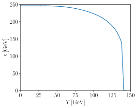
(a) Evolution of $v$.

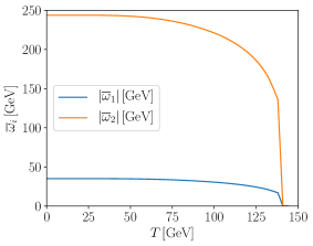
(b) Evolution of the doublet VEVs $\bar{\omega}_{k}$ ($k=1,2$).

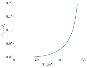
(c) Evolution of the CP-violating phase $\tan(\varphi)=\bar{\omega}_{\text{CP}}/\bar{\omega}_{2}$ of the second doublet.

(d) Evolution of the CP-violating VEV $\bar{\omega}_{\text{CP}}$ and the charge-breaking VEV $\bar{\omega}_{\text{CB}}$.

Figure 2: The temperature evolution obtained by VEVEVO for the C2HDM parameter point Eq. (5.203).

6 How to add a New Model

In this section we describe how a new model can be added to the program. To illustrate this, we have generated the template class ClassTemplate.cpp, located in the directory BSMPT/src/models/, in which the functions (according to the given comments) have to be edited. The functions to be modified are

• Class_Template

• ReadAndSet

• addLegendCT

• addLegendTemp

• addLegendTripleCouplings

• addLegendVEV

• set_gen

• set_CT_Pot_Par

• write

• TripleHiggsCouplings

• calc_CT

• MinimizeOrderVEV

• SetCurvatureArrays

• CalculateDebyeSimplified

• VTreeSimplified

• VCounterSimplified

• Debugging

Furthermore, the constant of the new model with which it is selected by the program (through Model) has to be defined in the file IncludeAllModels.h. After doing so, in the file
IncludeAllModels.cpp the corresponding entry in the function Fchoose has to be added, and the file needs to be extended to include the new model. Additionally, in ClassTemplate.h the parameters of the model have to be declared. All these files are also located in BSMPT/src/models/.

6.1 Example

As example we take a model with one scalar particle $\phi$ which develops a VEV $v$, couples to one fermion $t$ with the Yukawa coupling $y_{t}$, and to one gauge boson $A$ with the gauge coupling $g$. The relevant pieces of the Lagrangian are given by ($\Phi=\phi+v$)

$$-\mathcal{L}_{S} =\frac{m^{2}}{2}\left(\phi+v\right)^{2}+\frac{\lambda}{4!}\left(\phi+v\right)^{4}$$ (6.211)

$$-\mathcal{L}_{F} =y_{t}t_{L}t_{R}\left(\phi+v\right)$$ (6.212)

$$\mathcal{L}_{G} =g^{2}A^{2}\left(\phi+v\right)^{2}\,.$$ (6.213)

We therefore have $i,j,k,l=1,I,J=1,2,a,b=1$ for the tensors defined in Eqs. (2.5), (2.6) and (2.7). Here $I,J=1,2$ corresponds to $t_{L}$ and $t_{R}$, the left- and right-handed projections of the fermion $t$. The tensors are given by

$$L^{i} =\left.\partial_{v}\left(-\mathcal{L}_{S}\right)\right|_{\phi=0,v=0}=0$$ (6.214)

$$L^{ij} =\left.\partial_{v}^{2}\left(-\mathcal{L}_{S}\right)\right|_{\phi=0,v=0}=m^{2}$$ (6.215)

$$L^{ijk} =\left.\partial_{v}^{3}\left(-\mathcal{L}_{S}\right)\right|_{\phi=0,v=0}=0$$ (6.216)

$$L^{ijkl} =\left.\partial_{v}^{4}\left(-\mathcal{L}_{S}\right)\right|_{\phi=0,v=0}=\lambda$$ (6.217)

$$Y^{IJk} =\begin{cases}0&I=J\;(I,J=t_{L},t_{R})\\ y_{t}&I\neq J\;(I,J=t_{L},t_{R})\end{cases}$$ (6.218)

$$G^{abij} =\partial_{A}^{2}\partial_{v}^{2}\left(\mathcal{L}_{G}\right)=4g^{2}\;.$$ (6.219)

The counterterm potential, given by Eq. (2.27), reads

$$V^{\text{CT}} =\frac{\delta m^{2}}{2}\left(\phi+v\right)^{2}+\frac{\delta\lambda}{4!}\left(\phi+v\right)^{4}+\delta T\left(\phi+v\right)\;.$$ (6.220)

Application of Eqs. (2.28) and (2.29) yields

$$\delta T+v\delta m^{2}+\frac{1}{6}v^{3}\delta\lambda =-\left.\partial_{\phi}V^{CW}\right|_{\phi=0}$$ (6.221)

$$\delta m^{2}+\frac{v^{2}}{2}\delta\lambda =-\left.\partial^{2}_{\phi}V^{CW}\right|_{\phi=0}\;.$$ (6.222)

The system of equations is overconstrained. Choosing

$$\delta T=t\;,\quad\mbox{with}\quad t\in\mathbb{R}\;,$$ (6.223)

we get

$$\delta\lambda = \frac{3t}{v^{3}}+\frac{3}{v^{3}}\left(\left.\partial_{\phi}V^{\text{CW}}\right|_{\phi=0}\right)-\frac{3}{v^{2}}\left(\left.\partial^{2}_{\phi}V^{\text{CW}}\right|_{\phi=0}\right)$$ (6.224)

$$\delta m^{2} = -\frac{3}{2v}\left(\left.\partial_{\phi}V^{\text{CW}}\right|_{\phi=0}\right)+\frac{1}{2}\left(\left.\partial^{2}_{\phi}V^{\text{CW}}\right|_{\phi=0}\right)-\frac{3t}{2v}\;.$$ (6.225)

To implement this model, several files need to be changed, as described in the following.

6.1.1 IncludeAllModels.h, IncludeAllModels.cpp, ClassTemplate.h

In IncludeAllModels.h the constant with which the program selects the new model has to be set. Please make sure that the new model number is not used already by an implemented model. The program would then not know which model to select. Choosing for the template model e.g. 5, this results in adding the line
       

const int C_ModelTemplate=5;

This model selection then has to be entered in IncludeAllModels.cpp by adding to the function Fchoose the line
       

else if(choice == C_ModelTemplate)
{
return std::unique_ptr$<$Class_Potential_Origin$>$ { new Class_Template };
}

In IncludeAllModels.cpp the new model is included by adding the line
       

#include “ClassTemplate.h”

In ClassTemplate.h the variables for the potential and for the remaining Higgs coupling parameters as well as for the counterterm constants have to be added,
       

double ms, lambda, dms, dlambda, dT, yt, g;

Here ’ms’ denotes the mass parameter squared, $m^{2}$, and ’dms’, ’dlambda’ are the counterterms $\delta m^{2}$, $\delta\lambda$.

6.1.2 ClassTemplate.cpp

We will not describe here in detail every function in Class_Template.cpp that can be modified as the functions are commented in the code. Instead, we briefly describe here the most essential parts.

Class_Template()

The numbers of Higgs particles, potential parameters, counterterms and VEVs have to be specified in the constructor Class_Template() and the variable ’Model’ has to be set to the selected model. In our simple example, this is
       

Model $\displaystyle=\text{C\_ModelTemplate};$ (6.226) NNeutralHiggs $\displaystyle=1;$ (6.227) NChargedHiggs $\displaystyle=0;$ (6.228) nPar $\displaystyle=2;$ (6.229) nParCT $\displaystyle=3;$ (6.230) nVEV $\displaystyle=1;$ (6.231) NHiggs $\displaystyle=\text{NNeutralHiggs}+\text{NChargedHiggs};$ (6.232)

When you implement a new model that is not called Template but e.g. NewModel, please make sure to replace in the corresponding .h and .cpp files the name Class_Template by the name of the newly implemented class. This means that Class_Template has to be replaced by Class_NewModel wherever it appears.

ReadAndSet(const std::string& linestr, std::vector$<$double$>$& par)

In this function the input parameters of the model are read into the vector ’par’. Each line in the input file corresponds to a new parameter point. The line to be read in is given by the string ’linestr’. Via ’std::stringstream’ the parameters of each line are read into double variables. In our template model the input file would contain the parameters ’ms’ and ’lambda’ so that in the program it would look like this:
       

std::stringstream ss(linestr); double tmp; double lms,llambda; $\displaystyle\text{for(int k=1;k}<=\text{2;k++)}$ { $\displaystyle\hskip 20.00003pt\text{ss}>>\text{tmp;}$ if(k==1) lms = tmp; else if(k==2) llambda = tmp; } par[0] = lms; par[1] = llambda;

set_gen(const std::vector$<$double$>$& par)

Here, the potential parameters are set from the vector ’par’ read in with the function ReadAndSet(std::string linestr, double* par), as well as the coupling parameters. In our sample model, the gauge coupling $g$ is given by the SM gauge coupling, and the Yukawa coupling $y_{t}$ is given in terms of the SM VEV and the top quark mass. The SM gauge coupling, the SM VEV and the top quark mass are defined in $BSMPT/src/models/SMparam.h. With the parameters ’ms’ and ’lambda’ this would then look like:
       

ms $\displaystyle=\text{p}[0];$ lambda $\displaystyle=\text{p}[1];$ g $\displaystyle=\text{C\_g};$ yt $\displaystyle=\text{std::sqrt(2)/C\_vev0 * C\_MassTop};$

More complicated Higgs sectors require additional parameters. Furthermore, you can set here the potential parameters that are not read in from the input parameters but are calculated through the tree-level minimum conditions, like $m_{11}^{2},m_{22}^{2}$ and $\mbox{Im}(m_{12}^{2})$ in the C2HDM e.g. This function is also used to define the vectors vevTree and vevTreeMin. The former vector refers to the complete field configuration appearing in the effective potential. The size of the vector is hence given by $n_{\text{Higgs}}$ (cf. Sec. 2.1). For the (C)2HDM e.g., we would have $n_{\text{Higgs}}=8$ corresponding to the eight real fields $\phi_{i}$ in Eq. (3.77) (Eq. (3.118)). The vector vevTreeMin corresponds to the VEVs at $T=0$. Its size is given by the field configurations that develop a VEV, i.e. $n_{v}$ (cf. Sec. 2.3). This would be $n_{v}=4$ in the (C)2HDM, corresponding to the four VEVs $v_{1},v_{2},v_{\text{CP}}$ and $v_{\text{CB}}$. In our simple template model $n_{\text{Higgs}}$ and $n_{v}$ coincide resulting in two vectors vevTree and vevTreeMin of dimension 1 each. The value of vevTreeMin is given by the SM VEV ’C_vev0’ that is hard-coded in the program. In our sample model it would look like this:
       

$\displaystyle\text{vevTreeMin.resize(nVEV)}\,;$ $\displaystyle\text{vevTreeMin}[0]=\text{C\_vev0}\,;$ $\displaystyle\text{vevTree.resize(NHiggs)}\,;$ $\displaystyle\text{MinimizeOrderVEV(vevTreeMin,vevTree)}\,;$

Additionally, the $\overline{\mbox{MS}}$ renormalization scale can be changed here through the command
       

scale $\displaystyle=\text{mu};$

Here ’mu’ is the chosen value in GeV for the renormalization scale. The default value is ’mu = C_vev0’, i.e. the EW VEV.

MinimizeOrderVEV(const std::vector$<$double$>$& vevminimizer,
std::vector$<$double$>$& vevFunction)

Whenever we deal with the Higgs potential in the calculation, the dimension of the vector describing the fields is $n_{\text{Higgs}}$. Not all of these fields develop VEVs, however, so that the vector used in the minimizer only has dimension $n_{v}$. The function MinimizeOrderVEV is used to convert the resulting vector from the minimizer to the vector with the $n_{\text{Higgs}}$ entries. In order to do so the field(s) that develop(s) VEV(s) have to be selected. In the template model we have only one field and it develops a VEV so that we simply have to set
       

VevOrder[0] $\displaystyle=0\,;$

In a more complex model with e.g. two fields where only one of them develops a VEV, one would have to set ’$\text{VeVOrder}[0]=0$’ if the field developing the VEV is in the first entry of the vector describing the fields, and ’$\text{VeVOrder}[0]=1$’ if it is the field in the second entry.

SetCurvatureArrays()

The tensors of the Lagrangian of the new model have to be implemented in the function SetCurvatureArrays(). The notation is
       

$\displaystyle\text{Curvature\_Higgs\_L1}[i]$ $\displaystyle=L^{i}$ $\displaystyle\text{Curvature\_Higgs\_L2}[i][j]$ $\displaystyle=L^{ij}$ $\displaystyle\text{Curvature\_Higgs\_L3}[i][j][k]$ $\displaystyle=L^{ijk}$ $\displaystyle\text{Curvature\_Higgs\_L4}[i][j][k][l]$ $\displaystyle=L^{ijkl}$ $\displaystyle\text{Curvature\_Gauge\_G2H2}[a][b][i][j]$ $\displaystyle=G^{abij}$ $\displaystyle\text{Curvature\_Quark\_F2H1}[I][J][k]$ $\displaystyle=Y^{IJk}\,.$

Technically, one could use ’Curvature_Quark_F2H1’ to store all quarks and leptons there, but as they do not mix the program provides besides ’Curvature_Quark_F2H1’ where $I,J$ run over all quarks, also the structure ’Curvature_Lepton_F2H1[I][J][k]’ where $I,J$ run over all leptons. For our example this would look like
       

$\displaystyle\text{Curvature\_Higgs\_L1}[0]$ $\displaystyle=0;$ $\displaystyle\text{Curvature\_Higgs\_L2}[0][0]$ $\displaystyle=\text{ms};$ $\displaystyle\text{Curvature\_Higgs\_L3}[0][0][0]$ $\displaystyle=0;$ $\displaystyle\text{Curvature\_Higgs\_L4}[0][0][0][0]$ $\displaystyle=\text{lambda};$ $\displaystyle\text{Curvature\_Gauge\_G2H2}[0][0][0][0]$ $\displaystyle=\text{4*std::pow(g,2)};$ $\displaystyle\text{Curvature\_Quark\_F2H1}[0][0][0]$ $\displaystyle=0;$ $\displaystyle\text{Curvature\_Quark\_F2H1}[1][0][0]$ $\displaystyle=\text{yt};$ $\displaystyle\text{Curvature\_Quark\_F2H1}[0][1][0]$ $\displaystyle=\text{yt};$ $\displaystyle\text{Curvature\_Quark\_F2H1}[1][1][0]$ $\displaystyle=0;$

set_CT_Pot_Par(const std::vector$<$double$>$& par)

For the use of the counterterms, the corresponding vectors for the counterterm potential have to be set. They are named ’Curvature_Higgs_CT_L1’, ’Curvature_Higgs_CT_L2’, ’Curvature_Higgs_CT_L3’ and
’Curvature_Higgs_CT_L4’ and defined analogously to ’Curvature_Higgs_L1’ to
’Curvature_Higgs_L4’.

calc_CT( std::vector$<$double$>$& par)

The counterterms are computed numerically in the function calc_CT( std::vector$<$double$>$& par). To do so, the user has to implement the formulae for the counterterms that were derived beforehand analytically in terms of the derivatives of the Coleman-Weinberg potential, cf. Eqs. (6.223), (6.224) and (6.225) for our template model. The derivatives of $V^{\text{CW}}$ are provided by the program through the function calls WeinbergFirstDerivative and WeinbergSecondDerivative. In detail, to calculate the counterterms $\delta m^{2}$, $\delta\lambda$ and $\delta T$ of the template model, the following steps have to be performed:

• To calculate the first and second derivative of the Coleman-Weinberg potential call
         

  std::vector$\langle$double$\rangle$ WeinbergNabla,WeinbergHesse;
  WeinbergFirstDerivative(WeinbergNabla);
  WeinbergSecondDerivative(WeinbergHesse);

  
  and to save it in a vector and matrix class use
         

  VectorXd NablaWeinberg(NHiggs);
  MatrixXd HesseWeinberg(NHiggs,NHiggs);
  for(int i=0;i$<$NHiggs;i++)
  {
         NablaWeinberg[i] = WeinbergNabla[i];
         for(int j=0;j$<$NHiggs;j++)
        {
               HesseWeinberg(i,j) = WeinbergHesse.at(j*NHiggs+i);
         }
  }

• Implement the previously derived formulae for the counterterms. In our example, these are Eqs. (6.223), (6.224) and (6.225), where we set $t=0$,
         

  $\displaystyle\text{dT}=$ $\displaystyle 0;$ $\displaystyle\text{dlambda}=$ 3.0/std::pow(C_vev0,3) * NablaWeinberg[0] $\displaystyle-\text{ 3.0/std::pow(C\_vev0,2) * \text{HesseWeinberg(0,0)}};$ $\displaystyle\text{dms}=$ $\displaystyle\text{-3.0/(2*C\_vev0) * \text{NablaWeinberg[0]} + 1.0/2.0 *\text{HesseWeinberg(0,0)}};$

• Insert the parameters in the vector ’par’,
         

  $\displaystyle\text{par}[0]$ $\displaystyle=\text{dT};$ $\displaystyle\text{par}[1]$ $\displaystyle=\text{dms};$ $\displaystyle\text{par}[2]$ $\displaystyle=\text{dlambda};$

• Finally call
         

  set_CT_Pot_Par(par);

  
  so that everything is set correctly.

Afterwards, the values for dT, dmS and dlambda are set from the vector ’par’ by the function set_CT_Pot_Par(const std::vector$<$double$>$& par).

TripleHiggsCouplings()

This function provides the trilinear loop-corrected Higgs self-couplings as obtained from the effective potential. They are calculated from the third derivative of the Higgs potential with respect to the Higgs fields in the gauge basis and then rotated to the mass basis. Since the Higgs fields are ordered by mass, i.e. we have ascending indices with ascending mass, and the mass order can change with each parameter point, this implies that for each parameter point the indices of the vector containing the trilinear Higgs coupling would refer to different Higgs bosons. Therefore, it is necessary to order the Higgs bosons in the mass basis irrespective of the mass order. This order is defined through the vector HiggsOrder(NHiggs).
       

for(int i=0;i$<$NHiggs;i++)
{
       HiggsOrder[i]= value;
}

The number ’value’ is defined by the user according to the ordering that this desired in the mass basis. Thus HiggsOrder$[0]=5$ e.g. would assign the 6th lightest particle to the first position. The particles can be selected through the mixing matrix elements.

addLegendTripleCouplings()

All the following functions addLegend... extend the legends of the output files by certain variables. The function addLegendTripleCouplings extends the legend by the column names for the trilinear Higgs couplings derived from the tree-level, the counterterm and the Coleman-Weinberg potential. In order to do so, the user first has to make sure to define the names of the Higgs particles of the model in the vector ’particles’. In our model we only have one Higgs particle that we call $H$ and hence set ’particles[0]=”H”;’.

addLegendTemp()

Here the column names for $T_{c}$, $v_{c}$ and the VEVs are added to the legend. The order should be $T_{c}$, $v_{c}$ and then the names of the individual VEVs. These VEVs have to be added in the same order as given in the function MinimizeOrderVEV.

addLegendVEV()

This function adds the column names for the VEVs that are given out. The order has to be the same as given in the function MinimizeOrderVEV.

addLegendCT()

In this function, the legend for the counterterms is added. The order of the counterterms has to be same as the one set in the function set_CT_Pot_Par(par).

VTreeSimplified, VCounterSimplified

The functions
VTreeSimplified(const std::vector$<$double$>$& v) and
VCounterSimplified(const std::vector$<$double$>$& v) can be used to explicitly implement the formulae for the tree-level and counterterm potential in terms of the classical fields $\omega$, in our example these are Eqs. (6.211) and Eq. (6.220), respectively, with $\phi=0$ and $v\mathrel{\stackon[1.5pt]{=}{\stretchto{\scalerel*[\widthof{=}]{\wedge}{\rule{4.30554pt}{12.91663pt}}}{0.5ex}}}\omega$. Implementing these may improve the runtime of the programs. An example is given in the template class.

CalculateDebyeSimplified(), CalculateDebyeGaugeSimplified()

The functions
CalculateDebyeSimplified() and CalculateDebyeGaugeSimplified() can be used to implement explicit formulae for the daisy corrections to the masses of the scalars, cf. Eq. (2.32), and gauge bosons, Eq. (2.33), respectively. This is done by setting the vectors ’DebyeHiggs’ and ’DebyeGauge’ and finishing the function with a return true statement.

write()

The function write() can be used to give a terminal output of the potential parameters. For our example this would be
       

std::cout $\displaystyle<<\text{"The parameters are : " $<<$ std::endl;}$ std::cout $\displaystyle<<\text{"lambda = " $<<$ lambda $<<$ std::endl}$ $\displaystyle<<\text{"\textbackslash tm\^{}2 = " $<<$ ms $<<$ std::endl;}$ std::cout $\displaystyle<<\text{"The counterterm parameters are : " $<<$ std::endl;}$ std::cout $\displaystyle<<\text{ "dT = "$<<$ dT $<<$ std::endl}$ $\displaystyle<<\text{"dlambda = " $<<$ dlambda $<<$ std::endl}$ $\displaystyle<<\text{"dm\^{}2 = "$<<$ dms $<<$ std::endl;}$ std::cout $\displaystyle<<\text{"The scale is given by mu = " $<<$ scale $<<$ " GeV " $<<$ std::endl;}$

7 Summary

We have presented the C++ package BSMPT for the investigation of electroweak baryogenesis in extended Higgs sectors beyond the SM. The package calculates the loop-corrected effective potential at finite temperature including daisy resummations of the bosonic masses. It can be used for the computation of the VEV as a function of the temperature and in particular for the determination of $\xi_{c}=v_{c}/T_{c}$ which is related to the strength of the phase transition. Furthermore, the loop-corrected trilinear Higgs self-couplings are given out, allowing to investigate the interplay between successful baryogenesis and the required size on the Higgs self-interactions. The chosen ’on-shell’ renormalization scheme enables efficient scans in the parameter scans of the models and allows for the analysis of the connection between collider phenomenology and successful baryogenesis, so that a link between collider phenomenology and cosmology can be made. The already implemented models are the CP-conserving and CP-violating 2HDMs and the N2HDM. The program structure supports the implementation of new models, and we have illustrated with the help of a toy model how this can be done. With our new tool at hand, it is easy to further investigate the possibility of baryogenesis in new physics models, the possible spontaneous generation of CP-violating phases and make further links between collider observables and phenomena like e.g. gravitational waves. The program is constantly updated to include new phenomenologically interesting models. We are grateful for suggestions.

References

- [1] C. L. Bennett et al. [WMAP Collaboration], Astrophys. J. Suppl. 208 (2013) 20 [arXiv:1212.5225 [astro-ph.CO]].
- [2] V. A. Kuzmin, V. A. Rubakov and M. E. Shaposhnikov, Phys. Lett. B 155 (1985) 36.
- [3] A. G. Cohen, D. B. Kaplan and A. E. Nelson, Nucl. Phys. B 349 (1991) 727.
- [4] A. G. Cohen, D. B. Kaplan and A. E. Nelson, Ann. Rev. Nucl. Part. Sci. 43 (1993) 27 [hep-ph/9302210].
- [5] M. Quiros, Helv. Phys. Acta 67 (1994) 451.
- [6] V. A. Rubakov and M. E. Shaposhnikov, Usp. Fiz. Nauk 166 (1996) 493 [Phys. Usp. 39 (1996) 461] [hep-ph/9603208].
- [7] K. Funakubo, Prog. Theor. Phys. 96 (1996) 475 [hep-ph/9608358].
- [8] M. Trodden, Rev. Mod. Phys. 71 (1999) 1463 [hep-ph/9803479].
- [9] W. Bernreuther, Lect. Notes Phys. 591 (2002) 237 [hep-ph/0205279].
- [10] D. E. Morrissey and M. J. Ramsey-Musolf, New J. Phys. 14 (2012) 125003 [arXiv:1206.2942 [hep-ph]].
- [11] A.D. Sakharov, ZhETF Pis’ma 5 (1967) 32 (JETP Letters 5 (1967) 24).
- [12] K. Kajantie, K. Rummukainen and M. E. Shaposhnikov, Nucl. Phys. B 407 (1993) 356 [hep-ph/9305345]; Z. Fodor, J. Hein, K. Jansen, A. Jaster and I. Montvay, Nucl. Phys. B 439 (1995) 147 [hep-lat/9409017]; K. Kajantie, M. Laine, K. Rummukainen and M. E. Shaposhnikov, Nucl. Phys. B 466 (1996) 189 [hep-lat/9510020]; K. Jansen, Nucl. Phys. Proc. Suppl. 47 (1996) 196 [hep-lat/9509018].
- [13] K. Kajantie, M. Laine, K. Rummukainen and M. E. Shaposhnikov, Phys. Rev. Lett. 77 (1996) 2887 [hep-ph/9605288]; F. Csikor, Z. Fodor and J. Heitger, Phys. Rev. Lett. 82 (1999) 21 [hep-ph/9809291]; J. M. Cline, hep-ph/0609145.
- [14] G. D. Moore, Phys. Rev. D 59 (1999) 014503.
- [15] S. Coleman and E. Weinberg, Phys. Rev. D 7 (1973) 1888.
- [16] M. Quiros, hep-ph/9901312.
- [17] L. Dolan and R. Jackiw, Phys. Rev. D 9 (1974) 3320.
- [18] M. E. Carrington, Phys. Rev. D 45 (1992) 2933.
- [19] R. R. Parwani, Phys. Rev. D 45 (1992) 4695 Erratum: [Phys. Rev. D 48 (1993) 5965].
- [20] P. B. Arnold and O. Espinosa, Phys. Rev. D 47 (1993) 3546 Erratum: [Phys. Rev. D 50 (1994) 6662] [hep-ph/9212235].
- [21] P. Basler, M. Krause, M. Muhlleitner, J. Wittbrodt and A. Wlotzka, JHEP 1702 (2017) 121 [arXiv:1612.04086 [hep-ph]].
- [22] P. Basler, M. Mühlleitner and J. Wittbrodt, arXiv:1711.04097 [hep-ph], accepted by JHEP.
- [23] J. E. Camargo-Molina, A. P. Morais, R. Pasechnik, M. O. P. Sampaio and J. Wessén, JHEP 1608 (2016) 073 [arXiv:1606.07069 [hep-ph]].
- [24] A. Fowlie, arXiv:1802.02720 [hep-ph].
- [25] E. J. Weinberg and A. Q. Wu, Phys. Rev. D 36 (1987) 2474.
- [26] E. Benazera, N. Hansen, libcmaes, https://github.com/beniz/libcmaes.
- [27] R. Coimbra, M. O. P. Sampaio and R. Santos, Eur. Phys. J. C 73 (2013) 2428 [arXiv:1301.2599 [hep-ph]].
- [28] R. Costa et al., ScannerS project, http://scanners.hepforge.org (2016).
- [29] Jonas Müller, “Electroweak Phase Transition in N2HDM”. Available at: https://www.itp.kit.edu/_media/publications/thesis_jonas_mueller.pdf, Master Thesis, Karlsruhe Institute of Technology, 2017.
- [30] T. D. Lee, Phys. Rev. D 8 (1973) 1226.
- [31] G. C. Branco, P. M. Ferreira, L. Lavoura, M. N. Rebelo, M. Sher and J. P. Silva, Phys. Rept. 516 (2012) 1 [arXiv:1106.0034 [hep-ph]].
- [32] S. L. Glashow and S. Weinberg, Phys. Rev. D 15 (1977) 1958.
- [33] E. A. Paschos, Phys. Rev. D 15 (1977) 1966.
- [34] I. F. Ginzburg, M. Krawczyk and P. Osland, In *Seogwipo 2002, Linear colliders* 90-94 [hep-ph/0211371].
- [35] D. Fontes, J. C. Romao and J. P. Silva, JHEP 1412 (2014) 043 [arXiv:1408.2534 [hep-ph]].
- [36] W. Khater and P. Osland, Nucl. Phys. B 661 (2003) 209 [hep-ph/0302004]; A. W. El Kaffas, P. Osland and O. M. Ogreid, Nonlin. Phenom. Complex Syst. 10 (2007) 347 [hep-ph/0702097 [HEP-PH]]; B. Grzadkowski and P. Osland, Phys. Rev. D 82 (2010) 125026; A. Arhrib, E. Christova, H. Eberl and E. Ginina, JHEP 1104 (2011) 089 [arXiv:1011.6560 [hep-ph]]; A. Barroso, P. M. Ferreira, R. Santos and J. P. Silva, Phys. Rev. D 86 (2012) 015022 [arXiv:1205.4247 [hep-ph]]; S. Inoue, M. J. Ramsey-Musolf and Y. Zhang, Phys. Rev. D 89 (2014) no.11, 115023 [arXiv:1403.4257 [hep-ph]]; K. Cheung, J. S. Lee, E. Senaha and P. Y. Tseng, JHEP 1406 (2014) 149 [arXiv:1403.4775 [hep-ph]]; D. Fontes, J. C. Romao, R. Santos and J. P. Silva, JHEP 1506 (2015) 060 [arXiv:1502.01720 [hep-ph]]; C. Y. Chen, S. Dawson and Y. Zhang, JHEP 1506 (2015) 056 [arXiv:1503.01114 [hep-ph]]; R. Grober, M. Muhlleitner and M. Spira, Nucl. Phys. B 925 (2017) 1 [arXiv:1705.05314 [hep-ph]]; D. Fontes, M. Mühlleitner, J. C. Romão, R. Santos, J. P. Silva and J. Wittbrodt, JHEP 1802 (2018) 073 [arXiv:1711.09419 [hep-ph]].
- [37] M. Mühlleitner, M. O. P. Sampaio, R. Santos and J. Wittbrodt, JHEP 1708 (2017) 132 [arXiv:1703.07750 [hep-ph]].
- [38] X. G. He, T. Li, X. Q. Li, J. Tandean and H. C. Tsai, Phys. Rev. D 79 (2009) 023521 [arXiv:0811.0658 [hep-ph]]; B. Grzadkowski and P. Osland, Phys. Rev. D 82 (2010) 125026 [arXiv:0910.4068 [hep-ph]]; H. E. Logan, Phys. Rev. D 83 (2011) 035022 [arXiv:1010.4214 [hep-ph]]; M. S. Boucenna and S. Profumo, Phys. Rev. D 84 (2011) 055011 [arXiv:1106.3368 [hep-ph]]; X. G. He, B. Ren and J. Tandean, Phys. Rev. D 85 (2012) 093019 [arXiv:1112.6364 [hep-ph]]; Y. Bai, V. Barger, L. L. Everett and G. Shaughnessy, Phys. Rev. D 88 (2013) 015008 [arXiv:1212.5604 [hep-ph]]; X. G. He and J. Tandean, Phys. Rev. D 88 (2013) 013020 [arXiv:1304.6058 [hep-ph]]; Y. Cai and T. Li, Phys. Rev. D 88 (2013) no.11, 115004 [arXiv:1308.5346 [hep-ph]]; J. Guo and Z. Kang, Nucl. Phys. B 898 (2015) 415 [arXiv:1401.5609 [hep-ph]]; L. Wang and X. F. Han, Phys. Lett. B 739 (2014) 416 [arXiv:1406.3598 [hep-ph]]; A. Drozd, B. Grzadkowski, J. F. Gunion and Y. Jiang, JHEP 1411 (2014) 105 [arXiv:1408.2106 [hep-ph]]; R. Campbell, S. Godfrey, H. E. Logan, A. D. Peterson and A. Poulin, Phys. Rev. D 92 (2015) no.5, 055031 [arXiv:1505.01793 [hep-ph]]; A. Drozd, B. Grzadkowski, J. F. Gunion and Y. Jiang, JCAP 1610 (2016) no.10, 040 [arXiv:1510.07053 [hep-ph]]; S. von Buddenbrock et al., Eur. Phys. J. C 76 (2016) no.10, 580 [arXiv:1606.01674 [hep-ph]].
- [39] C. Y. Chen, M. Freid and M. Sher, Phys. Rev. D 89 (2014) no.7, 075009 [arXiv:1312.3949 [hep-ph]].
- [40] M. Muhlleitner, M. O. P. Sampaio, R. Santos and J. Wittbrodt, JHEP 1703 (2017) 094 [arXiv:1612.01309 [hep-ph]].
- [41] M. Krause, D. Lopez-Val, M. Muhlleitner and R. Santos, JHEP 1712 (2017) 077 arXiv:1708.01578 [hep-ph].
- [42] M. Galassi et al., GNU Scientific Library Reference Manual 3rd Edition, url=http://www.gnu.org/software/gsl/.
- [43] G. Guennebaud, B. Jacob et al., Eigen v3 (2010), url=http://eigen.tuxfamily.org.