A Detection of the Environmental Dependence of the Sizes and Stellar Haloes of Massive Central Galaxies

Abstract

We use ${\sim}100$ deg² of deep ($>28.5$ mag arcsec^-2 in $i$-band), high-quality (median 0.6^′′seeing) imaging data from the Hyper Suprime–Cam (HSC) survey to reveal the halo mass dependence of the surface mass density profiles and outer stellar envelopes of massive galaxies. The $i$-band images from the HSC survey reach ${\sim}4$ magnitudes deeper than Sloan Digital Sky Survey and enable us to directly trace stellar mass distributions to 100 kpc without requiring stacking. We conclusively show that, at fixed stellar mass, the stellar profiles of massive galaxies depend on the masses of their dark matter haloes. On average, massive central galaxies with $\log_{10}(M_{\star,100\mathrm{kpc}}/M_{\odot})$$>11.6$ in more massive haloes at $0.3<z<0.5$ have shallower inner stellar mass density profiles (within ${\sim}10$–$20$ kpc) and more prominent outer envelopes. These differences translate into a halo mass dependence of the mass–size relation. Central galaxies in haloes with $\log_{10}(M_{\mathrm{200b}}/M_{\odot})$$>14.0$ are $\sim 20$% larger in $R_{\mathrm{50}}$ at fixed $M_{\star,100\mathrm{kpc}}$. Such dependence is also reflected in the relationship between the stellar mass within 10 and 100 kpc. Comparing to the mass–size relation, the $M_{\star,100\mathrm{kpc}}$–$M_{\star,10\mathrm{kpc}}$ relation avoids the ambiguity in the definition of size, and can be straightforwardly compared with simulations. Our results demonstrate that, with deep images from HSC, we can quantify the connection between halo mass and the outer stellar halo, which may provide new constraints on the formation and assembly of massive central galaxies.

1 Introduction

A key discovery in the last decade has been the dramatic structural transformation of massive quiescent galaxies (e.g., Trujillo et al., 2006; van Dokkum et al., 2008; Cimatti et al., 2008; Damjanov et al., 2009; van der Wel et al., 2011; Szomoru et al., 2012; Patel et al., 2013) from $z\approx 2$ to the present day. These observations suggest that the progenitors of $z{\sim}0$ massive early-type galaxies (ETGs) need to increase their effective radii ($R_{\rm e}$) by a factor of 2–4 over a time span of 10 Gyrs (e.g., Newman et al. 2012; van der Wel et al. 2014). This observational result spurred the development of the ‘two-phase’ formation scenario for massive ETGs (e.g., Oser et al. 2010, 2012), in which galaxies form a compact central region at $z\sim 2$ through highly dissipative processes (e.g., gas-rich mergers or cold gas-accretion; Hopkins et al. 2008; Dekel et al. 2009). They subsequently assemble extended stellar haloes via dry mergers (e.g., Naab et al., 2006; Khochfar & Silk, 2006; Oser et al., 2010, 2012), which can cause significant size growth at late times. An alternative explanation for size growth, progenitor bias, hypothesizes that larger ETGs were quenched more recently; but this explanation is still under active debate (e.g., Newman et al. 2012; Carollo et al. 2013; Poggianti et al. 2013; Belli et al. 2015; Keating et al. 2015; Fagioli et al. 2016).

There have been multiple observational attempts to test the two-phase formation scenario using galaxies at low redshift, by investigating surface brightness or mass density profiles (e.g., Huang et al. 2013a, b; Oh et al. 2017), optical colour gradients (e.g., La Barbera et al. 2010; La Barbera et al. 2012), and stellar population gradients (e.g., Coccato et al., 2010, 2011; Greene et al., 2015; Barbosa et al., 2016). These observations are generally consistent with the two-phase formation scenario. However, it is still not clear whether this picture correctly predicts the connection between the stellar mass distributions in massive galaxies and their dark matter haloes.

In the $\Lambda$CDM cosmology, the assembly of massive ETGs is intrinsically tied to the hierarchical growth of their host dark matter haloes (e.g., Leauthaud et al. 2012; Behroozi et al. 2013; Shankar et al. 2013). Hydrodynamic simulations suggest that the fraction of stars accreted through mergers (the ex situ component) in central galaxies increases with halo mass (e.g., Rodriguez-Gomez et al. 2016; Pillepich et al. 2017). The major merger rate is not a strong function of progenitor halo mass (e.g., Shankar et al. 2015) but minor mergers rate should increase with halo mass, hence play an important role in determining the structures of central galaxies (e.g., Guo et al. 2011; Yoon et al. 2017). Minor mergers are efficient at ‘puffing up’ the outskirts of massive galaxies (e.g., Oogi & Habe 2013; Bédorf & Portegies Zwart 2013). Because the minor merger rate increases with halo mass, the structures of massive ETGs and the well-known stellar mass–effective radius relation ($M_{\star}$–$R_{\rm e}$; e.g., Shen et al. 2003; Guo et al. 2009) should depend on their ‘environment’ (e.g., Shankar et al. 2013; Shankar et al. 2014). However, evidence for the environment-dependence of $M_{\star}$–$R_{\rm e}$ at low redshift is still not very solid (Nair et al. 2010; Huertas-Company et al. 2013; but also see Yoon et al. 2017), and the results at higher redshift are even more unclear (e.g., Papovich et al. 2012; Lani et al. 2013; Delaye et al. 2014; but also see Rettura et al. 2010).

Deep images of massive galaxies can probe their outer stellar halos of massive galaxies and test these predictions. Unfortunately, this is observationally challenging since the stellar haloes of massive galaxies can extend to $>100$ kpc (e.g., Tal & van Dokkum 2011; D’Souza et al. 2014), and their surface brightness profiles decline rapidly with typical values of $\mu>26.0$ mag arcsec^-2 in $i$-band at 100 kpc and at $z\sim 0.3$. In Huang et al. (2017, Paper I hereafter), we showed that deep, multi-band imaging from the Subaru Strategic Program (SSP; Aihara et al. 2017a, b) using Hyper Suprime-Cam (HSC; Miyazaki et al. 2012, Miyazaki in prep.) allows us to extract robust surface stellar mass density ($\mu_{\star}$) profiles for individual galaxies with $\log_{10}(M_{\star}/M_{\odot})$$>11.4$ at $0.3<z<0.5$ and out to 100 kpc. In Paper I, we characterized the stellar mass profiles of massive ETGs and showed that there is a large intrinsic scatter in the stellar haloes of massive galaxies on 100-kpc scales. In this paper, we investigate whether the large scatter in the outer profiles of massive galaxies correlates with halo mass. We conclusively show that the sizes and stellar haloes of massive central galaxies depend on dark matter halo mass. In other words, we reveal the halo mass dependence of the mass–size relation for massive ETGs.

This paper is organized as follows. In §2 we briefly introduce the sample selection and the data reduction processes. Please refer to Huang et al. (2017) for more technical details. Our main results are presented in §3 and discussed in §4. Our summary and conclusions are presented in §5.

Magnitudes use the AB system (Oke & Gunn 1983), and are corrected for galactic extinction using calibrations from Schlafly & Finkbeiner (2011). We assume $H_{0}$ = 70 km s^-1 Mpc^-1, ${\Omega}_{\rm m}=0.3$, and ${\Omega}_{\rm\Lambda}=0.7$. Stellar mass is denoted $M_{\star}$ and has been derived using a Chabrier initial mass function (IMF; Chabrier 2003). Halo mass is defined as $M_{\rm 200b}\equiv M(<r_{\rm 200b})=200\bar{\rho}\frac{4}{3}\pi r_{\rm 200b}^{3}$, where $r_{\rm 200b}$ is the radius at which the mean interior density is equal to 200 times the mean matter density ($\bar{\rho}$). As in Huang et al. (2017), we do not attempt to decompose or distinguish any potential ‘intra-cluster’ component (ICL; e.g., Carlberg et al. 1997; Lin & Mohr 2004; Gonzalez et al. 2005; Mihos et al. 2005).

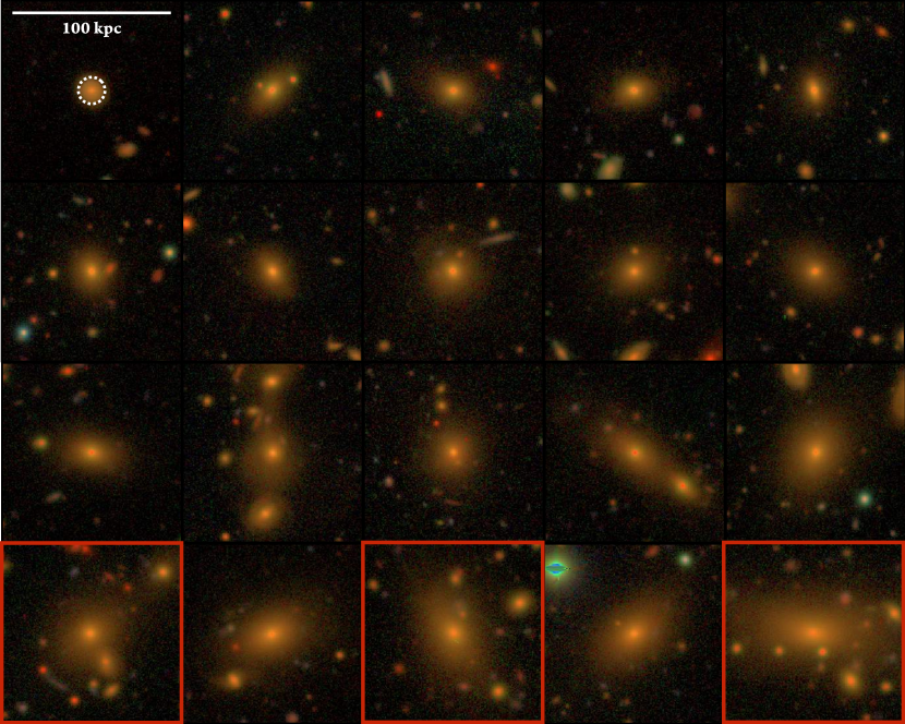
Figure 1: Three-colour images for a subsample of massive galaxies at $z{\sim}0.4$. All of these massive galaxies have very similar $M_{\star}$ within a 10-kpc elliptical aperture ($11.2<\log_{10}(M_{\star,10\ \mathrm{kpc}}/M_{\odot})<11.3$). The dashed-line circle at the top-left figure indicates $R=$10 kpc. These galaxies are rank-ordered from top to bottom and from left to right by their $M_{\star}$ within a 100-kpc elliptical aperture that varies from $10^{11.2}\ M_{\odot}$ to $10^{11.7}\ M_{\odot}$. At fixed ‘inner’ mass ($M_{\star,10\mathrm{kpc}}$), massive galaxies display significant diversity in their outer profiles. Red boxes indicate galaxies from dark matter haloes that are more massive than ${\sim}10^{14}\ M_{\odot}$.

2 Sample Selection and Data Reduction

We refer the reader to Paper I for an in-depth description of the sample selection and data reduction processes. Here, we briefly summarize the main steps.

We use imaging data from the HSC internal data release S15B, which is very similar to the Public Data Release 1 (Aihara et al. 2017b and covers ${\sim}110$ deg² in all five-band ($grizy$) to the full depth in the wide field. The data are reduced by hscPipe 4.0.2, a derivative of the Large Synoptic Survey Telescope (LSST) pipeline (e.g. Jurić et al. 2015; Axelrod et al. 2010), modified for HSC (Bosch et al. 2017). The pixel scale of the reduced image is $0.168$^′′. We use $i$-band images for extracting surface brightness profiles. HSC $i$-band images are typically 3–4 mag deeper than SDSS (Sloan Digital Sky Survey; e.g., Abazajian et al. 2009; Aihara et al. 2011; Alam et al. 2015) and have superb seeing conditions (mean $i$-band seeing has FWHM$=0.6$^′′).

In Paper I, we select a sample of 25286 bright galaxies with spectroscopic redshifts or reliable ‘red-sequence’ photometric redshifts (Rykoff et al. 2014) at $0.3<z<0.5$. Within this redshift range, we have a large enough volume ($\sim 5\times 10^{6}$ Mpc³) to sample the galaxy stellar mass function above $\log_{10}(M_{\star}/M_{\odot})$$>11.6$, and we can spatially resolve galaxies profiles to $\sim 5$ kpc ($1.0^{{\prime\prime}}$ corresponds to 4.4 and 6.1 kpc at $z=0.3$ and 0.5, respectively). Massive galaxies should experience little structural evolution and size growth between $z=0.5$ and 0.3 ($\sim$1.5 Gyr time span) based on model predictions (e.g., Shankar et al. 2015).

After carefully masking out surrounding neighbors and accounting for the subtraction of the background light, we derive $i$-band surface brightness profiles out to 100 kpc. We use the broadband spectral energy distributions (SED) fitting code iSEDFit (Moustakas et al. 2013) to measure $M_{\star}/L_{\star}$ ratios and $k$–corrections using five-band forced cModel magnitudes from hscPipe. We assume a Chabrier (2003) IMF, the Flexible Stellar Population Synthesis models (FSPS; v2.4; Conroy & Gunn 2010a, Conroy & Gunn 2010b), the Calzetti et al. (2000) extinction law, and a simple delayed-$\tau$ model for star formation histories (SFH). Using HSC data, we can measure the $\mu_{\star}$ profiles of massive galaxies to $\sim 100$ kpc, and we integrate these profiles within elliptical isophotal apertures at different physical radii. As explained in Paper I, we focus on the two following metric masses:

• Stellar mass within 10 kpc (hereafter noted $M_{\star,10\mathrm{kpc}}$), which we use as a proxy for the stellar mass of the in situ stellar component. This is motivated both by observations and simulations (e.g. van Dokkum et al. 2010, Rodriguez-Gomez et al. 2016). The value of 10 kpc that we quote here corresponds to the radius of the major axis of the isophotal ellipse.

• Stellar mass within 100 kpc (hereafter noted $M_{\star,100\mathrm{kpc}}$). We use $M_{\star,100\mathrm{kpc}}$ as a proxy for the ‘total’ stellar mass. In Paper I we show that $M_{\star,100\mathrm{kpc}}$ recovers more light compared to HSC cModel photometry with differences that can be a large as 0.2 dex in magnitude.

We use these two simple metric masses to explore the $M_{\star}$-dependence of the fraction of accreted stars and to reveal the diversity of stellar envelopes among massive galaxies. In practice, we also have the full profiles for each galaxy and can cast our results in terms of the full stellar mass profiles. However, in many cases we find it useful to display figures using the simpler $M_{\star,10\mathrm{kpc}}$ and $M_{\star,100\mathrm{kpc}}$ quantities. In Figure 1, we highlight the diversity of galaxies as a function of $M_{\star,10\mathrm{kpc}}$ and $M_{\star,100\mathrm{kpc}}$. Figure 1 shows a subsample of massive galaxies with very similar $M_{\star,10\mathrm{kpc}}$ but show a large range of $M_{\star,100\mathrm{kpc}}$. We use these two aperture masses to guide our comparison of massive galaxies as a function of environment.

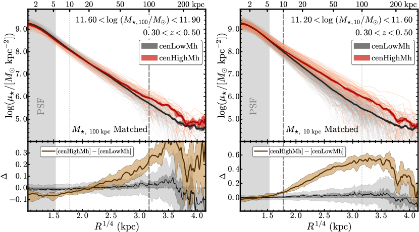
Figure 2: The environmental dependence of the stellar mass profiles of massive central galaxies. Left: Halo mass dependence of galaxy $\mu_{\star}$ profiles at fixed ‘total’ stellar mass ($M_{\star,100\mathrm{kpc}}$). Right: Halo mass dependence of galaxy $\mu_{\star}$ profiles at fixed ‘inner-mass’ ($M_{\star,10\mathrm{kpc}}$). In each plot, we match the two samples so that they share similar distributions of mass and redshift (Appendix C). We use $R^{1/4}$ as $x$–axis to provide a balanced view of both the central and outer regions of the galaxy. Orange and red lines correspond to central galaxies living in haloes with $\log_{10}(M_{\mathrm{200b}}/M_{\odot})$ $\geq 14.2$. Black and grey lines correspond to central galaxies living in haloes with $\log_{10}(M_{\mathrm{200b}}/M_{\odot})$ $\leq 14.0$. Thin lines show the profiles of individual galaxies, while thick lines show the median profile. The uncertainty on the median profile is given by the shaded region and is computed via bootstrap resampling. Brown lines in the bottom panels show the relative difference between the two median profiles ($\Delta=\log(\mu_{\star,\mathrm{cenHighMh}})-\log(\mu_{\star,\mathrm{cenLowMh}}$). Errors in the difference between the two profiles are also computed via bootstrap. The grey-shaded regions show a Monte Carlo test to assess how likely it is to obtain $\Delta$ from random sub-samples of the data. To compute the grey-shaded regions, we first mix the two samples (cenHighMh and cenLowMh), then draw sub-samples of galaxies from the mixed population and compute $\Delta$ in the same fashion as for our fiducial signal. We repeat this process 5000 times. The dark grey–shaded region (light grey–shaded region) shows the 1-$\sigma$ (3-$\sigma$) fluctuations in $\Delta$ from these 5000 draws.

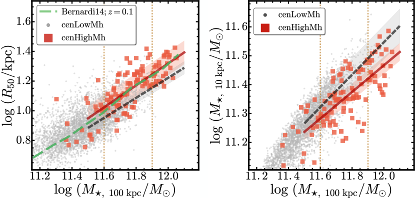
Figure 3: Left: The mass-size relations for cenHighMh (orange squares) and cenLowMh (grey dots) galaxies. Two vertical lines highlight our $11.6<$ $\log_{10}(M_{\star}/M_{\odot})$ $<11.9$ mass bin. The red solid line shows the best-fitting mass–size relation for cenHighMh and the grey dashed line shows the best-fitting relation for cenLowMh. Shaded regions in lighter colours show the 1-$\sigma$ uncertainties from Markov chain Monte Carlo (MCMC) sampling. The green dashed line shows the mass–size relation for $z\sim 0.1$ early–type galaxies from Bernardi et al. (2014). Right: The relations between $M_{\star,100\mathrm{kpc}}$ and $M_{\star,10\mathrm{kpc}}$ for the cenHighMh and cenLowMh galaxies, along with the best-fitting scaling relations for both samples.

2.1 Massive Central Galaxies from Different Environments

In this work, we focus on massive galaxies with $M_{\star,100\mathrm{kpc}}$ $>10^{11.6}$ $M_{\odot}$. In Paper I, we demonstrate that this sample is almost mass complete over our full redshift range. In addition to the mass cut above, we also limit our sample to galaxies that live at the centers of their own dark matter haloes – so-called ‘central’ galaxies. We use the redMaPPer v5.10 (Rykoff et al., 2014; Rozo et al., 2015) cluster catalogue to help us construct two central galaxy samples: one for high mass haloes, and one for low mass haloes.

First, we build a sample of central galaxies in high mass haloes. We select 68 massive central galaxies from redMaPPer clusters with richness $\lambda\geq 30$, with central probability $P_{\mathrm{Cen}}\geq 0.7$, and $\log_{10}(M_{\star,100\mathrm{kpc}}/M_{\odot})$$>11.5$ at $0.3<z<0.5$ (63/68 have $\log_{10}(M_{\star,100\mathrm{kpc}}/M_{\odot})$$>11.6$). This $\lambda$ limit is chosen to mitigate incompleteness in the cluster catalogue at the high end of our redshift window. The $P_{\mathrm{Cen}}$ limit is imposed to limit our sample to central galaxies. Simet et al. (2017) present a calibration of the $M_{\mathrm{200b}}$-$\lambda$ relation for redMaPPer clusters using SDSS weak-lensing. Based on this calibration, our sample corresponds to central galaxies living in haloes with $M_{\mathrm{200b}}$$>10^{14.2}$ $M_{\odot}$. This calibration is consistent with several other independent calibrations using different methods (e.g., Saro et al. 2015; Farahi et al. 2016; Melchior et al. 2016; Murata et al. 2017). The median richness of the sample is $\lambda\approx 41$ ($\log_{10}(M_{\mathrm{200b}}/M_{\odot})$$\approx 10^{14.3}$), and there are 44 central galaxies in clusters with $\lambda>50$ ($M_{\mathrm{200b}}$$\approx 10^{14.5}$). We refer to this sample of central galaxies in massive haloes as the cenHighMh sample.

Second, we build a sample of central galaxies in low mass haloes. We begin by excluding all galaxies in redMaPPer clusters with $\lambda>20$. We convert $\lambda$ to $M_{\mathrm{200b}}$ using the Simet et al. (2017) calibration. For each cluster, we compute $R_{\mathrm{200b}}$ using the Colossus Python package (Diemer 2015) provided by Diemer & Kravtsov (2015) We exclude all galaxies within a cylinder around each cluster, with a radius equal to $R_{\mathrm{200b}}$, and a length equal to twice the value of the photometric redshift uncertainty of the cluster (typically around 0.015 to 0.025). This second sample is dominated by central galaxies living in haloes with $M_{\mathrm{200b}}<10^{14}$ $M_{\odot}$; we refer to this sample as cenLowMh.  There are 833 central galaxies with $\log_{10}(M_{\star,100\mathrm{kpc}}/M_{\odot})$$>11.6$ in this sample.

Given the high stellar mass, satellite contamination in our sample should be low (e.g., Reid et al. 2014; Hoshino et al. 2015; Saito et al. 2016; van Uitert et al. 2016). For instance, the model from Saito et al. (2016) predicts that our cenHighMh sample should only contain $\sim 7$% satellites (corresponding to satellites with $\log_{10}(M_{\star,100\mathrm{kpc}}/M_{\odot})$$>11.6$ and living in haloes with $\log_{10}(M_{\mathrm{200b}}/M_{\odot})$$<14.0$).

Appendix A shows the distributions of redshift, $M_{\star,100\mathrm{kpc}}$, and $M_{\star,10\mathrm{kpc}}$ for the two samples. We also compare these two samples on a $M_{\star,100\mathrm{kpc}}$ versus rest–frame $(g-r)$ colour plane. Both samples follow the same red-sequence, with only a handful of galaxies displaying bluer colours. Given the available calibration, the current $\lambda$ cut should ensure the cenHighMh and cenLowMh samples have significant difference in average halo mass, although we can not directly estimate the average $\log_{10}(M_{\mathrm{200b}}/M_{\odot})$ for the cenLowMh sample. In Appendix D, we show that the main results are robust even when $\lambda>20$ cut is adopted for the cenHighMh sample.

Our analysis fails to extract 1-D profiles for $\sim 10$% of cenHighMh and cenLowMh galaxies due to ongoing major mergers or projection effects (e.g. nearby foreground galaxy or bright stars). We exclude these galaxies from our analysis and this low failure rate should not affect any of our results.

3 Results

As shown in Figure 1, massive central galaxies at fixed $M_{\star,10\mathrm{kpc}}$ display a large diversity in their stellar haloes. In Paper I, we explored the $M_{\star}$-dependence of these stellar haloes. We now investigate the relation between $\mu_{\star}$ profiles, stellar haloes, and dark matter halo mass. We remind the reader that although a circular aperture is shown on Fig 1, in practice we extract 1-D $\mu_{\star}$ profiles and estimate $M_{\star,100\mathrm{kpc}}$ and $M_{\star,10\mathrm{kpc}}$ using elliptical apertures following the average flux-weighted isophotal shape.

3.1 Environmental Dependence of the Stellar Mass Density Profiles of Massive Galaxies

First, we ask whether the $\mu_{\star}$ profiles of massive central galaxies depend on halo mass at fixed stellar mass. We show comparisons of $\mu_{\star}$ profiles at both fixed $M_{\star,100\mathrm{kpc}}$ and fixed $M_{\star,10\mathrm{kpc}}$ (see Figure 2). All comparisons are performed with a fixed underlying redshift distribution by matching samples in redshift in addition to stellar mass (see Appendix C, Appendix B, and Fig 7 for details).

Fig 2 compares the $\mu_{\star}$ profiles of massive central galaxies in low mass haloes to those in high mass haloes at fixed $M_{\star,100\mathrm{kpc}}$ (left panel) and at fixed $M_{\star,10\mathrm{kpc}}$ (right panel). The left panel compares galaxies that have similar ‘total’ stellar mass. The right panel uses $M_{\star,10\mathrm{kpc}}$ as a proxy for the in situ component to compare the profiles of galaxies that presumably have similar early formation histories, but which live in different dark matter haloes today. This figure shows the main result of this paper, namely that the $\mu_{\star}$ profiles of massive central galaxies show a clear dependence on dark matter halo mass at both fixed $M_{\star,100\mathrm{kpc}}$ and $M_{\star,10\mathrm{kpc}}$.

We estimate the uncertainties of the median $\mu_{\star}$ profiles using a bootstrap resampling test, and we perform statistical tests to demonstrate that the difference between the profiles is more significant than the level allowed by the intrinsic randomness within the combined cenHighMh and cenLowMh sample. We also conduct a variety of tests that verify the robustness of these results with respect to our $M_{\star,100\mathrm{kpc}}$ binning scheme, $\lambda$ cut, the redshift range, and the choice of apertures used for the metric masses. Please see Appendix D for further details. Appendix E and Figure 12 compares the same $M_{\star,100\mathrm{kpc}}$-matched samples using cumulative $M_{\star}$ profiles (‘curve of growth’) and the fraction of $M_{\star,100\mathrm{kpc}}$ enclosed within different radii. Both comparisons highlight the differences in the median $\mu_{\star}$ profiles from different angles.

The key features in Figure 2 are the following:

• At fixed $M_{\star,100\mathrm{kpc}}$, central galaxies in high mass haloes display shallower $\mu_{\star}$ profiles compared to those in low mass haloes (i.e., they have flatter inner $\mu_{\star}$ profiles and more significant outer stellar envelopes).

• The median $\mu_{\star}$ profiles of the two samples cross each other at ${\sim}15$-20 kpc, roughly the typical effective radius ($R_{\mathrm{e}}$) of galaxies at these masses ($\log_{10}(M_{\star,100\mathrm{kpc}}/M_{\odot})$$>11.7$–11.8).

• When matched by $M_{\star,100\mathrm{kpc}}$, differences in the inner regions appear to be small, but this is also driven by the use of a logarithmic y-axis. The difference becomes more apparent at $R>50$ kpc.

• Massive galaxies matched by $M_{\star,10\mathrm{kpc}}$ display a range of $M_{\star,100\mathrm{kpc}}$ values. Those in massive dark matter halos have more prominent outer stellar haloes. The scatter in the outer profiles observed in Figure 2 is an intrinsic scatter (not measurement error).

Fig 2 shows that the environmental dependence of the profiles of massive central galaxies is a subtle effect that is most prominent at large radii ($R>50$ kpc). This may explain why previous attempts to detect this effect using shallower images have often failed.

The effect becomes more pronounced for even more massive galaxies. This is shown in Fig 8 in Appendix D.

In summary, we detect a subtle, but robust halo mass dependence of the profiles of massive central galaxies. This dependence could be driven by the fact that massive halos have a larger minor merger rate compared to less massive haloes. Non–dissipative (minor) mergers should not strongly alter inner profiles, but can efficiently build up outer haloes (e.g., Hilz et al. 2013, Oogi & Habe 2013).

3.2 The Environmental Dependence of Scaling Relations

We have shown that the $\mu_{\star}$ profiles of massive galaxies vary with the masses of their host dark matter haloes. We now turn our attention to the more commonly studied stellar mass–size relation ($M_{\star}$–$R_{\mathrm{e}}$). In addition, we consider halo mass dependence on the $M_{\star,100\mathrm{kpc}}$–$M_{\star,10\mathrm{kpc}}$ plane.

3.2.1 Mass–Size Relation

The tight relation between $M_{\star}$ and effective radius (or half-light radius; $R_{\mathrm{e}}$ or $R_{\mathrm{50}}$; e.g., Shankar et al. 2013; Leja et al. 2013; van der Wel et al. 2014) is one of the most important scaling relationships for ETGs. Despite numerous attempts, previous studies have failed to detect the $M_{\mathrm{200b}}$-dependence of the $M_{\star}$–$R_{\mathrm{e}}$ relation at low-$z$ (e.g., Weinmann et al. 2009; Nair et al. 2010; Huertas-Company et al. 2013; Cebrián & Trujillo 2014; except for the recent result by Yoon et al. 2017).

However, ‘size’ is not a well-defined parameter for massive galaxies with very extended stellar mass distributions. In practice, measurements of the ‘effective radius’, or ‘half-light radius’, depend on resolution, depth, filter, and may also depend on the adopted model for the light profile. This makes comparisons of size measurements among different observations, or between observations and models, uncertain. This is the main reason why we prefer to compare $\mu_{\star}$ profiles directly which completely bypasses the need to consider ‘size’.

Nonetheless, to enable comparisons with past work, we now consider the more traditional mass-size relation. We adopt the radius enclosing 50% of stellar mass within 100 kpc ($R_{\mathrm{50}}$; derived from the $i$-band curve-of-growth) as our ‘size’ for massive galaxies. This definition of ‘half-light radius’ is more robust against structural details, model choice, and background subtraction, compared to the effective radius measured using oversimplified 2-D models such as the single-Sérsic  model. Massive galaxies in this sample are large enough so that the impact of seeing is not a concern.

The left panel of Fig 3 shows the mass-size relation for our two samples. We fit the $\log_{10}(M_{\star,100\mathrm{kpc}}/M_{\odot})$-$\log_{10}(R_{\mathrm{50}}/\mathrm{kpc})$ relations at $\log(M_{\star,100})>11.6$ using the emcee MCMC sampler (Foreman-Mackey et al. 2013). Uncertainties in both $M_{\star,100\mathrm{kpc}}$ and $R_{\mathrm{50}}$ are considered. For $\log_{10}(M_{\star,100\mathrm{kpc}}/M_{\odot})$$>11.6$ galaxies, the typical uncertainty for mass is $\sim 0.12$ dex. The $R_{\mathrm{50}}$ uncertainty is based on the $\mu_{\star}$ profile and is very small due to the high $\mathrm{S}/\mathrm{N}$ of the profile. We manually assign a 10% error for $R_{\mathrm{50}}$.

The best-fitting relation for cenHighMh is:

$$\log_{10}(R_{\mathrm{50}}/\mathrm{kpc})= (0.74\pm 0.13)\times\log_{10}(M_{\star,100\ \mathrm{kpc}}/M_{\odot})$$ (1)

$$-(7.56\pm 1.56)$$

And for cenLowMh, we find:

$$\log_{10}(R_{\mathrm{50}}/\mathrm{kpc})= (0.68\pm 0.06)\times\log_{10}(M_{\star,100\ \mathrm{kpc}}/M_{\odot})$$ (2)

$$-(6.88\pm 0.75)$$

As shown in the left panel of Fig 3, the two samples lie on $M_{\star,100\mathrm{kpc}}$–$R_{\mathrm{50}}$ relations that have similar slopes but different normalizations. The best-fitting mass–size relation derived here suggests that, at $0.3<z<0.5$, central galaxies with $\log_{10}(M_{\star,100\mathrm{kpc}}/M_{\odot})$$>11.6$ in $\log_{10}(M_{\mathrm{200b}}/M_{\odot})$$>14.2$ haloes are on average $\sim 20$% larger than centrals in $\log_{10}(M_{\mathrm{200b}}/M_{\odot})$$<14.0$ haloes at fixed $M_{\star,100\mathrm{kpc}}$. This result is robust against the stellar mass range over which the fit is performed and against the definitions of ‘total’ $M_{\star}$ and half-light radius.

Due to the steep slope of the mass–size relation, secondary binning (e.g., different halo mass) may introduce artificial differences (e.g., Sonnenfeld & Leauthaud 2017). Besides the differences in best–fit $M_{\star,100\mathrm{kpc}}$–$R_{\mathrm{50}}$ relation, the median $R_{\mathrm{50}}$ of the $M_{\star,100\mathrm{kpc}}$-matched samples also confirm the above conclusion. In addition, we use the normalized size parameter ($\gamma$; e.g., Newman et al. 2012; Huertas-Company et al. 2013) to further test our results. In Huertas-Company et al. (2013), $\gamma$ is defined as:

$$\log_{10}(\gamma)=\log_{10}(R_{\mathrm{50}})+\beta(11-\log_{10}M_{\star,100\ \mathrm{kpc}}),$$ (3)

where $\beta$ is the slope of the mass–size relation. We estimate the average $\gamma$ of both samples at $\log_{10}(M_{\star,100\mathrm{kpc}}/M_{\odot})$$>11.6$. For cenHighMh, $<\gamma>=4.2\pm 0.4$ and for cenLowMh, $<\gamma>=3.8\pm 0.3$. The environmental dependence of $R_{\mathrm{50}}$ at fixed $M_{\star,100\mathrm{kpc}}$ is more significant than the Huertas-Company et al. (2013) result but weaker than some model predictions (e.g., Shankar et al. 2014).

We also compare with the mass–size relation from the Figure 12 of Bernardi et al. 2014 (green dashed line). These authors studied the mass–size relation for a large sample of $z\leq 0.1$ ETGs by fitting their SDSS images with a 2–component model that consists of a Sérsic  and an exponential component (SerExp). Comparing to the single-Sérsic  model, the SerExp model provides much less biased measurements of total luminosity and effective radius for massive galaxies. The stellar masses are derived based on a $M_{\star}/L_{\star}$–color relation for SDSS $r$-band assuming a Chabrier IMF (see Bernardi et al. 2010). The mass-size relation from Bernardi et al. 2014 is qualitatively consistent with the one from this work. Differences of redshift and assumptions in stellar mass measurements between Bernardi et al. 2014 and this work can lead to systematic shifts on the mass–size plane. However, it is still interesting that the mass-size relation derived by 2–component model fitting on much shallower SDSS images has very similar slope comparing to the HSC result. The impacts of imaging depth and modeling method on the study of mass–size relation deserves further investigation using a common sample of massive galaxies in the near future.

3.2.2 $M_{\star,100\mathrm{kpc}}$ - $M_{\star,10\mathrm{kpc}}$ Relation

We now explore the environment dependence of galaxy structure using the $M_{\star,100\mathrm{kpc}}$-$M_{\star,10\mathrm{kpc}}$ relation. Compared to the mass–size relation, the $M_{\star,100\mathrm{kpc}}$–$M_{\star,10\mathrm{kpc}}$ relation is not plagued by the ambiguity of galaxy ‘size’, and it also enables a more straightforward comparison with numerical simulations.

The right panel of Fig 3 compares our two samples on the $M_{\star,100\mathrm{kpc}}$–$M_{\star,10\mathrm{kpc}}$ plane. The two samples follow distinct best-fitting $M_{\star,100\mathrm{kpc}}$–$M_{\star,10\mathrm{kpc}}$ relations. For cenHighMh galaxies with $\log_{10}(M_{\star,100\mathrm{kpc}}/M_{\odot})$$>11.6$ we find:

$$\log_{10}(M_{\star,10\ \mathrm{kpc}}/M_{\odot})= (0.48\pm 0.06)\times\log_{10}(M_{\star,100\ \mathrm{kpc}}/M_{\odot})$$ (4)

$$+(5.72\pm 0.75).$$

In the same range of $M_{\star,100\mathrm{kpc}}$, the best-fitting relation for cenLowMh is:

$$\log_{10}(M_{\star,10\ \mathrm{kpc}}/M_{\odot})= (0.56\pm 0.03)\times\log_{10}(M_{\star,100\ \mathrm{kpc}}/M_{\odot})$$ (5)

$$+(4.82\pm 0.30).$$

These results are robust against the exact choice of the stellar mass range over which the fit is performed. These results are also unchanged when we replace $M_{\star,10\mathrm{kpc}}$ with the stellar mass within a 5- or 15-kpc aperture, or if $M_{\star,100\mathrm{kpc}}$ is replaced with a stellar mass within a 120- or 150-kpc aperture.

Figure 3 presents the same conclusions as in the previous section, namely that at fixed $M_{\star,100\mathrm{kpc}}$, central galaxies of more massive haloes tend to have a smaller fraction of stellar mass in their inner regions and more prominent outer stellar haloes. And at fixed $M_{\star,10\mathrm{kpc}}$, central galaxies of more massive haloes on average are $\sim 0.1$ dex more massive than the ones from less massive haloes within a 100 kpc aperture, which corresponds to $\sim 10^{11}M_{\odot}$ of stellar mass differences. If we can assume that the same $M_{\star,10\mathrm{kpc}}$ suggests similar $M_{\star}$ when they were just quenched at high redshift (or similar in situ stellar mass), this means the central galaxies of $\log_{10}(M_{\mathrm{200b}}/M_{\odot})$$>14.2$ haloes typically experienced one more major merger or a few more minor mergers comparing to the ones of $\log_{10}(M_{\mathrm{200b}}/M_{\odot})$$<14.0$ haloes. It would be interesting to compare this prediction with hydro-simulations or semi-analytic models.

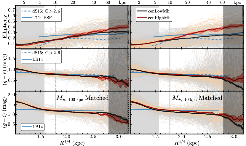
Figure 4: Radial variations in ellipticity and optical colours for massive galaxies. The format of this figure is similar to the right hand side of Fig 2. Top panels show the ellipticity profile, middle panels show $g-r$, and lower panels show $g-i$. We compare our results with those from Tal & van Dokkum (2011) (solid blue line on top panels). We also compare our results with those from a stacking analysis of nearby massive galaxies with high concentration indices ($C>2.6$) from D’Souza et al. (2014) (blue dashed lines in top and middle panels). We also compare our results with the average $g-r$ and $g-i$ colour profiles from a large sample of nearby elliptical galaxies for La Barbera et al. (2010) (blue, solid lines in middle and bottom panels).

3.3 Ellipticity and Colour Profiles

In Paper I, we show that the ellipticity of the outer stellar halo increases with stellar mass but that rest-frame colour gradients do not depend strongly on stellar mass. In this paper, we take this analysis one step further to investigate whether either of these quantities depends on halo mass. We focus on ellipticity and colour profiles within 5–60 kpc where we can ignore differences in sky subtraction and seeing across different filters. Galactic extinction and $k$ corrections are applied to both $(g-r)$ and $(g-i)$ colour profiles.

Figure 4 shows the average ellipticity, $g-r$, and $g-i$ colour profiles for galaxies at fixed $M_{\star,100\mathrm{kpc}}$ and fixed $M_{\star,10\mathrm{kpc}}$. Our main findings are:

• The ellipticity profiles of massive central galaxies do not depend on halo mass at fixed $M_{\star,100\mathrm{kpc}}$ at $R<60$ kpc (upper left panel).

• However, we do find that at fixed $M_{\star,10\mathrm{kpc}}$, galaxies in massive halos have more elliptical outer stellar halos compared to galaxies in low mass halos (upper right panel). This may be further evidence that elongated outer stellar haloes are built from accreted stars.

• We find no evidence that the rest-frame colour gradients (at $r<60$ kpc) of massive galaxies depend on halo mass.

The fact that we find smooth ellipticity profiles and shallow gradients favors the idea of using a flux-weighted average isophotal shape to extract 1-D $\mu_{\star}$ profiles for massive galaxies. The similarity in the average rest-frame colour profiles demonstrates that our results can not simply be explained by differences in radial $M_{\star}/L_{\star}$ ratios between the two samples.

Our work does not address color gradients below 5–6 kpc because we do not deconvolve for the PSF. Color gradients on these scales may be sensitive to other physical processes and deserve future investigation using 2-D modelling methods and/or images with higher spatial resolution.

4 Discussion

4.1 The Role of Environment in the Two-Phase Formation Scenario

Using deep images from the HSC survey, we show that the stellar mass distributions of massive central galaxies at $0.3<z<0.5$ depend on halo mass. At fixed total galaxy mass, central galaxies in massive halos have larger half-light radii and host more prominent outer stellar haloes compared to galaxies in low mass haloes (Figure 3). We also find that the outer stellar haloes ($R>50$ kpc) of massive galaxies show the strongest variations with halo mass.

The two-phase formation scenario can qualitatively explain these results. In this scenario, intense dissipative processes at $z>2$ are responsible for the formation of in situ stars in massive central galaxies. After a rapid quenching of star formation, the subsequent assembly of massive galaxies is dominated by the accretion of satellite galaxies through (mostly) non–dissipative mergers. Dry minor mergers are efficient at depositing ex situ stars in the outskirts of massive galaxies (e.g., Oogi & Habe 2013; Bédorf & Portegies Zwart 2013) and hence in building up outer stellar haloes. The fact that minor mergers become more frequent in more massive dark matter haloes could lead to the halo mass dependence of galaxy profiles that we identify in Figure 2.

Shankar et al. (2014) studied the environment dependence of galaxy size using semi-analytic models. They predict that at fixed stellar mass, the median size of central galaxies should increase strongly with halo mass. Although the major-merger rate does not strongly depend on halo mass (mass ratio $>1$:3; e.g., Hirschmann et al. 2013; Shankar et al. 2015), the minor–merger rate could still increase with halo mass if the dynamical friction timescale is short (e.g., Newman et al. 2012). Massive central galaxies with $11.5<$$\log_{10}(M_{\star}/M_{\odot})$$<12.0$ living in haloes with $\log_{10}(M_{\mathrm{200b}}/M_{\odot})$$>14.0$ can have up to four times more minor mergers (1:100–1:3) compared to those in less massive haloes at fixed galaxy mass. An increase in the minor-merger rate as a function of halo mass can lead to a halo-mass dependence in the mass–size relation. The predictions from Shankar et al. (2014) have been confirmed by Yoon et al. (2017) using the semi-analytic model from Guo et al. (2011).

Our results are broadly consistent with these predictions. As an important next step, we are using the HSC galaxy-galaxy weak lensing results (Mandelbaum et al. 2018) to help us achieve a more detailed picture of the environment dependence. The preliminary result so far has confirmed the trends found in this work with more straightforward and accurate constraints of halo mass (Huang  et al. in prep.). However, our results alone cannot rule out other explanations for this halo mass dependence. For instance, Buchan & Shankar (2016) suggests that, under the extreme situation that the majority of the baryons in the halo of the main progenitor can be converted into stars, the in-situ component alone can account for the environment difference we see today. Although very unlikely, it requires comparisons with high redshift observations to distinguish between these two scenarios.

4.2 The Inner Regions of Massive Galaxies

Figure 3 shows that, at fixed total galaxy mass, centrals in high mass haloes have slightly shallower inner $\mu_{\star}$ slopes and lower values of $M_{\star,10\mathrm{kpc}}$ compared to those in low mass haloes. We have tested that this cannot be solely explained by the choice of a finite aperture (100 kpc) to estimate ‘total’ galaxy mass. Integrating our profiles out to larger radii makes the differences between cenHighMh and cenLowMh galaxies on the $M_{\star,100\mathrm{kpc}}$–$M_{\star,10\mathrm{kpc}}$ plane even more significant (see Appendix D). In hydrodynamic simulations, intense dissipative processes help create a self-similar de Vaucouleurs–like ($n{\sim}4$) inner density profile (e.g., Hopkins et al. 2008). However, there are a variety of physical processes that can shape and alter the inner profile which we now discuss.

First, major mergers can redistribute the inner stellar mass distributions, but the major–merger rate does not strongly depend on halo mass (e.g., Shankar et al. 2014). However, minor mergers, which do depend on halo mass, can also modify central surface brightness profiles (e.g., Boylan-Kolchin & Ma 2007). Depending on the structure, and the orbits of infalling satellites, a minor merger can make the inner $\mu_{\star}$ profiles either steeper or shallower. Interestingly, Boylan-Kolchin & Ma (2007) find that when a satellite is accreted from a highly eccentric and energetic orbit to a core–elliptical galaxy, the process tends to reduce the central $\mu_{\star}$. This is relevant here, as many massive ETGs are known to be core–elliptical galaxies.

Second, strong adiabatic expansion induced by powerful AGN feedback is another mechanism (e.g., Fan et al. 2008; Martizzi et al. 2013) that can modify stellar density profiles. When the induced mass loss is efficient enough, it can lead to expanded central stellar mass distribution and can significantly lower the inner $\mu_{\star}$.

Finally, the coalescence of super-massive black holes (SMBHs) can also flatten the central $\mu_{\star}$ profile via an efficient scattering effect (e.g., Milosavljević et al. 2002). On the right side of Fig 3, there are a few candidates for galaxies with large cores. These may be similar to the recently discovered massive brightest cluster galaxies (BCGs) with very large depleted cores (a few thousand parsecs; e.g., Postman et al. 2012; López-Cruz et al. 2014; Thomas et al. 2016; Bonfini & Graham 2016) possibly resulting from SMBH mergers.

The impact of these processes on $\mu_{\star}$ profiles and their dependency on halo mass are important questions that warrant further investigation.

4.3 Comparison with Previous Work

Many previous studies that focused on the mass–size relation found this relation to be independent of halo mass or environment at $z\sim 0.0$ (e.g., Nair et al. 2010; Maltby et al. 2010; Cappellari 2013; Huertas-Company et al. 2013). Shallow imaging and the use of models which do not necessarily well describe massive galaxies (e.g., single-Sérsic  or de Vaucouleurs models) may have masked the effect revealed in this paper. In Appendix F, we use the cenHighMh and cenLowMh galaxies that overlap with the Galaxy And Mass Assembly (GAMA) survey to demonstrate this point. We show that, for galaxies with similar $M_{\star}$ derived from single-Sérsic  models using shallower SDSS images (Kelvin et al. 2012), the ones in more massive dark matter haloes actually show more prominent outer stellar haloes. These types of issues complicate the comparisons of mass–size relations derived from different images or using different methods. For this reason, we only present a qualitative comparison with previous work.

At low redshift, Cebrián & Trujillo (2014) find ETGs with $\log_{10}(M_{\star}/M_{\odot})$$>11.5$ to be slightly larger in more massive haloes, and they also show that this trend is reversed at lower $M_{\star}$. Kuchner et al. (2017) use one massive cluster at $z=0.44$ to show that ETGs in that cluster have larger sizes than ETGs in the ‘field’. Yoon et al. (2017) present a study of a large sample of $z\sim 0.1$ SDSS ETGs using a nonparametric method. They also find an environmental dependence of the mass–size relation at $\log_{10}(M_{\star}/M_{\odot})$$>11.2$. Similar to our work, they find that massive ETGs in dense environments are 20–40% larger compared to those in underdense environments. Recently, Charlton et al. (2017) use a single-Sérsic  model for galaxies at $0.2<z<0.8$ in the Canada France Hawaii Lensing Survey (CFHTLenS) (Heymans et al. 2012) together with galaxy–galaxy lensing measurements to show that larger galaxies tend to live in more massive dark matter haloes (also see Sonnenfeld & Leauthaud 2017). These results are in broad agreement with those presented here.

As the halo mass dependence of the sizes and $\mu_{\star}$ profiles of massive galaxies is being confirmed at low–redshift, the physical origin and redshift evolution of such dependence will become of increasing interest. Right now, some observations find a strong environmental dependence of the mass–size relation for massive quiescent or early-type galaxies at high–redshift (e.g., Papovich et al. 2012; Bassett et al. 2013; Lani et al. 2013; Strazzullo et al. 2013; Delaye et al. 2014), while other works suggest otherwise (e.g., Rettura et al. 2010; Raichoor et al. 2012; Kelkar et al. 2015; Allen et al. 2015). Comparison with high–redshift results are complicated by many issues and is beyond the scope of this work, but we want to point out again that previous works mostly focus on the mass–size relation while direct comparison of $\mu_{\star}$ profile (e.g., Szomoru et al. 2012; Patel et al. 2013; Buitrago et al. 2017; Hill et al. 2017) could help us trace the redshift evolution of the environment dependence better.

4.4 Towards Consistent Size Definitions

Until recently, semi-analytic models and hydrodynamic simulations have had difficulty reproducing the mass–size relation of massive galaxies. Galaxy sizes are sensitive to many different physical processes (star-formation, feedback, mergers), and matching the galaxy stellar-mass function does not automatically guarantee a match to the mass–size relation. Furthermore, while some effort have been made to use consistent size definitions (McCarthy et al. 2017), more often than not, comparisons of the mass–size relation do not use consistent size definitions, or they only perform crude size conversions (e.g., 3-D radii in simulation versus 2-D projected radii in observation; Genel et al. 2017). Observers often quote ‘sizes’ corresponding to the half-light radius along the major axis using 2-D projected images. Simulations, on the other hand, often employ sizes that correspond to the 3-D aperture half-mass radius (e.g., Price et al. 2017).

As emphasized earlier, definitions of galaxy ‘size’ in observations are also not always consistent. Measurements of ‘size’ depend on image quality (e.g., seeing, imaging depth), filter, and the adopted method. Although the elliptical single-Sérsic  model is widely adopted in measuring the size of galaxies of different types and at different redshifts, it sometimes leads to biased results as it does not universally describe all types of galaxies. Sizes derived from 1-D curves-of-growth are more model independent and have been shown to be useful in revealing the environmental dependence of the mass–size relation (e.g., Yoon et al. 2017, and this work), but this method does not take the PSF into account. It also depends on imaging depth and background subtraction.

In this paper, we quote stellar masses measured within elliptical apertures of fixed physical size. We argue that this approach will allow for a more straightforward comparison between observations and theoretical predictions. Even better, we argue that galaxy mass profiles can be compared directly with predictions from hydrodynamic simulations, bypassing the need completely for ‘size’ estimates.

5 Summary and Conclusions

In this paper, we investigate how the stellar mass profiles of massive galaxies depend on the masses of their host dark matter haloes. Using high-quality images from the first $\sim 100$ deg² of the Hyper Suprime-Cam Subaru Strategic Program, we divide central galaxies at $0.3<z<0.5$ into two samples according to dark matter halo mass ($M_{\mathrm{200b}}$$\lower 2.15277pt\hbox{$\;\buildrel>\over{\sim}\;$}10^{14.2}M_{\odot}$ and $M_{\mathrm{200b}}$$\lower 2.15277pt\hbox{$\;\buildrel<\over{\sim}\;$}10^{14}M_{\odot}$). Exquisite data from HSC enables us to extract stellar profiles for individual galaxies in these two samples out to 100 kpc.

Our main results are as follows:

1. At fixed $M_{\star,100\mathrm{kpc}}$, central galaxies in high mass haloes display shallower $\mu_{\star}$ profiles compared to those in low mass haloes: they have flatter inner $\mu_{\star}$ profiles and more significant outer stellar envelopes. This trend is most pronounced at $R>50$ kpc and thus would easily be missed with shallow imaging data.

2. Massive galaxies matched by $M_{\star,10\mathrm{kpc}}$ display a range of $M_{\star,100\mathrm{kpc}}$ values and a large intrinsic scatter in the amplitude of their outer stellar envelopes.

3. This environmental dependence is also reflected in the mass-size relation, as well as in the $M_{\star,100\mathrm{kpc}}$-$M_{\star,10\mathrm{kpc}}$ relation. We propose that simple elliptical aperture masses such as $M_{\star,100\mathrm{kpc}}$ and$M_{\star,10\mathrm{kpc}}$ are better statistics to summarize the properties of galaxy profiles than commonly used ‘size’ estimates such as $R_{e}$.

4. At fixed $M_{\star,10\mathrm{kpc}}$, galaxies in massive halos have more elliptical outer stellar halos compared to galaxies in low mass halos. This may be further evidence that elongated outer stellar haloes are built from accreted stars.

5. At fixed galaxy mass and at $r<60$ kpc, the rest-frame colour gradients of massive galaxies do not depend on dark matter halo mass.

These results highlight the importance of deep, high-quality images for studying the assembly of massive dark matter haloes and their central galaxies. Future work will focus on a comparison between our data and predictions from various hydrodynamic simulations. This will enable us to gain further insight into the physical mechanisms that drive the trends discovered in this paper.

Table 1: Average $\mu_{\star}$ Profiles of Massive Galaxies in Different Stellar Mass Bins

Radius	[$\mu_{\star}$]; Combined samples			[$\mu_{\star}$]; $M_{\star,100\ \mathrm{kpc}}$-matched		[$\mu_{\star}$]; $M_{\star,10\ \mathrm{kpc}}$-matched
kpc	$\log(M_{\odot}/\mathrm{kpc}^{2})$			$\log(M_{\odot}/\mathrm{kpc}^{2})$		$\log(M_{\odot}/\mathrm{kpc}^{2})$
	$\log\frac{M_{\star,100\mathrm{kpc}}}{M_{\odot}}\in$[11.4, 11.6]	[11.6, 11.8]	[11.8, 12.0]	cenHighMh	cenLowMh	cenHighMh	cenLowMh
(1)	(2)	(3)	(4)	(5)	(6)	(7)	(8)
0.0	$9.23\begin{subarray}{c}+0.00\\ -0.00\end{subarray}$	$9.31\begin{subarray}{c}+0.00\\ -0.01\end{subarray}$	$9.32\begin{subarray}{c}+0.01\\ -0.01\end{subarray}$	$9.31\begin{subarray}{c}+0.02\\ -0.02\end{subarray}$	$9.34\begin{subarray}{c}+0.01\\ -0.01\end{subarray}$	$9.31\begin{subarray}{c}+0.02\\ -0.02\end{subarray}$	$9.34\begin{subarray}{c}+0.02\\ -0.02\end{subarray}$
0.6	$9.20\begin{subarray}{c}+0.00\\ -0.00\end{subarray}$	$9.28\begin{subarray}{c}+0.00\\ -0.01\end{subarray}$	$9.29\begin{subarray}{c}+0.01\\ -0.01\end{subarray}$	$9.27\begin{subarray}{c}+0.02\\ -0.02\end{subarray}$	$9.31\begin{subarray}{c}+0.01\\ -0.01\end{subarray}$	$9.28\begin{subarray}{c}+0.02\\ -0.02\end{subarray}$	$9.31\begin{subarray}{c}+0.02\\ -0.02\end{subarray}$
1.0	$9.16\begin{subarray}{c}+0.00\\ -0.00\end{subarray}$	$9.24\begin{subarray}{c}+0.00\\ -0.00\end{subarray}$	$9.26\begin{subarray}{c}+0.01\\ -0.01\end{subarray}$	$9.24\begin{subarray}{c}+0.02\\ -0.02\end{subarray}$	$9.27\begin{subarray}{c}+0.01\\ -0.01\end{subarray}$	$9.25\begin{subarray}{c}+0.02\\ -0.02\end{subarray}$	$9.27\begin{subarray}{c}+0.02\\ -0.02\end{subarray}$
1.4	$9.12\begin{subarray}{c}+0.00\\ -0.00\end{subarray}$	$9.20\begin{subarray}{c}+0.00\\ -0.00\end{subarray}$	$9.23\begin{subarray}{c}+0.01\\ -0.01\end{subarray}$	$9.20\begin{subarray}{c}+0.02\\ -0.02\end{subarray}$	$9.23\begin{subarray}{c}+0.01\\ -0.01\end{subarray}$	$9.21\begin{subarray}{c}+0.02\\ -0.01\end{subarray}$	$9.23\begin{subarray}{c}+0.02\\ -0.01\end{subarray}$
1.7	$9.06\begin{subarray}{c}+0.00\\ -0.00\end{subarray}$	$9.15\begin{subarray}{c}+0.00\\ -0.00\end{subarray}$	$9.19\begin{subarray}{c}+0.01\\ -0.01\end{subarray}$	$9.15\begin{subarray}{c}+0.02\\ -0.02\end{subarray}$	$9.19\begin{subarray}{c}+0.01\\ -0.01\end{subarray}$	$9.16\begin{subarray}{c}+0.01\\ -0.01\end{subarray}$	$9.18\begin{subarray}{c}+0.01\\ -0.01\end{subarray}$
2.0	$9.00\begin{subarray}{c}+0.00\\ -0.00\end{subarray}$	$9.10\begin{subarray}{c}+0.00\\ -0.00\end{subarray}$	$9.15\begin{subarray}{c}+0.01\\ -0.01\end{subarray}$	$9.09\begin{subarray}{c}+0.01\\ -0.02\end{subarray}$	$9.13\begin{subarray}{c}+0.01\\ -0.01\end{subarray}$	$9.11\begin{subarray}{c}+0.01\\ -0.01\end{subarray}$	$9.12\begin{subarray}{c}+0.01\\ -0.01\end{subarray}$
2.4	$8.93\begin{subarray}{c}+0.00\\ -0.00\end{subarray}$	$9.03\begin{subarray}{c}+0.00\\ -0.00\end{subarray}$	$9.09\begin{subarray}{c}+0.01\\ -0.01\end{subarray}$	$9.03\begin{subarray}{c}+0.02\\ -0.02\end{subarray}$	$9.07\begin{subarray}{c}+0.01\\ -0.01\end{subarray}$	$9.05\begin{subarray}{c}+0.01\\ -0.01\end{subarray}$	$9.05\begin{subarray}{c}+0.01\\ -0.01\end{subarray}$
2.7	$8.87\begin{subarray}{c}+0.00\\ -0.00\end{subarray}$	$8.97\begin{subarray}{c}+0.00\\ -0.00\end{subarray}$	$9.04\begin{subarray}{c}+0.01\\ -0.01\end{subarray}$	$8.97\begin{subarray}{c}+0.01\\ -0.01\end{subarray}$	$9.01\begin{subarray}{c}+0.01\\ -0.01\end{subarray}$	$9.00\begin{subarray}{c}+0.01\\ -0.01\end{subarray}$	$8.99\begin{subarray}{c}+0.01\\ -0.01\end{subarray}$
3.0	$8.80\begin{subarray}{c}+0.00\\ -0.00\end{subarray}$	$8.90\begin{subarray}{c}+0.00\\ -0.00\end{subarray}$	$8.98\begin{subarray}{c}+0.01\\ -0.01\end{subarray}$	$8.90\begin{subarray}{c}+0.01\\ -0.01\end{subarray}$	$8.95\begin{subarray}{c}+0.01\\ -0.01\end{subarray}$	$8.93\begin{subarray}{c}+0.01\\ -0.01\end{subarray}$	$8.92\begin{subarray}{c}+0.01\\ -0.01\end{subarray}$
3.4	$8.72\begin{subarray}{c}+0.00\\ -0.00\end{subarray}$	$8.83\begin{subarray}{c}+0.00\\ -0.00\end{subarray}$	$8.92\begin{subarray}{c}+0.01\\ -0.01\end{subarray}$	$8.83\begin{subarray}{c}+0.01\\ -0.01\end{subarray}$	$8.88\begin{subarray}{c}+0.01\\ -0.01\end{subarray}$	$8.86\begin{subarray}{c}+0.01\\ -0.01\end{subarray}$	$8.85\begin{subarray}{c}+0.01\\ -0.01\end{subarray}$
3.7	$8.66\begin{subarray}{c}+0.00\\ -0.00\end{subarray}$	$8.78\begin{subarray}{c}+0.00\\ -0.00\end{subarray}$	$8.87\begin{subarray}{c}+0.01\\ -0.01\end{subarray}$	$8.78\begin{subarray}{c}+0.01\\ -0.01\end{subarray}$	$8.83\begin{subarray}{c}+0.01\\ -0.01\end{subarray}$	$8.81\begin{subarray}{c}+0.01\\ -0.01\end{subarray}$	$8.79\begin{subarray}{c}+0.01\\ -0.01\end{subarray}$
4.1	$8.60\begin{subarray}{c}+0.00\\ -0.00\end{subarray}$	$8.72\begin{subarray}{c}+0.00\\ -0.00\end{subarray}$	$8.82\begin{subarray}{c}+0.01\\ -0.01\end{subarray}$	$8.72\begin{subarray}{c}+0.01\\ -0.01\end{subarray}$	$8.77\begin{subarray}{c}+0.01\\ -0.01\end{subarray}$	$8.76\begin{subarray}{c}+0.01\\ -0.01\end{subarray}$	$8.73\begin{subarray}{c}+0.01\\ -0.01\end{subarray}$
4.4	$8.54\begin{subarray}{c}+0.00\\ -0.00\end{subarray}$	$8.66\begin{subarray}{c}+0.00\\ -0.00\end{subarray}$	$8.77\begin{subarray}{c}+0.01\\ -0.01\end{subarray}$	$8.66\begin{subarray}{c}+0.01\\ -0.01\end{subarray}$	$8.72\begin{subarray}{c}+0.01\\ -0.01\end{subarray}$	$8.70\begin{subarray}{c}+0.01\\ -0.01\end{subarray}$	$8.67\begin{subarray}{c}+0.01\\ -0.01\end{subarray}$
4.8	$8.48\begin{subarray}{c}+0.00\\ -0.00\end{subarray}$	$8.60\begin{subarray}{c}+0.00\\ -0.00\end{subarray}$	$8.71\begin{subarray}{c}+0.01\\ -0.01\end{subarray}$	$8.60\begin{subarray}{c}+0.01\\ -0.01\end{subarray}$	$8.66\begin{subarray}{c}+0.01\\ -0.01\end{subarray}$	$8.65\begin{subarray}{c}+0.01\\ -0.01\end{subarray}$	$8.61\begin{subarray}{c}+0.01\\ -0.01\end{subarray}$
6.2	$8.26\begin{subarray}{c}+0.00\\ -0.00\end{subarray}$	$8.40\begin{subarray}{c}+0.00\\ -0.00\end{subarray}$	$8.53\begin{subarray}{c}+0.01\\ -0.01\end{subarray}$	$8.41\begin{subarray}{c}+0.01\\ -0.01\end{subarray}$	$8.46\begin{subarray}{c}+0.01\\ -0.01\end{subarray}$	$8.46\begin{subarray}{c}+0.02\\ -0.02\end{subarray}$	$8.40\begin{subarray}{c}+0.02\\ -0.02\end{subarray}$
7.6	$8.09\begin{subarray}{c}+0.00\\ -0.00\end{subarray}$	$8.24\begin{subarray}{c}+0.00\\ -0.00\end{subarray}$	$8.39\begin{subarray}{c}+0.01\\ -0.01\end{subarray}$	$8.27\begin{subarray}{c}+0.01\\ -0.01\end{subarray}$	$8.31\begin{subarray}{c}+0.01\\ -0.01\end{subarray}$	$8.31\begin{subarray}{c}+0.02\\ -0.02\end{subarray}$	$8.23\begin{subarray}{c}+0.02\\ -0.02\end{subarray}$
9.0	$7.95\begin{subarray}{c}+0.00\\ -0.00\end{subarray}$	$8.10\begin{subarray}{c}+0.00\\ -0.00\end{subarray}$	$8.27\begin{subarray}{c}+0.01\\ -0.01\end{subarray}$	$8.14\begin{subarray}{c}+0.02\\ -0.02\end{subarray}$	$8.18\begin{subarray}{c}+0.01\\ -0.01\end{subarray}$	$8.19\begin{subarray}{c}+0.02\\ -0.02\end{subarray}$	$8.09\begin{subarray}{c}+0.02\\ -0.02\end{subarray}$
10.3	$7.82\begin{subarray}{c}+0.00\\ -0.00\end{subarray}$	$7.99\begin{subarray}{c}+0.00\\ -0.00\end{subarray}$	$8.16\begin{subarray}{c}+0.01\\ -0.01\end{subarray}$	$8.03\begin{subarray}{c}+0.02\\ -0.01\end{subarray}$	$8.06\begin{subarray}{c}+0.01\\ -0.01\end{subarray}$	$8.09\begin{subarray}{c}+0.02\\ -0.02\end{subarray}$	$7.97\begin{subarray}{c}+0.02\\ -0.02\end{subarray}$
11.7	$7.70\begin{subarray}{c}+0.00\\ -0.00\end{subarray}$	$7.88\begin{subarray}{c}+0.00\\ -0.00\end{subarray}$	$8.06\begin{subarray}{c}+0.01\\ -0.01\end{subarray}$	$7.93\begin{subarray}{c}+0.02\\ -0.02\end{subarray}$	$7.96\begin{subarray}{c}+0.01\\ -0.01\end{subarray}$	$7.99\begin{subarray}{c}+0.02\\ -0.02\end{subarray}$	$7.85\begin{subarray}{c}+0.02\\ -0.02\end{subarray}$
13.0	$7.60\begin{subarray}{c}+0.00\\ -0.00\end{subarray}$	$7.78\begin{subarray}{c}+0.00\\ -0.00\end{subarray}$	$7.98\begin{subarray}{c}+0.01\\ -0.01\end{subarray}$	$7.85\begin{subarray}{c}+0.02\\ -0.02\end{subarray}$	$7.87\begin{subarray}{c}+0.01\\ -0.01\end{subarray}$	$7.90\begin{subarray}{c}+0.02\\ -0.02\end{subarray}$	$7.75\begin{subarray}{c}+0.02\\ -0.02\end{subarray}$
14.5	$7.50\begin{subarray}{c}+0.00\\ -0.00\end{subarray}$	$7.69\begin{subarray}{c}+0.00\\ -0.00\end{subarray}$	$7.90\begin{subarray}{c}+0.01\\ -0.01\end{subarray}$	$7.76\begin{subarray}{c}+0.02\\ -0.02\end{subarray}$	$7.78\begin{subarray}{c}+0.01\\ -0.01\end{subarray}$	$7.82\begin{subarray}{c}+0.02\\ -0.02\end{subarray}$	$7.65\begin{subarray}{c}+0.02\\ -0.02\end{subarray}$
16.0	$7.39\begin{subarray}{c}+0.00\\ -0.00\end{subarray}$	$7.60\begin{subarray}{c}+0.00\\ -0.00\end{subarray}$	$7.82\begin{subarray}{c}+0.01\\ -0.01\end{subarray}$	$7.68\begin{subarray}{c}+0.02\\ -0.02\end{subarray}$	$7.69\begin{subarray}{c}+0.01\\ -0.01\end{subarray}$	$7.74\begin{subarray}{c}+0.02\\ -0.03\end{subarray}$	$7.56\begin{subarray}{c}+0.02\\ -0.03\end{subarray}$
17.3	$7.31\begin{subarray}{c}+0.00\\ -0.00\end{subarray}$	$7.52\begin{subarray}{c}+0.00\\ -0.00\end{subarray}$	$7.76\begin{subarray}{c}+0.01\\ -0.01\end{subarray}$	$7.61\begin{subarray}{c}+0.02\\ -0.02\end{subarray}$	$7.62\begin{subarray}{c}+0.01\\ -0.01\end{subarray}$	$7.67\begin{subarray}{c}+0.03\\ -0.03\end{subarray}$	$7.48\begin{subarray}{c}+0.03\\ -0.03\end{subarray}$
18.7	$7.23\begin{subarray}{c}+0.00\\ -0.00\end{subarray}$	$7.45\begin{subarray}{c}+0.00\\ -0.00\end{subarray}$	$7.69\begin{subarray}{c}+0.01\\ -0.01\end{subarray}$	$7.55\begin{subarray}{c}+0.02\\ -0.02\end{subarray}$	$7.55\begin{subarray}{c}+0.01\\ -0.01\end{subarray}$	$7.61\begin{subarray}{c}+0.03\\ -0.03\end{subarray}$	$7.40\begin{subarray}{c}+0.03\\ -0.03\end{subarray}$
22.6	$7.02\begin{subarray}{c}+0.00\\ -0.00\end{subarray}$	$7.27\begin{subarray}{c}+0.00\\ -0.00\end{subarray}$	$7.54\begin{subarray}{c}+0.01\\ -0.01\end{subarray}$	$7.38\begin{subarray}{c}+0.02\\ -0.02\end{subarray}$	$7.37\begin{subarray}{c}+0.01\\ -0.01\end{subarray}$	$7.45\begin{subarray}{c}+0.03\\ -0.03\end{subarray}$	$7.21\begin{subarray}{c}+0.03\\ -0.03\end{subarray}$
26.1	$6.86\begin{subarray}{c}+0.00\\ -0.00\end{subarray}$	$7.12\begin{subarray}{c}+0.00\\ -0.00\end{subarray}$	$7.41\begin{subarray}{c}+0.01\\ -0.01\end{subarray}$	$7.25\begin{subarray}{c}+0.02\\ -0.02\end{subarray}$	$7.24\begin{subarray}{c}+0.01\\ -0.01\end{subarray}$	$7.32\begin{subarray}{c}+0.03\\ -0.03\end{subarray}$	$7.05\begin{subarray}{c}+0.03\\ -0.03\end{subarray}$
30.0	$6.70\begin{subarray}{c}+0.00\\ -0.00\end{subarray}$	$6.98\begin{subarray}{c}+0.00\\ -0.00\end{subarray}$	$7.29\begin{subarray}{c}+0.01\\ -0.01\end{subarray}$	$7.13\begin{subarray}{c}+0.03\\ -0.02\end{subarray}$	$7.10\begin{subarray}{c}+0.01\\ -0.01\end{subarray}$	$7.20\begin{subarray}{c}+0.03\\ -0.04\end{subarray}$	$6.90\begin{subarray}{c}+0.03\\ -0.04\end{subarray}$
33.7	$6.55\begin{subarray}{c}+0.00\\ -0.00\end{subarray}$	$6.85\begin{subarray}{c}+0.01\\ -0.01\end{subarray}$	$7.18\begin{subarray}{c}+0.01\\ -0.01\end{subarray}$	$7.01\begin{subarray}{c}+0.03\\ -0.03\end{subarray}$	$6.98\begin{subarray}{c}+0.01\\ -0.01\end{subarray}$	$7.09\begin{subarray}{c}+0.03\\ -0.03\end{subarray}$	$6.76\begin{subarray}{c}+0.03\\ -0.03\end{subarray}$
37.8	$6.41\begin{subarray}{c}+0.00\\ -0.00\end{subarray}$	$6.72\begin{subarray}{c}+0.01\\ -0.01\end{subarray}$	$7.07\begin{subarray}{c}+0.01\\ -0.01\end{subarray}$	$6.90\begin{subarray}{c}+0.03\\ -0.03\end{subarray}$	$6.85\begin{subarray}{c}+0.01\\ -0.01\end{subarray}$	$6.98\begin{subarray}{c}+0.04\\ -0.04\end{subarray}$	$6.63\begin{subarray}{c}+0.04\\ -0.04\end{subarray}$
41.6	$6.29\begin{subarray}{c}+0.01\\ -0.01\end{subarray}$	$6.61\begin{subarray}{c}+0.01\\ -0.01\end{subarray}$	$6.98\begin{subarray}{c}+0.01\\ -0.01\end{subarray}$	$6.81\begin{subarray}{c}+0.03\\ -0.03\end{subarray}$	$6.75\begin{subarray}{c}+0.01\\ -0.01\end{subarray}$	$6.89\begin{subarray}{c}+0.04\\ -0.04\end{subarray}$	$6.51\begin{subarray}{c}+0.04\\ -0.04\end{subarray}$
45.7	$6.17\begin{subarray}{c}+0.01\\ -0.01\end{subarray}$	$6.50\begin{subarray}{c}+0.01\\ -0.01\end{subarray}$	$6.88\begin{subarray}{c}+0.01\\ -0.01\end{subarray}$	$6.71\begin{subarray}{c}+0.03\\ -0.03\end{subarray}$	$6.64\begin{subarray}{c}+0.01\\ -0.01\end{subarray}$	$6.79\begin{subarray}{c}+0.04\\ -0.04\end{subarray}$	$6.39\begin{subarray}{c}+0.04\\ -0.04\end{subarray}$
49.3	$6.07\begin{subarray}{c}+0.01\\ -0.01\end{subarray}$	$6.41\begin{subarray}{c}+0.01\\ -0.01\end{subarray}$	$6.80\begin{subarray}{c}+0.01\\ -0.02\end{subarray}$	$6.62\begin{subarray}{c}+0.03\\ -0.03\end{subarray}$	$6.56\begin{subarray}{c}+0.01\\ -0.01\end{subarray}$	$6.70\begin{subarray}{c}+0.04\\ -0.04\end{subarray}$	$6.30\begin{subarray}{c}+0.04\\ -0.04\end{subarray}$
53.1	$5.98\begin{subarray}{c}+0.01\\ -0.01\end{subarray}$	$6.33\begin{subarray}{c}+0.01\\ -0.01\end{subarray}$	$6.71\begin{subarray}{c}+0.02\\ -0.02\end{subarray}$	$6.55\begin{subarray}{c}+0.03\\ -0.03\end{subarray}$	$6.46\begin{subarray}{c}+0.01\\ -0.01\end{subarray}$	$6.64\begin{subarray}{c}+0.04\\ -0.04\end{subarray}$	$6.21\begin{subarray}{c}+0.04\\ -0.04\end{subarray}$
57.2	$5.88\begin{subarray}{c}+0.01\\ -0.01\end{subarray}$	$6.24\begin{subarray}{c}+0.01\\ -0.01\end{subarray}$	$6.63\begin{subarray}{c}+0.02\\ -0.02\end{subarray}$	$6.47\begin{subarray}{c}+0.04\\ -0.04\end{subarray}$	$6.37\begin{subarray}{c}+0.01\\ -0.01\end{subarray}$	$6.56\begin{subarray}{c}+0.04\\ -0.04\end{subarray}$	$6.11\begin{subarray}{c}+0.04\\ -0.04\end{subarray}$
61.5	$5.79\begin{subarray}{c}+0.01\\ -0.01\end{subarray}$	$6.15\begin{subarray}{c}+0.01\\ -0.01\end{subarray}$	$6.55\begin{subarray}{c}+0.02\\ -0.02\end{subarray}$	$6.39\begin{subarray}{c}+0.04\\ -0.04\end{subarray}$	$6.29\begin{subarray}{c}+0.01\\ -0.01\end{subarray}$	$6.49\begin{subarray}{c}+0.04\\ -0.04\end{subarray}$	$6.03\begin{subarray}{c}+0.04\\ -0.04\end{subarray}$
66.0	$5.70\begin{subarray}{c}+0.01\\ -0.01\end{subarray}$	$6.05\begin{subarray}{c}+0.01\\ -0.01\end{subarray}$	$6.47\begin{subarray}{c}+0.02\\ -0.02\end{subarray}$	$6.32\begin{subarray}{c}+0.04\\ -0.04\end{subarray}$	$6.20\begin{subarray}{c}+0.01\\ -0.01\end{subarray}$	$6.37\begin{subarray}{c}+0.05\\ -0.06\end{subarray}$	$5.94\begin{subarray}{c}+0.05\\ -0.06\end{subarray}$
69.8	$5.64\begin{subarray}{c}+0.01\\ -0.01\end{subarray}$	$5.98\begin{subarray}{c}+0.01\\ -0.01\end{subarray}$	$6.40\begin{subarray}{c}+0.02\\ -0.02\end{subarray}$	$6.25\begin{subarray}{c}+0.04\\ -0.04\end{subarray}$	$6.12\begin{subarray}{c}+0.02\\ -0.01\end{subarray}$	$6.35\begin{subarray}{c}+0.04\\ -0.05\end{subarray}$	$5.87\begin{subarray}{c}+0.04\\ -0.05\end{subarray}$
74.7	$5.56\begin{subarray}{c}+0.01\\ -0.01\end{subarray}$	$5.89\begin{subarray}{c}+0.01\\ -0.01\end{subarray}$	$6.32\begin{subarray}{c}+0.02\\ -0.02\end{subarray}$	$6.18\begin{subarray}{c}+0.04\\ -0.04\end{subarray}$	$6.04\begin{subarray}{c}+0.02\\ -0.02\end{subarray}$	$6.28\begin{subarray}{c}+0.05\\ -0.05\end{subarray}$	$5.79\begin{subarray}{c}+0.05\\ -0.05\end{subarray}$
79.9	$5.49\begin{subarray}{c}+0.01\\ -0.01\end{subarray}$	$5.81\begin{subarray}{c}+0.01\\ -0.01\end{subarray}$	$6.24\begin{subarray}{c}+0.02\\ -0.02\end{subarray}$	$6.12\begin{subarray}{c}+0.04\\ -0.04\end{subarray}$	$5.96\begin{subarray}{c}+0.02\\ -0.02\end{subarray}$	$6.20\begin{subarray}{c}+0.05\\ -0.06\end{subarray}$	$5.72\begin{subarray}{c}+0.05\\ -0.06\end{subarray}$
84.3	$5.43\begin{subarray}{c}+0.01\\ -0.01\end{subarray}$	$5.74\begin{subarray}{c}+0.01\\ -0.01\end{subarray}$	$6.18\begin{subarray}{c}+0.02\\ -0.02\end{subarray}$	$6.05\begin{subarray}{c}+0.04\\ -0.05\end{subarray}$	$5.89\begin{subarray}{c}+0.02\\ -0.02\end{subarray}$	$6.16\begin{subarray}{c}+0.05\\ -0.05\end{subarray}$	$5.65\begin{subarray}{c}+0.05\\ -0.05\end{subarray}$
88.8	$5.38\begin{subarray}{c}+0.01\\ -0.01\end{subarray}$	$5.67\begin{subarray}{c}+0.01\\ -0.01\end{subarray}$	$6.11\begin{subarray}{c}+0.02\\ -0.02\end{subarray}$	$5.99\begin{subarray}{c}+0.05\\ -0.06\end{subarray}$	$5.81\begin{subarray}{c}+0.02\\ -0.02\end{subarray}$	$6.08\begin{subarray}{c}+0.05\\ -0.06\end{subarray}$	$5.58\begin{subarray}{c}+0.05\\ -0.06\end{subarray}$
97.2	$5.29\begin{subarray}{c}+0.01\\ -0.01\end{subarray}$	$5.56\begin{subarray}{c}+0.01\\ -0.01\end{subarray}$	$5.98\begin{subarray}{c}+0.02\\ -0.02\end{subarray}$	$5.92\begin{subarray}{c}+0.04\\ -0.04\end{subarray}$	$5.69\begin{subarray}{c}+0.02\\ -0.02\end{subarray}$	$5.99\begin{subarray}{c}+0.05\\ -0.05\end{subarray}$	$5.47\begin{subarray}{c}+0.05\\ -0.05\end{subarray}$
103.6	$5.21\begin{subarray}{c}+0.01\\ -0.01\end{subarray}$	$5.49\begin{subarray}{c}+0.01\\ -0.01\end{subarray}$	$5.89\begin{subarray}{c}+0.03\\ -0.03\end{subarray}$	$5.84\begin{subarray}{c}+0.05\\ -0.05\end{subarray}$	$5.62\begin{subarray}{c}+0.02\\ -0.02\end{subarray}$	$5.94\begin{subarray}{c}+0.05\\ -0.05\end{subarray}$	$5.39\begin{subarray}{c}+0.05\\ -0.05\end{subarray}$
111.6	$5.14\begin{subarray}{c}+0.01\\ -0.01\end{subarray}$	$5.40\begin{subarray}{c}+0.01\\ -0.01\end{subarray}$	$5.79\begin{subarray}{c}+0.03\\ -0.03\end{subarray}$	$5.78\begin{subarray}{c}+0.05\\ -0.05\end{subarray}$	$5.54\begin{subarray}{c}+0.02\\ -0.02\end{subarray}$	$5.87\begin{subarray}{c}+0.05\\ -0.05\end{subarray}$	$5.32\begin{subarray}{c}+0.05\\ -0.05\end{subarray}$
117.2	$5.10\begin{subarray}{c}+0.01\\ -0.01\end{subarray}$	$5.36\begin{subarray}{c}+0.01\\ -0.01\end{subarray}$	$5.72\begin{subarray}{c}+0.03\\ -0.03\end{subarray}$	$5.72\begin{subarray}{c}+0.05\\ -0.05\end{subarray}$	$5.47\begin{subarray}{c}+0.02\\ -0.02\end{subarray}$	$5.82\begin{subarray}{c}+0.05\\ -0.05\end{subarray}$	$5.29\begin{subarray}{c}+0.05\\ -0.05\end{subarray}$
129.0	$5.00\begin{subarray}{c}+0.01\\ -0.01\end{subarray}$	$5.25\begin{subarray}{c}+0.02\\ -0.02\end{subarray}$	$5.61\begin{subarray}{c}+0.03\\ -0.03\end{subarray}$	$5.64\begin{subarray}{c}+0.05\\ -0.05\end{subarray}$	$5.36\begin{subarray}{c}+0.02\\ -0.02\end{subarray}$	$5.74\begin{subarray}{c}+0.05\\ -0.05\end{subarray}$	$5.21\begin{subarray}{c}+0.05\\ -0.05\end{subarray}$
141.7	$4.89\begin{subarray}{c}+0.02\\ -0.02\end{subarray}$	$5.13\begin{subarray}{c}+0.02\\ -0.02\end{subarray}$	$5.49\begin{subarray}{c}+0.03\\ -0.03\end{subarray}$	$5.58\begin{subarray}{c}+0.05\\ -0.05\end{subarray}$	$5.23\begin{subarray}{c}+0.03\\ -0.03\end{subarray}$	$5.66\begin{subarray}{c}+0.05\\ -0.05\end{subarray}$	$5.09\begin{subarray}{c}+0.05\\ -0.05\end{subarray}$
146.7	$4.85\begin{subarray}{c}+0.02\\ -0.02\end{subarray}$	$5.10\begin{subarray}{c}+0.02\\ -0.02\end{subarray}$	$5.46\begin{subarray}{c}+0.03\\ -0.03\end{subarray}$	$5.51\begin{subarray}{c}+0.06\\ -0.06\end{subarray}$	$5.19\begin{subarray}{c}+0.03\\ -0.03\end{subarray}$	$5.61\begin{subarray}{c}+0.05\\ -0.05\end{subarray}$	$5.03\begin{subarray}{c}+0.05\\ -0.05\end{subarray}$

Note. — Average $\mu_{\star}$ profiles of massive cenHighMh and cenLowMh galaxies in different samples:

Col. (1) Radius along the major axis in kpc.

Col. (2) Average $\mu_{\star}$ profile for galaxies with $11.4\leq$$\log_{10}(M_{\star,100\mathrm{kpc}}/M_{\odot})$$<11.6$ in the combined samples of cenHighMh and cenLowMh galaxies.

Col. (3) Average $\mu_{\star}$ profile of combined samples in the mass bin of $11.6\leq$$\log_{10}(M_{\star,100\mathrm{kpc}}/M_{\odot})$$<11.8$.

Col. (4) Average $\mu_{\star}$ profile of combined samples in the mass bin of $11.8\leq$$\log_{10}(M_{\star,100\mathrm{kpc}}/M_{\odot})$$<12.0$.

Col. (5) and Col. (6) are the average $\mu_{\star}$ profiles of cenHighMh and cenLowMh galaxies in the $M_{\star,100\mathrm{kpc}}$-matched samples within $11.6\leq$$\log_{10}(M_{\star,100\mathrm{kpc}}/M_{\odot})$$<11.9$.

Col. (7) and Col. (8) are the average $\mu_{\star}$ profiles of cenHighMh and cenLowMh galaxies in the $M_{\star,10\mathrm{kpc}}$-matched samples within $11.2\leq$$\log_{10}(M_{\star,100\mathrm{kpc}}/M_{\odot})$$<11.6$.

The upper and lower uncertainties of these average profiles vial bootstrap-resampling method are also displayed.

Appendix A Basic Statistical Properties of the Sample

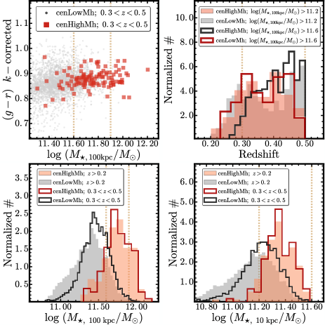
Figure 5: Top-left: The $\log_{10}(M_{\star}/M_{\odot})$-$g-r$ colour relation of the cenHighMh (red circle) and cenLowMh (grey dots) samples. We apply the $k$-corrections from iSEDFit fitting to the colours.   Top-right: the histograms of the redshift for the cenHighMh and cenLowMh galaxies in both $\log_{10}(M_{\star,100\mathrm{kpc}}/M_{\odot})$$>11.2$ and $11.6<$$\log_{10}(M_{\star,100\mathrm{kpc}}/M_{\odot})$$<11.9$ mass bins. The vertical lines highlights the $0.3\leq z\leq 0.5$ redshift range.   Bottom-left: the histograms of $M_{\star,100\mathrm{kpc}}$ for the cenHighMh (orange-red) and cenLowMh (grey-black) samples at both $z>0.2$ (step-filled histogram) and $0.3\leq z\leq 0.5$ (stepped histogram). The vertical lines in both top-left and bottom-left figures highlight the $11.6<$$\log_{10}(M_{\star,100\mathrm{kpc}}/M_{\odot})$$<11.9$ mass range that will be used in the comparison of the $M_{\star,100\mathrm{kpc}}$-matched samples.   Bottom-right: the histograms of $M_{\star,10\mathrm{kpc}}$ in similar format. Here the vertical lines highlight the $11.2<$$\log_{10}(M_{\star,10\mathrm{kpc}}/M_{\odot})$$<11.6$ mass range that is used for comparison.

On the top-left panel of Fig 5, we show the $M_{\star,100\mathrm{kpc}}$-colour relations using the $k$-corrected $g-r$ colour. Both samples follow the same tight ‘red-sequence’ with little contamination from the ‘blue cloud’. At fixed $M_{\star,100\mathrm{kpc}}$, we see little offset in colour distributions of the two samples, suggesting that both samples consist of quiescent galaxies with similar average stellar population properties. This is consistent with previous result that suggests the average stellar population of massive central galaxy does not depend on $M_{\mathrm{200b}}$ (e.g. Park et al. 2007). In this work, we focus on the $M_{\star}$ range of $11.6\leq$$\log_{10}(M_{\star,100\mathrm{kpc}}/M_{\odot})$$\leq 11.9$, where both samples have acceptable completeness, and their $M_{\star,100\mathrm{kpc}}$ distributions greatly overlap (see the normalized distributions of $M_{\star,100\mathrm{kpc}}$ in the bottom-left panel of Fig 5). As for the $M_{\star,10\mathrm{kpc}}$ distributions, the two samples overlap the most within $11.2\leq$$\log_{10}(M_{\star,100\mathrm{kpc}}/M_{\odot})$$\leq 11.6$, but now they show quite different distributions (bottom-right figure).

The redshift distributions also show small difference (upper-right panel) even in the high-$M_{\star,100\mathrm{kpc}}$ bin, where the redshift distribution of the cenLowMh sample skews toward higher-$z$ end due to the contribution of BOSS spec-$z$. Since this could bias the comparison of $\mu_{\star}$ profiles and other properties (please see AppendixB for more details), we address this via matching the two samples in both mass and redshift distributions carefully (see Appendix C).

Appendix B Comparisons of $\mu_{\star}$ profiles in different redshift bins

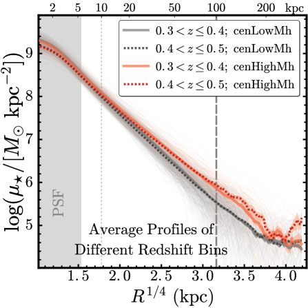
Figure 6: Comparison of $\mu_{\star}$ profiles of cenHighMh (orange-red) and cenLowMh (grey-black) at $11.6\leq$$\log_{10}(M_{\star,100\mathrm{kpc}}/M_{\odot})$$<11.9$ in redshift bins of $0.3\leq z<0.4$ (solid lines) and $0.4\leq z<0.5$ (dash lines). We show the individual profile in the background using much thinner line, and highlight the median profiles using thicker line and darker colour.

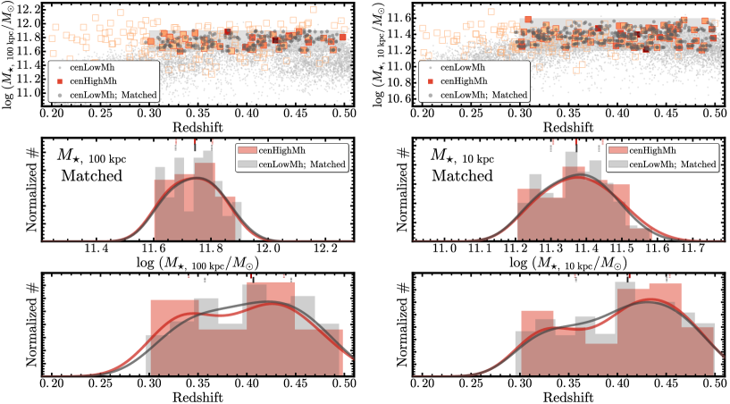
Figure 7: Left figure shows the details of the $M_{\star,100\mathrm{kpc}}$-matching process, corresponding to the results shown in the left figure of On the top panel, we show the overall distributions of cenHighMh (light orange boxes) and cenLowMh (light grey dots) galaxies on the $M_{\star,100\mathrm{kpc}}$-$z$ plane. And, we match the two sample in the $M_{\star,100\mathrm{kpc}}$-$z$ space outlined by the shaded region. We highlight the cenHighMh galaxies in this region using bigger boxes in red frames, whose size reflects the $P_{\mathrm{Cen}}$ value. We also colour-code them using the richness ($\lambda$) of the host cluster. The matched cenLowMh galaxies are highlighted using darker colour and bigger dots. To further evaluate the matching results, we show the distributions of $M_{\star,100\mathrm{kpc}}$ (middle panel) and redshift (bottom panel) separately. On both panels, we show the histograms along with their kernel density distributions. And, on the top of each panel, two sets of short vertical lines highlight the median value (solid) and the inter-quartile (dash) of each distribution.    Right figure shows the similar matching results for the $M_{\star,10\mathrm{kpc}}$-matched samples used for the right figure of Fig 2. The format is exactly the same as the left one, except the $M_{\star,10\mathrm{kpc}}$ replaces the $M_{\star,100\mathrm{kpc}}$ in the top and middle panels.

Given the redshift range for our samples, it is important to evaluate the impacts from the physical extend of seeing and the imaging depth on the $\mu_{\star}$ profiles at different redshift. Under the same seeing, the $\mu_{\star}$ profile of galaxy at higher-$z$ is more vulnerable to the PSF smearing effect at the center. It is also harder to reach to the same $\mu_{\star}$ level under the same imaging depth due to cosmological dimming and background noise.

In Fig 6, we group the cenHighMh and cenLowMh galaxies within $11.6\leq$$\log_{10}(M_{\star,100\mathrm{kpc}}/M_{\odot})$$<11.9$ into two $z$ bins ($0.3\leq z<0.4$ and $0.4\leq z<0.5$), and compare their $\mu_{\star}$ profiles. In two redshift bins, the median $\mu_{\star}$ profiles from the same sample follow each other very well outside 10 kpc, but become visibly different in the central 3-4 kpc, where the effect from seeing kicks in. Meanwhile, the median $\mu_{\star}$ profiles of cenHighMh and cenLowMh in the same $z$ bin are identical in the central region, which indicates similar average seeing conditions. This confirms that $\mu_{\star}$ profile at $>5$ kpc is safe from the impacts of seeing and difference in redshift. More importantly, it also suggests that, once the redshift distributions are carefully matched, the difference of $\mu_{\star}$ profile is likely to be physical even in the central region.

Appendix C Match the cenHighMh and cenLowMh samples in $M_{\star}$ and redshift distributions

As explained earlier, it is important to make sure the two samples have similar distributions in both $M_{\star}$ and redshift before comparing their median $\mu_{\star}$ profiles. Here we briefly describe the procedure used in this work. Since the cenHighMh sample is smaller in size, we always match the cenLowMh sample to it by searching for the $N$-nearest neighbours on the $M_{\star}$-redshift plane using the KDTree algorithm in the scikit-learn Python library (Pedregosa et al. 2011), and evaluate the quality of the match using the distributions of both parameters (as shown in Fig 7).

As we only keep the unique cenLowMh galaxies in the matched sample, we manually adjust the value of $N$ to achieve the best match. When the redshift distribution of the cenHighMh sample becomes bi-model, we also try to split the sample into two redshift bins and match them separately. Typically $N$ is between 3 to 8. In Fig 7, we demonstrate this procedure using the results for the $M_{\star,100\mathrm{kpc}}$-matched (Left) and the $M_{\star,10\mathrm{kpc}}$-matched samples in Fig 2 (Right), and the two samples are well matched in the distributions of $M_{\star,100\mathrm{kpc}}$ (or $M_{\star,10\mathrm{kpc}}$) and redshift. For all the comparisons of $\mu_{\star}$ profiles in this work, we match the samples in the same way, and make sure the match has the same quality.

Appendix D Robustness of the $\mu_{\star}$ Differences

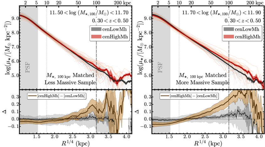
Figure 8: Comparisons of the $\mu_{\star}$ profiles for $M_{\star,100\mathrm{kpc}}$-matched cenHighMh (orange-red) and cenLowMh (grey-black) galaxies in lower (left; [11.5,11.70]) and higher (right; [11.7, 11.9]) $M_{\star,100\mathrm{kpc}}$ bins. Other formats are in consistent with the right figure of Fig 2. The difference in median profiles is more significant in higher $M_{\star,100\mathrm{kpc}}$ bin.

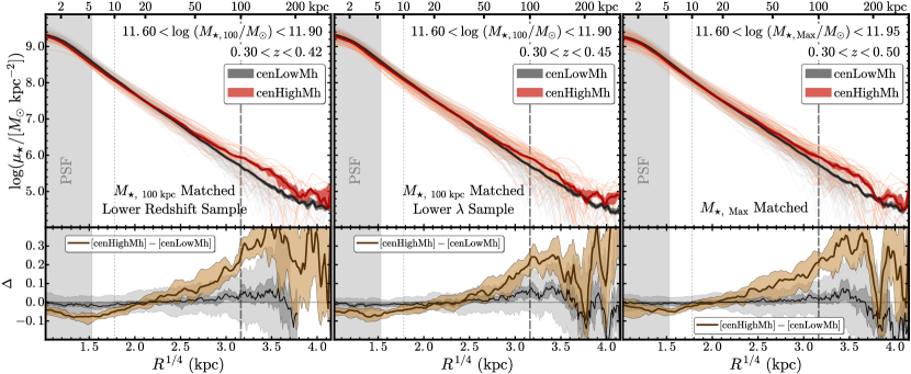
Figure 9: Comparisons of the $\mu_{\star}$ profiles for cenHighMh (orange-red) and cenLowMh (grey-black) galaxies that are matched using proxies of total $M_{\star}$. The formats are in consistent with the right figure of Fig 2. The differences are, here, the samples are matched in slightly different ways. From left to right: a) using samples at lower redshift ($0.3<z<0.4$); b) using cenHighMh sample with $\lambda>20$ instead of 30; c) using $M_{\star}$ within 150 kpc instead of 100 kpc. The results are broadly consistent with the one in Fig 2.

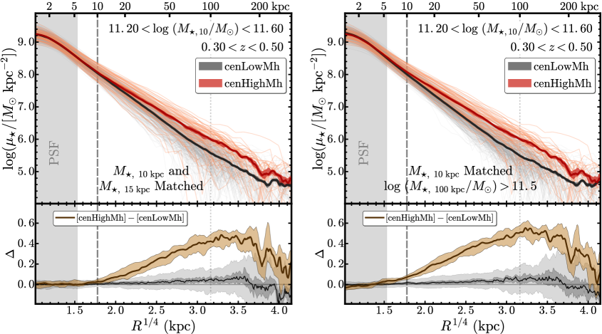
Figure 10: Comparisons of the $\mu_{\star}$ profiles for cenHighMh (orange-red) and cenLowMh (grey-black) galaxies that are matched using the $M_{\star}$ enclosed in the inner region. Left panel shows the results after matching the $M_{\star,10\mathrm{kpc}}$ and $M_{\star,15\mathrm{kpc}}$ together, and the right panel shows the results when only the $\log_{10}(M_{\star,100\mathrm{kpc}}/M_{\odot})$$\geq 11.5$ cenHighMh and cenLowMh galaxies are included. Other formats are in consistent with the right figure of Fig 2.

In Fig 2, we compare the $\mu_{\star}$ profiles of $M_{\star,100\mathrm{kpc}}$- and $M_{\star,10\mathrm{kpc}}$-matched samples of cenHighMh and cenLowMh galaxies, and here we test the robustness of the results using a few extra tests that are illustrated in Fig 8, Fig 9, and Fig 10, and are briefly described here:

1. In Fig 8, we group the samples into two $M_{\star,100\mathrm{kpc}}$ bins. Given the small sample size, we extend slightly toward lower $M_{\star,100\mathrm{kpc}}$ range ($11.5\leq\log_{10}(M_{\star,\ 10\mathrm{kpc}}/M_{\odot})<11.7$ and $11.7\leq\log_{10}(M_{\star,\ 10\mathrm{kpc}}/M_{\odot})<11.9$). Although the smaller sample leads to larger statistical uncertainties, we can still see similar structural differences in both $M_{\star,100\mathrm{kpc}}$ bins, and the difference becomes more significant in the higher $M_{\star,100\mathrm{kpc}}$ bin. For the lower $M_{\star,100\mathrm{kpc}}$ bin, the difference in the inner region becomes quite uncertain, while the difference in the outskirt is still visible. This potentially suggests that the environmental dependence of structure also varies with $M_{\star}$, an important implication deserves more investigations in the future.

2. On the left panel of Fig 9, we match the cenHighMh and cenLowMh samples in a lower redshift bins ($0.30<z<0.42$). Despite the larger uncertainties due to smaller samples, we find the results are the same.

3. On the middle panel of Fig 9, we includes cenHighMh galaxies in poorer clusters ($20<\lambda<30$), which should result in overlapped $M_{\mathrm{200b}}$ distributions with the cenLowMh samples considering the typical uncertainty of $\lambda$. This makes the difference in the inner region slightly less significant, but the overall results are the same.

4. On the right panel of Fig 9, in stead of using $M_{\star,100\mathrm{kpc}}$, we use the $M_{\star,\mathrm{Max}}$–the maximum $M_{\star}$ by integrating the $\mu_{\star}$ profiles to the largest radius allowed. The $M_{\star,\mathrm{Max}}$ values are less reliable than $M_{\star,100\mathrm{kpc}}$ due to the uncertainty of background subtraction and contamination from nearby bright objects, but they can serve as different estimates of the ‘total’ $M_{\star}$ of these galaxies. As shown in § 4, they on average increase the $M_{\star}$ by a little bit and affect the cenHighMh more. The differences in the $\mu_{\star}$ profiles still remain very similar.

We also test the robustness of the $M_{\star,100\mathrm{kpc}}$-matched results using the samples with only spectroscopic redshift, the samples in the three GAMA fields, and the cenHighMh samples without the ones in very massive haloes ($\lambda>40$). Limited by space, we do not show these results here, but they all verify the robustness of the results.

For the results from the $M_{\star,10\mathrm{kpc}}$-matched samples:

1. We match the two samples using both $M_{\star,10\mathrm{kpc}}$ and the $M_{\star}$ within 15 kpc at the same time. This makes the two median $\mu_{\star}$ profiles very similar inside 10-15 kpc, while the result in the outskirt remains the same (left panel of Fig 10). Use $M_{\star}$ within 5 or 20 kpc leads to the same conclusion.

2. To make sure the two samples are comparable in their overall assembly history, we also try to only include the very massive galaxies ($\log_{10}(M_{\star,100\mathrm{kpc}}/M_{\odot})$$>11.5$) in both samples. This excludes the cenLowMh galaxies that are much less massive and more ‘compact’ in structure. Yet, the results regarding the structural differences remain the same.

Appendix E Stellar Mass Curve-of-Growth for Massive Central Galaxies

In §3.1 and Figure 2, we show the comparisons of $\mu_{\star}$ profiles for massive central galaxies from the cenHighMh and cenLowMh samples. Although the differences in their median $\mu_{\star}$ profiles we revealed are robust and systematic, they appear to be very subtle, especially in the inner region. This is partly due to the logarithmic scale on the Y–axis for $\mu_{\star}$ profiles.

In Figure 12, we compare the same two samples after converting the $\mu_{\star}$ profiles into:

1. ‘Curve-of-growth’ of stellar mass – the cumulative $\log_{10}(M_{\star}/M_{\odot})$ profiles (upper panel).

2. Fraction of $M_{\star,100\mathrm{kpc}}$ within different radius (lower panel).

These comparisons demonstrate the same results from different angles and the systematic differences become more clear using the fraction of $M_{\star,100\mathrm{kpc}}$ within different radius. The comparison of cumulative $\log_{10}(M_{\star}/M_{\odot})$ profiles also demonstrates that the cenHighMh and cenLowMh samples have very similar median $M_{\star,100\mathrm{kpc}}$. They help confirm that the distributions of stellar mass within 100 kpc indeed have systematic differences between the massive central galaxies living in more and less massive dark matter haloes.

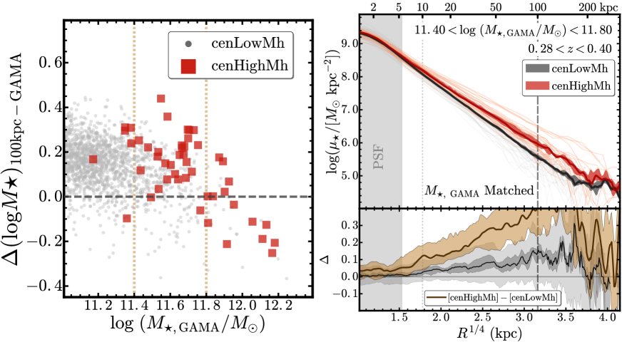
Figure 11: Left: comparison of $M_{\star}$ estimated by the GAMA survey and the $M_{\star,100\mathrm{kpc}}$ using HSC images in this work. We plot the $\log_{10}(M_{\star,\mathrm{GAMA}}/M_{\odot})$ against the difference between $\log_{10}(M_{\star,100\mathrm{kpc}}/M_{\odot})$ and $\log_{10}(M_{\star,\mathrm{GAMA}}/M_{\odot})$. The two vertical lines highlight the mass range $11.4\leq$$\log_{10}(M_{\star,\mathrm{GAMA}}/M_{\odot})$$<11.8$ that is used for the comparison.   Right: we compare the $\mu_{\star}$ profiles of cenHighMh (orange-red) and cenLowMh (grey-black) galaxies using the samples matched on the $M_{\star,\mathrm{GAMA}}$-$z$ plane at $11.4\leq$$\log_{10}(M_{\star,\mathrm{GAMA}}/M_{\odot})$$<11.9$ and $0.28\leq z<0.4$. The format is very similar to the ones in Fig 2.

Appendix F Comparison of $\mu_{\star}$ profiles using $M_{\star}$ from the GAMA survey

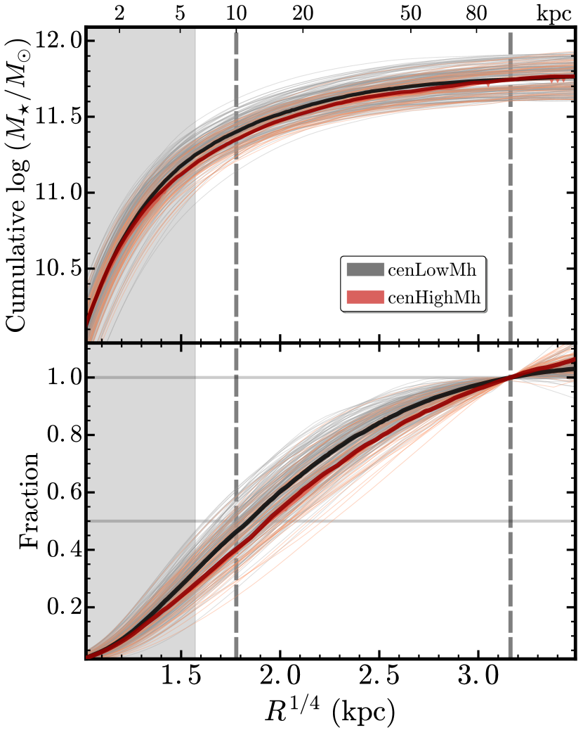
Figure 12: Top: comparison of the cumulative $M_{\star}$ profiles for cenHighMh (orange–red) and cenLowMh (grey–black) galaxies at fixed $M_{\star,100\mathrm{kpc}}$.   Bottom: comparison of the fraction of $M_{\star,100\mathrm{kpc}}$ within different radius for the same samples at fixed $M_{\star,100\mathrm{kpc}}$. Thicker and darker solid lines highlight the median profiles. Other formats of the figure are similar to Figure 2. Besides the region affected by seeing, the 10 and 100 kpc radius, we also highlight the 50% and 100% values using horizontal grey lines on the bottom panel.

The GAMA survey greatly overlaps with the HSC survey, and it provides carefully measured $M_{\star}$ for large sample of galaxies (Taylor et al. 2011) that help produce many interesting results (e.g., Bauer et al. 2013; Ferreras et al. 2017). They use 2-D single-Sérsic  model to correct the total luminosity of the galaxy (Kelvin et al. 2012), and derive the $M_{\star}/L_{\star}$ through optical-SED fitting (BC03 model; Chabrier IMF) based on the PSF-matched aperture photometry. Since the Sérsic  model is generally more flexible than the cModel one, it is therefore interesting to compare with the cenHighMh and cenLowMh galaxies that also have spec-$z$ (at $z<0.40$) and $M_{\star}$ in GAMA DR2 (Liske et al. 2015) and see the impact of deep photometry again.

We summarize the results in Fig 11. On the left panel, we compare the differences between $M_{\star,100\mathrm{kpc}}$ and $M_{\star,\mathrm{GAMA}}$. HSC survey on average recovers more $M_{\star}$ at high-$M_{\star}$ end, which is consistent with the expectation from deeper photometry, although the systematic differences in the estimates of $M_{\star}/L_{\star}$ could play a role here. Meanwhile, it is interesting see that, above $\log_{10}(M_{\star,100\mathrm{kpc}}/M_{\odot})$$>11.8$, $M_{\star,\mathrm{GAMA}}$ becomes increasingly larger than $M_{\star,100\mathrm{kpc}}$, and most of these massive galaxies have very high Sérsic  index from the 2-D fitting. This suggests that the single-Sérsic  model is no longer an appropriate one to describe very massive galaxies as it tends to over-estimate the $M_{\star}$ the inner and/or outer regions.

To verify the cause of the difference in $M_{\star}$, we further select samples of cenHighMh and cenLowMh galaxies with matched $M_{\star,\mathrm{GAMA}}$ and redshift distributions (at $11.4<$$\log_{10}(M_{\star,\mathrm{GAMA}}/M_{\odot})$$<11.8$; see Appendix C), and compare their $\mu_{\star}$ profiles (right panel). Although these two subsamples are equally massive according to results from GAMA survey, it is clear that the cenHighMh galaxy has much more extended outer envelope, even though its median $\mu_{\star}$ profile is very similar to the cenLowMh sample at $<10$ kpc. We can reproduce very the same trend with the luminosity density profiles (with or without $k$-correction), suggesting that the inaccurate Sérsic  model definitely leads to under-estimate of $M_{\star}$.

References

- Abazajian et al. (2009) Abazajian K. N., et al., 2009, ApJS, 182, 543
- Aihara et al. (2011) Aihara H., et al., 2011, ApJS, 193, 29
- Aihara et al. (2017b) Aihara H., et al., 2017b, preprint, (arXiv:1702.08449)
- Aihara et al. (2017a) Aihara H., et al., 2017a, preprint, (arXiv:1704.05858)
- Alam et al. (2015) Alam S., et al., 2015, ApJS, 219, 12
- Allen et al. (2015) Allen R. J., et al., 2015, ApJ, 806, 3
- Astropy Collaboration et al. (2013) Astropy Collaboration et al., 2013, A&A, 558, A33
- Axelrod et al. (2010) Axelrod T., Kantor J., Lupton R. H., Pierfederici F., 2010, in Software and Cyberinfrastructure for Astronomy. p. 774015, doi:10.1117/12.857297
- Barbary et al. (2015) Barbary Boone Deil 2015, sep: v0.3.0, doi:10.5281/zenodo.15669, http://dx.doi.org/10.5281/zenodo.15669
- Barbosa et al. (2016) Barbosa C. E., Arnaboldi M., Coccato L., Hilker M., Mendes de Oliveira C., Richtler T., 2016, A&A, 589, A139
- Bassett et al. (2013) Bassett R., et al., 2013, ApJ, 770, 58
- Bauer et al. (2013) Bauer A. E., et al., 2013, MNRAS, 434, 209
- Bédorf & Portegies Zwart (2013) Bédorf J., Portegies Zwart S., 2013, MNRAS, 431, 767
- Behroozi et al. (2013) Behroozi P. S., Wechsler R. H., Conroy C., 2013, ApJ, 770, 57
- Belli et al. (2015) Belli S., Newman A. B., Ellis R. S., 2015, ApJ, 799, 206
- Bernardi et al. (2010) Bernardi M., Shankar F., Hyde J. B., Mei S., Marulli F., Sheth R. K., 2010, MNRAS, 404, 2087
- Bernardi et al. (2014) Bernardi M., Meert A., Vikram V., Huertas-Company M., Mei S., Shankar F., Sheth R. K., 2014, MNRAS, 443, 874
- Bonfini & Graham (2016) Bonfini P., Graham A. W., 2016, ApJ, 829, 81
- Bosch et al. (2017) Bosch J., et al., 2017, preprint, (arXiv:1705.06766)
- Boylan-Kolchin & Ma (2007) Boylan-Kolchin M., Ma C.-P., 2007, MNRAS, 374, 1227
- Buchan & Shankar (2016) Buchan S., Shankar F., 2016, MNRAS, 462, 2001
- Buitrago et al. (2017) Buitrago F., Trujillo I., Curtis-Lake E., Montes M., Cooper A. P., Bruce V. A., Pérez-González P. G., Cirasuolo M., 2017, MNRAS, 466, 4888
- Calzetti et al. (2000) Calzetti D., Armus L., Bohlin R. C., Kinney A. L., Koornneef J., Storchi-Bergmann T., 2000, ApJ, 533, 682
- Cappellari (2013) Cappellari M., 2013, ApJ, 778, L2
- Carlberg et al. (1997) Carlberg R. G., Yee H. K. C., Ellingson E., 1997, ApJ, 478, 462
- Carollo et al. (2013) Carollo C. M., et al., 2013, ApJ, 773, 112
- Cebrián & Trujillo (2014) Cebrián M., Trujillo I., 2014, MNRAS, 444, 682
- Chabrier (2003) Chabrier G., 2003, PASP, 115, 763
- Charlton et al. (2017) Charlton P. J. L., Hudson M. J., Balogh M. L., Khatri S., 2017, preprint, (arXiv:1707.04924)
- Cimatti et al. (2008) Cimatti A., et al., 2008, A&A, 482, 21
- Coccato et al. (2010) Coccato L., Gerhard O., Arnaboldi M., 2010, MNRAS, 407, L26
- Coccato et al. (2011) Coccato L., Gerhard O., Arnaboldi M., Ventimiglia G., 2011, A&A, 533, A138
- Conroy & Gunn (2010a) Conroy C., Gunn J. E., 2010a, FSPS: Flexible Stellar Population Synthesis, Astrophysics Source Code Library (ascl:1010.043)
- Conroy & Gunn (2010b) Conroy C., Gunn J. E., 2010b, ApJ, 712, 833
- D’Souza et al. (2014) D’Souza R., Kauffman G., Wang J., Vegetti S., 2014, MNRAS, 443, 1433
- Damjanov et al. (2009) Damjanov I., et al., 2009, ApJ, 695, 101
- Dekel et al. (2009) Dekel A., Sari R., Ceverino D., 2009, ApJ, 703, 785
- Delaye et al. (2014) Delaye L., et al., 2014, MNRAS, 441, 203
- Diemer (2015) Diemer B., 2015, Colossus: COsmology, haLO, and large-Scale StrUcture toolS, Astrophysics Source Code Library (ascl:1501.016)
- Diemer & Kravtsov (2015) Diemer B., Kravtsov A. V., 2015, ApJ, 799, 108
- Fagioli et al. (2016) Fagioli M., Carollo C. M., Renzini A., Lilly S. J., Onodera M., Tacchella S., 2016, ApJ, 831, 173
- Fan et al. (2008) Fan L., Lapi A., De Zotti G., Danese L., 2008, ApJ, 689, L101
- Farahi et al. (2016) Farahi A., Evrard A. E., Rozo E., Rykoff E. S., Wechsler R. H., 2016, MNRAS, 460, 3900
- Ferreras et al. (2017) Ferreras I., et al., 2017, Galaxy and Mass Assembly (GAMA): Probing the merger histories of massive galaxies via stellar populations (arXiv:1703.00465)
- Foreman-Mackey et al. (2013) Foreman-Mackey D., Hogg D. W., Lang D., Goodman J., 2013, PASP, 125, 306
- Genel et al. (2017) Genel S., et al., 2017, preprint, (arXiv:1707.05327)
- Gonzalez et al. (2005) Gonzalez A. H., Zabludoff A. I., Zaritsky D., 2005, ApJ, 618, 195
- Greene et al. (2015) Greene J. E., Janish R., Ma C.-P., McConnell N. J., Blakeslee J. P., Thomas J., Murphy J. D., 2015, ApJ, 807, 11
- Guo et al. (2009) Guo Y., et al., 2009, MNRAS, 398, 1129
- Guo et al. (2011) Guo Q., et al., 2011, MNRAS, 413, 101
- Heymans et al. (2012) Heymans C., et al., 2012, MNRAS, 427, 146
- Hill et al. (2017) Hill A. R., et al., 2017, ApJ, 837, 147
- Hilz et al. (2013) Hilz M., Naab T., Ostriker J. P., 2013, MNRAS, 429, 2924
- Hirschmann et al. (2013) Hirschmann M., De Lucia G., Iovino A., Cucciati O., 2013, MNRAS, 433, 1479
- Hopkins et al. (2008) Hopkins P. F., Hernquist L., Cox T. J., Dutta S. N., Rothberg B., 2008, ApJ, 679, 156
- Hoshino et al. (2015) Hoshino H., et al., 2015, MNRAS, 452, 998
- Huang et al. (2013a) Huang S., Ho L. C., Peng C. Y., Li Z.-Y., Barth A. J., 2013a, ApJ, 766, 47
- Huang et al. (2013b) Huang S., Ho L. C., Peng C. Y., Li Z.-Y., Barth A. J., 2013b, ApJ, 768, L28
- Huang et al. (2017) Huang S., Leauthaud A., Greene J., Bundy K., Lin Y.-T., Tanaka M., Miyazaki S., Komiyama Y., 2017, preprint, (arXiv:1707.01904)
- Huertas-Company et al. (2013) Huertas-Company M., Shankar F., Mei S., Bernardi M., Aguerri J. A. L., Meert A., Vikram V., 2013, ApJ, 779, 29
- Hunter (2007) Hunter J. D., 2007, Computing In Science & Engineering, 9, 90
- Jones et al. (2001) Jones E., Oliphant T., Peterson P., et al., 2001, SciPy: Open source scientific tools for Python, http://www.scipy.org/
- Jurić et al. (2015) Jurić M., et al., 2015, preprint, (arXiv:1512.07914)
- Keating et al. (2015) Keating S. K., Abraham R. G., Schiavon R., Graves G., Damjanov I., Yan R., Newman J., Simard L., 2015, ApJ, 798, 26
- Kelkar et al. (2015) Kelkar K., Aragón-Salamanca A., Gray M. E., Maltby D., Vulcani B., De Lucia G., Poggianti B. M., Zaritsky D., 2015, MNRAS, 450, 1246
- Kelvin et al. (2012) Kelvin L. S., et al., 2012, MNRAS, 421, 1007
- Khochfar & Silk (2006) Khochfar S., Silk J., 2006, ApJ, 648, L21
- Kuchner et al. (2017) Kuchner U., Ziegler B., Verdugo M., Bamford S., Häußler B., 2017, preprint, (arXiv:1705.03839)
- La Barbera et al. (2010) La Barbera F., De Carvalho R. R., De La Rosa I. G., Gal R. R., Swindle R., Lopes P. A. A., 2010, AJ, 140, 1528
- La Barbera et al. (2012) La Barbera F., Ferreras I., de Carvalho R. R., Bruzual G., Charlot S., Pasquali A., Merlin E., 2012, MNRAS, 426, 2300
- Lani et al. (2013) Lani C., et al., 2013, MNRAS, 435, 207
- Leauthaud et al. (2012) Leauthaud A., et al., 2012, ApJ, 744, 159
- Leja et al. (2013) Leja J., van Dokkum P., Franx M., 2013, ApJ, 766, 33
- Lin & Mohr (2004) Lin Y.-T., Mohr J. J., 2004, ApJ, 617, 879
- Liske et al. (2015) Liske J., et al., 2015, MNRAS, 452, 2087
- López-Cruz et al. (2014) López-Cruz O., Añorve C., Birkinshaw M., Worrall D. M., Ibarra-Medel H. J., Barkhouse W. A., Torres-Papaqui J. P., Motta V., 2014, ApJ, 795, L31
- Maltby et al. (2010) Maltby D. T., et al., 2010, MNRAS, 402, 282
- Mandelbaum et al. (2018) Mandelbaum R., et al., 2018, PASJ, 70, S25
- Martizzi et al. (2013) Martizzi D., Teyssier R., Moore B., 2013, MNRAS, 432, 1947
- McCarthy et al. (2017) McCarthy I. G., Schaye J., Bird S., Le Brun A. M. C., 2017, MNRAS, 465, 2936
- Melchior et al. (2016) Melchior P., et al., 2016, preprint, (arXiv:1610.06890)
- Mihos et al. (2005) Mihos J. C., Harding P., Feldmeier J., Morrison H., 2005, ApJ, 631, L41
- Milosavljević et al. (2002) Milosavljević M., Merritt D., Rest A., van den Bosch F. C., 2002, MNRAS, 331, L51
- Miyazaki et al. (2012) Miyazaki S., et al., 2012, in Ground-based and Airborne Instrumentation for Astronomy IV. p. 84460Z, doi:10.1117/12.926844
- Moustakas et al. (2013) Moustakas J., et al., 2013, ApJ, 767, 50
- Murata et al. (2017) Murata R., Nishimichi T., Takada M., Miyatake H., Shirasaki M., More S., Takahashi R., Osato K., 2017, preprint, (arXiv:1707.01907)
- Naab et al. (2006) Naab T., Khochfar S., Burkert A., 2006, ApJ, 636, L81
- Nair et al. (2010) Nair P. B., van den Bergh S., Abraham R. G., 2010, ApJ, 715, 606
- Newman et al. (2012) Newman A. B., Ellis R. S., Bundy K., Treu T., 2012, ApJ, 746, 162
- Oh et al. (2017) Oh S., Greene J. E., Lackner C. N., 2017, ApJ, 836, 115
- Oke & Gunn (1983) Oke J. B., Gunn J. E., 1983, ApJ, 266, 713
- Oogi & Habe (2013) Oogi T., Habe A., 2013, MNRAS, 428, 641
- Oser et al. (2010) Oser L., Ostriker J. P., Naab T., Johansson P. H., Burkert A., 2010, ApJ, 725, 2312
- Oser et al. (2012) Oser L., Naab T., Ostriker J. P., Johansson P. H., 2012, ApJ, 744, 63
- Papovich et al. (2012) Papovich C., et al., 2012, ApJ, 750, 93
- Park et al. (2007) Park C., Choi Y.-Y., Vogeley M. S., Gott III J. R., Blanton M. R., SDSS Collaboration 2007, ApJ, 658, 898
- Patel et al. (2013) Patel S. G., et al., 2013, ApJ, 766, 15
- Pedregosa et al. (2011) Pedregosa F., et al., 2011, Journal of Machine Learning Research, 12, 2825
- Pérez & Granger (2007) Pérez F., Granger B. E., 2007, Computing in Science and Engineering, 9, 21
- Pillepich et al. (2017) Pillepich A., et al., 2017, preprint, (arXiv:1707.03406)
- Poggianti et al. (2013) Poggianti B. M., Moretti A., Calvi R., D’Onofrio M., Valentinuzzi T., Fritz J., Renzini A., 2013, ApJ, 777, 125
- Postman et al. (2012) Postman M., et al., 2012, ApJ, 756, 159
- Price et al. (2017) Price S. H., Kriek M., Feldmann R., Quataert E., Hopkins P. F., Faucher-Giguère C.-A., Kereš D., Barro G., 2017, preprint, (arXiv:1707.01094)
- Raichoor et al. (2012) Raichoor A., et al., 2012, ApJ, 745, 130
- Reid et al. (2014) Reid B. A., Seo H.-J., Leauthaud A., Tinker J. L., White M., 2014, MNRAS, 444, 476
- Rettura et al. (2010) Rettura A., et al., 2010, ApJ, 709, 512
- Rodriguez-Gomez et al. (2016) Rodriguez-Gomez V., et al., 2016, MNRAS, 458, 2371
- Rozo et al. (2015) Rozo E., Rykoff E. S., Becker M., Reddick R. M., Wechsler R. H., 2015, MNRAS, 453, 38
- Rykoff et al. (2014) Rykoff E. S., et al., 2014, ApJ, 785, 104
- Saito et al. (2016) Saito S., et al., 2016, MNRAS, 460, 1457
- Saro et al. (2015) Saro A., et al., 2015, MNRAS, 454, 2305
- Schlafly & Finkbeiner (2011) Schlafly E. F., Finkbeiner D. P., 2011, ApJ, 737, 103
- Shankar et al. (2013) Shankar F., Marulli F., Bernardi M., Mei S., Meert A., Vikram V., 2013, MNRAS, 428, 109
- Shankar et al. (2014) Shankar F., et al., 2014, MNRAS, 439, 3189
- Shankar et al. (2015) Shankar F., et al., 2015, ApJ, 802, 73
- Shen et al. (2003) Shen S., Mo H. J., White S. D. M., Blanton M. R., Kauffmann G., Voges W., Brinkmann J., Csabai I., 2003, MNRAS, 343, 978
- Simet et al. (2017) Simet M., McClintock T., Mandelbaum R., Rozo E., Rykoff E., Sheldon E., Wechsler R. H., 2017, MNRAS, 466, 3103
- Sonnenfeld & Leauthaud (2017) Sonnenfeld A., Leauthaud A., 2017, preprint, (arXiv:1710.00007)
- Strazzullo et al. (2013) Strazzullo V., et al., 2013, ApJ, 772, 118
- Szomoru et al. (2012) Szomoru D., Franx M., van Dokkum P. G., 2012, ApJ, 749, 121
- Tal & van Dokkum (2011) Tal T., van Dokkum P. G., 2011, ApJ, 731, 89
- Taylor et al. (2011) Taylor E. N., et al., 2011, MNRAS, 418, 1587
- Thomas et al. (2016) Thomas J., Ma C.-P., McConnell N. J., Greene J. E., Blakeslee J. P., Janish R., 2016, Nature, 532, 340
- Trujillo et al. (2006) Trujillo I., et al., 2006, MNRAS, 373, L36
- Vanderplas et al. (2012) Vanderplas J., Connolly A., Ivezić Ž., Gray A., 2012, in Conference on Intelligent Data Understanding (CIDU). pp 47 –54, doi:10.1109/CIDU.2012.6382200
- Walt et al. (2011) Walt S. v. d., Colbert S. C., Varoquaux G., 2011, Computing in Science and Engg., 13, 22
- Weinmann et al. (2009) Weinmann S. M., Kauffmann G., van den Bosch F. C., Pasquali A., McIntosh D. H., Mo H., Yang X., Guo Y., 2009, MNRAS, 394, 1213
- Yoon et al. (2017) Yoon Y., Im M., Kim J.-W., 2017, ApJ, 834, 73
- van Dokkum et al. (2008) van Dokkum P. G., et al., 2008, ApJ, 677, L5
- van Dokkum et al. (2010) van Dokkum P. G., et al., 2010, ApJ, 709, 1018
- van Uitert et al. (2016) van Uitert E., et al., 2016, MNRAS, 459, 3251
- van der Wel et al. (2011) van der Wel A., et al., 2011, ApJ, 730, 38
- van der Wel et al. (2014) van der Wel A., et al., 2014, ApJ, 788, 28