New Experimental Limits on Exotic Spin-Spin-Velocity-Dependent Interactions By Using SmCo₅ Spin Sources

Abstract

We report the latest results of searching for possible new macro-scale spin-spin-velocity-dependent forces (SSVDFs) based on specially designed iron-shielded SmCo₅ (ISSC) spin sources and a spin exchange relaxation free (SERF) co-magnetometer. The ISSCs have high net electron spin densities of about $1.7\times 10^{21}$ cm^-3, which mean high detecting sensitivity; and low magnetic field leakage of about $\sim$mG level due to iron shielding, which means low detecting noise. With help from the ISSCs, the high sensitivity SERF co-magnetometer, and the similarity analysis method, new constraints on SSVDFs with forms of $V_{6+7}$, $V_{8}$, $V_{15}$, and $V_{16}$ have been obtained, which represent the tightest limits in force range of 5 cm – 1 km to the best of our knowledge.

Introduction–

Many new light bosons, such as axion Wilczek (1978); Weinberg (1978); R.D.Peccei and Quinn (1977), dark photon Jaeckel and Ringwald (1978); An et al. (2015), paraphoton Dobrescu (2005), familon and majoron (C.Patrignani et al., 2016), have been introduced by theories beyond the Standard Model. If they exist, these kinds of new bosons may mediate new types of long-range fundamental forces, or the so-called 5th forces. These possible new forces may break the C, P, or T (or their combinations) symmetry R.D.Peccei and Quinn (1977), and they have been suspected to be answers to questions like the strong CP violation problem R.D.Peccei and Quinn (1977). The possibility of the existence of 5th forces has been extensively investigated experimentally Jaeckel and Ringwald (2010); Hill and Ross (1988). Many forms of technology have been used to search for these long-range spin- and/or velocity-dependent forces, including the torsion balance Ritter et al. (1990); Heckel et al. (2006); Terrano et al. (2015); Hammond et al. (2007), the resonance spring Long et al. (2003); Long and Kostelecký (2015), the spin exchange relaxation free (SERF) co-magnetometer Vasilakis et al. (2009); Heckel et al. (2013); Terrano et al. (2015); Wineland et al. (1991), nuclear magnetic resonance (NMR) based methods Petukhov et al. (2010); Yan et al. (2015); Chu et al. (2013), and other high sensitivity technologies Tullney et al. (2013); Serebrov et al. (2010); Ficek et al. (2017); Fu et al. (2010).

In all of these experiments, in order to increase detecting sensitivities, one of the key issues was how to improve the test matter’s polarized spin density. This is due to the fact that a Yukawa-like force is proportional to $e^{-r/\lambda}$Dobrescu and Mocioiu (2006), where r is the source to probe distance and $\lambda$ is the force range. For small $\lambda$, like in the range of about $1<\lambda<100$ cm, because of the limited volume $O(\lambda^{3})$ , increasing the polarized spin density is very critical to improve the detecting sensitivity.

It has been pointed out that interactions between two spin-1/2 fermions, which are mediated by spin 0 or spin 1 bosons, could be classified to 16 terms, and 9 of them are spin-spin dependent Dobrescu and Mocioiu (2006). Among the spin-spin dependent terms, 3 of them are static, and 6 of them depend on the relative velocity between two polarized objects. Compared with the static terms Vasilakis et al. (2009); Heckel et al. (2013); Terrano et al. (2015); Wineland et al. (1991); Hunter et al. (2013), the experimental constraints on the spin-spin-velocity-dependent forces (SSVDFs) are still rare today Hunter and Ang (2014); Ficek et al. (2017). For the latter terms, not only a relative velocity between the source and the probe is required, but also both of them must be spin-polarized. Therefore, they are more difficult to study experimentally.

In Ref. Ji et al. (2017), an experimental scheme with high electron spin-density sources, iron-shielded SmCo₅ (ISSCs), was proposed to detect the SSVDFs. By taking advantage of the high electron spin density of ISSC and the high sensitivity of SERF co-magnetometer Kornack et al. (2005), the proposed system had a potential to detect several SSVDFs with record sensitivities. In this letter, we report new experimental studies on the SSVDFs by using ISSCs and a SERF co-magnetometer Chen et al. (2016); Fang et al. (2016a, b); Smiciklas et al. (2011).

The SERF’s Response to the SSVDFs–

SSVDFs to be studied here are, following the notation in Ref. Dobrescu and Mocioiu (2006); Leslie et al. (2014), $V_{6+7}$, $V_{8}$, $V_{15}$ and $V_{16}$. For example, $V_{16}$ can be written as,

$$\begin{split}V_{16}=&-\frac{f_{16}\hbar^{2}}{8\pi m_{\mu}c^{2}}\big{\{}(\hat{\bm{\sigma}_{2}}\cdot\mathbf{v})\left[\hat{\bm{\sigma}_{1}}\cdot(\mathbf{v}\times\hat{\bm{r}})\right]\\ &+(\hat{\bm{\sigma}_{1}}\cdot\mathbf{v})\left[\hat{\bm{\sigma}_{2}}\cdot(\mathbf{v}\times\hat{\bm{r}})\right]\big{\}}\left(\frac{1}{\lambda r}+\frac{1}{r^{2}}\right)e^{-r/\lambda},\end{split}$$ (1)

where $f_{16}$ is a dimensionless coupling constant, $\hat{\sigma}_{1}$, $\hat{\sigma}_{2}$ are the spins of the two particles respectively, and $\mathbf{v}$ is the relative velocity between the two interacting fermions. For this new interaction, the corresponding effective magnetic field $\mathbf{B}_{eff}$ experienced by the polarized spin due to the spin source can be deduced from $V_{16}=-\mathbf{\mu}\cdot\mathbf{B}_{eff}$, where $\mu$ is the magnetic momentum of the probing particle. In a typical polarized noble gas experiment, the probe particles could be nuclei, e.g. ²¹Ne, or valence electrons of alkali.

If this $\mathbf{B}_{eff}$ exists, the SERF’s response can be estimated by the Bloch equationsKominis et al. (2003),

$$\frac{\partial\mathbf{P}^{e}}{\partial t}=\frac{\gamma_{e}}{Q(P^{e})}\left[\mathbf{B}_{eff}^{e}+\mathbf{B}+\lambda M^{n}\mathbf{P}^{n}+\mathbf{L}\right]\times\mathbf{P}^{e}+\frac{P_{0}^{e}\hat{\mathbf{z}}-\mathbf{P}^{e}}{T_{e}Q(P^{e})},$$ (2)

$$\frac{\partial\mathbf{P}^{n}}{\partial t}=\gamma_{n}\left[\mathbf{B}_{eff}^{n}+\mathbf{B}+\lambda M^{e}\mathbf{P}^{e}\right]\times\mathbf{P}^{n}+\frac{P_{0}^{n}\hat{\mathbf{z}}-\mathbf{P}^{n}}{\{T_{2n},T_{2n},T_{1n}\}},$$ (3)

where $\mathbf{B}_{eff}^{e,n}$ are the effective magnetic fields due to the possible new SSVDFs coupling to the electron (or nucleon) spin; $\mathbf{P}^{e,n}$ are the polarization of electron or nucleon respectively; $\mathbf{B}$ is the external magnetic field; $T_{e}$, $T_{1n}$, and $T_{2n}$ are the electron spin’s relaxation time, nucleon spin’s longitudinal and transverse relaxation times respectively; $M^{e,n}$ are the magnetization associated with the electron or the nucleon spin; $P_{0}^{e}$ ($P_{0}^{n}$) is the equilibrium polarization of the electron ( nucleon); $\mathbf{L}$ is the pumping light induced effective magnetic field experienced by the electron spin; $Q(P^{e})$ is the electron slow-down factor associated with the hyperfine interaction and spin-exchange collisions Kornack and Romalis (2002); and $\gamma_{e}$ ($\gamma_{n}$) is the gyromagnetic ratio of the electron (nucleon). It is worth noticing that the Eq.(2) and (3) are coupled together. For example, if $B^{n}_{eff}=0$, but $B^{e}_{eff}\neq 0$, the SERF still has nonzero output $S^{sim}(t)$.

By solving the equation set (2) and (3) numerically, one can convert the SERF’s response $\mathbf{P}^{e}(t)$ to a variable field $\mathbf{B}^{e,n}_{eff}$. The numerical results, together with the experimental measurements, are shown in Fig. 1. As shown in Fig. 1, the sensitivity of the co-magnetometer’s response was frequency dependent.

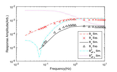
Figure 1: (Color online) SERF’s response to magnetic fields. The red crosses and red dash line are experimental and simulation results for $B_{x}$ respectively, while the black triangles and black solid line are for $B_{y}$. The simulation results were obtained by solving Eq. 2&3 numerically. The pink dot line and blue dash-dot line are simulations with assumptions that the exotic force only affected electrons.

Experimental Setup–

The experiment was carried out at Beihang University, Beijing, China. The setup is shown in Fig. 2 schematically. The left side is a SERF co-magnetometer. A detailed description of the device can be found in Ref. Chen et al. (2016). A spherical aluminosilicate glass vapor cell with a diameter of 14 mm was located at the center of the SERF. It was filled with 3 bar of ²¹Ne gas (isotope enriched to 70$\%$ ), 53 mbar of N₂ gas, and a small amount of K-Rb mixture. The mixture mole ratio was about 0.05 for the hybrid pumping purpose Smiciklas et al. (2011). The cell was shielded by four layers of $\mu$-metal and a layer of 10-mm-thick ferrite Kornack et al. (2007) magnetic field shielding to reduce the ambient magnetic field.

As shown in Fig. 2, a linearly polarized probe laser beam, which was modulated by a 50 kHz signal, passed through the cell, and its Faraday rotation angle was then measured by using photo-elastic modulation (PEM). The signals from photo-diodes were amplified by a lock-in amplifier, which had a reference frequency of 50 kHz, the same as the probe’s modulation. The lock-in output was then recorded by a data-acquisition system.

As shown at the right side in Fig. 2 , there were two ISSCs, the electron spin sources. They were identical iron-shielded SmCo₅ (ISSC) magnets Ji et al. (2017). Each ISSC had a cylindrical SmCo₅ magnet inside, which was covered by 3 layers of pure iron. The magnets were cylindrical with diameter $40.00$ mm and height $40.00$ mm. Thicknesses of the iron shielding layers were $15.00$ mm, $5.00$ mm, and $5.00$ mm respectively. The internal magnetic field of the SmCo₅ magnet was about 1 T.

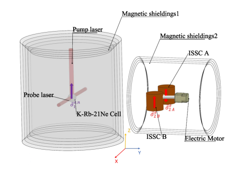
Figure 2: (Color online)The experimental setup. The left side was the SERF co-magnetometer. The two ISSC spin sources noted as 2A and 2B were driven by a servo motor, and they could rotate CW and CCW along y axis with a given frequency.

Driven by a servo motor, the ISSCs rotated with a frequency of $f_{0}=5.25$ Hz clockwise (CW) or counter-clockwise (CCW). Because the two ISSCs were mounted centrosymmetrically, the frequency of the possible SSVDF signals detected by the SERF was doubled, i.e. 10.5 Hz. This frequency was chosen due to the facts that the SERF co-magnetometer had relatively large responses to both $B^{e}_{eff,x}$ and $B^{e}_{eff,y}$ (Fig. 1), as well as relatively low noise level here (Fig. 3). When rotating to a given angle, the ISSCs could trigger an optoelectronic pulse, and this signal was recorded by the data-acquisition system. This signal was used as the starting point of a new cycle for data analysis. Similar to the SERF, the ISSCs as well as the servo motor were both shielded by 4 layers of $\mu$-metal to further reduce possible magnetic field leakage from the ISSCs and servo motor.

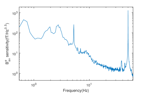
Figure 3: A typical power spectrum measured in the experiment. The ISSCs rotated in the frequency of 5.25 Hz, and the motor power system may cause the peak at 5.25 Hz in the spectrum. The 50 Hz peak in the spectrum came from the power supply of the equipment, which was 50 Hz, 220V.

Data Analysis–

The experimental raw data was recorded as $\mathbf{S}^{exp}_{i,raw}(t_{j})$, where $i$ and $j$ mean the $j$-th point in the $i$-th cycle, $t_{j}=j*\Delta t$, and $\Delta t$ is the data sampling period. Then, $\mathbf{S}^{exp}_{i,raw}(t_{j})$ was first transformed to frequency domain by using Fast Fourier Transformations (FFT). A typical SERF power spectrum is shown in Fig.3. Then Gaussian filters were applied to remove the peaks corresponding to 5.25 and 50 Hz. After that, the signals were transformed back to the time domain with inverse FFT. Furthermore, DC components in $\mathbf{S}^{exp}_{i,raw}(t_{j})$ were also removed. After the steps above, the raw signals $\mathbf{S}^{exp}_{i,raw}(t_{j})$ were then transferred to $\mathbf{S}^{exp}_{i}(t_{j})$ for further analysis.

Expected signals $S^{sim}(t)$ sensed by the SERF could be simulated by solving the equation sets (2) and (3) with the experimental parameters and a tentative coupling constant $f_{16}^{(tn)}$ in $V_{16}$ as inputs. In the parameter space that we were interested in, i.e., $B_{eff}<1$ nT, $P_{x}^{e}(t)$ approximately linearly dependent on $B_{eff}$, and thereafter the coupling constant $f_{16}$. The $S^{sim}(t)$ then linearly depended on $B_{eff}$, i.e. $S^{sim}(t)\simeq\kappa f_{16}^{(tn)}\,B_{eff}$, where $\kappa$ is the calibration constant, which was measured to be $110\pm 5$ V/nT. The input $B_{eff}$ for solving Eq. 2&3 were simulated by the finite element analysis methodJi et al. (2017). Two examples of simulated signals for $V_{16}$, the $\mathbf{S}^{sim}_{16}$, with motor rotating CW and CCW are shown in Fig. 4(a).

The experimental signals $\mathbf{S}^{exp}_{i}(t_{j})$ were then compared with the simulated ones $S^{sim}(t)$. A cosine similarity score $k_{i}$ was used to weigh the similarity between $\mathbf{S}^{exp}_{i}$ and a given reference signal $\mathbf{S}^{ref}(t)$, which can be written as Krasichkov et al. (2015),

$$k_{i}\equiv\frac{\sum_{j}\mathbf{S}^{ref}(t_{j})\cdot{\mathbf{S}}_{i}^{exp}(t_{j})}{\sqrt{\sum_{j}\left[\mathbf{S}^{ref}(t_{j})\right]^{2}}\sqrt{\sum_{j}\left[{\mathbf{S}_{i}}^{exp}(t_{j})\right]^{2}}}.$$ (4)

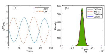
Figure 4: (Color online) (a) The simulated $\mathbf{S}^{sim}_{16}$ signals with $f^{(tn)}_{16}=1\times 10^{-4}$, $\lambda=1000$ when motor rotates CW (blue solid line) and CCW (red dashed line). (b) The distribution of the $f_{i}^{exp}$ with $S^{ref}=S^{sim}_{16}$. The black area represents the ISSCs rotating CW, and green area CCW. The red dashed line and blue solid line are their Gaussian fit respectively.

The coupling constant in $V_{16}$ measured experimentally in $i$-th cycle, $f^{exp}_{i,16}$, can be written as,

$$f^{exp}_{i,16}=k_{i}f_{16}^{(tn)}\,\sqrt{\frac{\sum_{j}\left[\mathbf{S}^{exp}_{i}(t_{j})\right]^{2}}{\sum_{j}\left[\mathbf{S}^{ref}(t_{j})\right]^{2}}}.$$ (5)

Distributions of $f^{exp}_{i,16}$ are shown in Fig. 4(b). They agree with Gaussian shapes well.

The final experimentally measured coupling constant $f^{exp}_{16}$ was obtained by averaging all rotating cycles including CW and CCW, i.e.

$$f^{exp}_{16}=\frac{\langle f^{exp}_{i,16}\rangle_{+}+\langle f^{exp}_{i,16}\rangle_{-}}{2},$$ (6)

where $\langle f^{exp}_{i,16}\rangle_{+}=\frac{1}{n}\sum_{i=1}^{n}f^{exp}_{i,16}$ is the average over the CW cycles, and $\langle f^{exp}_{i,16}\rangle_{-}$, the CCW cycles.

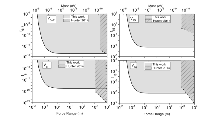
Figure 5: Limits on the SSVDFs’ coupling constants between two electrons measured in this work, and comparison with those in literature. The ”Hunter2014” comes from Ref. Hunter and Ang (2014), in which polarized geo-electrons were used.

Results and Discussion–

The other terms of SSVDFs Dobrescu and Mocioiu (2006); Leslie et al. (2014) were analyzed by the same method. These interactions were:

$$V_{\rm 6+7}= \frac{-f_{6+7}\hbar^{2}}{4\pi m_{\mu}c}(\hat{\bm{\sigma}_{1}}\cdot\mathbf{v})(\hat{\bm{\sigma}}_{2}\cdot\hat{\bm{r}})\left(\ \frac{1}{\lambda r}+\frac{1}{r^{2}}\right)e^{-r/\lambda},$$ (7)

$$\begin{split}V_{8}&=\frac{f_{8}\hbar}{4\pi c}(\hat{\bm{\sigma}_{1}}\cdot\mathbf{v})(\hat{\bm{\sigma}_{2}}\cdot\mathbf{v})\frac{e^{-r/\lambda}}{r}\end{split},$$ (8)

$$\begin{split}V_{15}=&\frac{-f_{15}\hbar^{3}}{8\pi m_{1}m_{2}c^{2}}\big{\{}(\hat{\bm{\sigma}_{2}}\cdot\hat{\bm{r}})\left[\hat{\bm{\sigma}_{1}}\cdot(\mathbf{v}\times\hat{\bm{r}})\right]+(\hat{\bm{\sigma}_{1}}\cdot\hat{\bm{r}})\\ &\left[\hat{\bm{\sigma}_{2}}\cdot(\mathbf{v}\times\hat{\bm{r}})\right]\big{\}}\left(\frac{1}{\lambda^{2}r}+\frac{3}{\lambda r^{2}}+\frac{3}{r^{3}}\right)e^{-r/\lambda}.\end{split}$$ (9)

The parameters of the setup and their errors are shown in Tab. 1. Considering these errors, together with the statistical error, the constraints on the SSVDFs between two electrons could be set. The results are shown in Fig. 5. The gray areas are excluded with 95% confidence level. For $V_{6+7}$, $V_{8}$, $V_{15}$, and $V_{16}$, our experiment can set up new record limits at the range of 5 cm – 1 km. Especially for $V_{15}$, our result is over 3 orders of magnitude better than (Hunter and Ang, 2014) in force range between 5 cm and 1 km.

The error budget for $f^{exp}_{i,16}$ at $\lambda=1.1$ m is shown in Tab. 1. The major systematic error came from the cross-talking between the servo motor power system and the SERF system. The 5.25 Hz peak shown in Fig. 3 might come from cross-talking effect. However, the major frequency considered here was 10.5 Hz, whose amplitude was about 40 times smaller than 5.25 Hz. The secondary harmonics of 5.25 Hz could also contribute to systematic error. In fact, the correlation between 5.25 Hz and 10.5 Hz could be calculated by applying $\mathbf{S}^{ref}_{A}(t_{j})=\sin[5.25t_{j}]$ or $\mathbf{S}^{ref}_{B}(t_{j})=\sin[10.5t_{j}]$ to Eq.(4). A correlation between 5.25 and 10.5 Hz was indeed found this way, which confirmed the cross-talking effect. The cross-talking was the dominant effect in our experiment.

Another major consideration was the magnetic leakage from the ISSCs. With the iron shielding, at a distance of 20 cm away from the ISSC’s mass center, its residual magnetic field was measured to be $<10$ mG. The magnetic shielding factors for the mu-metals outside the ISSCs were measured to be $>10^{6}$, and shielding for SERF magnetometer, $>2\times 10^{6}$. Considering all factors together, we conservatively expect the magnetic leakage from the ISSCs to SERF’s center to be smaller than $10^{-2}$ aT, which was insignificant in regards to the error budget.

It is worth pointing out that only the errors of the parameters when doing the calculation of $f^{sim}$ as well as the statistic uncertainty could affect the limit curves drawn in Fig. 5. The magnetic field leakage and cross-talking were not subtracted in these plots.

Table 1: Input parameters for the FEA simulation and their error contribution to the final uncertainties. The origin of coordinates was at the center of the pumping cell.

Parameter	Value	$\Delta f^{exp}_{16}(\times 10^{-8})$
ISSC net spin ($\times 10^{24}$)	$1.75\pm 0.21$	${}^{+0.34}_{-0.32}$
Position of ISSCs y(m)	$-0.624\pm 0.005$	${}^{+0.13}_{-0.12}$
Position of ISSCs z(m)	$0.278\pm 0.005$	$\pm 0.04$
D between 2 ISSCs(m)	$0.251\pm 0.001$	$\pm 0.03$
Rotating frequency(Hz)	$5.250\pm 0.001$	$<0.001$
Calib. const. $\kappa$ (V/nT)	$330\pm 20$	$\pm 0.23$
phase uncertainty ($\deg$)	$\pm 5$	$\pm 0.27$
Final $f^{exp}_{16}(\times 10^{-8})$	$4.0$	$\pm 1.9\ (statistic)$
$(\lambda=1.1m)$		$\pm 0.5$

Summary–

In summary, by using specially designed iron-shielded SmCo₅ permanent magnets, a high electron spin density source of about $1.7\times 10^{21}$ cm^-3 has been achieved, while still keeping its magnetic leakage down to about mG level. The similarity analysis have been proved to be successful, which gives a boost to the detecting sensitivities. With help from the high spin density, the high sensitive SERF co-magnetometer, and the similarity analysis, new constraints on possible new exotic potentials of $V_{6+7}$, $V_{8}$, $V_{15}$, and $V_{16}$ were derived for force range of 5 cm – 1 km. To the best of our knowledge, it is the first time these results have beem attained. By dedication to improving the SERF sensitivities, and reducing the crossing-talking effect, a higher sensitivity by a factor of over 1000 is expected in future studies with a similar experimental setup.