Optimal Threshold-Based Control Policies for Persistent Monitoring on Graphs

Abstract

We consider the optimal multi-agent persistent monitoring problem defined by a team of cooperating agents visiting a set of nodes (targets) on a graph with the objective of minimizing a measure of overall node state uncertainty. The solution to this problem involves agent trajectories defined both by the sequence of nodes to be visited by each agent and the amount of time spent at each node. Since such optimal trajectories are generally intractable, we propose a class of distributed threshold-based parametric controllers through which agent transitions from one node to the next are controlled by threshold parameters on the node uncertainty states. The resulting behavior of the agent-target system can be described by a hybrid dynamic system. This enables the use of Infinitesimal Perturbation Analysis (IPA) to determine on line (locally) optimal threshold parameters through gradient descent methods and thus obtain optimal controllers within this family of threshold-based policies. We further show that in a single-agent case the IPA gradient is monotonic, which implies a simple structure whereby an agent visiting a node should reduce the uncertainty state to zero before moving to the next node. Simulation examples are included to illustrate our results and compare them to optimal solutions derived through dynamic programming when this is possible.

I Introduction

The cooperative multi-agent persistent monitoring problem arises when agents are tasked to monitor a dynamically changing environment which cannot be fully covered by a stationary agent allocation. Thus, persistent monitoring differs from traditional consensus [1] and coverage control [2] problems due to the continuous need to explore changes in the environment. In many cases, this exploration process leads to the discovery of various “points of interest”, which, once detected, become “data sources” or “targets” that need to be perpetually monitored. This paradigm applies to surveillance systems, such as when a team must monitor large regions for changes, intrusions, or other dynamic events [3], or when it is responsible for sampling and monitoring environmental parameters such as temperature [4]. It also finds use in particle tracking in molecular biology where the goal is to track multiple individual biological macromolecules to understand their dynamics and their interactions [5, 6]. In contrast to sweep coverage and patrolling [7, 8], the problem we address here focuses on a finite number of data sources or “targets” (typically larger than the number of agents). The goal of the agent team is to collect information from each target so as to reduce a metric of uncertainty about its state. This uncertainty naturally increases while no agent is present in its vicinity and decreases when it is being monitored (or “sensed”) by one or more agents. Thus, the objective is to minimize an overall measure of target uncertainty by controlling the movement of all agents.

Our previous work [9] considered the persistent monitoring problem in a one-dimensional space, formulated it as an optimal control problem and showed that the solution can be reduced to a parametric controller form. In particular, the optimal agent trajectories are characterized by a finite number of points where each agent switches direction and by a dwell time at each such point. However, in two-dimensional (2D) spaces, it has been shown that such parametric representations for optimal agent trajectories no longer hold [8]. Nonetheless, various forms of parametric trajectories (e.g., ellipses, Lissajous curves, interconnected linear segments) can still be near-optimal or at least offer an alternative [8, 10]. These approaches limit agent trajectories to certain forms which, while they possess desirable properties (e.g., periodicity), cannot always capture the dynamic changes in target uncertainties and may lead to poor local optima [11, 12, 9].

In this paper, we take a different direction in the 2D persistent monitoring problem. Rather than parameterizing agent trajectories, we adopt a more abstract point of view whereby targets are nodes in a graph and their connectivity defines feasible agent trajectories along the edges of the graph. A trajectory is specified by a sequence of nodes and an associated dwell time at each node in the sequence. In this setting, there is a travel time defined for each edge in the graph which is determined in advance according to the actual target topology and has the added benefit of accounting for constraints such as physical obstacles in the 2D space which the graph is designed to avoid. The controller associated with each agent determines $(i)$ the dwell time at the current node and $(ii)$ the next node to be visited with the goal of optimizing a given performance metric. The complexity in this optimization problem is significant [13] and the presence of real-valued dwell time decision variables makes it much harder than that of Traveling Salesman Problems [14], which are already computationally intensive and do not scale well. Since deriving such optimal trajectories is generally intractable, we consider a class of controllers based on a set of threshold parameters associated with the target uncertainties, hence taking into account the time-varying nature of target states. Thus, the parameterization in this graph-based setting is imposed on the target thresholds rather than on the shape of agent trajectories in the underlying 2D Euclidean environment. By adjusting the thresholds, we can control the agent behavior in terms of target visiting and dwelling and, therefore, optimize a given performance metric within the specific parametric controller family considered. From a modeling standpoint, this results in a hybrid dynamic system whose state consists of agent positions and target uncertainties. From an optimization standpoint, the goal is to determine optimal thresholds (parameters) that minimize a given metric.

The contribution of the paper lies in the graph-based setup of the 2D persistent monitoring problem, the formulation of a threshold-based parametric optimization problem, and a solution approach based on Infinitesimal Perturbation Analysis (IPA) [15] to determine on line the gradient of the objective function and to obtain (possibly local) optimal threshold parameters through gradient descent. As we will see, optimizing these thresholds not only affects the dwell time that the agent should spend at each node, but also naturally adjusts and seeks to optimize the node visiting sequence. Our approach is distributed since the decisions made by an agent at some node are based on uncertainty states of neighboring nodes only. Moreover, we exploit the event-driven nature of IPA to also render it scalable in the number of events in the system and not the state space (in contrast to solutions dependent on dynamic programming). An additional contribution is to show that in the case of a one-agent system the IPA gradient is monotonic in the thresholds involved which implies a simple optimal structure: the agent visiting a node should reduce the uncertainty state to zero before moving to the next node. This is consistent with a similar earlier result established in [13].

The paper is organized as follows. Section II formulates the 2D persistent monitoring problem on a graph and introduces the parametric family of threshold-based agent controllers we subsequently analyze. Section III provides a solution of the optimization problem obtained through event-driven IPA gradient estimation. In Section IV, we present our analysis of the one-agent case with the key result that all optimal dwell times are specified by zero threshold values. Section V includes simulation examples, including comparisons with optimal solutions derived through dynamic programming when this is possible. Section VI concludes the paper.

II Problem formulation

Consider $N$ agents and $M$ targets in a 2D mission space. The agent positions are $s_{a}(t)\in\mathbb{R}^{2}$, $a=1,\dots,N$ and the target locations are $X_{i}\in\mathbb{R}^{2}$, $i=1,\dots,M$.

Target uncertainty model. Following the model in [9], we define uncertainty functions $R_{i}(t)$ associated with targets $i=1,\ldots,M$, with the following properties: $(i)$ $R_{i}(t)$ increases with a prespecified rate $A_{i}$ if no agent is visiting it, $(ii)$ $R_{i}(t)$ decreases with a rate $B_{i}N_{i}(t)$ where $B_{i}$ is the rate at which an agent collects data from target $i$, hence decreasing its uncertainty state, and $N_{i}(t)=\sum_{a=1}^{N}\mathbf{1}\{s_{a}(t)=X_{i}\}$ is the number of agents at target $i$ at time $t$, and $(iii)$ $R_{i}(t)\geq 0$ for all $t$. We model the target uncertainty state dynamics as follows:

$$\dot{R}_{i}(t)=\left\{\begin{array}[c]{ll}0&\text{if }R_{i}(t)=0\text{ and }A_{i}\leq B_{i}N_{i}(t)\\ A_{i}-B_{i}N_{i}(t)&\text{otherwise }\end{array}\right.$$ (1)

This model has an attractive queueing system interpretation as explained in [9], where each target is associated with an “uncertainty queue” with input rate $A_{i}$ and service rate $B_{i}N_{i}(t)$ controllable through the agent movement. Note that compared with the model in [9], where each agent has a finite sensing range $r_{a}$ allowing it to decrease $R_{i}(t)$ as long as $\left\|s_{a}(t)-X_{i}\right\|<r_{a}$, here the agent’s sensing range is ignored and the joint detection probability of a target by agents is replaced by the summation $N_{i}(t)$ above. This is done for simplicity to accommodate the graph topology we will adopt; the analysis can be extended to the original model in [9] at the expense of added notation and the use of a sensing model for each agent.

Agent model. The position of agent $a$ is denoted by $s_{a}(t)=[x_{a}(t),y_{a}(t)]^{\top}$ for $a=1,\ldots,N$ and its dynamics in 2D are given by:

$$\dot{s}_{a}(t)=[v_{a}(t)\cos(u_{a}(t)),v_{a}(t)\sin(u_{a}(t))]^{\top}$$ (2)

where the agent’s velocity is scaled and bounded such that $\|v_{a}(t)\|\leq 1$ and the agent’s heading is $u_{a}(t)\in[0,2\pi)$.

Objective function. Our goal is to determine the optimal control (both $v_{a}(t)$ and $u_{a}(t)$) for all agents under which the average uncertainty metric in (3) across all targets is minimized over a given time horizon $T$. Setting $\mathbf{v}(t)=[v_{1}(t),\ldots,v_{N}(t)]$ and $\mathbf{u}(t)=[u_{1}(t),\ldots,u_{N}(t)]$, we aim to solve the following optimal control problem:

$$\mathbf{P1:}\min_{\mathbf{v}(t),\mathbf{u}(t)}\text{ \ }J=\frac{1}{T}\int_{0}^{T}\sum_{i=1}^{M}R_{i}(t)\,dt$$ (3)

subject to target dynamics in (1) and agent dynamics in (2).

Obtaining a complete solution of P1 generally requires solving a computationally hard Two Point Boundary Value Problem (TPBVP) which amounts to a 2D functional search in both $v_{a}(t)$ and $u_{a}(t)$ for each agent over $t\in[0,T]$. Unlike the 1D case in [9], the problem cannot be reduced to a parametric one as shown in [8]. However, it is still easy to show that the optimal agent speed is limited to $\|v_{a}^{\star}(t)\|\in\{1,0\}$ depending on whether the agent is dwelling or traveling. In particular, the Hamiltonian associated with P1 is

$$\begin{split}H=&\sum_{i=1}^{M}R_{i}(t)+\sum_{i=1}^{M}\lambda_{i}(t)\dot{R}_{i}(t)\\ &+\sum_{a=1}^{N}v_{a}\left(\lambda_{a}^{x}(t)\cos u_{a}(t)+\lambda_{a}^{y}(t)\sin u_{a}(t)\right)\end{split}$$ (4)

and a straightforward application of the Pontryagin minimum principle implies that $v_{a}^{\ast}(t)=\pm 1$ depending on the sign of $\left(\lambda_{a}^{x}(t)\cos u_{a}(t)+\lambda_{a}^{y}(t)\sin u_{a}(t)\right)$, or $v_{a}^{\ast}(t)=0$ in singular arcs that may exist. The analysis is similar to the one in [8] and is, therefore, omitted here.

Using this optimal control structure and the underlying target topology, we make a further simplification by constraining agent movements to a graph $G=(V,E)$ where the set of vertices (nodes) is defined by an indexed list of targets $V=\{1,\ldots,M\}$ and the set of edges (links) $E$ contains all feasible direct connections between them. Note that if there are obstacles in the underlying space, we can introduce “way points” to define feasible paths avoiding the obstacles, where a way point $j$ is included in the set $V$ with an associated uncertainty state $R_{j}(t)=0$ for all $t\geq 0$. In this graph topology, the agent headings $u_{a}(t)$ are limited to the finite set $V$, i.e., $u_{a}(t)\in V=\{1,\ldots,M\}$.

Therefore, we have reduced P1 to a simpler problem of determining $(i)$ the dwell time for each agent at each node when $v_{a}(t)=0$ and $(ii)$ the control (heading) $u_{a}(t)$ when $v_{a}(t)\neq 0$. The complete state of this system is defined by $\mathbf{s}(t)=[s_{1}(t),\ldots,s_{N}(t)]$ and $\mathbf{R}(t)=[R_{1}(t),\ldots,R_{M}(t)]$ so that the control should be expressed as $u_{a}(\mathbf{s}(t),\mathbf{R}(t))$.

Figure 1 shows a typical control trajectory and helps pinpoint the behavior of each agent controller. The trajectory consists of a sequence of intervals $[t_{a,k},t_{a,k+1})$ where the agent’s node visits are indexed by $k=1,2,\ldots$ and $t_{a,k}$ is the time of the $k$-th visit at any node. This interval contains $t_{a,k}+d_{a,k}$, the time when the agent leaves the current node it is visiting. Note that on an optimal trajectory:

$$t_{a,k+1}^{\ast}=t_{a,k}^{\ast}+d_{a,k}^{\ast}+\|s_{a}^{\ast}(t_{a,k})-s_{a}^{\ast}(t_{a,k+1})\|$$

since the optimal agent speed when transitioning between nodes satisfies $\|v_{a}^{\star}(t)\|=1$. Thus, the agent controller’s role when visiting some node $i$ is to determine the optimal dwelling time $d_{a,k}^{\ast}$ and next node $u_{a}^{\ast}(t_{a,k}^{\ast}+d_{a,k}^{\ast})$. Clearly, $u_{a}(t)$ is a piecewise constant right-continuous function of time and the values of $u_{a}(t)$ belong to the set

$$u_{a}\left(t\right)\in\{i\}\cup\mathcal{N}_{i}\quad\text{ if }s_{a}(t)=X_{i}$$ (5)

where $\mathcal{N}_{i}$ is the neighborhood of node $i$ defined as follows.

Figure 1: An agent control trajectory: $d_{a,k}$ is the $k$-th dwell time and $tr_{a,k}$ is the $k$-th travel time.

Definition 1.

The neighborhood of node $i$ is the set $\mathcal{N}_{i}=\{j:(i,j)\in E,$ $j\in V\}$.

Since the control $u_{a}\left(t\right)$ switches only at times $t_{a,k}+d_{a,k}$ (see Fig. 1), let us concentrate on a time interval $[t_{a,k},t_{a,k}+d_{a,k})$ during which $s_{a}(t)=X_{i}$ for some $i\in V$. Observe that for $t\geq t_{a,k}$ either $u_{a}\left(t\right)=i$ or it switches to a new value $j\in\mathcal{N}_{i}$. The condition under which such a switch occurs may generally be expressed as $g_{i,j}(\mathbf{s}(t),\mathbf{R}(t))\leq 0$, i.e., $g_{i,j}(\mathbf{s}(t),\mathbf{R}(t))$ is a switching function associated with a transition from node $i$ to node $j$. Let us define

$$\tau_{a,k}^{j}=\inf_{t\geq t_{a,k}}\{g_{i,j}(\mathbf{s}(t),\mathbf{R}(t))=0\}$$

and set

$$t_{a,k}+d_{a,k}=\min_{j\in\mathcal{N}_{i}}\{\tau_{a,k}^{j}\}$$

so that the change in the agent’s node assignment occurs at the earliest time that one of the switching functions satisfies $g_{i,j}(\mathbf{s}(t),\mathbf{R}(t))=0$. Thus, the task of the controller is to determine optimal switching functions $g_{i,j}^{\ast}(\mathbf{s}(t),\mathbf{R}(t))$ for all $j\in\mathcal{N}_{i}$ whenever $s_{a}(t)=X_{i}$ and then evaluate $\min_{j\in\mathcal{N}_{i}}\{\tau_{a,k}^{j}\}$ to specify the optimal dwelling time $d_{a,k}^{\ast}$. Therefore,

$$u_{a}^{\ast}\left(t\right) =i\text{, \, }t\in[t_{a,k}^{\ast},t_{a,k}^{\ast}+d_{a,k}^{\ast})$$ (6)

$$u_{a}^{\ast}\left(t_{a,k}^{\ast}+d_{a,k}^{\ast}\right) =\arg\min_{j\in\mathcal{N}_{i}}\{\tau_{a,k}^{j}\}$$

In effect, whenever $s_{a}(t)=X_{i}$, the state space defined by all feasible values of $[\mathbf{s}(t),\mathbf{R}(t)]$ is partitioned into $\left|\mathcal{N}_{i}\right|+1$ regions, denoted by $\mathcal{R}_{i}$ and $\mathcal{R}_{j}$, $j\in\mathcal{N}_{i}$. The controller keeps the agent at node $i$ as long as $[\mathbf{s}(t),\mathbf{R}(t)]\in\mathcal{R}_{i}$ and switches to $u_{a}\left(t\right)=j\in\mathcal{N}_{i}$ as soon as the state vector transitions to a new region $\mathcal{R}_{j}$. Thus, the optimization problem consists of determining an optimal partition for all $i=1,\ldots,M$ through $g_{i,j}^{\ast}(\mathbf{s}(t),\mathbf{R}(t))$ for all $j\in\mathcal{N}_{i}$ and the time of  a transition from $\mathcal{R}_{i}$ to some $\mathcal{R}_{j}$, $j\in\mathcal{N}_{i}$.

Finally, given control $u_{a}(t)$, the agent’s physical dynamics over $t\in[t_{a,k},t_{a,k+1})$ are given by

$$\dot{s}_{a}(t)=\left\{\begin{array}[c]{cl}\frac{X_{i}-s_{a}(t)}{\|X_{i}-s_{a}(t)\|}&\text{if }t\in[t_{a,k}+d_{a,k},t_{a,k+1})\\ 0&\text{otherwise}\end{array}\right.$$ (7)

for some $i=u_{a}(t)\in V$.

Parametric control. As already mentioned, designing an optimal feedback controller for P1 in a 2D space is generally intractable. The problem remains hard even in the simplified graph topology embedded in the original 2D space where optimal partitions of the state space must be determined whenever an agent visits a node. Therefore, an alternative is to seek a parameterization of these partitions through a parameter vector $\mathbf{\Theta}$ so as to ultimately replace P1 by a problem requiring the determination of an optimal parameter vector $\mathbf{\Theta}^{\ast}=\arg\min J(\mathbf{\Theta})$ over the set of feasible values of $\mathbf{\Theta}$. Thus, switching functions of the form $g_{i,j}(\mathbf{s}(t),\mathbf{R}(t))$ are expressed as $g_{i,j}(\mathbf{s}(t),\mathbf{R}(t);\mathbf{\Theta})$ and an optimal switching function is given by $g_{i,j}(\mathbf{s}(t),\mathbf{R}(t);\mathbf{\Theta}^{\ast})$.

The parameterization we select in our problem is motivated by the observation that the movement of agents should be determined based on the values of the target uncertainty states available to an agent, since the cost function (3) is closely related to these values. Thus, we introduce threshold parameters associated with a node $i$ which, when compared to the actual value of $R_{i}(t)$, provide information about the importance of visiting this node next when an agent is in its neighborhood and needs to evaluate the control in (6). We set the thresholds to be distinct when the agent is at different nodes, thus rendering the control policy more flexible since it depends on both node uncertainty values and the agent’s position.

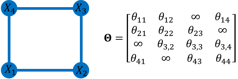
We represent the node thresholds associated with agent $a$ by an $M\times M$ matrix $\bm{\Theta}^{a}$ where each row represents the index of the current node visited by $a$ and a column represents the index of a potential next node to visit. An example is shown in Fig. 2 where a threshold parameter is set to $\infty$ when there is no direct path between the corresponding nodes. In this example, an agent located at node $1$ uses a state space partition parametrized by $\theta_{11}$, $\theta_{12}$ and $\theta_{14}$. The overall parameter matrix accounting for all agents is denoted by $\bm{\Theta}$ of dimension $M\times M\times N$.

Figure 2: A 1-agent 4-target example. The target topology graph is shown on the left and the threshold matrix is on the right.

Next, we define the specific threshold-based controller family we consider. The starting point is to define a state space region forcing the agent to remain at node $i$. This is expressed through the condition $R_{i}(t)>\theta_{ii}^{a}$. When this is no longer met, i.e., the uncertainty state at node $i$ is sufficiently low with respect to a level $\theta_{ii}^{a}$, then the agent may be assigned to a new node $j\neq i$ as long as its uncertainty state exceeds another threshold, i.e., $R_{j}(t)\geq\theta_{ij}^{a}$. Since there may be several nodes in the neighborhood of $i$ whose uncertainty states are high relative to their associated thresholds, we prioritize nodes in the neighborhood of $i$ by defining an ordered set for agent $a$ as follows:

$$\mathcal{N}_{i}^{a}=\{j_{k}\in\mathcal{N}_{i}:j_{1},\ldots,j_{k},\ldots,j_{D_{i}}\}$$

where $D_{i}$ is the degree of vertex $i$ (the number of edges connected to vertex $i$). Although the prioritization scheme used may depend on several factors, in what follows we assume that $\|X_{j_{k}}-X_{i}\|<\|X_{j_{k+1}}-X_{i}\|$ for all $k=1,\ldots,D_{i}$, i.e., the neighbors are ordered based on their relative proximity to node $i$.

We now define the threshold-based control to specify $u_{a}(t;\bm{\Theta})$ in (6) as follows:

$$u_{a}(t;\bm{\Theta})=\left\{\begin{split}&i\qquad\qquad\qquad\qquad\qquad\text{ if }R_{i}(t)>\theta_{ii}^{a}\text{ or }\\ &\qquad\qquad\qquad\qquad R_{j}(t)<\theta_{ij}^{a}\text{ for all }j\in\mathcal{N}_{i}^{a}\\ \\ &\arg\min_{\begin{subarray}{c}k\\ \text{s.t.}j_{k}\in\mathcal{N}_{i}^{a}\end{subarray}}R_{j_{k}}\geq\theta_{ij_{k}}^{a}\qquad\text{ otherwise}\end{split}\right.$$ (8)

Under (8), the agent first decreases $R_{i}(t)$ below the threshold $\theta_{ii}^{a}$ before moving to another node in the neighbor set $\mathcal{N}_{i}^{a}$ with the minimum index $k$ whose associated state uncertainty value exceeds the threshold $\theta_{ij_{k}}^{a}$. If no such neighbor exists, the agent remains at the current node maintaining its uncertainty state under the given threshold level. All agent behaviors are therefore entirely governed by $\bm{\Theta}$ through (8), which also implicitly determines the dwell time of the agent at node $i$.

Remark 1.

The controller in (8) is designed to be distributed by considering only the states of neighboring nodes and not those of other nodes or of other agents. As such, it is limited to a one-step look-ahead policy. However, it can be extended to a richer family of more general multi-step look-ahead policies based on node uncertainty state thresholds. While this causes the dimensionality of $\bm{\Theta}$ to increase, the optimization framework presented in Sec. III is not affected.

Under (8), P1 is reduced to a simpler parametric optimization problem of determining the optimal thresholds in matrix $\bm{\Theta}^{\star}$ under which the cost function in (3) is minimized. Moreover, the resulting agent and node behavior defines a hybrid system: the node dynamics in (1) switch between the mode where $\dot{R}_{i}(t)=0$ and $\dot{R}_{i}(t)=A_{i}-B_{i}N_{i}(t)$ with $N_{i}(t)=0,1,\ldots,N$, while the agent dynamics in (7) experience a switch whenever there is a sign change in some expression of the form $(R_{j}(t)-\theta_{ij}^{a})$ as seen in (8), hence triggering a control switch. We rewrite the cost in (3) as the sum of costs over all intervals $\left[\tau_{k},\tau_{k+1}\right)$ for $k=0,\ldots,K$ where $\tau_{k}$ is the time instant when any of the state variables experiences a mode switch (these will be explicitly defined as “events” in the sequel) and $\tau_{K}=T$ denotes the end of the time horizon as shown in (9). Therefore, we have transformed the optimal control problem P1 into a simpler parametric optimization problem P2 as follows:

$$\mathbf{P2:}\min_{\bm{\Theta}\geq\mathbf{0}}\text{ \ }J(\bm{\Theta})=\frac{1}{T}\sum_{i=1}^{M}\sum_{k=0}^{K}\int_{\tau_{k}}^{\tau_{k+1}}R_{i}(t)\,dt$$ (9)

subject to target uncertainty dynamics (1), agent state dynamics (7) and the control policy (8).

Remark 2.

Using the optimal threshold matrix $\bm{\Theta}^{\star}$, the optimal dwell times and target visiting sequences can both be determined on line while executing the control policy (8). It is interesting to note that, despite the a priori prioritization imposed in $\mathcal{N}_{i}^{a}$, the actual target visiting sequence will be adjusted as a result of the thresholds being adjusted during the optimization process. This is because the optimization process will decrease the threshold values of nodes that maintain higher uncertainties, hence inducing agents to visit them more frequently.

III Infinitesimal Perturbation Analysis (IPA)

In the previous section, agent trajectories are selected from the family $\mathbf{s}(\bm{\Theta},\mathbf{s}_{0},\mathbf{R}_{0})$ with parameter $\bm{\Theta}$ and given initial agent positions $\mathbf{s}_{0}$ and node uncertainty states $\mathbf{R}_{0}$. The state dynamics are governed by (1) and (7) under the control policy (8). An “event” is defined as any discontinuous change in any one of the state variables (e.g., a threshold has been met by some $R_{i}(t)$). The $k$-th event occurrence time is denoted by $\tau_{k}(\bm{\Theta})$. We use Infinitesimal Perturbation Analysis (IPA) to obtain on line the gradient of the cost function in (9) with respect to the parameters in $\bm{\Theta}$, hence seeking an optimal solution through a gradient descent process. IPA specifies how changes in the parameter $\bm{\Theta}$ influence event times $\tau_{k}(\bm{\Theta})$, $k=1,2,\ldots$, the trajectories $\mathbf{s}(\bm{\Theta},\mathbf{s}_{0},\mathbf{R}_{0})$, and ultimately the cost function (9). We first briefly review the IPA framework for general hybrid systems as presented in [15] and then apply it to our specific setting.

Let $\{\tau_{k}(\theta)\}$, $k=1,\ldots,K$, denote the occurrence times of all events in the state trajectory of a hybrid system with dynamics $\dot{x}\ =\ f_{k}(x,\theta,t)$ over an interval $[\tau_{k}(\theta),\tau_{k+1}(\theta))$, where $\theta\in\Theta$ is some parameter vector and $\Theta$ is a given compact, convex set. For convenience, we set $\tau_{0}=0$ and $\tau_{K+1}=T$. We use the Jacobian matrix notation: $x^{\prime}(t)\equiv\frac{\partial x(\theta,t)}{\partial\theta}$ and $\tau_{k}^{\prime}\equiv\frac{\partial\tau_{k}(\theta)}{\partial\theta}$, for all state and event time derivatives. It is shown in [15] that

$$\frac{d}{dt}x^{\prime}(t)=\frac{\partial f_{k}(t)}{\partial x}x^{\prime}(t)+\frac{\partial f_{k}(t)}{\partial\theta},$$ (10)

for $t\in[\tau_{k},\tau_{k+1})$ with boundary condition:

$$x^{\prime}(\tau_{k}^{+})=x^{\prime}(\tau_{k}^{-})+[f_{k-1}(\tau_{k}^{-})-f_{k}(\tau_{k}^{+})]\tau_{k}^{\prime}$$ (11)

for $k=1,...,K$. In order to complete the evaluation of $x^{\prime}(\tau_{k}^{+})$ in (11), we need to determine $\tau_{k}^{\prime}$. If the event at $\tau_{k}$ is exogenous (i.e., independent of $\theta$), $\tau_{k}^{\prime}=0$. However, if the event is endogenous, there exists a continuously differentiable guard function $g_{k}:\mathbb{R}^{n}\times\Theta\rightarrow\mathbb{R}$ such that $\tau_{k}\ =\ \min\{t>\tau_{k-1}\ :\ g_{k}\left(x\left(\theta,t\right),\theta\right)=0\}$ and

$$\tau_{k}^{\prime}=-[\frac{\partial g_{k}}{\partial x}f_{k}(\tau_{k}^{-})]^{-1}(\frac{\partial g_{k}}{\partial\theta}+\frac{\partial g_{k}}{\partial x}x^{\prime}(\tau_{k}^{-}))$$ (12)

as long as $\frac{\partial g_{k}}{\partial x}f_{k}(\tau_{k}^{-})\neq 0$ (details can be found in [15]).

Differentiating the cost $J(\bm{\Theta})$ in P2, we obtain

$$\nabla J(\bm{\Theta})= \frac{1}{T}\sum_{i=1}^{M}\sum_{k=0}^{K}\Bigg{(}\int_{\tau_{k}}^{\tau_{k+1}}\nabla R_{i}(t)\,dt$$

$$+R_{i}(\tau_{k+1})\nabla\tau_{k+1}-R_{i}(\tau_{k})\nabla\tau_{k}\Bigg{)}$$

$$= \frac{1}{T}\sum_{i=1}^{M}\sum_{k=0}^{K}\int_{\tau_{k}}^{\tau_{k+1}}\nabla R_{i}(t)\,dt$$ (13)

where the gradient operator $\nabla\equiv\frac{\partial}{\partial\bm{\Theta}}$ and all terms of the form $R_{i}(\tau_{k})\nabla\tau_{k}$ for all $k$ are cancelled with $\tau_{0}=0$ and $\tau_{K}=T$ fixed. We first derive the integrand $\nabla R_{i}(t)$ in (13) for $i=1,\ldots,M$ and then integrate over $[0,T]$ to obtain $\nabla J(\bm{\Theta})$. The following lemma shows that the integrand $\nabla R_{i}(t)$ remains constant between any two consecutive events and can be updated only at some event time. This establishes the fully event-driven nature of our IPA-based gradient algorithm.

Lemma 1.

$\nabla R_{i}(t)$ remains constant for $t\in[\tau_{k},\tau_{k+1}),k=0,\ldots K-1$.

Proof. In each inter-event interval, $\dot{R}_{i}(t)$ in (1) remains constant and, therefore, $\frac{\partial f_{k}(t)}{\partial R_{i}}=0$ and $\frac{\partial f_{k}(t)}{\partial\theta}=0$ where either $f_{k}(t)=A_{i}-B_{i}N_{i}(t)$ or $f_{k}(t)=0$. From (10), we can obtain $\frac{d}{dt}R^{\prime}_{i}=0$. As a result,

$$\nabla R_{i}(t)=\nabla R_{i}(\tau_{k}^{+}),\quad t\in[\tau_{k},\tau_{k+1})$$ (14)

$\blacksquare$

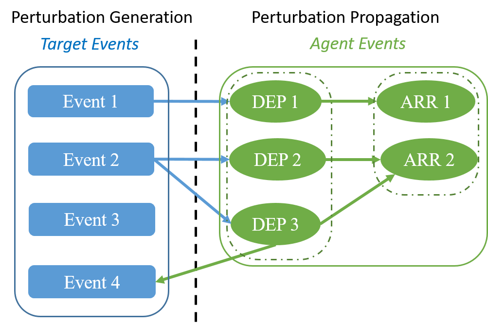
In the following, we will show the derivation of $\nabla R_{i}(t)$ at each event time $\tau_{k}$. To do so, we need to first define all events in this hybrid system which may cause discontinuities in $\nabla R_{i}(t)$. In view of (8), there are four types of “target events” (labeled Event $1$ to $4$) corresponding to $R_{i}(t)$ crossing some threshold value from above/below, reaching the value $R_{i}(t)=0$ from above or leaving the value $R_{i}(t)=0$. In our parametric control problem P2, each agent’s movement is controlled by the target thresholds. Therefore, a target event may induce a switch in the agent dynamics (1) through an agent departure event, denoted by DEP, occurring at $t_{a,k}+d_{a,k}$ in (7). In turn, this event will induce this agent’s arrival event at the next node visited, denoted by ARR. The process of how events can induce other events is detailed next and is graphically summarized in Fig. 3.

Figure 3: Event inducing scheme and the corresponding process of perturbation generation and propagation.

For notational simplicity, we use $\downarrow=$ as an operator indicating that the value on its left-hand-side reaches the value on its right-hand-side from above. Similarly, $\uparrow=$ means reaching from below, and $=\uparrow$ means increasing from the value on the right-hand-side. In addition, since the derivative with respect to $\bm{\Theta}$ is updated differently at different entries, we use $p,q,z$ to indicate the $pq$-entry of the parameter $\bm{\Theta}$ of agent $z$.

Event 1: $R_{i}(\tau_{k})\downarrow=\theta_{ii}^{a}$ . In this case, $R_{i}(t)$ reaches the threshold $\theta_{ii}^{a}$ from above. It is an endogenous event and the guard condition is $g_{k}=R_{i}-\theta_{ii}^{a}=0$ in (12). Therefore, the event time derivative with respect to the $pq$-th entry of the parameter $\bm{\Theta}$ of agent $z$ is as follows:

$$(\tau_{k}^{\prime})_{pq}^{z}=\left\{\begin{array}[c]{ll}-\frac{-1+\left(R_{i}^{\prime}(\tau_{k}^{-})\right)_{pq}^{z}}{A_{i}-B_{i}N_{i}(\tau_{k}^{-})}&\text{if }p=q=i,\text{ and }z=a\\ -\frac{\left(R_{i}^{\prime}(\tau_{k}^{-})\right)_{pq}^{z}}{A_{i}-B_{i}N_{i}(\tau_{k}^{-})}&\text{otherwise }\end{array}\right.$$ (15)

Based on (8), this event may induce an agent departure from its current node location which we denote as event DEP1. Through this event, the value of the event time derivative in (15) will be transferred to $R_{i}^{\prime}(t)$ as shown next.

DEP1: Agent departure event 1. In this case, the agent departure is induced by Event $1$. Using (11) and (15), we obtain

$$\left(R_{i}^{\prime}(\tau_{k}^{+})\right)_{pq}^{z}=\left(R_{i}^{\prime}(\tau_{k}^{-})\right)_{pq}^{z}-B_{i}\left(\tau_{k}^{\prime}\right)_{pq}^{z}$$

$$=\left\{\begin{array}[c]{ll}\frac{A_{i}-B_{i}\left(N_{i}(\tau_{k}^{-})-1\right)}{A_{i}-B_{i}N_{i}(\tau_{k}^{-})}\left(R_{i}^{\prime}(\tau_{k}^{-})\right)_{pq}^{z}-\frac{B_{i}}{A_{i}-B_{i}N_{i}(\tau_{k}^{-})}&\\ \qquad\qquad\qquad\qquad\qquad\quad\text{if }p=q=i,\text{ and }z=a&\\ \frac{A_{i}-B_{i}\left(N_{i}(\tau_{k}^{-})-1\right)}{A_{i}-B_{i}N_{i}(\tau_{k}^{-})}\left(R_{i}^{\prime}(\tau_{k}^{-})\right)_{pq}^{z}\quad\text{otherwise}&\end{array}\right.$$ (19)

This agent departure event will eventually induce an arrival event at another target. The value of the event time derivative in (15) will be transferred to this arrival event, therefore, $\tau_{k+1}^{\prime}=\tau_{k}^{\prime}$ because the travel time between any two nodes $i$ and $j$ is fixed and independent of $\bm{\Theta}$. To see this, set $g_{k+1}=g_{k}+c$ where $c$ is a constant determined by the travel time. Through (12), it is obvious that adding a constant after $g_{k}$ does not affect the derivative. Therefore, we can transfer the value of $\tau_{k}^{\prime}$ to $\tau_{k+1}^{\prime}$ (a similar proof can be found in [15] Lemma 2.1).

ARR1: Agent arrival event 1. This is induced by the earlier DEP1 at node $i$, which is again induced by the target event $R_{i}(\tau_{k})\downarrow=\theta_{ii}^{a}$ (Event 1) and we transfer the value of the event time derivative to obtain

$$\left(\tau_{k+1}^{\prime}\right)_{pq}^{z}=\left(\tau_{k}^{\prime}\right)_{pq}^{z}=\left\{\begin{array}[c]{ll}-\frac{-1+\left(R_{i}^{\prime}(\tau_{k}^{-})\right)_{pq}^{z}}{A_{i}-B_{i}N_{i}(\tau_{k}^{-})}\quad\text{if }p=q=i,&\\ \qquad\qquad\qquad\qquad\text{ and }z=a&\\ -\frac{\left(R_{i}^{\prime}(\tau_{k}^{-})\right)_{pq}^{z}}{A_{i}-B_{i}N_{i}(\tau_{k}^{-})}\quad\text{otherwise}&\end{array}\right.$$ (20)

and through (11),

$$\begin{split}&\left(R_{j}^{\prime}(\tau_{k+1}^{+})\right)_{pq}^{z}=\left(R_{j}^{\prime}(\tau_{k+1}^{-})\right)_{pq}^{z}+B_{j}\left(\tau_{k}^{\prime}\right)_{pq}^{z}\\ &=\left\{\begin{array}[c]{ll}\left(R_{j}^{\prime}(\tau_{k+1}^{-})\right)_{pq}^{z}-\frac{B_{j}}{A_{i}-B_{i}N_{i}(\tau_{k}^{-})}\left(\left(R_{i}^{\prime}(\tau_{k}^{-})\right)_{pq}^{z}-1\right)&\\ \qquad\qquad\qquad\qquad\qquad\qquad\text{ if }p=q=i,\text{ and }z=a&\\ \left(R_{j}^{\prime}(\tau_{k+1}^{-})\right)_{pq}^{z}-\frac{B_{j}}{A_{i}-B_{i}N_{i}(\tau_{k}^{-})}\left(R_{i}^{\prime}(\tau_{k}^{-})\right)_{pq}^{z}\quad\text{otherwise}&\end{array}\right.\end{split}$$ (21)

Event 2: $R_{j}(\tau_{k})\uparrow=\theta_{ij}^{a}$ . This event occurs when an agent is at node $i$ and $R_{j}(t)$ at $j\neq i$ exceeds the threshold $\theta_{ij}^{a}$. The event is endogenous and the guard condition in (12) is $g_{k}=R_{j}-\theta_{ij}^{a}=0$. The event time derivative is obtained from (12) as follows:

$$\left(\tau_{k}^{\prime}\right)_{pq}^{z}=\left\{\begin{array}[c]{ll}-\frac{-1+\left(R_{j}^{\prime}(\tau_{k}^{-})\right)_{pq}^{z}}{A_{j}-B_{j}N_{j}(\tau_{k}^{-})}&\text{if }p=i,q=j,\text{and }z=a\\ -\frac{\left(R_{j}^{\prime}(\tau_{k}^{-})\right)_{pq}^{z}}{A_{j}-B_{j}N_{j}(\tau_{k}^{-})}&\text{otherwise }\end{array}\right.$$ (22)

Looking at (8), this event can induce an agent departure event depending on whether $R_{i}(\tau_{k})>0$ or not: in the former case, the event is denoted by DEP2 and in the latter it is denoted by DEP3. The value of the derivative in (22) will be transferred to $R_{i}^{\prime}(t)$ through one of these agent departure events.

DEP2: Agent departure event 2. In this case, $R_{i}(\tau_{k})>0$. Using (11) and the event time derivative in (22), we obtain

$$\left(R_{i}^{\prime}(\tau_{k}^{+})\right)_{pq}^{z}=\left(R_{i}^{\prime}(\tau_{k}^{-})\right)_{pq}^{z}-B_{i}\left(\tau_{k}^{\prime}\right)_{pq}^{z}$$

$$=\left\{\begin{array}[c]{ll}\left(R_{i}^{\prime}(\tau_{k}^{-})\right)_{pq}^{z}+\frac{B_{i}}{A_{j}-B_{j}N_{j}(\tau_{k}^{-})}\left(\left(R_{i}^{\prime}(\tau_{k}^{-})\right)_{pq}^{z}-1\right)&\\ \qquad\qquad\qquad\qquad\qquad\quad\text{ if }p=i,q=j,\text{and }z=a&\\ \left(R_{i}^{\prime}(\tau_{k}^{-})\right)_{pq}^{z}+\frac{B_{i}}{A_{j}-B_{j}N_{j}(\tau_{k}^{-})}\left(R_{i}^{\prime}(\tau_{k}^{-})\right)_{pq}^{z}\quad\text{otherwise }&\end{array}\right.$$ (26)

DEP3: Agent departure event 3. This event is complementary to DEP2 where the agent departure is induced by Event $2$ but $R_{i}(\tau_{k})=0$. Based on (1), the target dynamics after this event either remain $\dot{R}_{i}(t)=0$ or switch to $\dot{R}_{i}(t)=A_{i}-B_{i}N_{i}(\tau_{k}^{+})$ depending on whether $A_{i}>B_{i}N_{i}(\tau_{k}^{+})$ or not. Thus, there are two sub-cases to consider as follows.

DEP3-1: $A_{i}>B_{i}N_{i}(\tau_{k}^{+})$. In this sub-case, the target dynamics switch from $\dot{R}_{i}(t)=0$ for $t\in[\tau_{k-1},\tau_{k})$ to $\dot{R}_{i}(t)=A_{i}-B_{i}N_{i}(t)$ for $t\in[\tau_{k},\tau_{k+1})$. We know $R_{i}^{\prime}(\tau_{k}^{-})=0$ because $R_{i}(\tau_{k})=0$ before the agent departure and the value $R_{i}^{\prime}(t)=0$ holds as long as $R_{i}(t)=0$. Using (11) and the event time derivative in (22), we obtain

$$\left(R_{i}^{\prime}(\tau_{k}^{+})\right)_{pq}^{z}=-(A_{i}-B_{i}N_{i}(\tau_{k}^{+}))\left(\tau_{k}^{\prime}\right)_{pq}^{z}$$

$$=\left\{\begin{array}[c]{ll}\frac{A_{i}-B_{i}N_{i}(\tau_{k}^{+})}{A_{j}-B_{j}N_{j}(\tau_{k}^{-})}\left(\left(R_{j}^{\prime}(\tau_{k}^{-})\right)_{pq}^{z}-1\right)\quad\text{if }p=i,q=j,&\\ \qquad\qquad\qquad\qquad\qquad\qquad\qquad\quad\text{ and }z=a&\\ \frac{A_{i}-B_{i}N_{i}(\tau_{k}^{+})}{A_{j}-B_{j}N_{j}(\tau_{k}^{-})}\left(R_{j}^{\prime}(\tau_{k}^{-})\right)_{pq}^{z}\qquad\qquad\text{otherwise }&\end{array}\right.$$ (30)

DEP3-2: $A_{i}\leq B_{i}N_{i}(\tau_{k}^{+})$. In this sub-case, the target dynamics remain $\dot{R}_{i}(t)=0$ before and after the event at $\tau_{k}$. Therefore, the state dynamics in (11) satisfy $f_{k-1}(\tau_{k}^{-})=f_{k}(\tau_{k}^{+})$ and we have

$$R_{i}^{\prime}(\tau_{k}^{+})=0\quad\text{for all }p,q,z\\$$ (31)

Remark 3.

Note that DEP3-1 induces another target event (Event $4$) since $R_{i}(t)$ increases after the agent’s departure. Moreover, both DEP2 and DEP3 will induce an agent arrival event at the next visiting target.

ARR2: Agent arrival event 2. This event is induced by an earlier agent departure event at a target $i$ which is again induced by the previous Event 2 $R_{j}(\tau_{k})\uparrow=\theta_{ij}^{a}$. Similar to the derivation in ARR1, we transfer the prior event time derivative value to the current arrival time derivative:

$$\left(\tau_{k+1}^{\prime}\right)_{pq}^{z}=\left(\tau_{k}^{\prime}\right)_{pq}^{z}=\left\{\begin{array}[c]{ll}-\frac{-1+\left(R_{j}^{\prime}(\tau_{k}^{-})\right)_{pq}^{z}}{A_{j}-B_{j}N_{j}(\tau_{k}^{-})}\quad\text{if }p=i,q=j,&\\ \qquad\qquad\qquad\qquad\quad\text{ and }z=a&\\ -\frac{\left(R_{j}^{\prime}(\tau_{k}^{-})\right)_{pq}^{z}}{A_{j}-B_{j}N_{j}(\tau_{k}^{-})}\qquad\text{otherwise }&\end{array}\right.$$ (32)

Through (11) we obtain

$$\begin{split}&\left(R_{j}^{\prime}(\tau_{k+1}^{+})\right)_{pq}^{z}=\left(R_{j}^{\prime}(\tau_{k+1}^{-})\right)_{pq}^{z}+B_{j}\left(\tau_{k}^{\prime}\right)_{pq}^{z}\\ &=\left\{\begin{array}[c]{ll}\left(R_{j}^{\prime}(\tau_{k+1}^{-})\right)_{pq}^{z}-\frac{B_{j}}{A_{j}-B_{j}N_{j}(\tau_{k}^{-})}\left(\left(R_{j}^{\prime}(\tau_{k}^{-})\right)_{pq}^{z}-1\right)&\\ \qquad\qquad\qquad\qquad\qquad\quad\text{ if }p=i,q=j,\text{ and }z=a&\\ \left(R_{j}^{\prime}(\tau_{k+1}^{-})\right)_{pq}^{z}-\frac{B_{j}}{A_{j}-B_{j}N_{j}(\tau_{k}^{-})}\left(R_{j}^{\prime}(\tau_{k}^{-})\right)_{pq}^{z}\text{ otherwise}&\end{array}\right.\end{split}$$ (33)

Notice here that $\tau_{k}$ is the prior agent departure time and $\tau_{k+1}$ is the current agent arrival time and the derivatives $R_{j}^{\prime}(\tau_{k+1}^{-})$ and $R_{j}^{\prime}(\tau_{k}^{-})$ can be different since $R_{j}^{\prime}(\tau_{k}^{-})$ may change due to arrivals or departures of other agents during $[\tau_{k},\tau_{k+1})$.

Event 3: $R_{i}(t)\downarrow=0$. This event corresponds to the target uncertainty state reaching zero from above, therefore from (1) the target state dynamics switch from $\dot{R}_{i}(t)=A_{i}-B_{i}N_{i}(t),$ $t\in[\tau_{k-1},\tau_{k})$ to $\dot{R}_{i}(t)=0,$ $t\in[\tau_{k},\tau_{k+1})$. It is an endogenous event that occurs when $g_{k}(x,\theta)=R_{i}=0$. According to (12),

$$\left(\tau_{k}^{\prime}\right)_{pq}^{z}=-\frac{\left(R_{i}^{\prime}(\tau_{k}^{-})\right)_{pq}^{z}}{A_{i}-B_{i}N_{i}(\tau_{k}^{-})}$$ (34)

Replacing $\tau_{k}^{\prime}$ in (11) with the result in (34), we have

$$\left(R_{i}^{\prime}(\tau_{k}^{+})\right)_{pq}^{z}= \left(R_{i}^{\prime}(\tau_{k}^{-})\right)_{pq}^{z}+\left(A_{i}-B_{i}N_{i}(\tau_{k}^{-})\right)\left(\tau_{k}^{\prime}\right)_{pq}^{z}=0$$

$$\qquad\qquad\qquad\qquad\qquad\text{ for all }p,q,z$$ (35)

This indicates that $\nabla R_{i}(t)$ is always reset to $0$ whenever the target’s uncertainty state is reduced to zero. This is an uncontrollable event and does not induce any other event.

Event 4: $R_{i}(t)=\uparrow 0$. In this case, the target value leaves zero and the dynamics in (1) switch from $\dot{R}_{i}(t)=0,$ $t<\tau_{k}$ to $\dot{R}_{i}(t)=A_{i}-B_{i}N_{i}(t),$ $t\geq\tau_{k}$. This event is induced by an agent departure event (DEP3) which is in turn induced by Event $2$. This is an exogenous event functioning only as an indicator of $R_{i}(t)$ increasing from zero. Therefore, $\tau_{k}^{\prime}=0$ and the derivative $R_{i}^{\prime}(t)$ will not be affected.

Remark 4.

The analysis of Events $1$ to $4$ shows that all non-zero gradient values are caused by target events and then propagated through the various agent departure and arrival events.

IPA-based gradient descent algorithm Once we have derived the gradient $\nabla J(\bm{\Theta})$ in (13), we update the parameter $\bm{\Theta}$ based on a standard gradient descent scheme as follows.

$$\bm{\Theta}^{(l+1)}=\Pi\left[\bm{\Theta}^{(l)}-\beta^{l}\nabla J(\bm{\Theta}^{(l)})\right]$$ (36)

where the operator $\Pi\equiv\max\{\bm{\cdot},\bm{0}\}$, $l$ indexes the number of iterations, and $\beta^{l}$ is a diminishing step-size sequence satisfying $\sum_{l=0}^{\infty}\beta^{l}=\infty$ and $\lim_{l\rightarrow\infty}\beta^{l}=0$.

IV One-agent case analysis

Recalling our control policy in (8), the diagonal entries in the parameter matrix control the dwell times at nodes, whereas the off-diagonal entries control the feasible node visiting sequence. In what follows, we will show that in a single-agent case the optimal values of diagonal entries in (37) are always zero. This structural property indicates that the agent visiting a node should always reduce the uncertainty state to zero before moving to the next node.

Ignoring the superscript agent index, the single-agent threshold matrix is written as

$$\bm{\Theta}=\begin{bmatrix}\theta_{11}&\theta_{12}&\theta_{13}&\dots&\theta_{1M}\\ \theta_{21}&\theta_{22}&\theta_{23}&\dots&\theta_{2M}\\ \vdots&\vdots&\vdots&\ddots&\vdots\\ \theta_{M1}&\theta_{M2}&\theta_{M3}&\dots&\theta_{MM}\end{bmatrix}$$ (37)

Assumption 1.

For any $\epsilon>0$, there exists a finite time horizon $T>t_{K}-\frac{c}{1-\epsilon}$ where $t_{K}$ is such that $\|\nabla R_{i}(t_{1})-\nabla R_{i}(t_{2})\|\leq\epsilon/M$, $i=1,\ldots,M$ for all $t_{1},t_{2}>t_{K}$ and $c$ is a finite constant.

Assumption 2.

The current node visiting sequence is optimal.

The first assumption is a technical one and it ensures that the optimization problem is defined over a sufficiently long time horizon $T$ to allow the gradient to converge. The second assumption allows us to reduce the parameter matrix (37) to a vector of its diagonal elements only:

$$\Theta_{d}=\left[\theta_{1},\theta_{2},\ldots,\theta_{M}\right]^{\top}\geq\mathbf{0}_{M\times 1}.$$ (38)

Theorem 1.

Consider $M$ targets and a single agent under the parametric control $\Theta_{d}$. The optimal thresholds satisfy $\Theta_{d}^{\star}=\mathbf{0}_{M\times 1}$.

Proof. To establish the proof, we will show that the derivative $\partial J(\Theta_{d})/\partial\theta_{i}$ satisfies $\partial J(\Theta_{d})/\partial\theta_{i}>0$ for every $i=1,\ldots,M$. As a result, through the parameter update scheme (36), $\Theta_{d}$ will eventually be reduced to $\mathbf{0}$. First, for every element $\theta_{i}$ in $\Theta_{d}$, we have

$$\frac{\partial J(\Theta_{d})}{\partial\theta_{i}}=\frac{1}{T}\int_{t=0}^{T}\sum_{m=1}^{M}\frac{\partial R_{m}}{\partial\theta_{i}}\,dt$$ (39)

The value of the integrand over time is given by the IPA results in Sec. III as follows:

Agent departures. In the single-agent case, all agent departure events are of type DEP1. From (19), the IPA derivatives with respect to each element in $\Theta_{d}$ after such events are:

$$\left\{\begin{split}&\frac{\partial R_{i}}{\partial\theta_{i}}(\tau_{k}^{+})=\frac{A_{i}}{A_{i}-B_{i}}\frac{\partial R_{i}}{\partial\theta_{i}}(\tau_{k}^{-})-\frac{B_{i}}{A_{i}-B_{i}}\\ &\frac{\partial R_{i}}{\partial\theta_{j}}(\tau_{k}^{+})=\frac{A_{i}}{A_{i}-B_{i}}\frac{\partial R_{i}}{\partial\theta_{j}}(\tau_{k}^{-})\quad\text{ for }j\neq i\end{split}\right.$$ (40)

Agent arrivals. An agent arrival event at node $i$ is induced by the earlier DEP1 event at some previously visited node $j\neq i$. According to (21), the IPA derivatives are:

$$\left\{\begin{split}&\frac{\partial R_{i}}{\partial\theta_{j}}(\tau_{k}^{+})=\frac{\partial R_{i}}{\partial\theta_{j}}(\tau_{k}^{-})-\frac{B_{i}}{A_{j}-B_{j}}\left(\frac{\partial R_{j}}{\partial\theta_{j}}(\tau_{k}^{-})-1\right)\\ &\qquad\qquad\qquad\qquad\qquad\qquad\text{where $j$ is the prior node}\\ &\frac{\partial R_{i}}{\partial\theta_{l}}(\tau_{k}^{+})=\frac{\partial R_{i}}{\partial\theta_{l}}(\tau_{k}^{-})-\frac{B_{i}}{A_{j}-B_{j}}\frac{\partial R_{j}}{\partial\theta_{l}}(\tau_{k}^{-})\text{ for }l\neq j\end{split}\right.$$ (41)

To simplify the notation, we set

$$\nabla R_{i}(t)=\left[\frac{\partial R_{i}}{\partial\theta_{1}},\frac{\partial R_{i}}{\partial\theta_{2}},\ldots,\frac{\partial R_{i}}{\partial\theta_{M}}\right]^{\top}$$ (42)

and

$$\nabla R(t)=\left[\nabla R_{1},\nabla R_{2},\ldots,\nabla R_{M}\right]^{\top}.$$ (43)

The evolution of the gradient vector $\nabla R(t)$ follows a system of linear equations in (40) and (41) for each node $i$. Solving this system of equations, we obtain the only possible equilibrium for every node $i=1,\dots,M$:

$$\frac{\partial R_{i}}{\partial\theta_{i}}=1\text{ and }\frac{\partial R_{i}}{\partial\theta_{j}}=0\text{ for }j\neq i$$ (44)

Using Assumption 1, for any $0<\epsilon<1$, there exists a $t_{K}$ such that $\|\frac{\partial R_{i}}{\partial\theta_{i}}(t_{K})-1\|<\epsilon/M$ for all $i=1,\ldots,M$ and $\|\frac{\partial R_{i}}{\partial\theta_{j}}(t_{K})\|<\epsilon/M$ for all $i\neq j$. We now rewrite (39) with the integral separated into two parts over $[0,T]$ as follows:

$$\frac{\partial J(\Theta_{d})}{\partial\theta_{i}}=\frac{1}{T}\left(\int_{t=0}^{t_{K}}\sum_{m=1}^{M}\frac{\partial R_{m}(t)}{\partial\theta_{i}}dt+\int_{t_{K}}^{T}\sum_{m=1}^{M}\frac{\partial R_{m}(t)}{\partial\theta_{i}}dt\right)$$

The first integral above corresponds to the transient stage before $t_{K}$ and there exists some constant $c$ whose value is smaller that this integral so that

$$\begin{split}\frac{\partial J(\Theta_{d})}{\partial\theta_{i}}&\geq\frac{1}{T}\left(c+\int_{t_{K}}^{T}\sum_{m=1}^{M}\frac{\partial R_{m}(t)}{\partial\theta_{i}}dt\right)\\ &=\frac{1}{T}\left(c+\int_{t_{K}}^{T}\left[\frac{\partial R_{i}(t)}{\partial\theta_{i}}+\sum_{m\neq i}\frac{\partial R_{m}(t)}{\partial\theta_{i}}\right]dt\right)\\ &=\frac{1}{T}\left(c+\int_{t_{K}}^{T}dt+\int_{t_{K}}^{T}\left[\frac{\partial R_{i}(t)}{\partial\theta_{i}}-1+\sum_{m\neq i}\frac{\partial R_{m}(t)}{\partial\theta_{i}}\right]dt\right)\\ &\geq\frac{1}{T}\left(c\!+\!T\!-\!t_{K}-\int_{t_{K}}^{T}\!\|\frac{\partial R_{i}(t)}{\partial\theta_{i}}-1\|+\sum_{m\neq i}\|\frac{\partial R_{m}(t)}{\partial\theta_{i}}\|dt\right)\\ &\geq\frac{1}{T}\left(c+T-t_{K}-\int_{t_{K}}^{T}\epsilon/M+(M-1)\epsilon/M\,dt\right)\\ &=\frac{1}{T}\left(c+\left(1-\epsilon\right)(T-t_{K})\right)\end{split}$$ (45)

Therefore, as long as $T>t_{K}-\frac{c}{1-\epsilon}$, we have $\frac{\partial J(\Theta_{d})}{\partial\theta_{i}}>0$ regardless of the value of $\Theta_{d}$. Through (36), $\theta_{i}$ for every node $i$ will eventually be reduced to the optimal value zero. $\blacksquare$

Remark 5.

The result of Theorem 1 is consistent with, but more general than, a similar result in [13] where homogeneous targets are assumed ($A_{i}=A$ and $B_{i}=B$ for all node $i$). The convergence of $\nabla R(t)$ is related to the coefficients $A_{i}$ and $B_{i}$, $i=1,\ldots,M$. From elementary queueing theory, a basic requirement for stability is $A_{i}<B_{i}$ for each node, which in turn implies the existence of $t_{K}$ in Assumption 1. Moreover, if $T$ is sufficiently large and $\epsilon$ is arbitrarily small, $\lim_{T\rightarrow\infty}\frac{\partial J(\Theta_{d})}{\partial\theta_{m}}\rightarrow 1$ .

V Simulation Examples

One agent, two targets. We provide a simple one-agent example to illustrate Theorem 1. Consider a controller with parameter vector $\Theta_{d}=\left[\theta_{1},\theta_{2}\right]^{\top}$. We track the evolution of $\nabla R(t)=\left[\frac{\partial R_{1}}{\partial\theta_{1}},\frac{\partial R_{1}}{\partial\theta_{2}},\frac{\partial R_{2}}{\partial\theta_{1}},\frac{\partial R_{2}}{\partial\theta_{2}}\right]^{\top}$ event by event.

V-1 If the agent departs from target $1$

$$\nabla R(\tau_{k}^{d_{1}^{+}})=\begin{bmatrix}\frac{A_{1}}{A_{1}-B_{1}}&0&0&0\\ 0&\frac{A_{1}}{A_{1}-B_{1}}&0&0\\ 0&0&1&0\\ 0&0&0&1\end{bmatrix}\nabla R(\tau_{k}^{d_{1}^{-}})+\begin{bmatrix}\frac{B_{1}}{B_{1}-A_{1}}\\ 0\\ 0\\ 0\end{bmatrix}$$

For notational simplicity, denote the update matrix and update vector by $\Lambda_{1}$ and $U_{1}$ respectively. We can write

$$\nabla R(\tau_{k}^{d_{1}^{+}})=\Lambda_{1}\nabla R(\tau_{k}^{d_{1}^{-}})+U_{1}$$ (46)

V-2 If the agent arrives at target $2$

$$\nabla R(\tau_{k}^{a_{2}^{+}})=\begin{bmatrix}1&0&0&0\\ 0&1&0&0\\ \frac{B_{2}}{B_{1}-A_{1}}&0&1&0\\ 0&\frac{B_{2}}{B_{1}-A_{1}}&0&1\end{bmatrix}\nabla R(\tau_{k}^{a_{2}^{-}})+\begin{bmatrix}0\\ 0\\ \frac{B_{2}}{A_{1}-B_{1}}\\ 0\end{bmatrix}$$

We denote this update by

$$\nabla R(\tau_{k}^{a_{2}^{+}})=\Lambda_{2}\nabla R(\tau_{k}^{a_{2}^{-}})+U_{2}$$ (47)

V-3 If the agent departs from target $2$

$$\nabla R(\tau_{k}^{d_{2}^{+}})=\begin{bmatrix}1&0&0&0\\ 0&1&0&0\\ 0&0&\frac{A_{2}}{A_{2}-B_{2}}&0\\ 0&0&0&\frac{A_{2}}{A_{2}-B_{2}}\end{bmatrix}\nabla R(\tau_{k}^{d_{2}^{-}})+\begin{bmatrix}0\\ 0\\ 0\\ \frac{B_{2}}{B_{2}-A_{2}}\end{bmatrix}$$

We denote this update by

$$\nabla R(\tau_{k}^{d_{2}^{+}})=\Lambda_{3}\nabla R(\tau_{k}^{d_{2}^{-}})+U_{3}$$ (48)

V-4 If the agent arrives at target $1$

$$\nabla R(\tau_{k}^{a_{1}^{+}})=\begin{bmatrix}1&0&\frac{B_{1}}{B_{2}-A_{2}}&0\\ 0&1&0&\frac{B_{1}}{B_{2}-A_{2}}\\ 0&0&1&0\\ 0&0&0&1\end{bmatrix}\nabla R(\tau_{k}^{a_{1}^{-}})+\begin{bmatrix}0\\ \frac{B_{1}}{A_{2}-B_{2}}\\ 0\\ 0\end{bmatrix}$$

We denote this update by

$$\nabla R(\tau_{k}^{a_{1}^{+}})=\Lambda_{4}\nabla R(\tau_{k}^{a_{1}^{-}})+U_{4}$$ (49)

We initialize the agent at target $1$. The agent goes to target $2$ and back to target $1$ so on so forth according to controller $\Theta_{d}=[\theta_{1},\theta_{2}]^{\top}$. In each visiting cycle (from case 1 to case 4), $\nabla R(t)$ is updated following the order from (46)-(49). We use $T_{k}$ to denote the beginning of the $k$-th cycle, and obtain

$$\begin{split}\nabla R(T_{k+1}^{-})\!=\!&\Lambda_{4}\!\left(\Lambda_{3}\!\left(\Lambda_{2}\!\left(\Lambda_{1}\!\nabla R(T_{k}^{-})+\!U_{1}\right)+U_{2}\right)+U_{3}\right)\!+\!U_{4}\\ =&\Lambda_{4}\Lambda_{3}\Lambda_{2}\Lambda_{1}\nabla R(T_{k}^{-})+\Lambda_{4}\Lambda_{3}\Lambda_{2}U_{1}+\Lambda_{4}\Lambda_{3}U_{2}\\ &+\Lambda_{4}U_{3}+U_{4}\\ =&\Lambda\nabla R(T_{k}^{-})+U\end{split}$$ (50)

where $\Lambda=\Lambda_{4}\Lambda_{3}\Lambda_{2}\Lambda_{1}$ and $U=\Lambda_{4}\Lambda_{3}\Lambda_{2}U_{1}+\Lambda_{4}\Lambda_{3}U_{2}+\Lambda_{4}U_{3}+U_{4}$ and the initial value $\nabla R(T_{0})=[0,0,0,0]^{\top}$.

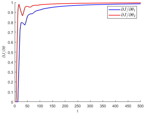
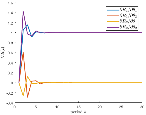
Solving $\nabla R_{e}=(I-\Lambda)^{-1}U$, we obtain the only equilibrium $\nabla R_{e}=[1,0,0,1]^{\top}$ of the system (50). $\nabla R(t)$ converges to that equilibrium asymptotically (see Fig. 5). The result matches with our analysis in the proof of Theorem 1. Moreover, convergence to the equilibrium simply requires the eigenvalues of $\Lambda$ in (50) lie within the unit circle of the complex plane.

If the two targets are homogeneous ($A=A_{1}=A_{2}$ and $B=B_{1}=B_{2}$), the convergence of $\nabla R(t)$ is only determined by the ratio $\rho=A/B$. Using this ratio, we solve the eigenvalues of the system in (50) and obtain

$$\bm{\lambda}=\begin{bmatrix}\frac{2\rho^{4}-6\rho^{3}+7\rho^{2}-2\rho+\sqrt{\rho^{3}(2\rho-1)(2\rho^{2}-5\rho+4)}}{2(\rho-1)^{4}}\\ \frac{2\rho^{4}-6\rho^{3}+7\rho^{2}-2\rho+\sqrt{\rho^{3}(2\rho-1)(2\rho^{2}-5\rho+4)}}{2(\rho-1)^{4}}\\ \frac{2\rho^{4}-6\rho^{3}+7\rho^{2}-2\rho-\sqrt{\rho^{3}(2\rho-1)(2\rho^{2}-5\rho+4)}}{2(\rho-1)^{4}}\\ \frac{2\rho^{4}-6\rho^{3}+7\rho^{2}-2\rho-\sqrt{\rho^{3}(2\rho-1)(2\rho^{2}-5\rho+4)}}{2(\rho-1)^{4}}\end{bmatrix}$$ (51)

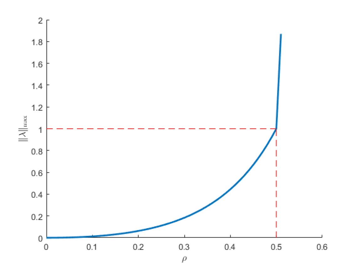
Figure 4 shows the largest norm eigenvalue $\|\lambda\|_{\max}$ increases monotonically as $\rho$ increases and that $\|\lambda\|_{\max}=1$ at $\rho=1/2$. The convergence of $\nabla R(t)$ requires $\rho<1/2$.

Figure 4: Monotonic increasing of $\|\lambda\|_{\max}$ as the increase of $\rho$.

Setting $\rho=0.3$, we verify the convergence of both $\nabla R(t)$ and $\partial J/\partial\Theta_{d}$ as shown in Fig.5. The results match with our analysis in Theorem 1.

Figure 5: Top plot: convergence of $\nabla R(t)$ to the equilibrium $[1,0,0,1]^{\top}$. Bottom plot: convergence of $\partial J/\partial\Theta_{d}$ to $[1,1]^{\top}$.

Multi-agent cases: a counterexample to Theorem 1. Theorem $1$ asserts that an agent visiting a node should reduce the uncertainty state to zero before moving to the next node. This property, however, does not apply to multi-agent cases. This is not surprising because when two or more agents are visiting a node, the allocation of agents to nodes may be improved if one agent leaves the node before reducing its uncertainty state to zero and allow other agents to complete this task.

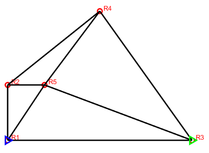
Here we present a counterexample to Theorem 1 using two agents and five nodes (see Fig. 6). Agents are initialized at nodes 1 and 3 respectively and nodes are located at $X_{1}=(0,0)$, $X_{2}=(0,3)$, $X_{3}=(10,0)$, $X_{4}=(5,7)$, $X_{5}=(2,3)$ with uncertainty states $R_{i}(0)=0.5,A_{i}=1,B_{i}=10$ for $i=1,\ldots,5$. The initial thresholds are listed as follows:

$$(\Theta^{1})^{0}=\begin{bmatrix}16.34&5.31&5.18&1.74&0.72\\ 2.87&1.02&18.56&22.13&24.55\\ 23.76&9.93&9.80&23.82&8.49\\ 12.05&5.83&4.56&23.28&17.67\\ 21.81&21.04&18.59&10.39&9.05\end{bmatrix}$$

$$(\Theta^{2})^{0}=\begin{bmatrix}0.88&22.13&3.33&10.81&22.28\\ 21.38&22.60&17.45&0.45&22.96\\ 16.43&0.26&9.96&17.29&1.83\\ 19.14&1.86&22.08&11.74&1.14\\ 13.85&6.12&4.53&3.21&10.96\end{bmatrix}$$

Figure 6: An counter example with 2 homogeneous agents and 5 nodes to show $\theta_{ii}^{a*}>0$ for some agent $a$.

The final thresholds after convergence of (36), in this case 300 iterations, are as follows:

$$(\Theta^{1})^{300}=\begin{bmatrix}0&2.38&5.18&1.74&0\\ 5.70&0&18.56&23.76&23.94\\ 23.76&9.93&7.25&23.82&8.51\\ 12.05&5.83&4.56&8.06&17.67\\ 21.70&21.04&20.09&16.07&0.23\end{bmatrix}$$

$$(\Theta^{2})^{300}=\begin{bmatrix}0.88&22.13&3.33&10.81&22.24\\ 21.37&19.27&17.45&0.17&25.24\\ 16.44&1.15&0.02&15.23&2.21\\ 19.14&1.86&22.08&0.01&0.87\\ 13.85&6.12&2.27&2.21&0.00\end{bmatrix}$$

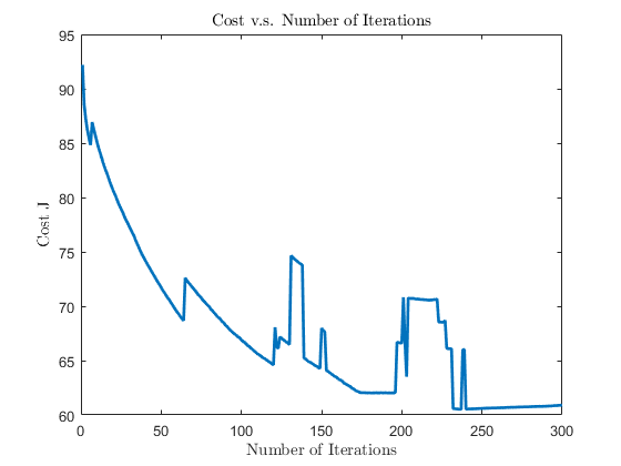
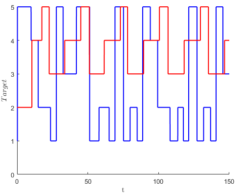
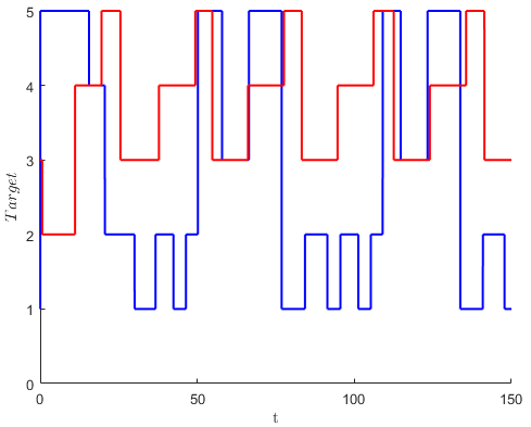
The diagonal entries of the final parameter matrices for both agents are: $\Theta_{d}^{1\ast}=[0,0,7.25,8.06,0.23]^{\top}$ and $\Theta_{d}^{2\ast}=[0.88,19.27,0.02,0.01,0]^{\top}$ which do not satisfy the structure given in Theorem $1$ as opposed to one-agent cases. In addition, the target visiting sequences are adjusted on line during the optimization process. For instance, the visiting sequence of agent $1$ is adjusted from initially being $1-5-4-2-1-5-\ldots$ to $1-5-4-2-1-2-\ldots$ after 300 iterations as shown in Fig. 7. Since agents may adjust their visiting sequences asynchronously, the cost in the multi-agent cases may fluctuate during the optimization process as shown in Fig. 8

Figure 7: Left plot: the visiting sequence under the initial parameter. Right plot: the sequence under the optimized parameters after 300 iterations of gradient descent. In both plots, blue lines indicate the sequence of agent 1 and red lines indicate the sequence of agent 2.

Figure 8: Cost versus the number of iterations for the example of 2 agents and 5 nodes.

Threshold-based policy versus dynamic programming. We present a small example to compare the performance of the threshold-based policy with a classical dynamic programming solution of (3) adapted to the graph topology using value iteration.

A single agent is initialized at $(0,0)$ to persistently monitor four targets located at $X_{1}=(0,0)$, $X_{2}=(4,0)$, $X_{3}=(4,4)$, $X_{4}=(0,4)$ (see Fig. 2) for $T=100$ seconds. The parameters in the uncertainty dynamics (1) are $A_{i}=1$, $B_{i}=20$, for $i=1,\ldots,4$ and initial values are $R_{1}(0)=19,R_{2}(0)=14,R_{3}(0)=9$ and $R_{4}(0)=4$. Using dynamic programming, the value function converges after $15$ iterations and the final cost is $J_{\text{DP}}^{\star}=31.15$. However, the number of states in the system consisting of 1 agent and 4 targets $(\mathbf{s}(t),\mathbf{R}(t))$ is about $2.5\ast 10^{9}$ discretized by integers over 100 seconds. The running time is about 16 minutes per value iteration using a computer with Intel(R) Core(TM) i7-7700 CPU @3.60GHZ processor. Obviously, this method does not scale well in the number of states. On the other hand, the solution obtained by optimizing the threshold-based policy using the IPA approach is slightly higher, but the computational complexity is reduced by several orders of magnitude as shown in Fig. 9. After 300 iterations of gradient descent through (36) (about 30 seconds in total running time on the same computer), the cost is reduced to $J_{\text{IPA}}^{\star}=36.20$.

Figure 9: Cost versus computational time (in log scale). The blue line shows the result of IPA with the final cost $J^{\star}_{\text{IPA}}=36.20$ and the orange line shows the result of dynamic programming with the final cost $J^{\star}_{\text{DP}}=31.15$ .

VI Conclusions

The optimal multi-agent persistent monitoring problem involves the planning of agent trajectories defined both by the sequence of nodes (targets) to be visited and the amount of time spent by agents at each node. We have considered a class of distributed parametric controllers through which the agents control their visit sequence and dwell times at nodes using threshold parameters associated with the node uncertainty states. We use Infinitesimal Perturbation Analysis (IPA) to determine on line (locally) optimal threshold parameters through gradient descent methods and thus obtain optimal controllers within this family of threshold-based policies. In the one-agent case we show the optimal strategy is for the agent to reduce the uncertainty of a node to zero before moving to the next node. Compared with dynamic programming solutions (in the limited instances when these are feasible), our threshold-based parametric controller is effective and the computational complexity is reduced by orders of magnitude. In future work, richer families of threshold-based controllers can be developed by considering multi-step-look-ahead policies and by identifying structural properties therein which give us insight to the trade-off between exploitation and exploration over multiple steps in persistent monitoring tasks.

References

• [1] W. Ren, R. W. Beard, and E. M. Atkins, “A survey of consensus problems in multi-agent coordination,” in Proc. of the American Control Conference.   IEEE, 2005, pp. 1859–1864.
• [2] M. Zhong and C. G. Cassandras, “Distributed coverage control and data collection with mobile sensor networks,” IEEE Trans. on Automatic Control, vol. 56, no. 10, pp. 2445–2455, 2011.
• [3] N. Michael, E. Stump, and K. Mohta, “Persistent surveillance with a team of mavs,” in Proc. IEEE/RSJ Intl. Conf. Intelligent Robots Systems, 2011, pp. 2708–2714.
• [4] N. E. Leonard, D. A. Paley, R. E. Davis, D. M. Fratantoni, F. Lekien, and F. Zhang, “Coordinated control of an underwater glider fleet in an adaptive ocean sampling field experiment in monterey bay,” Journal of Field Robotics, vol. 27, no. 6, pp. 718–740, 2010.
• [5] T. T. Ashley, E. L. Gan, J. Pan, and S. B. Andersson, “Tracking single fluorescent particles in three dimensions via extremum seeking,” Biomedical optics express, vol. 7, no. 9, pp. 3355–3376, 2016.
• [6] S. M. Cromer Berman, P. Walczak, and J. W. Bulte, “Tracking stem cells using magnetic nanoparticles,” Wiley Interdisciplinary Reviews: Nanomedicine and Nanobiotechnology, vol. 3, no. 4, pp. 343–355, 2011.
• [7] S. L. Smith, M. Schwager, and D. Rus, “Persistent Robotic Tasks: Monitoring and Sweeping in Changing Environments,” IEEE Trans. on Robotics, vol. 28, no. 2, pp. 410–426, Apr. 2012.
• [8] X. Lin and C. G. Cassandras, “An optimal control approach to the multi-agent persistent monitoring problem in two-dimensional spaces,” IEEE Trans. on Automatic Contr., vol. 60, no. 6, pp. 1659–1664, 2015.
• [9] N. Zhou, X. Yu, S. B. Andersson, and C. G. Cassandras, “Optimal event-driven multi-agent persistent monitoring of a finite set of targets,” in Proc. IEEE Conference on Decision and Control, 2016, pp. 1814–1819.
• [10] N. Zhou, C. G. Cassandras, X. Yu, and S. B. Andersson, “Optimal event-driven multi-agent persistent monitoring with graph-limited mobility,” in To appear in IFAC World Congress, 2017.
• [11] M. Lahijanian, J. Wasniewski, S. B. Andersson, and C. Belta, “Motion planning and control from temporal logic specifications with probabilistic satisfaction guarantees,” in Proc. IEEE Intl. Conf. on Robotics and Automation, 2010, pp. 3227–3232.
• [12] C. G. Cassandras, X. Lin, and X. Ding, “An optimal control approach to the multi-agent persistent monitoring problem,” IEEE Trans. on Automatic Control, vol. 58, no. 4, pp. 947–961, 2013.
• [13] X. Yu, S. B. Andersson, N. Zhou, and C. G. Cassandras, “Optimal dwell times for persistent monitoring of a finite set of targets,” in Proc. American Control Conference (ACC), 2017, pp. 5544–5549.
• [14] T. Bektas, “The multiple traveling salesman problem: an overview of formulations and solution procedures,” Omega, vol. 34, no. 3, pp. 209–219, 2006.
• [15] C. G. Cassandras, Y. Wardi, C. G. Panayiotou, and C. Yao, “Perturbation analysis and optimization of stochastic hybrid systems,” European Journal of Control, vol. 16, no. 6, pp. 642–661, 2010.