Testing the equivalence principle on cosmological scales
Abstract
The equivalence principle, that is one of the main pillars of general relativity, is very well tested in the Solar system; however, its validity is more uncertain on cosmological scales, or when dark matter is concerned. This article shows that relativistic effects in the large-scale structure can be used to directly test whether dark matter satisfies Euler’s equation, i.e. whether its free fall is characterised by geodesic motion, just like baryons and light. After having proposed a general parametrisation for deviations from Euler’s equation, we perform Fisher-matrix forecasts for future surveys like DESI and the SKA, and show that such deviations can be constrained with a precision of order 10%. Deviations from Euler’s equation cannot be tested directly with standard methods like redshift-space distortions and gravitational lensing, since these observables are not sensitive to the time component of the metric. Our analysis shows therefore that relativistic effects bring new and complementary constraints to alternative theories of gravity.
1 Introduction
Physical cosmology has reached a level of precision that allows us to test fundamental physics at the percent order, at scales of distance and energy far beyond any terrestrial experiment. After the era of the cosmic microwave background surveys, whose pinnacle was reached with Planck [1], comes the time of very large galaxy surveys, such as DESI [2], Euclid [3], the Square Kilometer Array (SKA) [4], or the Large Synoptic Survey Telescope [5]. Galaxy surveys offer, in particular, an unprecedented insight into gravitational physics, and have the potential to uncover departures from general relativity (GR), if any.
One of the fundamental pillars of general relativity is Einstein’s equivalence principle (EEP), which states that all non-gravitational phenomena are locally unaffected by gravity, if they are performed in a freely falling frame. A particular consequence of this principle is that everything falls according to the same laws, including light. The EEP thus represents the bound between gravity and the rest of physics; it is extremely well tested in the Solar System. Besides, one of its components, namely local Lorentz invariance, implies the symmetry of particle physics [6], which is also well tested on Earth [7]. Nevertheless, the validity of the EEP is much harder to test on cosmic scales, or when the unknown dark matter is concerned. Yet, such tests are equally important as terrestrial ones, since any deviation from the EEP would dramatically shake the basis of fundamental physics in general.
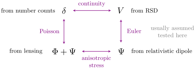
It is interesting to notice that departures from the EEP are, in fact, rarely considered in cosmological tests of gravitation. Notable exceptions are [8, 9], exploiting consistency relations between two- and three-point correlation functions of the matter distribution to test for differences between the way baryons and dark matter fall. In general, however, cosmological tests of gravitation beyond GR do assume that the EEP holds. In an inhomogeneous Universe characterised by scalar perturbations only, there are schematically four degrees of freedom: the matter density contrast , the peculiar velocity potential of the matter flow, and the two Bardeen potentials and (see e.g. [10]). In GR, under reasonable assumptions, is related to by the Poisson equation, to by the continuity equation, and to via Euler’s equation, which closes the system. Alternative theories of gravity generically modify these four relationships.
The standard way to test for deviations from GR in cosmology consists in combining measurements of redshift-space distortions (RSD) with gravitational lensing (e.g. [11]). RSD are indeed sensitive to a combination of and , which can be disentangled by measuring both the monopole and quadrupole of the correlation function, whereas gravitational lensing measures the sum of the two metric potentials . Therefore, these three measurements allow us to test three of the four relationships between and , see fig. 1.
The most common approach consists in keeping the continuity and Euler’s equations unchanged111Here it is implicit that the laws of optics in curved space-time are also left unchanged with respect to GR, so that the whole interpretation of cosmological observations does not need to be modified. and to test for modifications in the Poisson equation and in the relation between and [12, 13]. This has led to precise constraints of the growth rate of structure (see e.g. [14]) and of the anisotropic stress [15, 16]. Relaxing the assumption that Euler’s equation holds opens the cosmic Pandora’s box, adding a freedom which cannot be constrained by the standard cosmological probes. Indeed, if Euler’s equation is allowed to change, then one is left with three probes for four relations. A possible solution is to parameterise modifications to Euler’s equation and Einstein’s equations with free parameters (usually functions of time) and then use redshift-space distortions and gravitational lensing to constrain these parameters. This method is at the core of the effective field theory of dark energy. However, the fact that we have only three observational probes automatically introduces strong degeneracies between the parameters. This degeneracy cannot be broken without adding extra information about the underlying theory of gravity (like for example assuming a specific form for the Lagrangian).
In this article, we show that the so-called relativistic effects in galaxy surveys are the ideal laboratory to test the EEP directly. As such, they can break the degeneracy of the standard set of cosmological probes, induced by potential violations of Euler’s equation. Specifically, as originally shown by [17], some relativistic corrections to the observed galaxy number counts generate a dipole in the two-point correlation function. The amplitude of this dipole is affected by gravitational redshift, i.e. by the gradient of (the time component of the metric). Combining the dipole with RSD allows us therefore to test directly the relationship between and as shown in fig. 1. This would provide the first direct test of the EEP on cosmological scales, since it is sensitive to differences in the way photons and dark matter move222As explained in more detail in sec. 2, we assume here that galaxies follow the motion of dark matter halos, i.e. that there is no velocity bias.. More precisely, we will see that the relativistic dipole contains terms of the form , which exactly cancel if the EEP is satisfied, and do not in general. This shows that even though relativistic effects are not significant enough to improve the constraints on parameters that can be measured via standard RSD and lensing techniques (as pointed out in [18]), they are essential to test for deviations from Euler’s equation that would remain unconstrained without them.
The remainder of the article is organised as follows. In sec. 2, we discuss the notion of free fall in GR and alternative theories of gravity. From the analysis of scalar-tensor and vector-tensor theories, we deduce a quite general parametrisation of the deviations from Euler’s equation in cosmology, at sub-Hubble scales. Then, in sec. 3, we present the relativistic effects in galaxy surveys which give rise to a dipole in the correlation function. We discuss the origin of this dipole, and emphasise its usefulness to constrain the EEP, before explaining how to extract it from the data in practice. In sec. 4, we present Fisher-matrix forecasts on deviations from Euler’s equation in future surveys like DESI and the SKA. Finally, we conclude in sec. 5.
2 Free fall in relativity and beyond
2.1 Generalities
The curious fact that all things seem to fall the same way has been fundamental in the genesis of Einstein’s theory of general relativity (GR) [19]. During the last century, local tests of the weak equivalence principle have reached an exquisite precision [20]; lately, the first results of the MICROSCOPE mission [21] have constrained Eötvös ratio at the level of [22]. Nevertheless, for obvious reasons, the validity of the equivalence principle is more uncertain on astrophysical and cosmological scales, or when the unknown dark matter is concerned.
In cosmology, if we only consider scalar perturbations of a spatially Euclidean Friedmann-Lemaître-Robertson-Walker (FLRW) model in the Poisson gauge, the metric reads
| (2.1) |
where is the scale factor of the background FLRW model, and being respectively conformal time and spatial comoving coordinates, while and are the gauge-invariant Bardeen potentials. If matter is assumed to be freely falling within that space-time, then its flow is characterised by Euler’s equation,
| (2.2) |
where is the peculiar matter velocity field, such that the matter four-velocity reads , is the conformal Hubble rate, and a prime denotes a derivative with respect to conformal time . Equation (2.2) directly follows from the geodesic equation, assuming that . There are, of course, standard corrections to eq. (2.2), due to the fact that fluid elements are not exactly in free fall. The most common deviation comes from the velocity dispersion of the fluid, which gives rise to a pressure term; other forms of stress can yield different corrections, like shear viscosity, turning Euler’s equation into the Navier-Stokes equation. These effects have been considered in a cosmological context, e.g. in [23], and typically manifest on scales below . In this article, we will consider much larger scales and neglect such departures from free fall.
It is also worth mentioning that, even in GR, free fall does not necessarily implies geodesic motion, on which eq. (2.2) is based. Indeed, this implication is valid for test particles, but not exactly for extended self-gravitating bodies, despite the validity of the strong equivalence principle. A first example is the case of spinning objects, whose motion is described by the Mathisson-Papapetrou-Dixon equations [24, 25, 26]. In weak fields, the deviation from geodesic motion is encoded in a force arising from the coupling between the angular momentum of the object and the gravito-magnetic field as [27]. In cosmology, one has at most [28], so that the ratio between and the ‘Newtonian’ force is of the order of , where is the perturbation mode at hand, while are the size and angular velocity of the galaxy. Another known effect, which can make extended objects deviate from geodesic motion, is the so-called self-force, related to the gravitational radiation emitted by the objects [29].
The ‘post-geodesic motion’ phenomenology gets infinitely richer as one allows for theories of gravity beyond GR. Adding new degrees of freedom to gravitation, or new interactions to the dark-universe sector, generically yields violations of the equivalence principles, affecting de facto the way things fall. Such violations can be classified into three categories:
-
1.
Violation of the weak equivalence principle. The universality of free fall is automatically broken if gravity contains degrees of freedom that couple differently to various matter species. Different couplings can be either fundamental [30] or the result of screening mechanisms [31, 32, 33]. This manifests in the apparition of a fifth force, which cannot be absorbed by a simple redefinition of metric (Einstein to Jordan frame). The archetype of this situation is a scalar-tensor theory where the scalar degree of freedom couples differently to dark matter and to the standard model. We will focus on this in sec. 2.2. Another possibility is the direct coupling between dark and baryonic matter [34].
-
2.
Violation of local Lorentz invariance. It is expected, in particular, that the existence of preferred frames or directions implies that objects with different velocities fall differently. An example often cited in this context is the Einstein-æther theory (see sec. 2.3), which contains an additional vector degree of freedom compared to GR. This field can be thought of as the four-velocity of an æther, defining a preferred frame.
-
3.
Violation of the strong equivalence principle. The strong equivalence principle is very specific to GR. Apart from Nordstrøm’s theory [35], none of the alternative seems to satisfy it. Its violation can manifest as a difference between the inertial mass and the passive gravitational mass of a self-gravitating body, depending on its gravitational binding energy . This phenomenon is known as the Nordvedt effect [36], and is quantified by the parameter , as . For a galaxy, , so that this effect is very small even if . Tests of the strong equivalence principle using black holes have been proposed recently in [37, 38].
We restrict our analysis to models where the particles of the standard model (in particular photons) are minimally coupled to gravity, so that the EEP applies to this matter sector, in agreement with experiments. Only dark matter will be allowed to couple non-minimally to the additional gravitational degrees of freedom. Yet, we will assume that the motion of dark matter is directly traced by the motion of galaxies; in other words, there is no velocity bias, . This assumption could seem to be at odds with the fact that we are precisely looking for deviations from the equivalence principle. However, since a galaxy always sits inside a dark matter halo, the latter exerts a binding force on the former, which is very likely to dominate any difference in the way baryonic and dark matter experience gravitation. Such a difference would simply lead to a shift between the baryonic and dark-matter centres of mass [39], which has been used in [40] to constrain the existence of a fifth force in the local Universe. As such, the method proposed in the present article to test the EEP is not based on the difference between the motion of dark matter and baryons, contrary to [9]. It is instead based on the difference between the motion of dark matter and photons.
Based on these considerations, we parameterise modifications from Euler’s equation (2.2) in the following way
| (2.3) |
Here and are two free functions of time that encode modifications in the way dark matter (and consequently galaxies) fall in the gravitational potential . The aim of this paper is to constrain these free functions using relativistic effects. Equation (2.3) is quite general and contains a rich phenomenology. The parameter encodes the effect of a fifth force acting on dark matter. The parameter can be thought of as a friction term, which modifies the way the velocity redshifts away. As we will see, the specificity of relativistic effects is that they can constrain and independently of the underlying theory of gravity which generates these modifications.
Before forecasting the constraints on and that we expect from future surveys, let us briefly present two cases which exist in the literature and which generate precisely the kind of deviations written in eq. (2.3).
2.2 Scalar-tensor theories
We first focus on a popular class of alternative theories of gravity/dark energy, namely scalar-tensor theories. We start with a simple example (sec. 2.2.1) in order to get an intuition of how the presence of a scalar degree of freedom affects free fall. Despite its simplicity, this example will turn out to essentially contain the physics of the general case (sec. 2.2.2).
2.2.1 A simple example
Let us consider the simple case of a scalar field , mediating a fifth force via conformal coupling to dark matter only. The corresponding action is
| (2.4) |
where denotes the space-time metric; are respectively the Einstein-Hilbert action and the action of the standard model of particle physics; is the canonical action of a scalar field with a potential ; and finally is the action of dark matter, which is coupled to the metric via a conformal factor . We model dark matter as a set of spin-less point particles, with individual action
| (2.5) |
if denotes proper time with respect to the physical metric , and is the bare mass of the dark matter particle.
For this model, the equations of motions for , , and dark matter are
| (2.6) | ||||
| (2.7) | ||||
| (2.8) | ||||
| (2.9) |
Let us comment on the notation. We chose to call the stress-energy tensor of (cold) dark matter in the absence of conformal coupling, and ; must be thought of as related to the number of dark matter particles, while is the four-velocity of the dark matter flow. Note that is conserved, by virtue of eq. (2.8).
The presence of the conformal coupling between dark matter and has three physical effects:
-
1.
It changes the dark matter active gravitational mass by a factor , as this factor multiplies the bare stress-energy tensor in eq. (2.6).
-
2.
It also changes its passive gravitational mass and inertial mass by a factor —which is assumed to be positive here— as seen in the left-hand side of eq. (2.9).
-
3.
It adds a fifth force proportional to the gradient of the scalar field333 Expanding the left-hand side of eq. (2.9), one can rewrite it as where is the spatial gradient of in the dark matter frame. This alternative expression has the advantage to show that the effect of the fifth force is frame dependent. Suppose that there exists a frame in which is homogeneous (but not static). If a dark matter particle is at rest with respect to this homogeneity frame, then it experiences no fifth force, since . However, if the particle has a small velocity with respect to that frame, then the spatial gradient becomes , that is a friction force.. This gradient, in turn, is sourced by dark matter via in eq. (2.7). Note that, contrary to gravitation, the fifth force is weaker if it is generated by a hotter dark matter fluid.
In cosmology, if we write , where is the background value of the scalar field, the dark matter equation of motion (2.9) becomes
| (2.10) |
One can then use the other field equations to establish a relationship between and . In the quasi-static approximation, and assuming that dark matter dominates as a source of gravitation, one finds . The modified Euler equation then indeed takes the same form as eq. (2.3),
| (2.11) |
2.2.2 General case: Horndeski theories
In the most general formulation of scalar-tensor theories, the scalar field can also be non-minimally coupled to space-time geometry, generating the broad class of Horndeski theories [41, 42] and beyond [43, 44, 45]. Besides, every matter species can be in principle conformally and disformally coupled to gravitation. The cosmological behaviour of such theories is conveniently described within the effective-field theory (EFT) approach [46, 47], where the coupling between and gravity is characterised by four (Horndeski) or five (beyond Horndeski) functions of time444The large freedom a priori allowed within this class of models has been significantly reduced with the recent detection of gravitational waves with an optical countrepart [48, 49, 50], with strong implications for cosmology [51, 52, 53, 54, 55, 56, 57], while the coupling between and any matter species is given by two additional functions. Here we follow [47], assuming that baryonic matter is universally coupled to gravity, so that one can choose to work in the associated Jordan frame. Only dark matter is then directly coupled to , conformally and disformally.
In this context, the modified Euler’s equation is found to be [47]555Our notation for is inverted compared to [47], see eq. (2.1).
| (2.12) |
which is identical to eq. (2.10), except that is now replaced by , where fully encodes the coupling between and dark matter. Reducing the analysis to the class of Horndeski theories, one can then perform a similar operation as in sec. 2.2.1, and express as a function of . In the quasi-static limit, and assuming that the energy density of dark matter completely dominates the energy density of baryons, we find
| (2.13) |
where , while is related to the coupling functions of the gravitational sector; see sec. 4 of [47] for further details. Calling , we recover the phenomenological form (2.3) of the modified Euler’s equation.
2.3 Vector-tensor theories
As a further step towards generality, this section deals with a class of vector-tensor theories, namely Einstein-æther theories, with direct coupling between dark matter and æther. We are going to show that, under some reasonable assumptions, the modified Euler equation takes the same form as in eq. (2.3).
2.3.1 Fundamentals
The most natural way to break Lorentz invariance in gravitation, while keeping general covariance, consists in exhuming the idea of an æther, defining a preferred frame. This idea is implemented by equipping gravity with an extra vector degree of freedom , which must be thought of as the four-velocity of æther. Following refs. [58, 59], we consider the action
| (2.14) |
which contains the usual Einstein-Hilbert term, but also the kinetic term for , with
| (2.15) |
the coefficients being free parameters of the theory666We use the same convention as refs. [20, 60]. Note the difference with refs. [58, 61], where mostly-minus signature was used, and . The authors of [62] chose to parameterise the Einstein-æther theory by , with , and .. These parameters are already severely constrained by experiments. On the one hand, tests in the Solar system impose and , where those PPN parameters are given by the combinations [20]
| (2.16) | ||||
| (2.17) |
On the other hand, the recent constraints on the relative velocity of light and gravitational waves set by GW170817 [48] and GRB170817A [48, 49, 50] impose [56], where
| (2.18) |
In the following, we will consider , which can be satisfied by setting if ; see however [63] for a thorough status of the current constraints on the , including constraints from the big-bang nucleosynthesis [62]. The last term in (2.14) is a constraint which ensures the normalisation of the æther four-velocity, while is a Lagrange multiplier. This theory can be considered a low-energy limit of Hořava gravity [64, 65, 66]. Note finally that the action (2.14) can be further generalised [67, 68] by replacing the kinetic term by a general function of .
An explicit violation of the equivalence principle can then be implemented by coupling dark matter particles to similarly to how charged particles couple to the electromagnetic four-potential; namely, the action of a dark matter point particle is taken to be [61]
| (2.19) |
where is the relative Lorentz factor between dark matter and æther, and is a function such that . Due to its similarity with the conformal coupling to a scalar field given in sec. 2.2.1, we expect similar phenomena to appear: fifth force, modification of the inertial and gravitational masses, etc.
The full set of equations of motion for , and dark matter is rather heavy. We choose to leave it in the appendix A, while focussing on the dynamics of dark matter for now. If denotes the four-velocity of the dark matter flow, and its energy density in the absence of coupling to æther, then
| (2.20) | ||||
| (2.21) |
where , and . As in the scalar-tensor case, eq. (2.20) tells us that the bare energy of dark matter is conserved. The phenomenology of eq. (2.21) is richer. On the one hand, the inertial mass is modified by a factor . On the other hand, it experiences two kinds of additional forces. The second term on the right-hand side is a kind of friction, proportional to the relative acceleration between dark matter and æther. The first term is reminiscent of the Lorentz force, being analogous to the field strength of electrodynamics. A more kinetic interpretation consists in viewing like an inertial force, containing both dragging-like and Coriolis-like effects. This rich phenomenology will turn out to highly simplify in the context of linear cosmological perturbations.
2.3.2 Cosmological aspects
In strictly homogeneous and isotropic cosmology, æther has to be comoving with matter in order to preserve the symmetries of the FLRW space-time. Thus and everything goes as if dark matter and æther were uncoupled. The expansion dynamics is nonetheless affected, due to the stress-energy of æther itself. This stress-energy tensor turns out to be directly related to the extrinsic curvature of the homogeneity hypersurfaces, and the net effect is to multiply both and in the Friedmann equations777The effect of æther on the dynamics of cosmic expansion was first considered in [62], for and no cosmological constant. The authors chose to interpret the factor as a renormalisation of Newton’s constant and spatial curvature. Had they considered , they would have concluded that the cosmological constant had to be renormalised as well. by .
At the level of perturbations, things are more involved. Restricting to scalar modes as we did in sec. 2.2, the modified Euler equation of dark matter reads
| (2.22) |
where is the velocity potential associated to , and where we used the notation of [61], , for the effective coupling constant between dark matter and æther. The first constraints on were performed in [60], who obtained by combining CMB and BAO data. More recently, a method based on galactic dynamics was proposed in [69]. Note that, as represents the 4-acceleration potential of dark matter, eq. (2.22) can be written as , where we see that the fifth force is related to the relative acceleration of the two flows.
When the above is combined with the dynamics of æther and gravitation (see appendix A), it can be shown that, in Fourier space, , with
| (2.23) |
and where we introduced , corresponding to the uncoupled dark matter density today, . We can then substitute in the relative acceleration of the two fluids, , and we obtain
| (2.24) |
which has the same form as eq. (2.3), except that the functions encoding departures from Euler are now scale dependent (through ). However, for sub-Hubble modes , , and we are left with
| (2.25) |
up to second order in .
2.4 Discussion
The two theoretical cases investigated in secs. 2.2 and 2.3 produce precisely the kind of deviations proposed in eq. (2.3). One could then wonder how general such a parametrisation is. After all, the fact that we only consider linear scalar perturbations should restrict the possible modifications of Euler’s equation. An apparently reasonable guess for the latter would be , where represents the extra degrees of freedom ( in the scalar-tensor case, in the Einstein-æther case, etc.) and where is linear with respect to its arguments. One would then use the other equations of motion to eliminate , so that , which strongly resembles (2.3).
One could, however, imagine extensions of this parametrisation. First of all, could in principle depend on the time derivative of its arguments. Even in the quasi-static approximation, it is not obvious that all those derivatives could be neglected, in particular if they are combined with spatial derivatives. This leads to the second point, which is that the coefficients and in could not only be time-dependent, but also generically scale-dependent. In our forecasts we will not consider this possibility, but it could lead to stronger constraints by modifying not only the amplitude of the relativistic correlation function, but also its shape.
Finally, let us note that if , then essentially coincides with the Eötvös ratio between dark and baryonic matter. It is automatically the case in the Einstein-æther model, since . In the general scalar-tensor scenario described by EFT, one has
| (2.26) |
which is small if evolves very slowly, but could in principle be of order unity. Physically speaking, it corresponds to the situation where the effect of the running of the dark matter mass is smaller than the effect of the fifth force.
3 Testing Euler’s equation with galaxy surveys
In the previous section, we motivated the general parametrisation (2.3) of deviations of the dark matter flow with respect to Euler’s equation. This section deals with the measurability of such deviations. We will now explain how such a signal can be extracted from relativistic effects in galaxy surveys.
3.1 What galaxy surveys really measure
Galaxy surveys attempt to trace the distribution of matter in the Universe from the number density of galaxies. The main observable is therefore the number of galaxies per unit of observed volume, i.e. per pixel of the sky (subtended by a solid angle ) and per redshift bin (see fig. 2). The inhomogeneity of the distribution of galaxies is then quantified by
| (3.1) |
where is the average of over all the pixels, i.e. the total number of observed galaxies divided by the volume of the survey.
The observable does not only contain information about the matter density contrast around the point , but also about the relation between the observed pixel and the corresponding physical volume. Indeed, the gravitational effects of matter inhomogeneities affect the propagation of light, and its frequency. As a consequence, a given pixel can be first physically larger or smaller compared to its counterpart in a strictly homogeneous Universe, and second it can be physically closer or further away from the observer than it would be in a homogeneous Universe. These contributions to have been calculated in [70, 71, 72] at linear order in scalar cosmological perturbations. The result is conveniently written as
| (3.2) |
where is the standard expression of , used in all galaxy surveys, and which already accounts for the effect of biased tracers and redshift-space distortions; contains the so-called relativistic effects, which are corrections to the redshift (Doppler and Einstein effects, integrated Sachs-Wolfe effect, …), and hence ensure the correct estimation of the physical depth and width of redshift bins; and finally denotes the contribution of gravitational lensing, which translates the observed angular size of a pixel into physical areas. Their expressions are
| (3.3) | ||||
| (3.4) | ||||
| (3.5) |
Here denotes the linear bias of the matter tracer (typically galaxies), and is the comoving radial coordinate in the direction of ; in eq. (3.4) and (3.5), denotes the slope of the luminosity function which parameterises the magnification bias and is the transverse Laplacian. Note that, in eq. (3.4), we dropped the terms of involving the gravitational potentials and without spatial derivatives, because their contribution to the dipole presented in the next subsection is suppressed by with respect to the other terms.
Let us further focus on the relativistic correction given by eq. (3.4). The first term denotes de contribution from gravitational redshift, while the other terms are Doppler effects. The fact that gravitational redshift depends directly on allows us to test Euler’s equation in a model-independent way. We notice that three of its terms exactly cancel if Euler’s equation is satisfied. This turns out to be a direct consequence of Einstein’s equivalence principle—we refer the interested reader to appendix B for more details about this connection. Thus, relativistic effect in galaxy surveys are an ideal laboratory to look for violation of the equivalence principle. If Euler’s equation is violated according to our proposition (2.3), then eq. (3.4) becomes
| (3.6) |
where a couple of terms vanish for . In the remainder of this section, we show how to extract from galaxy surveys.
3.2 Dipolar correlations
The simplest way of extracting cosmological information from galaxy surveys consists in using the two-point correlation function of ,
| (3.7) |
Due to statistical homogeneity and isotropy, only three out of the six variables are necessary to parameterise , because only the relative position of the two pixels matters. A convenient parametrisation, depicted in fig. 3, consists in locating, for example, pixel 2 relatively to pixel 1 by their mutual distance and the angle between the axis and the mean line-of-sight . We thus write , where is the redshift of the pixel .
A key advantage of this parametrisation is that the various contributions to depend differently on the angle . For example, it is well known that redshift-space distortions yield a quadrupole and hexadecapole in terms of [73, 74]. It turns out that relativistic effects add a dipole and an octupole to this picture [17, 75], which makes them identifiable in the data888Note that in the power spectrum, relativistic effects are identifiable by the fact that they generate an imaginary part [76, 77].. Let us briefly summarise why such a dipolar structure appears (see [17, 75] for more detail).
As an example, we focus on the correlation between the first term in eq. (3.3) (density) and the first term of eq. (3.4) (gravitational redshift),
| (3.8) |
Each of these terms is antisymmetric with respect to the exchange of , which means that they have a dipolar component in terms of the angle depicted in fig. 3. Indeed, suppose that there is an over-density at []. This generates a potential well around , with directed outwards. Thus, if is located behind along the line of sight (), then ; conversely, if is located between and the observer (), then . The same reasoning applies if there is an under-density at .
This antisymmetry of gravitational redshifts can be understood as in fig. 4 (see also fig. 2 of [17]). Consider two redshift bins located respectively in front of, and behind, an over-density. The closer a galaxy is to the over-density, the stronger its gravitational redshift. This distorts the iso- surfaces in real space, as gravitational redshift mimics the effect of cosmic expansion: the stronger the gravitational field experienced by a galaxy is, the less far from the observer it needs to be in order to have a given redshift. Hence, the physical thickness of the bin in front of the over-density is effectively squeezed, so it potentially contains less galaxies, which reduces , and conversely for the bin located behind the over-density, whence the dipole. The same kind of reasoning can be made for the effect of velocity and acceleration.
In eq. (3.8), is accompanied with . It is then not hard to see that the dipoles associated to each term exactly compensate, because exchanging and corresponds to changing into . However, this cancellation does not happen if one takes the cross-correlation between two types of tracers, with different biases. For instance, correlating bright (B) and faint (F) galaxies with respective biases , eq. (3.8) becomes
| (3.9) |
Both terms still contain opposite dipoles, but the former is proportional to , while the latter is proportional to . There is, therefore, a net dipole in proportional to .
3.3 Extracting the dipole
Because the standard contributions to the cross-correlation function do not contain any dipolar component in the flat-sky approximation, relativistic effects can be extracted by integrating the latter with a suitable antisymmetric kernel. This subsection summarises the construction of an estimator of the dipole (see [78] for more detail).
3.3.1 Set-up and conventions
To calculate the multipoles of the correlation function, we write in Fourier space, for which we use the convention999 is measured as a function of , but it can now be re-written in terms of conformal time , since the error that is made when one goes from to using the background relationship has been consistently included in our derivation of . In the following, we will use indistinctly or .
| (3.10) |
We define the velocity potential in Fourier space through , so that has the same dimensions as , i.e. [length]3. Note that is then related to the Fourier transform of by a factor . We assume that the continuity equation is valid, as discussed in sec. 2. For sub-Hubble modes (),
| (3.11) |
This allows us to write as a function of only, in particular
| (3.12) | ||||
| (3.13) |
where
| (3.14) |
encodes the deviations from Euler’s equation. Here we have assumed that the growth of density perturbation, , defined through is scale-independent. This is true in the quasi-static limit of the models described in sec. 2. In general, deviations from GR can introduce a scale-dependence in , but we will not consider this possibility in the following. The growth rate , defined through
| (3.15) |
is therefore scale-independent as well, and so is defined in (3.14).
3.3.2 Expression of the cross-correlation function
In the cross-correlation of two populations of galaxies, bright B and faint F, the only quantities which depend on the galaxy population in eqs. (3.12) and (3.13) are the biases and and the slopes and . Following [17] we can write, in the flat-sky limit,
| (3.16) |
where denotes the mean redshift of the survey (or of the redshift bin of interest), and we remind the reader that is the separation between the galaxies, while denotes the orientation of the pair of galaxies with respect to the mean direction of observation .
In eq. (3.16), is the standard correlation function containing a monopole, quadrupole and hexadecapole in [74, 73]. The relativistic contribution is given by
| (3.17) |
where denotes the Legendre polynomial of degree , and
| (3.18) |
Here is the matter power spectrum today, , while denotes the spherical Bessel function of degree . The relativistic correlation comes from the correlation between the standard term (3.3) and the relativistic term (3.4) and, as anticipated in sec. 3.2, it is completely anti-symmetric, because it consists of a dipole and an octupole in . The correlation of the relativistic contribution with itself also contributes to , but we neglect it here, because it only consists of a monopole and a quadrupole, eliminated in the dipole extraction performed in the next paragraph.
The third contribution to eq. (3.16), , represents the wide-angle corrections to the flat-sky correlation function. As discussed in refs. [17, 78] the wide-angle corrections from density and redshift-space distortions also generate a dipole and an octupole in the correlation function. As such, they contaminate the measurement of the relativistic contribution. The wide-angle effects are minimised by using the angle to extract the dipole, i.e. the angle between the direction of the median of the pair and the direction of observation—see [78, 79] for a detailed discussion about other possible angles. This contribution is given by
| (3.19) |
with
| (3.20) |
Comparing eq. (3.19) with eq. (3.17), we see that is suppressed by with respect to . However is enhanced by a factor with respect to . Since these two effects compensate and the wide-angle correction becomes of the same order of magnitude as the relativistic contribution (see also fig. 8 of [17]).
The fourth term in eq. (3.16), , denotes the evolution corrections. These are due to the fact that the biases, growth rate, and slopes of the luminosity function evolve with redshift, and consequently also gives rise to a dipole and octupole. However, as shown in fig. 11 of [17], these evolution corrections are always sub-dominant with respect to both the relativistic contribution and the wide-angle corrections. We can therefore safely neglect them.
3.3.3 Estimator of the dipole
From eqs. (3.16) and (3.17) we see that the optimal way to test Euler’s equation is to extract the dipolar modulation in the two-point correlation function. First, this allows us to completely get rid of the standard correlation function (which is insensitive to the parameters and that we want to constrain). And second, it strongly reduces the impact of the evolution and lensing contributions which are negligible in the dipole. Hence the only two relevant contributions to the dipole are the wide-angle contribution and the relativistic contribution. As shown in eq. (3.19) the wide-angle contribution is insensitive to the parameters and . As such this contribution is a contamination that we would like to remove. As discussed in [17], this can be done observationally by removing the quadrupole of the bright and faint populations from the dipole, i.e. by constructing the following estimator
| (3.21) | ||||
where denotes the volume of the survey (or of the redshift bin of interest), is the length of the cubic pixel in which is measured, the sum runs over all pairs of pixels in the survey and is the Kronecker delta function. The first line in (3.21) isolates the dipole contribution in the cross-correlation between bright and faint galaxies (the minus sign ensures that the correlation does not vanish under the exchange of bright and faint galaxies). The second line removes the wide-angle effect. Taking the mean of the estimator and going to the continuous limit101010The continuous limit is obtained by replacing the sum over pixels by a 3-dimensional integral and the Kronecker delta function by a Dirac delta function . we find indeed
| (3.22) |
with . Note that eq. (3.22) is valid in the linear regime. An equivalent estimator has been constructed fo measure gravitational redshift in clusters [80, 81] and in the non-linear regime of large-scale structure [82]. The modelling and interpretation of the signal in the non-linear regime is however much more complicated [83, 84, 85] and its use to test Euler’s equation is not straightforward.
4 Forecasts: are deviations from Euler detectable?
We now forecast the detectability of deviations from Euler’s equation in future surveys. We consider first the SKA survey and then the DESI survey.
4.1 Constraints from the SKA
In its second phase of operation, the SKA will observe galaxies over 30’000 square degrees, from redshift 0.1 to redshift 2. We split the redshift range into bins of width and use the number densities derived in table 3 of [86]. In each redshift bin, we calculate the signal from eq. (3.22) and the covariance matrix . The covariance matrix has been calculated in [78, 87]. In general, covariance matrices contain a shot noise contribution, a cosmic variance contribution and a mixed contribution. However, as shown in [78, 87], the dipole estimator automatically removes the cosmic variance contribution from density and redshift-space distortions. Fitting for a dipole in the data allows us therefore not only to get rid of the dominant standard contribution (density and redshift-space distortion) in the signal but also in the noise. As such, the dipole estimator is a powerful tool to isolate the relativistic contributions. The expression for the covariance can be found in appendix C. Note that subtracting the wide-angle effects adds an additional contribution to the covariance. However, as shown in [87], this contribution is always strongly subdominant with respect to the shot noise and mixed contribution (see fig. 2 of [87]).
We split the population of galaxies into a bright and a faint population with the same number of galaxies. We use the mean redshift given in table 3 of [86] and we assume that the two populations are equally distributed around this mean redshift, with a redshift difference . The signal-to-noise is directly proportional to the bias difference. As an example, in BOSS, a bias difference of 1 has been measured between the bright and faint populations of luminous red galaxies (LRG’s) [88]. In the main galaxy sample of SDSS, galaxies have been split into six populations according to their luminosity, with a bias ranging from 0.96 to 2.16 [89, 90]. For the HI galaxies targeted by the SKA, the expected bias difference is less well known, but a difference of 0.5 seems quite conservative. As we will see in sec. 4.1.2 the constraints on deviations in Euler’s equation scale directly with the bias difference. The signal-to-noise and the constraints depend also on the slope of the luminosity function and . We fix those to be zero. We assume a background cosmology consistent with CDM, with the fiducial cosmological parameters from BOSS DR11 [91]: and .
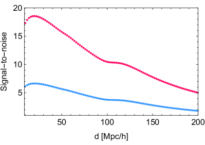
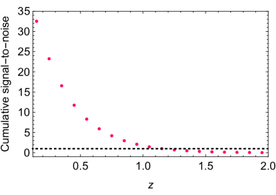
In fig. 5 we plot the signal-to-noise of the dipole. In the left panel, we show the signal-to-noise at each separation , in the lowest redshift bin (red dots) and in the bin (blue dots). We use a pixel size . We see that the signal-to-noise peaks around . In the right panel we show the cumulative signal-to-noise from , as a function of redshift. Above the cumulative signal-to-noise drops below 1, meaning that the dipole is not observable. The cumulative signal-to-noise over the whole range of separation and redshift is of 46.4, showing that the dipole will be robustly measured with the SKA.
4.1.1 Constraints from the dipole
We first forecast the constraints on and that we would obtain using only the dipole estimator defined in eq. (3.21). We fix all cosmological parameters and the biases to their fiducial value. Cosmological parameters are indeed well measured by the CMB. The biases on the other hand are unconstrained by the CMB, but as we will see in sec. 4.1.2 they can be robustly constrained by the standard multipoles. For and we assume that they evolve according to
| (4.1) |
where , and similarly for . As discussed in [92] this evolution ensures that the deviations vanish when the background dark energy density is negligible, like at high redshift, and one recovers Euler’s equation. We use fiducial values .
As a first example we assume that and are the only deviations from general relativity, in particular we assume that the growth function evolves as in a CDM Universe. In the scalar-tensor and vector-tensor models described in sec. 2 deviations from Euler’s equations are usually accompanied by deviations in the growth rate. However one could imagine other models where this is not the case, and the only deviations from general relativity would be in Euler’s equation.
We construct the Fisher matrix for and
| (4.2) |
where , and denotes the covariance matrix of the dipole estimator. In (4.2), the sum runs over all pixel’s separations and all redshift bins. We account for correlations between separations (see appendix C), but we neglect correlations between different redshift bins. We use pixel’s size of and pixel’s separations . We choose since we have checked that the constraints do not improve if we include larger separations. For the minimum separation, we use . At this scale the impact of non-linearities on the dipole is of the order of 10 %111111We estimate the impact of non-linearities on the dipole in the following way: we use the linear continuity equation to express the velocity in terms of the density, and then we use halo-fit to compute the non-linear density. This procedure is of course not completely correct since non-linearities modify the continuity equation, but it allows us to estimate the scale at which non-linearities become important.. As we will see below, increasing to , where the impact of non-linearities on the dipole is already less than 2 %, has almost no effect on the constraints on and .
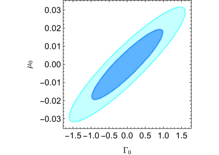
In the left panel of fig. 6 we show the joint constraints on and . There is a strong degeneracy between the two parameters, leading to relatively large marginalised 1- errors of and . This degeneracy can be understood from eq. (3.22). We see that the amplitude of the dipole depends on [first term in the expression (3.14) of ] as well as on individually. However this second dependence is much weaker than the first one at low redshift, since the terms in the second parenthesis are proportional to the second time derivative of the growth factor, . As a consequence and are strongly correlated. However, as discussed in sec. 2.4, in vector-tensor theories, . In the EFT of dark energy is generically not zero, but it is directly proportional to the background evolution of the scalar field. As such it is generically expected to be significantly smaller than . It is therefore natural to explore how the constraints change when . In this case, the constraints on strongly tightens and we obtain .
Comparing with the constraints on standard modified gravity parameters in [93, 94] we see that the constraints on are weaker by 1 to 3 orders of magnitude. This is not surprising since the signal-to-noise of the dipole is weaker than that of the standard multipoles. However, as discussed in the introduction, a constraint on would provide the first direct test of the equivalence principle at cosmological scale, which cannot be probed in a model-independent way with the standard multipoles. In [92], constraints on Euler’s equation are obtained indirectly in the specific case of scalar-tensor theories. In this model, the parameters that modify Euler’s equation also modify the growth of structure, which is measured via the standard multipoles. These constraints are therefore directly related to the specific choice of model: scalar-tensor theories. Constraints of the order of are obtained in this case, varying each parameter individually. Marginalising over all modified gravity parameters degrade the constraints significantly [95]. This shows the complementarity of relativistic effects, which break the degeneracy between parameters and which can directly probe Euler’s equation, without underlying assumptions about the model.
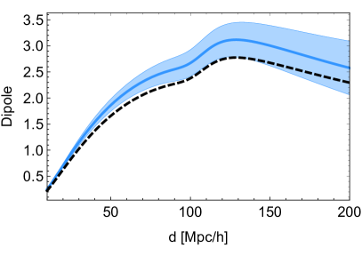
In fig. 7 (left panel) we show the dipole in the lowest redshift bin when (blue solid line) and when (dashed black line). We see that in this case the deviation due to the breaking of the equivalence principle is larger than the error bars (coloured blue region) in the range . Combining all separations and all redshifts allow us to see deviations already for . In the right panel of fig. 7, we show the constraints on in each redshift bin. We see that the constraints come mainly from low redshift.

As discussed above, generic modified gravity models generate not only deviations in Euler’s equation, but also deviations in the way structure are growing as a function of time, i.e. in the growth function . We model this in the following way
| (4.3) |
where denotes the growth function in a CDM universe, and we let the deviation evolve as in eq. (4.1). The growth rate can then be written as a function of
| (4.4) |
where denotes the growth rate in a CDM universe. Inserting (4.3) and (4.4) into eq. (3.22), and linearising in the deviations, we can forecast the constraints on and , fixing .
The joint constraints are shown in the right panel of fig. 6. We see that is less degenerated with than with . This comes from the different time dependence that multiplies these two parameters in eq. (3.22). The marginalised constraints on each of the parameters are given by and . Allowing for the growth rate to vary degrades therefore the constraints on by a factor 2.5.
Finally, let us note that all these constraints are obtained while fixing the bias of the bright and faint populations to their fiducial value. If instead we let the biases vary, we loose all constraining power, since the bias difference in each redshift bin is strongly degenerated with a change in the growth rate and with modifications to Euler’s equation. However, in addition to measuring the dipole of the correlation function, one can also measure the monopole, quadrupole and hexadecapole of the bright and faint populations separately. As we will see in the next section, this allows us to break the degeneracy between the biases, the growth rate and the modification to Euler’s equation .
4.1.2 Constraints from the dipole combined with standard multipoles
We now consider 7 observables: the cross-correlation dipole, and the monopole, quadrupole and hexadecapole of the bright and of the faint populations. In the forecasts, we neglect the covariance between different multipoles. We take however into account the covariance between the monopole of the bright and of the faint population, as well as between their quadrupole and hexadecapole. These covariance matrices have been calculated in [87] and are summarised in appendix C.
As in the previous section, we fix the cosmological parameters to their CDM fiducial value. We consider and as free parameters (as motivated above we fix ). We assume that the bias of the bright and faint population evolves in the following way [86]
| (4.5) | |||||
| (4.6) |
where as before we fix the bias difference . We have therefore four additional free parameters and that we want to constrain. We choose their fiducial value as in [86] (see table 6): and . In this way the bias of the bright and of the faint population are uncorrelated, but their difference is always of 0.5. As shown below, the constraints can easily be rescaled according to the bias difference.

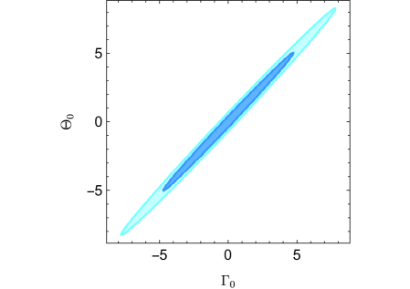
In fig. 8 we show the joint constraints on and marginalised over the four bias parameters. We see that adding the standard multipoles strongly tightens the constraints on : the marginalised error on becomes , consistent with [46]. This is not surprising since the monopole, quadrupole and hexadecapole provide three different combinations of and of the bias, which can then be both robustly constrained. Since the signal-to-noise of the even multipoles is significantly larger than that of the dipole, we find that adding the dipole in the forecasts does not improve the constraints on at all. This is consistent with the conclusion of [18] which showed (using the angular power spectrum ) that relativistic effects do not improve the constraints on parameters that govern the growth of structure, like (see however [96] for specific cases, where this may not be true). The usefulness of relativistic effects is therefore to test for deviations that cannot be probed with standard observables, like deviations in the equivalence principle. The marginalised error on is also tightened by the combined analysis: . Hence even though the standard multipoles are not sensitive to , they improve the constraints on by breaking the degeneracy with . Comparing with the results in sec. 4.1.1, we see that we recover the constraints that we had on from the dipole when all other parameters were kept fixed. Combining the dipole alone with the standard multipoles of the bright and faint populations provides therefore an ideal way of testing for deviations in both the growth of structure and in Euler’s equation .
Note that in these forecasts we have assumed that evolves as in eq. (4.1). If instead we choose a constant over the whole redshift range (in the model of [46], this would correspond to a fixed coupling of the dark matter to the scalar field), then the constraints on tightens to . This comes from the fact that in this case high redshift bins contribute more to the constraints since does not decrease with redshift.
For these forecasts we have used as minimum separation . Increasing this to , in order to reduce the impact of non-linearities, does very slightly degrade the constraint on from to . The constraint on is more sensitive to since it changes from to . This can be understood by the fact that the standard multipoles are more strongly affected by small scales than the dipole. Comparing eq. (3.18) with eq. (3.20) we see indeed that the standard multipoles contain a factor more than the relativistic dipole. As such, at a given separation, the dipole is less sensitive to large ’s than the standard multipoles.
Finally, as discussed before, the forecasts are directly sensitive to the bias difference between the bright and faint population, since the estimator (3.22) is proportional to . Here we have used a fixed difference: . Increasing this bias difference to 1, we find that the constraint on tightens by roughly a factor 2, , while the constraint on remains almost the same, . Equivalently decreasing the bias difference to 0.25 decreases the constraint on by roughly a factor 2, , while the constraint on remains almost the same, . Hence as expected the constraint on scales directly with the bias difference .
4.2 Constraints from DESI
In the previous section we have seen that the SKA will provide meaningful constraints on deviations from the equivalence principle. On a shorter timescale, the DESI survey [2] is expected to map galaxies over a large range of redshifts and scales and could already deliver interesting tests of the equivalence principle. The DESI survey will observe different types of galaxies at different redshifts. At low redshift, , the Bright Galaxy Sample (BGS) is expected to contain approximately 10 million of galaxies. At middle redshift, , DESI will observe Luminous Red Galaxies (LRG) and Emission Line Galaxies (ELG). Finally at high redshift, , only ELG’s will be detected. The area of the survey is expected to reach 14’000 square degrees. For our forecasts, we use the bias evolution given in sec. 3 of [2] and the number densities and volumes given in tables 2.3 and 2.5. We forecast the constraints on , and the biases in each range of redshifts, and we then combine them. As before we neglect the covariance between individual redshift bins.
In the lowest range of redshift, , we split the 10 millions BGS into two equal populations (bright and faint) with a bias difference . We assume that the bias of each population evolves as
| (4.7) | |||||
| (4.8) |
where and are two free parameters with fiducial value [2].
In the middle range of redshift, , we have two populations of galaxies, the LRG’s and the ELG’s, with very different biases. However, the number density of ELG’s is significantly higher than that of LRG’s. Hence it is not optimal to use only cross-correlations between these two populations. We split therefore the galaxies into three populations. Population A contains all the LRG’s with a bias
| (4.9) |
where the fiducial value . Population B contains half of the ELG’s and population C the other half, with biases
| (4.10) | |||||
| (4.11) |
where is fixed and the fiducial values of the free parameters is [2]. With this split we have a similar number of galaxies in each population: 3.9 millions LRG’s, 4.6 millions bright ELG’s and 4.6 millions faint ELG’s. As shown in [78], we can then increase the signal-to-noise of the dipole estimator by weighting each pair of galaxies by the bias difference between the populations. This weighting is optimal in the regime where shot noise dominates. The covariance matrix of this estimator is given in appendix C.
Finally in the high redshift range, , we split the 7.8 millions ELG’s into two equal populations, with the same two free bias parameters and .
| combined | ||||
| 1.9 | ||||
In each case we calculate the cross-correlation dipole, as well as the monopole, quadrupole and hexadecapole of each population, in thin redshift bins of width . We neglect correlations between different multipoles, but we take into account the correlation between the same multipole of different populations. We use the range of separation . We assume that , so we have in total 7 free parameters: and . The marginalised constraints on and are summarised in table 1. We see that the combined constraint on reaches . This is 7 times larger than the constraint expected from the SKA, but it would provide the very first test of the equivalence principle at cosmological scales. Since we have never directly observed dark matter particles fall into a gravitational potential, a value of order unity for is not excluded.
5 Conclusion
In this paper, we have shown that relativistic effects can be used to test the equivalence principle directly. We have used the dipole in the cross-correlation function of bright and faint galaxies to constrain deviations from Euler’s equation. Such deviations would modify the relation between the galaxy velocity and the time component of the metric . They are therefore unconstrained by the monopole, quadrupole and hexadecapole of redshift-space distortions, since these observables are sensitive to the density and velocity, but not to the metric. Adding information from gravitational lensing is not enough, since lensing is affected by the sum of the two metric potentials, , and not by individually. The cross-correlation dipole provides therefore a unique opportunity to test for deviations in Euler’s equation since it is directly sensitive to via the effect of gravitational redshift.
We have found that future surveys like DESI and the SKA can provide meaningful constraints on deviations from Euler’s equation. Comparing with previous forecasts on modifications of gravity, we find that our constraints are weaker by 1-3 orders of magnitude with respect to constraints on the growth rate of structure and on the anisotropic stress. This is due to the fact that the signal-to-noise of the dipole is significantly lower than that of the RSD multipoles and of gravitational lensing, that are used to constrain those deviations. Hence the equivalence principle will always be more difficult to constrain than the growth of structure or the relation between the metric potentials. On the other hand, since we have never observed dark matter directly, any constraint obtained from the dipole would provide a significant improvement in our knowledge of this component.
Finally, let us emphasise that the specificity of our work is to test the equivalence principle in a model-independent way. The parametrisation that we use is motivated by the example of scalar-tensor theories and Einstein-æther theories, but it is in reality completely general. Indeed, at no point in our analysis we need to refer to a specific class of Lagrangian or theory. Our framework allows us to test for any deviation in Euler’s equation, independently of the underlying theory. If on the other hand one chooses to start from a specific Lagrangian, with a set of free functions, then the rules of the game completely change. These free functions would indeed modify in a specific way the growth of structure, the relation between the metric components and Euler’s equation. One can then indirectly test for deviations in Euler’s equation using RSD and lensing, through a measurement of these free functions, as for example in [92]. Such an approach would deliver more stringent constraints, since these free functions are very well measured via the growth rate, but it has the disadvantage that it is related to a specific class of model.
Therefore, the real usefulness of relativistic effect is not to improve the constraints on parameters that can be measured via other methods. As pointed out in [18], relativistic effects are too small to have a measurable impact in this case. The usefulness of relativistic effects is rather to test for deviations that cannot be tested in a model-independent way by other methods. In this sense, relativistic effects are really complementary to standard observables and do add extra information.
Acknowledgements
We thank Filippo Vernizzi, Jérôme Gleyzes, and Sergey Sibiryakov for clarifications about, respectively, scalar-tensor and Einstein-æther theories. We also thank Ruth Durrer and Alex Hall for interesting discussions. We acknowledge support by the Swiss National Science Foundation.
Appendix A The equations of Einstein-æther gravity
In this appendix, we give all the equations of the Einstein-æther gravity that were necessary to derive eq. (2.22). In most of this appendix, we keep full generality for the parameters of the theory. Our equations can be compared with [61], where a comprehensive analysis of the Einstein-æther model with coupling to dark matter was performed.
A.1 Equations of motion
Recall that the action for gravity and æther is
| (A.1) |
with , and being a Lagrange multiplier, while the action of a dark point particle with bare mass is
| (A.2) | ||||
| (A.3) |
where, in eq. (A.2), is the particle’s proper time and is its Lorentz factor in the æther frame; in eq. (A.3), is an arbitrary parameter along the particle’s worldline . This latter form, albeit more complicated, is necessary to identify where actually depend on and .
Dark matter.
There are two ways of deriving the equation of motion for dark matter: either by directly differentiating with respect to , or from a Noether-like calculation, using the invariance of under diffeomorphisms. We choose here the second method as it will also bring energy conservation. Considering that is the superposition of many , such that there are particles per unit volume, then the stress-energy tensor of dark matter is found to read
| (A.4) |
with the symmetrisation convention . In the functional derivative of (A.4) we assumed that is the fundamental æther variable.121212One could make another choice and consider that is the fundamental variable. In this case the result would not contain . This term would then have to come from the æther action. The important thing is to choose a convention and follow it consistently. The equation of motion is then
| (A.5) |
which yields the system given in sec. 2.3,
| (A.6) | ||||
| (A.7) |
with , and a dot is a derivative with respect to proper time.
Aether.
The equation of motion for æther is obtained by directly differentiating the total action with respect to , which yields
| (A.8) |
Defining , and using the constraint , we can eliminate the Lagrange multiplier and get
| (A.9) |
where is the spatial metric in the rest frame of æther.
As for its stress-energy tensor, a long but straightforward calculation, still assuming that is the independent variable, yields
| (A.10) | ||||
| (A.11) | ||||
| (A.12) | ||||
| (A.13) | ||||
| (A.14) | ||||
| (A.15) |
Gravity.
The Einstein field equation is, as usual, obtained by differentiating the total action (with many dark matter particles) with respect to the metric, and simply reads
| (A.16) |
in which one just has to plug the expressions of the stress-energy tensors obtained in the previous paragraphs. The result for the total stress-energy tensor is
| (A.17) |
with . Note that our total stress-energy tensor looks different from eq. (82) of [61]. This is due to our different conventions for the signature of the metric and for the sign of . One can check that, using the equation of motion of æther, and re-introducing the Lagrange multiplier, that our results agree.
A.2 Cosmology
A.2.1 Background
First consider an FLRW space-time. The symmetries of this solution impose that the æther flow reads , where denotes cosmic time. The dynamics of dark matter and æther are thus trivial, and the only degree of freedom is the scale factor. Plugging the solution into Einstein’s equation, one finds the modified Friedmann equations
| (A.18) | ||||
| (A.19) |
where is the spatial curvature of the homogeneity hypersurfaces. We could have added a cosmological constant to the right-hand side by adding the corresponding term in the action.
The apparition of the factor in the “kinetic side” of the Friedmann equations can be understood as follows. Geometrically, are related to the extrinsic curvature of the homogeneity hypersurfaces, with , being the unit normal to the hypersurfaces. Now using the decomposition of the Ricci scalar, we can rewrite the Einstein-æther Lagrangian as
| (A.20) | ||||
| (A.21) | ||||
| (A.22) |
Hence the intrinsic-curvature part is unchanged, but the extrinsic-curvature part is renormalised, whence the result in the Friedmann equations.
A.2.2 Perturbations
We now consider scalar cosmological perturbations about the FLRW background in the Poisson gauge. The metric is taken to be the same as in eq. (2.1), and the four-velocity of æther and dark matter are given, respectively, by and . Their normalisation implies , and we introduce the velocity potentials such that and . As usual, the dark matter density perturbation is parameterised as .
Dark matter.
While the continuity equation for dark matter remains unchanged,
| (A.23) |
with , the modified Euler equation (2.21) reads
| (A.24) |
or if we introduce the four-acceleration potential , and the coupling constant , as stated in the main text.
Aether.
At linear order, the equation of motion (A.9) is shown to read
| (A.25) |
When we take into account the observational constraints , it reduces to
| (A.26) |
Gravity.
Finally, the components , , and the trace-less part of of the Einstein field equation yield respectively
| (A.27) | |||
| (A.28) | |||
| (A.29) |
which, for , becomes
| (A.30) | ||||
| (A.31) | ||||
| (A.32) |
Modified Euler equation.
Let us use the whole set of the above equations to simplify the modified Euler equation. In particular, we would like to rewrite the relative acceleration potential in terms of only. For that purpose, we use the background dynamics, which implies in particular
| (A.33) |
which we inject into eq. (A.31), and then inject the latter into the equation of motion (A.26),
| (A.34) |
In Fourier space, this can be rewritten as , where
| (A.35) |
from which we deduce
| (A.36) |
and the modified Euler equation finally reads
| (A.37) |
For , , and the above reduces to
| (A.38) |
which has the same for as eq. (2.3), with and .
Appendix B Redshift corrections and equivalence principle
This appendix aims at emphasising the fundamental link between the cancellation of some relativistic corrections to the galaxy number counts and the equivalence principle. For that purpose, let us forget about cosmology, and consider the simple case of two light sources in radial free fall onto a massive object, as depicted in fig. 9, and discuss how an observer, at rest far from them, sees the light they emit.
We first work in the observer’s frame. For simplicity, suppose that both sources are initially at rest, separated by a distance . At , the source closest to the massive object, undergoing a gravitational potential emits a photon with frequency in its own frame. This photon reaches the source at time , where we have neglected the velocity of with respect to the speed of light. This velocity, however, is not zero, because falls in the gravitational field of the massive object, with an acceleration , and hence during ’s propagation time, it gained a velocity .
Now suppose that, at , emits a photon with frequency . Then, in principle, this frequency differs from the frequency of in the frame of , because of both Doppler and Einstein effects. Namely, at lowest order,
| (B.1) |
Therefore, everything happens as if the source were sending simultaneously two photons with different frequencies. Whatever happens to those photons, their mutual redshift is preserved until they reach . In an expanding Universe, this reasoning still applies if one replaces by the peculiar acceleration. Once written in comoving coordinates, the corresponding redshift correction reads
| (B.2) |
where we recognise three terms of the six terms of , as written in eq. (3.4).
Of course, since the sources are in radial free fall, , and the two effects contributing to eq. (B.1) cancel exactly. This cancellation must be understood as a consequence of Einstein’s equivalence principle. Indeed, let us consider the above situation in the rest frame of . In that frame, the effects of gravity are eliminated, modulo curvature terms, so appears to be at rest, while light propagates as in Minkowski space-time. Consequently, the frequency of as observed by is unchanged with respect to its emission frequency. The only way to escape this reasoning is to violate the equivalence principle, either by assuming that (i) and fall differently, or (ii) falls differently from and . In this article, we considered possible departures from (ii), where dark matter and photons are not identically coupled to gravitation.
Appendix C Covariance matrices
We need 7 covariance matrices: the covariance of the cross-correlation dipole , the covariance of the monopole (where ), quadrupole and hexadecapole , and the cross-covariance of the bright and faint monopole , quadrupole and hexadecapole . Note that does not denote the covariance of the cross-correlation monopole between bright and faint galaxies, but rather the covariance between the monopole of the bright and the monopole of the faint. The covariance matrix for the monopole is then given by
| (C.1) |
and similarly for the quadrupole and the hexadecapole.
The covariance matrices contain three contributions: a Poisson contribution due to the fact that we observe a finite number of galaxies, a cosmic variance contribution due to the fact that we observe a finite volume and a mixed contribution from Poisson and cosmic variance. Since the standard terms (density and RSD) are always larger than the relativistic terms, we can neglect the contribution from the relativistic terms to the cosmic variance and to the mixed contribution. The only exception is for the covariance of the dipole, where the cosmic variance contribution from the standard terms vanishes. However, the mixed contribution from the standard terms does not vanish and always dominates over the relativistic cosmic variance contribution (see fig. 2 of [87]), so we can safely neglect the latter also in this case. We follow the method developed in [78, 87] to calculate the covariance matrices. We obtain
| (C.2) | ||||
| (C.3) | ||||
| (C.4) | ||||
| (C.5) | ||||
| (C.6) | ||||
| (C.7) | ||||
| (C.8) |
Here denotes the volume of the survey or of the redshift bin of interest, is the number density, and are the fraction of bright and faint galaxies, and is the size of the cubic pixel in which is measured. We use Mpc. The functions and are defined as follows for
| (C.9) | ||||
| (C.10) |
In the forecasts for DESI, we correlate three populations of galaxies A, B and C in the middle redshift range. We optimise the signal-to-noise in this range by weighting each pair of pixels by the bias difference between the populations, as discussed in [78]. The covariance of this new estimator is then given by
| (C.11) | ||||
References
- [1] Planck Collaboration, R. Adam et al., Planck 2015 results. I. Overview of products and scientific results, Astron. Astrophys. 594 (2016) A1, [arXiv:1502.01582].
- [2] DESI Collaboration, A. Aghamousa et al., The DESI Experiment Part I: Science,Targeting, and Survey Design, arXiv:1611.00036.
- [3] EUCLID Collaboration, R. Laureijs et al., Euclid Definition Study Report, arXiv:1110.3193.
- [4] R. Braun, T. Bourke, J. A. Green, E. Keane, and J. Wagg, Advancing Astrophysics with the Square Kilometre Array, PoS AASKA14 (2015) 174.
- [5] LSST Science, LSST Project Collaboration, P. A. Abell et al., LSST Science Book, Version 2.0, arXiv:0912.0201.
- [6] J. Schwinger, On Gauge Invariance and Vacuum Polarization, Physical Review 82 (June, 1951) 664–679.
- [7] S. Liberati, Tests of Lorentz invariance: a 2013 update, Class. Quant. Grav. 30 (2013) 133001, [arXiv:1304.5795].
- [8] A. Kehagias, J. Noreña, H. Perrier, and A. Riotto, Consequences of Symmetries and Consistency Relations in the Large-Scale Structure of the Universe for Non-local bias and Modified Gravity, Nucl. Phys. B883 (2014) 83–106, [arXiv:1311.0786].
- [9] P. Creminelli, J. Gleyzes, L. Hui, M. Simonović, and F. Vernizzi, Single-Field Consistency Relations of Large Scale Structure. Part III: Test of the Equivalence Principle, JCAP 1406 (2014) 009, [arXiv:1312.6074].
- [10] P. Peter and J.-P. Uzan, Primordial Cosmology. Oxford Graduate Texts, 2009.
- [11] A. Ferté, D. Kirk, A. R. Liddle, and J. Zuntz, Testing gravity on cosmological scales with cosmic shear, cosmic microwave background anisotropies, and redshift-space distortions, arXiv:1712.01846.
- [12] L. Amendola, M. Kunz, and D. Sapone, Measuring the dark side (with weak lensing), JCAP 0804 (2008) 013, [arXiv:0704.2421].
- [13] L. Amendola, M. Kunz, M. Motta, I. D. Saltas, and I. Sawicki, Observables and unobservables in dark energy cosmologies, Phys. Rev. D87 (2013), no. 2 023501, [arXiv:1210.0439].
- [14] BOSS Collaboration, S. Alam et al., The clustering of galaxies in the completed SDSS-III Baryon Oscillation Spectroscopic Survey: cosmological analysis of the DR12 galaxy sample, Mon. Not. Roy. Astron. Soc. 470 (2017), no. 3 2617–2652, [arXiv:1607.03155].
- [15] R. Reyes, R. Mandelbaum, U. Seljak, T. Baldauf, J. E. Gunn, L. Lombriser, and R. E. Smith, Confirmation of general relativity on large scales from weak lensing and galaxy velocities, Nature 464 (2010) 256–258, [arXiv:1003.2185].
- [16] Planck Collaboration, P. A. R. Ade et al., Planck 2015 results. XIV. Dark energy and modified gravity, Astron. Astrophys. 594 (2016) A14, [arXiv:1502.01590].
- [17] C. Bonvin, L. Hui, and E. Gaztañaga, Asymmetric galaxy correlation functions, Phys. Rev. D89 (2014), no. 8 083535, [arXiv:1309.1321].
- [18] C. S. Lorenz, D. Alonso, and P. G. Ferreira, Impact of relativistic effects on cosmological parameter estimation, Phys. Rev. D97 (2018), no. 2 023537, [arXiv:1710.02477].
- [19] A. Pais, Subtle Is the Lord… The Science and the Life of Albert Einstein. Oxford University Press, 1982.
- [20] C. M. Will, The Confrontation between General Relativity and Experiment, Living Rev. Rel. 17 (2014) 4, [arXiv:1403.7377].
- [21] https://microscope.cnes.fr/en/MICROSCOPE/index.htm.
- [22] P. Touboul et al., The MICROSCOPE mission: first results of a space test of the Equivalence Principle, arXiv:1712.01176.
- [23] D. Blas, S. Floerchinger, M. Garny, N. Tetradis, and U. A. Wiedemann, Large scale structure from viscous dark matter, JCAP 1511 (2015) 049, [arXiv:1507.06665].
- [24] M. Mathisson, Neue mechanik materieller systemes, Acta Phys. Polon. 6 (1937) 163–2900.
- [25] A. Papapetrou, Spinning test particles in general relativity. 1., Proc. Roy. Soc. Lond. A209 (1951) 248–258.
- [26] W. G. Dixon, Dynamics of extended bodies in general relativity. I. Momentum and angular momentum, Proc. Roy. Soc. Lond. A314 (1970) 499–527.
- [27] C. Chicone, B. Mashhoon, and B. Punsly, Relativistic motion of spinning particles in a gravitational field, Phys. Lett. A343 (2005) 1–7, [gr-qc/0504146].
- [28] J. Adamek, D. Daverio, R. Durrer, and M. Kunz, General relativity and cosmic structure formation, Nature Phys. 12 (2016) 346–349, [arXiv:1509.01699].
- [29] E. Poisson, The Motion of point particles in curved space-time, Living Rev. Rel. 7 (2004) 6, [gr-qc/0306052].
- [30] S. M. Carroll, S. Mantry, M. J. Ramsey-Musolf, and C. W. Stubbs, Dark-Matter-Induced Weak Equivalence Principle Violation, Phys. Rev. Lett. 103 (2009) 011301, [arXiv:0807.4363].
- [31] L. Hui, A. Nicolis, and C. Stubbs, Equivalence Principle Implications of Modified Gravity Models, Phys. Rev. D80 (2009) 104002, [arXiv:0905.2966].
- [32] B. Jain and J. VanderPlas, Tests of Modified Gravity with Dwarf Galaxies, JCAP 1110 (2011) 032, [arXiv:1106.0065].
- [33] P. Brax, A.-C. Davis, B. Li, and H. A. Winther, A Unified Description of Screened Modified Gravity, Phys. Rev. D86 (2012) 044015, [arXiv:1203.4812].
- [34] C. W. Stubbs, Experimental limits on any long range nongravitational interaction between dark matter and ordinary matter, Phys. Rev. Lett. 70 (Jan, 1993) 119–122.
- [35] N. Deruelle, Nordstrom’s scalar theory of gravity and the equivalence principle, Gen. Rel. Grav. 43 (2011) 3337–3354, [arXiv:1104.4608].
- [36] K. Nordtvedt, Equivalence Principle for Massive Bodies. I. Phenomenology, Phys. Rev. 169 (May, 1968) 1014–1016.
- [37] L. Hui and A. Nicolis, Proposal for an Observational Test of the Vainshtein Mechanism, Phys. Rev. Lett. 109 (2012) 051304, [arXiv:1201.1508].
- [38] J. Sakstein, B. Jain, J. S. Heyl, and L. Hui, Tests of Gravity Theories Using Supermassive Black Holes, Astrophys. J. 844 (2017), no. 1 L14, [arXiv:1704.02425].
- [39] J. A. Frieman and B.-A. Gradwohl, Dark matter and the equivalence principle, Phys. Rev. Lett. 67 (Nov, 1991) 2926–2929.
- [40] H. Desmond, P. G. Ferreira, G. Lavaux, and J. Jasche, The Fifth Force in the Local Cosmic Web, arXiv:1802.07206.
- [41] G. W. Horndeski, Second-order scalar-tensor field equations in a four-dimensional space, International Journal of Theoretical Physics 10 (Sep, 1974) 363–384.
- [42] C. Deffayet, G. Esposito-Farese, and A. Vikman, Covariant Galileon, Phys. Rev. D79 (2009) 084003, [arXiv:0901.1314].
- [43] J. Gleyzes, D. Langlois, F. Piazza, and F. Vernizzi, Healthy theories beyond Horndeski, Phys. Rev. Lett. 114 (2015), no. 21 211101, [arXiv:1404.6495].
- [44] J. Gleyzes, D. Langlois, F. Piazza, and F. Vernizzi, Exploring gravitational theories beyond Horndeski, JCAP 1502 (2015) 018, [arXiv:1408.1952].
- [45] M. Zumalacárregui and J. García-Bellido, Transforming gravity: from derivative couplings to matter to second-order scalar-tensor theories beyond the Horndeski Lagrangian, Phys. Rev. D89 (2014) 064046, [arXiv:1308.4685].
- [46] J. Gleyzes, D. Langlois, and F. Vernizzi, A unifying description of dark energy, Int. J. Mod. Phys. D23 (2015), no. 13 1443010, [arXiv:1411.3712].
- [47] J. Gleyzes, D. Langlois, M. Mancarella, and F. Vernizzi, Effective Theory of Interacting Dark Energy, JCAP 1508 (2015), no. 08 054, [arXiv:1504.05481].
- [48] Virgo, LIGO Scientific Collaboration, B. P. Abbott et al., GW170817: Observation of Gravitational Waves from a Binary Neutron Star Inspiral, Phys. Rev. Lett. 119 (2017), no. 16 161101, [arXiv:1710.05832].
- [49] A. Goldstein et al., An Ordinary Short Gamma-Ray Burst with Extraordinary Implications: Fermi-GBM Detection of GRB 170817A, Astrophys. J. 848 (2017), no. 2 L14, [arXiv:1710.05446].
- [50] V. Savchenko et al., INTEGRAL Detection of the First Prompt Gamma-Ray Signal Coincident with the Gravitational-wave Event GW170817, Astrophys. J. 848 (2017), no. 2 L15, [arXiv:1710.05449].
- [51] L. Lombriser and A. Taylor, Breaking a Dark Degeneracy with Gravitational Waves, JCAP 1603 (2016), no. 03 031, [arXiv:1509.08458].
- [52] L. Lombriser and N. A. Lima, Challenges to Self-Acceleration in Modified Gravity from Gravitational Waves and Large-Scale Structure, Phys. Lett. B765 (2017) 382–385, [arXiv:1602.07670].
- [53] J. M. Ezquiaga and M. Zumalacárregui, Dark Energy After GW170817: Dead Ends and the Road Ahead, Phys. Rev. Lett. 119 (2017), no. 25 251304, [arXiv:1710.05901].
- [54] P. Creminelli and F. Vernizzi, Dark Energy after GW170817 and GRB170817A, Phys. Rev. Lett. 119 (2017), no. 25 251302, [arXiv:1710.05877].
- [55] J. Sakstein and B. Jain, Implications of the Neutron Star Merger GW170817 for Cosmological Scalar-Tensor Theories, Phys. Rev. Lett. 119 (2017), no. 25 251303, [arXiv:1710.05893].
- [56] T. Baker, E. Bellini, P. G. Ferreira, M. Lagos, J. Noller, and I. Sawicki, Strong constraints on cosmological gravity from GW170817 and GRB 170817A, arXiv:1710.06394.
- [57] D. Langlois, R. Saito, D. Yamauchi, and K. Noui, Scalar-tensor theories and modified gravity in the wake of GW170817, arXiv:1711.07403.
- [58] T. Jacobson and D. Mattingly, Gravity with a dynamical preferred frame, Phys. Rev. D64 (2001) 024028, [gr-qc/0007031].
- [59] T. Jacobson, Einstein-aether gravity: a status report, ArXiv e-prints (Jan., 2008) [arXiv:0801.1547].
- [60] B. Audren, D. Blas, M. M. Ivanov, J. Lesgourgues, and S. Sibiryakov, Cosmological constraints on deviations from Lorentz invariance in gravity and dark matter, JCAP 1503 (2015), no. 03 016, [arXiv:1410.6514].
- [61] D. Blas, M. M. Ivanov, and S. Sibiryakov, Testing Lorentz invariance of dark matter, JCAP 10 (Oct., 2012) 057, [arXiv:1209.0464].
- [62] S. M. Carroll and E. A. Lim, Lorentz-violating vector fields slow the universe down, Phys. Rev. D70 (2004) 123525, [hep-th/0407149].
- [63] J. Oost, S. Mukohyama, and A. Wang, Constraints on Einstein-aether theory after GW170817, arXiv:1802.04303.
- [64] P. Hořava, Quantum Gravity at a Lifshitz Point, Phys. Rev. D79 (2009) 084008, [arXiv:0901.3775].
- [65] D. Blas, O. Pujolas, and S. Sibiryakov, Consistent Extension of Horava Gravity, Phys. Rev. Lett. 104 (2010) 181302, [arXiv:0909.3525].
- [66] D. Blas, O. Pujolas, and S. Sibiryakov, Models of non-relativistic quantum gravity: The Good, the bad and the healthy, JHEP 04 (2011) 018, [arXiv:1007.3503].
- [67] T. G. Zlosnik, P. G. Ferreira, and G. D. Starkman, Modifying gravity with the Aether: An alternative to Dark Matter, Phys. Rev. D75 (2007) 044017, [astro-ph/0607411].
- [68] H. Zhao, Coincidences of Dark Energy with Dark Matter: Clues for a Simple Alternative?, Astrophys. J. 671 (2007) L1–L4, [arXiv:0710.3616].
- [69] D. Bettoni, A. Nusser, D. Blas, and S. Sibiryakov, Testing Lorentz invariance of dark matter with satellite galaxies, JCAP 5 (May, 2017) 024, [arXiv:1702.07726].
- [70] J. Yoo, A. L. Fitzpatrick, and M. Zaldarriaga, A New Perspective on Galaxy Clustering as a Cosmological Probe: General Relativistic Effects, Phys. Rev. D80 (2009) 083514, [arXiv:0907.0707].
- [71] C. Bonvin and R. Durrer, What galaxy surveys really measure, Phys. Rev. D84 (2011) 063505, [arXiv:1105.5280].
- [72] A. Challinor and A. Lewis, The linear power spectrum of observed source number counts, Phys. Rev. D84 (2011) 043516, [arXiv:1105.5292].
- [73] N. Kaiser, Clustering in real space and in redshift space, Mon. Not. Roy. Astron. Soc. 227 (1987) 1–27.
- [74] A. J. S. Hamilton, Linear redshift distortions: A Review, in Ringberg Workshop on Large Scale Structure Ringberg, Germany, September 23-28, 1996, 1997. astro-ph/9708102.
- [75] R. A. C. Croft, Gravitational redshifts from large-scale structure, Mon. Not. Roy. Astron. Soc. 434 (2013) 3008–3017, [arXiv:1304.4124].
- [76] P. McDonald, Gravitational redshift and other redshift-space distortions of the imaginary part of the power spectrum, JCAP 0911 (2009) 026, [arXiv:0907.5220].
- [77] J. Yoo, N. Hamaus, U. Seljak, and M. Zaldarriaga, Going beyond the Kaiser redshift-space distortion formula: a full general relativistic account of the effects and their detectability in galaxy clustering, Phys. Rev. D86 (2012) 063514, [arXiv:1206.5809].
- [78] C. Bonvin, L. Hui, and E. Gaztañaga, Optimising the measurement of relativistic distortions in large-scale structure, JCAP 1608 (2016), no. 08 021, [arXiv:1512.03566].
- [79] P. H. F. Reimberg, F. Bernardeau, and C. Pitrou, Redshift-space distortions with wide angular separations, JCAP 1601 (2016), no. 01 048, [arXiv:1506.06596].
- [80] R. Wojtak, S. H. Hansen, and J. Hjorth, Gravitational redshift of galaxies in clusters as predicted by general relativity, Nature 477 (2011) 567–569, [arXiv:1109.6571].
- [81] I. Sadeh, L. L. Feng, and O. Lahav, Gravitational Redshift of Galaxies in Clusters from the Sloan Digital Sky Survey and the Baryon Oscillation Spectroscopic Survey, Phys. Rev. Lett. 114 (2015), no. 7 071103, [arXiv:1410.5262].
- [82] S. Alam, H. Zhu, R. A. C. Croft, S. Ho, E. Giusarma, and D. P. Schneider, Relativistic distortions in the large-scale clustering of SDSS-III BOSS CMASS galaxies, Mon. Not. Roy. Astron. Soc. 470 (2017), no. 3 2822–2833, [arXiv:1709.07855].
- [83] H. Zhao, J. A. Peacock, and B. Li, Testing gravity theories via transverse Doppler and gravitational redshifts in galaxy clusters, Phys. Rev. D88 (2013), no. 4 043013, [arXiv:1206.5032].
- [84] N. Kaiser, Measuring Gravitational Redshifts in Galaxy Clusters, Mon. Not. Roy. Astron. Soc. 435 (2013) 1278, [arXiv:1303.3663].
- [85] Y.-C. Cai, N. Kaiser, S. Cole, and C. Frenk, Gravitational redshift and asymmetric redshift-space distortions for stacked clusters, Mon. Not. Roy. Astron. Soc. 468 (2017), no. 2 1981–1993, [arXiv:1609.04864].
- [86] P. Bull, Extending cosmological tests of General Relativity with the Square Kilometre Array, Astrophys. J. 817 (2016), no. 1 26, [arXiv:1509.07562].
- [87] A. Hall and C. Bonvin, Measuring cosmic velocities with 21 cm intensity mapping and galaxy redshift survey cross-correlation dipoles, Phys. Rev. D95 (2017), no. 4 043530, [arXiv:1609.09252].
- [88] E. Gaztañaga, C. Bonvin, and L. Hui, Measurement of the dipole in the cross-correlation function of galaxies, JCAP 1701 (2017), no. 01 032, [arXiv:1512.03918].
- [89] W. J. Percival et al., The shape of the SDSS DR5 galaxy power spectrum, Astrophys. J. 657 (2007) 645–663, [astro-ph/0608636].
- [90] J. G. Cresswell and W. J. Percival, Scale Dependent Galaxy Bias in the SDSS as a function of Luminosity and Colour, Mon. Not. Roy. Astron. Soc. 392 (2009) 682–690, [arXiv:0808.1101].
- [91] BOSS Collaboration, L. Anderson et al., The clustering of galaxies in the SDSS-III Baryon Oscillation Spectroscopic Survey: baryon acoustic oscillations in the Data Releases 10 and 11 Galaxy samples, Mon. Not. Roy. Astron. Soc. 441 (2014), no. 1 24–62, [arXiv:1312.4877].
- [92] J. Gleyzes, D. Langlois, M. Mancarella, and F. Vernizzi, Effective Theory of Dark Energy at Redshift Survey Scales, JCAP 1602 (2016), no. 02 056, [arXiv:1509.02191].
- [93] E. Bellini, A. J. Cuesta, R. Jimenez, and L. Verde, Constraints on deviations from CDM within Horndeski gravity, JCAP 1602 (2016), no. 02 053, [arXiv:1509.07816]. [Erratum: JCAP1606,no.06,E01(2016)].
- [94] D. Alonso, E. Bellini, P. G. Ferreira, and M. Zumalacárregui, Observational future of cosmological scalar-tensor theories, Phys. Rev. D95 (2017), no. 6 063502, [arXiv:1610.09290].
- [95] J. S. Y. Leung and Z. Huang, Marginalized Fisher Forecast for Horndeski Dark Energy Models, Int. J. Mod. Phys. D26 (2017), no. 07 1750070, [arXiv:1604.07330].
- [96] L. Lombriser, J. Yoo, and K. Koyama, Relativistic effects in galaxy clustering in a parametrized post-Friedmann universe, Phys. Rev. D87 (2013) 104019, [arXiv:1301.3132].