Sklar’s Omega: A Gaussian Copula-Based Framework for Assessing Agreement

Abstract

The statistical measurement of agreement is important in a number of fields, e.g., content analysis, education, computational linguistics, biomedical imaging. We propose Sklar’s Omega, a Gaussian copula-based framework for measuring intra-coder, inter-coder, and inter-method agreement as well as agreement relative to a gold standard. We demonstrate the efficacy and advantages of our approach by applying it to both simulated and experimentally observed datasets, including data from two medical imaging studies. Application of our proposed methodology is supported by our open-source R package, sklarsomega, which is available for download from the Comprehensive R Archive Network.

Keywords: Agreement coefficient; Composite likelihood; Distributional transform; Gaussian copula

1 Introduction

We develop a model-based alternative to Krippendorff’s $\alpha$ (hayes2007answering), a well-known nonparametric measure of agreement. In keeping with the naming convention that is evident in the literature on agreement (e.g., Spearman’s $\rho$, Cohen’s $\kappa$, Scott’s $\pi$), we call our approach Sklar’s $\omega$. Although Krippendorff’s $\alpha$ is intuitive, flexible, and subsumes a number of other coefficients of agreement, we will argue that Sklar’s $\omega$ improves upon $\alpha$ in (at least) the following ways. Sklar’s $\omega$

• permits practitioners to simultaneously assess intra-coder agreement, inter-coder agreement, agreement with a gold standard, and, in the context of multiple scoring methods, inter-method agreement;

• identifies the above mentioned types of agreement with intuitive, well-defined population parameters;

• can accommodate any number of coders, any number of methods, any number of replications (per coder and/or per method), and missing values;

• allows practitioners to use regression analysis to reveal important predictors of agreement (e.g., coder experience level, or time effects such as learning and fatigue);

• provides complete inference, i.e., point estimation, interval estimation, diagnostics, model selection; and

• performs more robustly in the presence of unusual coders, units, or scores.

The rest of this article is organized as follows. In Section 2 we present an overview of the agreement problem, and state our assumptions. In Section 3 we present three example applications of both Sklar’s $\omega$ and Krippendorff’s $\alpha$. These case studies showcase various advantages of our methodology. In Section LABEL:method we specify the flexible, fully parametric statistical model upon which Sklar’s $\omega$ is based. In Section LABEL:inference we describe four approaches to frequentist inference for $\omega$, namely, maximum likelihood, distributional transform approximation, and composite marginal likelihood. We also consider a two-stage semiparametric method that first estimates the marginal distribution nonparametrically and then estimates the copula parameter(s) by conditional maximum likelihood. In Section LABEL:simulation we use an extensive simulation study to assess the performance of Sklar’s $\omega$ relative to Krippendorff’s $\alpha$. In Section LABEL:package we briefly describe our open-source R (Ihak:Gent:r::1996) package, sklarsomega, which is available for download from the Comprehensive R Archive Network (CRAN). Finally, in Section LABEL:conclusion we point out potential limitations of our methodology, and posit directions for future research on the statistical measurement of agreement.

2 Measuring agreement

We feel it necessary to define the problem we aim to solve, for the literature on agreement contains two broad classes of methods. Methods in the first class seek to measure agreement while also explaining disagreement—by, for example, assuming differences among coders (as in aravind2017statistical, for example). Although our approach permits one to use regression to explain systematic variation away from a gold standard, we are not, in general, interested in explaining disagreement. Our methodology is for measuring agreement, and so we do not typically accommodate (i.e., model) disagreement. For example, we assume that coders are exchangeable (unless multiple scoring methods are being considered, in which case we assume coder exchangeability within each method). This modeling orientation allows disagreement to count fully against agreement, as desired.

Although our understanding of the agreement problem aligns with that of Krippendorff’s $\alpha$ and other related measures, we adopt a subtler interpretation of the results. According to krippendorff2012content, social scientists often feel justified in relying on data for which agreement is at or above 0.8, drawing tentative conclusions from data for which agreement is at or above 2/3 but less than 0.8, and discarding data for which agreement is less than 2/3. We use the following interpretations instead (Table 1), and suggest—as do Krippendorff and others (artstein2008inter; landiskoch)—that an appropriate reliability threshold may be context dependent.

Range of Agreement	Interpretation
$\phantom{0.2<\;}\omega\leq 0.2$	Slight Agreement
$0.2<\omega\leq 0.4$	Fair Agreement
$0.4<\omega\leq 0.6$	Moderate Agreement
$0.6<\omega\leq 0.8$	Substantial Agreement
$\phantom{0.2<\;}\omega>0.8$	Near-Perfect Agreement

Table 1: Guidelines for interpreting values of an agreement coefficient.

3 Case studies

In this section we present three case studies that highlight some of the various ways in which Sklar’s $\omega$ can improve upon Krippendorff’s $\alpha$. The first example involves nominal data, the second example interval data, and the third example ordinal data.

3.1 Nominal data analyzed previously by Krippendorff

Consider the following data, which appear in (krippendorff2013). These are nominal values (in $\{1,\dots,5\}$) for twelve units and four coders. The dots represent missing values.

	$u_{1}$	$u_{2}$	$u_{3}$	$u_{4}$	$u_{5}$	$u_{6}$	$u_{7}$	$u_{8}$	$u_{9}$	$u_{10}$	$u_{11}$	$u_{12}$
$c_{1}$	1	2	3	3	2	1	4	1	2	$\bullet$	$\bullet$	$\bullet$
$c_{2}$	1	2	3	3	2	2	4	1	2	5	$\bullet$	3
$c_{3}$	$\bullet$	3	3	3	2	3	4	2	2	5	1	$\bullet$
$c_{4}$	1	2	3	3	2	4	4	1	2	5	1	$\bullet$

Figure 1: Some example nominal outcomes for twelve units and four coders, with a bit of missingness.

Note that all columns save the sixth are constant or nearly so. This suggests near-perfect agreement, yet a Krippendorff’s $\alpha$ analysis of these data leads to a weaker conclusion. Specifically, using the discrete metric $d(x,y)=1\{x\neq y\}$ yields $\hat{\alpha}=0.74$ and bootstrap 95% confidence interval (0.39, 1.00). (We used a bootstrap sample size of $n_{b}=$ 1,000, which yielded Monte Carlo standard errors (MCSE) (Flegal:2008p1285) smaller than 0.001.) This point estimate indicates merely substantial agreement, and the interval implies that these data are consistent with agreement ranging from moderate to nearly perfect.

Our method produces $\hat{\omega}=0.89$ and $\omega\in(0.70,0.98)$ ($n_{b}=$ 1,000; MCSEs $<$ 0.004), which indicate near-perfect agreement and at least substantial agreement, respectively. And our approach, being model based, furnishes us with estimated probabilities for the marginal categorical distribution of the response:

$$\hat{\boldsymbol{p}}=(\hat{p}_{1},\hat{p}_{2},\hat{p}_{3},\hat{p}_{4},\hat{p}_{5})^{\prime}=(0.25,0.24,0.23,0.19,0.09)^{\prime}.$$

Because we estimated $\omega$ and $\boldsymbol{p}$ simultaneously, our estimate of $\boldsymbol{p}$ differs substantially from the empirical probabilities, which are 0.22, 0.32, 0.27, 0.12, and 0.07, respectively.

The marked difference in these results can be attributed largely to the codes for the sixth unit. The relevant influence statistics are

$$\delta_{\alpha}(\text{\raisebox{1.0pt}{\scalebox{0.6}{$\bullet$}}},-6)=\frac{|\hat{\alpha}_{\text{\raisebox{1.0pt}{\scalebox{0.6}{$\bullet$}}},-6}-\hat{\alpha}|}{\hat{\alpha}}=0.15$$

and

$$\delta_{\omega}(\text{\raisebox{1.0pt}{\scalebox{0.6}{$\bullet$}}},-6)=\frac{|\hat{\omega}_{\text{\raisebox{1.0pt}{\scalebox{0.6}{$\bullet$}}},-6}-\hat{\omega}|}{\hat{\omega}}=0.09,$$

where the notation “$\text{\raisebox{1.0pt}{\scalebox{0.6}{$\bullet$}}},-6$” indicates that all rows are retained and column 6 is left out. And so we see that column 6 exerts 2/3 more influence on $\hat{\alpha}$ than it does on $\hat{\omega}$. Since $\hat{\alpha}_{\text{\raisebox{1.0pt}{\scalebox{0.6}{$\bullet$}}},-6}=0.85$, inclusion of column 6 draws us away from what seems to be the correct conclusion for these data.

3.2 Interval data from an imaging study of hip cartilage

The data for this example, some of which appear in Figure 2, are 323 pairs of T2* relaxation times (a magnetic resonance quantity) for femoral cartilage (nissi2015t2) in patients with femoroacetabular impingement (Figure 3), a hip condition that can lead to osteoarthritis. One measurement was taken when a contrast agent was present in the tissue, and the other measurement was taken in the absence of the agent. The aim of the study was to determine whether raw and contrast-enhanced T2* measurements agree closely enough to be interchangeable for the purpose of quantitatively assessing cartilage health. The Bland–Altman plot (altman1983measurement) in Figure 4 suggests good agreement: small bias, no trend, consistent variability.

	$u_{1}$	$u_{2}$	$u_{3}$	$u_{4}$	$u_{5}$	$\dots$	$u_{319}$	$u_{320}$	$u_{321}$	$u_{322}$	$u_{323}$
$c_{1}$	27.3	28.5	29.1	31.2	33.0	$\dots$	19.7	21.9	17.7	22.0	19.5
$c_{2}$	27.8	25.9	19.5	27.8	26.6	$\dots$	18.3	23.1	18.0	25.7	21.7

Figure 2: Raw and contrast-enhanced T2* values for femoral cartilage.

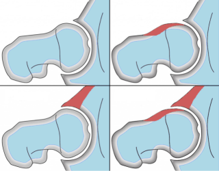
Figure 3: An illustration of femoroacetabular impingement (FAI). Top left: normal hip joint. Top right: cam type FAI. Bottom left: pincer type FAI. Bottom right: mixed type.

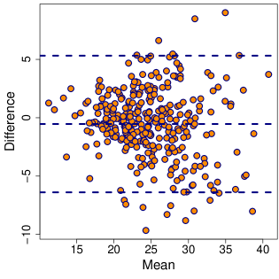
Figure 4: A Bland–Altman plot for the femoral cartilage data.

We applied our procedure for each of three choices of parametric marginal distribution: Gaussian, Laplace, and Student’s $t$ with noncentrality. The results are shown in Table 2, where the fourth and fifth columns give the estimated location and scale parameters for the three marginal distributions, the sixth column provides values of Akaike’s information criterion (AIC) (akaike1974new), and the final column shows model probabilities (burnham2011aic) relative to the $t$ model (since that model yielded the smallest value of AIC).

Marginal Model	$\hat{\omega}$	$\omega\in$	Location	Scale	AIC	Model Probability
Gaussian	0.837	(0.803, 0.870)	24.9	15.30	3,605	0.0002
Laplace	0.858	(0.829, 0.886)	24.0	14.34	3,643	$\approx$ 00001111
$t$	0.862	(0.833, 0.890)	23.3	11.21	3,588	11111
Empirical	0.846	(0.808, 0.869)	$-$	$-$	$-$	$-$1111

Table 2: Results from applying Sklar’s $\omega$ to the femoral-cartilage data.

We see that the estimates are comparable for the three choices of marginal distribution, yet the $t$ distribution is far superior to the others in terms of model probabilities. Figure 5 provides visual corroboration: it is clear that the $t$ assumption proves more appropriate because it is able to capture the mild asymmetry of the marginal distribution. The $t$ assumption also yielded the largest estimate of $\omega$ and the narrowest confidence interval (arrived at using the method of maximum likelihood). In any case, we must conclude that there is near-perfect agreement between raw T2* and contrast-enhanced T2*.

Note that, for a sufficiently large sample, it may be advantageous to employ a nonparametric estimate of the marginal distribution (see Section LABEL:inference for details). Results for this approach are shown in the final row of Table 2. We used a bootstrap sample size of 1,000 in computing the confidence interval. This yielded MCSEs smaller than 0.002.

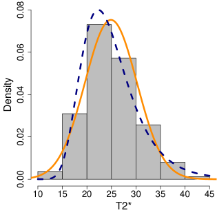
Figure 5: For the T2* data: histogram and fitted Gaussian and $t$ densities. The solid, orange curve is the fitted Gaussian density, and the dashed, blue curve is the fitted $t$ density.

A Krippendorff’s $\alpha$ analysis gave $\hat{\alpha}=0.837$ and $\alpha\in(0.802,0.864)$ ($n_{b}=$ 1,000; MSCEs $\approx$ 0.001). Since $\alpha$ implicitly assumes Gaussianity—$\alpha$ is the intraclass correlation for the ordinary one-way mixed-effects ANOVA model, and so $\hat{\alpha}$ is a ratio of sums of squares (artstein2008inter)—it is not surprising that the $\alpha$ results are quite similar to the results obtained by Sklar’s $\omega$ with Gaussian marginals.

3.3 Ordinal data from an imaging study of liver herniation

The data for this example, some of which are shown in Figure 6, are liver-herniation scores (in $\{1,\dots,5\}$) assigned by two coders (radiologists) to magnetic resonance images (MRI) of the liver in a study pertaining to congenital diaphragmatic hernia (CDH) (Danull). The five grades are described in Table 3.

	$u_{1}$	$u_{2}$	$u_{3}$	$u_{4}$	$u_{5}$	$\dots$	$u_{43}$	$u_{44}$	$u_{45}$	$u_{46}$	$u_{47}$
$c_{11}$	2	4	4	4	4	$\dots$	2	1	2	1	1
$c_{12}$	2	4	5	4	4	$\dots$	2	1	2	1	1
$c_{21}$	3	5	5	5	4	$\dots$	2	2	2	1	1
$c_{22}$	3	5	5	4	4	$\dots$	2	2	2	1	1

Figure 6: Ordinal scores for MR images of the liver. Each coder scored each unit twice.

Grade	Description
1	No herniation of liver into the fetal chest
2	Less than half of the ipsilateral thorax is occupied by the fetal liver
3	Greater than half of the thorax is occupied by the fetal liver
4	The liver dome reaches the thoracic apex
5	The liver dome not only reaches the thoracic apex but also extends across the thoracic midline

Table 3: Liver-herniation grades for the CDH study.

Each coder scored each of the 47 images twice, and so we are interested in assessing both intra-coder and inter-coder agreement. We can accomplish both goals with a single analysis by choosing an appropriate form for our copula correlation matrix $\mathbf{\Omega}$. Specifically, we let $\mathbf{\Omega}$ be block diagonal: $\mathbf{\Omega}=\mathop{\mathrm{diag}}(\mathbf{\Omega}_{i})$, where the block for unit $i$ is given by

$$𝛀{}_i=\begin{array}{ccccc}& c{}_{11}& c{}_{12}& c{}_{21}& c{}_{22}\\ c{}_{11}& 1& \omega {}_1& \omega {}_{12}& \omega {}_{12}\\ c{}_{12}& \omega {}_1& 1& \omega {}_{12}& \omega {}_{12}\\ c{}_{21}& \omega {}_{12}& \omega {}_{12}& 1& \omega {}_2\\ c{}_{22}& \omega {}_{12}& \omega {}_{12}& \omega {}_2& 1\end{array}$$