Generating Contradictory, Neutral, and Entailing Sentences

Abstract

Learning distributed sentence representations remains an interesting problem in the field of Natural Language Processing (NLP). We want to learn a model that approximates the conditional latent space over the representations of a logical antecedent of the given statement. In our paper, we propose an approach to generating sentences, conditioned on an input sentence and a logical inference label. We do this by modeling the different possibilities for the output sentence as a distribution over the latent representation, which we train using an adversarial objective. We evaluate the model using two state-of-the-art models for the Recognizing Textual Entailment (RTE) task, and measure the BLEU scores against the actual sentences as a probe for the diversity of sentences produced by our model. The experiment results show that, given our framework, we have clear ways to improve the quality and diversity of generated sentences.

1 Introduction

Algorithms designed to learn distributed sentence representations have been shown to be transferable across a range of tasks (Mou et al., 2016) and languages (Tiedemann, 2018). For example, Guu et al. (2017) proposed to represent sentences as vectors that encode a notion similarity between sentence pairs, and showed that vector manipulations of the representation can result in meaningful change in semantics. The question we would like to explore is whether the semantic relationship between sentence pairs can be modeled in a more explicit manner. More specifically, we want to model the logical relationship between sentences.

Controlling the logical relationship between sentences has many direct applications. First of all, we can use it to provide a more clear definition of paraphrasing. To do so, we require two simultaneous conditions: (i) that the input sentence entails the output sentence; and (ii) that the output sentence entails the input sentence.

$$\begin{split}&(\textsc{Sentence1}\models\textsc{Sentence2})\,\wedge\\ &\qquad(\textsc{Sentence2}\models\textsc{Sentence1})\end{split}$$ (1)

The first requirement ensures the output sentence cannot be false if the input sentence is true, so that the output sentence can be considered a fact expressed by the input sentence. The second requirement ensures that the output contains at least the input’s information. The two requirements together can be used to define semantic equivalence between sentence.

Another interesting application is multi-document summarization. Traditionally, to summarize multiple documents, one would expect the model to abstract the most important part of the source documents, and this is usually measured by the amount of overlap that the output document has with the inputs. Informally, one finds the maximal amount of information that has the highest precision with each source document. Alternatively, if one wants to automate news aggregation, the ideal summary would need to contain the same number of facts as are contained in the union of all source documents. We can think of this second objective as requiring that the output document entail every single sentence across all source documents.

In this paper, we propose an approach to generating sentences, conditioned on an input sentence and a logical inference label. We do this by modeling the different possibilities for the output sentence as a distribution over the latent representation, which we train using an adversarial objective.

In particular, we differ from the usual adversarial training on text by using a differentiable global representation. Architecture-wise, we also propose a Memory Operation Selection Module (MOSM) for encoding a sentence into a vector representation. Finally, we evaluate the quality and the diversity of our samples.

The rest of the paper is organized as follows: Sec. 2 will cover the related literature. Sec. 3 will detail the proposed model architecture, and Sec. 4 will describe and analyze the experiments run. Sec. 5 will then discuss the implications of being able to solve this task well, and the future research directions relating to this work. Finally, we conclude in Sec. 6.

2 Related Work

Many natural language tasks require reasoning capabiliities. The Recognising Textual Entailment (RTE) task requires the system to determine if the premise and hypothesis pair are (i) an entailment, (ii) contradicting each other or (iii) neutral to each other. The Natural language Inference (NLI) Task from Bowman et al. (2015a) introduces a large dataset with labeled pairs of sentences and their corresponding logical relationship. This dataset allows us to quantify how well current systems are able to be trained to recognise sentences with those relationships. Examples of the current state-of-the-art for this task include Chen et al. (2017) and Gong et al. (2017).

Here we are interested in generating natural language that satisfies the given textual entailment class. Kolesnyk et al. (2016) has attempted this using only sentences from the entailment class, and focusing on generating a hypothesis given the premise. Going in this direction results in removal of information from the premise sentence. In this paper, we focus on going in the other direciton: generating a premise from a hypothesis. This requires adding additional details to the premise which have to make sense in context. In order to produce sentences with extra details and without some other details, we suggest that a natural way to model this kind of structure is to impose a distribution over an intermediate distribution representing the semantic space of the premise sentence.

In the realm of learning representations for sentences, Kiros et al. (2015) has a popular method for learning representations called “skip-thought” vectors. These are trained by using the encoded sentence to predict the previous and next sentence in a passage. Conneau et al. (2017) specifically learned sentence representations from the SNLI dataset. They claim that using the supervised data from SNLI can outperform “skip-thought” representations on different tasks. There have also been several efforts towards learning a distribution over sentence embeddings. Bowman et al. (2015b) used Variational Autoencoders (VAEs) to learn Gaussian distributed word embeddings. Hu et al. (2017) use a combined VAE/GAN objective to produce a disentangled representation that can be used to modify some attributes like sentiment and tense.

There have also been forays into conditional distributions for sentences – which is what is required here. Both Gupta et al. (2017) and Guu et al. (2017) introduce models of the form $p(\mathbf{x}|\mathbf{z},\mathbf{x}^{\prime})$, where $\mathbf{x}$ is a paraphrase of $\mathbf{x}^{\prime}$, and $\mathbf{z}$ represents the variability in the output sentence. Guu et al. (2017) introduces $\mathbf{z}$ as an edit vector. However, because $\mathbf{z}$ has to be paired with $\mathbf{x}^{\prime}$ in order to generate the sentence, $\mathbf{z}$ serves a very different purpose, and cannot be considered a sentence embedding in its own right. Ideally, what we want is a distribution over sentence representations, each one mapping to a set of semantically similar sentences. This is important if we want the distribution to model the possibilities of concepts that correspond to the right textual entailment with the hypothesis.

3 Method

Some approaches map a sentence to a distribution in the embedding space (Bowman et al., 2015b). The assumption when doing this is that there is some uncertainty over the latent space when mapping from the sentence. Some approaches, like Hu et al. (2017) attempt to disentangle factors in the learnt latent variable space, so that modifying each dimension in the latent representation modifies sentiment or tense in the original sentence.

Figure 1: The conceptual graphical model behind the formulation of our model. The red arrow represents the inference path from $\phi$ to $\mathbf{z}$.

If we consider plausible premise sentences ${\boldsymbol{\phi}}$ given a hypothesis ${\boldsymbol{\eta}}$ and an inference label $\ell$, there are many possible solutions, of varying likelihoods. We can model this probabilistically as $p({\boldsymbol{\phi}}|{\boldsymbol{\eta}},\ell)$. In our model, we assume an underlying latent variable $\mathbf{z}$ that accounts for the variation in possible output sentences,

$$p({\boldsymbol{\phi}}|{\boldsymbol{\eta}},\ell)=\int p({\boldsymbol{\phi}}|\mathbf{z})p(\mathbf{z}|{\boldsymbol{\eta}},\ell)\mathrm{d}\mathbf{z}$$

Another assumption we make is that given ${\boldsymbol{\phi}}$, $\mathbf{z}$ is independent of ${\boldsymbol{\eta}}$ and $\ell$. The resulting graphical model associated with the above dependency assumptions are depicted in Figure 1.

In our proposed model, we take inspiration from the Adversarial Autoencoder (Makhzani et al., 2015), however our prior is conditioned on ${\boldsymbol{\eta}}$ and $\ell$. Zhang et al. (2017) also proposed a Conditional Adversarial Autoencoder for age progression prediction. In addition to the adversarial discriminator, our model includes a classifier on the representation and the hypothesis and label. A similar framework is also discussed in Salimans et al. (2016).

3.1 Architecture

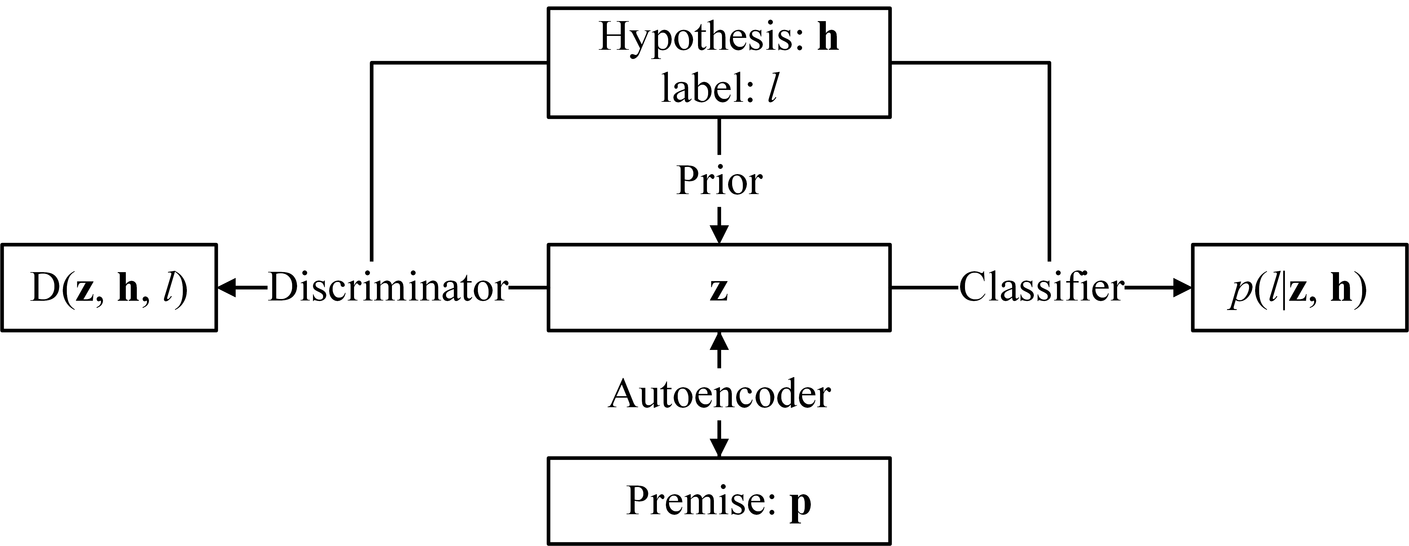
Figure 2: The architecture of the model. The autoencoder maps given premise ${\boldsymbol{\phi}}$ to a sentence representation $\mathbf{z}$, and reconstructs ${\boldsymbol{\phi}}$ from $\mathbf{z}$. Samples are drawn from the prior conditioned on ${\boldsymbol{\eta}}$ and $\ell$. The classifier takes $\mathbf{z}$ and ${\boldsymbol{\eta}}$ as input, and outputs probability of $l$. The discriminator takes $\mathbf{z}$, ${\boldsymbol{\eta}}$ and $l$ as input, and predicts whether $\mathbf{z}$ is given by the autoencoder or the prior.

The model consists of an encoder $q(\mathbf{z}|{\boldsymbol{\phi}})$, a conditional prior, $p(\mathbf{z}|{\boldsymbol{\eta}},\ell)$, a decoder $p({\boldsymbol{\phi}}|\mathbf{z})$, and a discriminator $\mathrm{D}(\mathbf{z},{\boldsymbol{\eta}},\ell)$.

Autoencoder

The autoencoder comprises of two parts. An encoder that maps the given premise ${\boldsymbol{\phi}}$ to a sentence representation $\mathbf{z}$, and a decoder that reconstructs ${\boldsymbol{\phi}}$ from a given $\mathbf{z}$. In our model, the encoder reads the input premise ${\boldsymbol{\phi}}=(x^{\boldsymbol{\phi}}_{1},...,x^{\boldsymbol{\phi}}_{|{\boldsymbol{\phi}}|})$ using an RNN network:

$$h^{\boldsymbol{\phi}}_{1},...,h^{\boldsymbol{\phi}}_{|{\boldsymbol{\phi}}|}=\mathrm{RNN}_{\mathrm{enc}}(x^{\boldsymbol{\phi}}_{1},...,x^{\boldsymbol{\phi}}_{|{\boldsymbol{\phi}}|})$$ (2)

and

$$\mathbf{z}=f_{\mathrm{compress}}(h^{\boldsymbol{\phi}}_{1},...,h^{\boldsymbol{\phi}}_{|{\boldsymbol{\phi}}|})$$ (3)

where $h_{t}\in\mathcal{R}^{n}$ is a hidden state at time $t$. $\mathbf{z}$ is a vector generated from sequence of the hidden states. We will call $f_{\mathrm{compress}}(\cdot)$ the compression function.

The decoder is trained to predict the next word $x^{\prime}_{t}$ given the sentence representation $\mathbf{z}$ and all the previously predicted words $(x^{\prime}_{1},...,x^{\prime}_{t-1})$. With an RNN, the conditional probability distribution of $x^{\prime}_{t}$ is modeled as:

$$p(x^{\prime}_{t}|x^{\prime}_{1},...,x^{\prime}_{t-1},\mathbf{z})=g(s_{t},c_{t})$$ (4)

and

$$s_{1},...,s_{|{\boldsymbol{\phi}}|}=\mathrm{RNN}_{\mathrm{dec}}(x^{\prime}_{1},...,x^{\prime}_{|{\boldsymbol{\phi}}|})$$ (5)

$$c_{t}=f_{\mathrm{retrieve}}(\mathbf{z},s_{t})$$ (6)

where $g(\cdot)$ is a nonlinear, potentially multi-layered, function that outputs the probability of $x^{\prime}_{t}$, $s_{t}$ is the hidden state of decoder RNN, and $f_{\mathrm{retrieval}}$ takes $s_{t}$ as the key to retrieve related information from $\mathbf{z}$. We note that other architectures such as a CNN or a transformer (Vaswani et al., 2017) can be used in place of the RNN. The details of the compression function and retrieval function will be discussed in Sec. 3.2.

Prior

We draw a sample, conditioned on $({\boldsymbol{\eta}},\ell)$, through the prior, which is described using following equations:

$$h^{\boldsymbol{\eta}}_{1},...,h^{\boldsymbol{\eta}}_{|{\boldsymbol{\eta}}|} = \mathrm{RNN}_{\mathrm{enc}}(x^{\boldsymbol{\eta}}_{1},...,x^{\boldsymbol{\eta}}_{|{\boldsymbol{\eta}}|})$$ (7)

$$\tilde{h}_{t} = \mathrm{MLP}([h^{\boldsymbol{\eta}}_{t},e_{\ell},\epsilon])$$ (8)

$$\hat{h}_{1},...,\hat{h}_{|{\boldsymbol{\eta}}|} = \mathrm{RNN}_{\mathrm{refine}}(\tilde{h}_{1},...,\tilde{h}_{|{\boldsymbol{\eta}}|})$$ (9)

$$\mathbf{z} = f_{\mathrm{compress}}(\hat{h}_{1},...,\hat{h}_{|{\boldsymbol{\eta}}|})$$ (10)

where $\epsilon$ is a random vector, $\epsilon_{i}\sim\mathcal{N}(0,1)$; $e_{\ell}$ is the label embedding and $[\cdot,\cdot]$ represents the concatenation of input vectors.

Classifier

This outputs the probability distribution over labels, taking as input the tuple $(\mathbf{z},{\boldsymbol{\eta}})$, and is described using the following equations:

$$h^{\boldsymbol{\eta}}_{1},...,h^{\boldsymbol{\eta}}_{|{\boldsymbol{\eta}}|} = \mathrm{RNN}_{\mathrm{enc}}(x^{\boldsymbol{\eta}}_{1},...,x^{\boldsymbol{\eta}}_{|{\boldsymbol{\eta}}|})$$ (11)

$$c_{t} = f_{\mathrm{retrieve}}(\mathbf{z},h^{\boldsymbol{\eta}}_{t})$$ (12)

$$\tilde{h}_{t} = \mathrm{MLP}([h^{\boldsymbol{\eta}}_{t},c_{t},||h^{\boldsymbol{\eta}}_{t}-c_{t}||,h^{\boldsymbol{\eta}}_{t}\odot c_{t}])$$ (13)

$$\hat{h}_{1},...,\hat{h}_{|{\boldsymbol{\eta}}|} = \mathrm{RNN}_{\mathrm{refine}}(\tilde{h}_{1},...,\tilde{h}_{|{\boldsymbol{\eta}}|})$$ (14)

$$\hat{h}_{\mathrm{max}} = \mathrm{Pooling}_{\mathrm{max}}(\hat{h}_{1},...,\hat{h}_{|{\boldsymbol{\eta}}|})$$ (15)

$$\hat{h}_{\mathrm{mean}} = \mathrm{Pooling}_{\mathrm{mean}}(\hat{h}_{1},...,\hat{h}_{|{\boldsymbol{\eta}}|})$$ (16)

$$p(\ell|\mathbf{z},{\boldsymbol{\eta}}) = \sigma(\mathrm{MLP}([\hat{h}_{\mathrm{max}},\hat{h}_{\mathrm{mean}}]))$$ (17)

where $\mathrm{Pooling}(\cdot)$ refers to an element-wise pooling operator, and the activation function $\sigma$ for output layer is the softmax function. The architecture of the classifier is inspired by (Chen et al., 2017). Instead of doing attention over the sequence of hidden states for the premise, we use the retrieval function in Equation 12 to retrieve related information $c_{t}$ in $\mathbf{z}$ for $h^{\boldsymbol{\eta}}_{t}$.

Discriminator

The discriminator takes as input $(\mathbf{z},{\boldsymbol{\eta}},\ell)$, and tries to determine if the $\mathbf{z}$ in question comes from the encoder or prior. The architecture of the discriminator is similar to that of the classifier, with the exception that Equation 13 is replaced by:

$$\tilde{h}_{t} = \mathrm{MLP}([h^{\boldsymbol{\eta}}_{t},c_{t},e_{\ell}])$$ (18)

to pass label information to the discriminator. The sigmoid function is used as the activation for the output layer.

In our model the autoencoder, prior and classifier share the same $\mathrm{RNN}_{\mathrm{enc}}(\cdot)$ parameters. The prior and the autoencoder share the same $f_{\mathrm{compress}}(\cdot)$ parameters. The classifier and the autoencoder share the same $f_{\mathrm{retrieve}}(\cdot)$ parameters. The discriminator does not share any parameters with the rest of model.

3.2 Compression and Retrieval Functions

The compression (Equation 3) and retrieval (Equation 6) functions can be modeled through many different mechanisms. Here, we introduce two different methods:

Mean Pooling

can be used to compress the sequence of the hidden states:

$$f_{\mathrm{compress}}(h_{1},...,h_{T})=\frac{1}{T}\sum_{t=1}^{T}h_{t}$$ (19)

and its retrieve counterpart directly returns $\mathbf{z}$:

$$f_{\mathrm{retrieve}}(\mathbf{z},s_{t})=\mathbf{z}$$ (20)

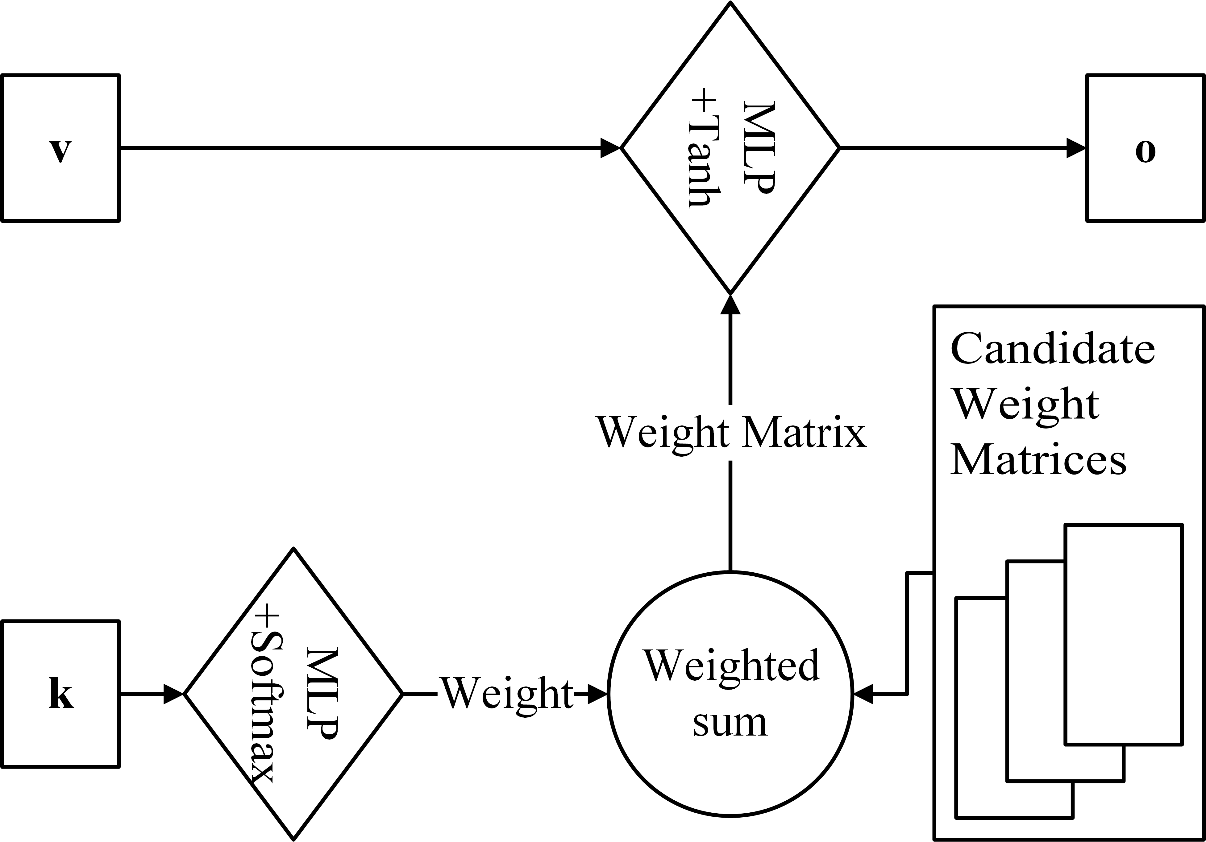
Figure 3: Memory Operation Selection Module takes a pair of vector $(\mathbf{k},\mathbf{v})$ as input, output a vector $\mathbf{o}$. $\mathbf{k}$ provide the control signal for the layer to compute a weighted sum of candidate weight matrices. The obtained matrix is used as the weight matrix in a normal feedforward layer, that takes $\mathbf{v}$ as input and outputs $\mathbf{o}$.

Memory Operation Selection Module (MOSM)

As an alternative to mean pooling, we use the architecture shown in Figure 3. A layer is defined as:

$$\gamma = \mathrm{softmax}(\mathbf{\Omega}\mathbf{k})$$ (21)

$$\tilde{\mathbf{W}} = \sum_{i=1}^{N_{\mathbf{W}}}\gamma_{i}\mathbf{W}_{i}$$ (22)

$$\mathbf{o} = \sigma(\tilde{\mathbf{W}}\mathbf{v})$$ (23)

where $\sigma$ can be any activation function, $\mathbf{v}$ is the input vector, $\mathbf{k}$ is the control vector, $\{\mathbf{W}_{i}\}$ are $N_{\mathbf{W}}$ candidate weight matrices. For convenience, we denote the MOSM function as $f_{\mathrm{MOSM}}(\mathbf{v},\mathbf{k})$.

Thus, we can define the MOSM compression method as:

$$f_{\mathrm{compress}}(h_{1},...,h_{T})=\tanh\left(\frac{1}{T}\sum_{t=1}^{T}f_{\mathrm{MOSM}}\left(h_{t},h_{t}\right)\right)$$ (24)

The compression function uses $\{h_{t}\}$ as both control and input vector, to write themselves into $\mathbf{z}$. Because different $h_{t}$s select different combinations of candidate matrices, we can have different mapping function each different $h_{t}$ at each time step.

$$f_{\mathrm{retrieve}}(\mathbf{z},s_{t})=f_{\mathrm{MOSM}}(\mathbf{z},s_{t})$$ (25)

Retrieval functions use $\{s_{t}\}$ as control vectors to retrieve information from $\mathbf{z}$. Since the layer generates a different weight matrix for the feedforward path for different $s_{t}$, we can output different $\mathbf{o}$ for the same $\mathbf{z}$.

3.3 Model Learning

Like most adversarial networks, the conditional adversarial autoencoder is trained with a gradient descent based method in two phases: the generative phase and the discriminative phase.

In the generative phase, the autoencoder is updated to minimize the reconstruction error of the premise. The classifier and the encoder are updated to minimize the classification error of the premise-hypothesis pair. The prior is also updated to optimize the classification error of $p(\ell|\mathbf{z},{\boldsymbol{\eta}})$, where $\mathbf{z}$ is draw from the prior. The encoder and the prior are updated to confuse the discriminator.

In our initial experiments, we found that the samples from just the adversarial training alone results in wildly varied output sentences. To ameliorate this, we propose an auxiliary loss:

$$\mathcal{L}_{\mathrm{auxiliary}}=\min_{i\in(1,...,N)}\{\mathrm{NLL}({\boldsymbol{\phi}}|\mathbf{z}_{i})\}\ ,\quad\mathbf{z}_{i}\sim p(\mathbf{z}|{\boldsymbol{\eta}},\ell)$$ (26)

where $N$ is the number of samples that are drawn from prior. The auxiliary loss measures how far our generated premises are from the true premise when conditioned on the hypothesis and label. As shown in experiment the model has better generating diversity, while more samples were drawn during training.

One can view this auxiliary loss as a ‘hard’ version of taking the log average of the probability of $N$ Monte-Carlo samples,

$$-\log\operatorname{\mathbb{E}}_{p(\mathbf{z}|{\boldsymbol{\eta}},\ell)}\left[p({\boldsymbol{\phi}}|\mathbf{z})\right]$$ (27)

$$~{}\approx-\log\frac{1}{N}\sum_{i}^{N}p({\boldsymbol{\phi}}|\mathbf{z}_{i}),\qquad\mathbf{z}_{i}\sim p(\mathbf{z}|{\boldsymbol{\eta}},\ell)$$ (28)

$$~{}=-\log\frac{1}{N}-\log\sum_{i}^{N}\exp\log p({\boldsymbol{\phi}}|\mathbf{z}_{i})$$ (29)

$$\leq-\log\frac{1}{N}+\min_{i\in(1,...,N)}-\log p({\boldsymbol{\phi}}|\mathbf{z}_{i})$$ (30)

Since $\log\frac{1}{N}$ is a constant, minimizing over the Equation 30 is the same as minimizing Equation 26.

In the discriminative phase, the discriminator is updated to tell apart the true $\mathbf{z}$ (generated using the prior) from the generated samples (given by autoencoder).

4 Experiments

We use the Stanford Natural Language Inference (SNLI) corpus (Bowman et al., 2015a) to train and evaluate our models. From our experiments, we want to determine two things. First, do the sentences produced by the model form the correct textual entailment class on which it was conditioned on? Second, is there diversity among the sentences that are generated?

4.1 Baseline Methods

For comparison, we use a normal RNN encoder-decoder as a baseline method. The model uses a bidirectional LSTM network as encoder. The encoder reads the input hypothesis into a sequence of hidden states $\{h_{t}\}$:

$$h^{\boldsymbol{\eta}}_{1},..,h^{\boldsymbol{\eta}}_{|{\boldsymbol{\eta}}|} = \mathrm{RNN}_{\mathrm{enc}}(x^{\boldsymbol{\eta}}_{1},..,x^{\boldsymbol{\eta}}_{|{\boldsymbol{\eta}}|})$$ (31)

$$z_{\boldsymbol{\eta}} = f_{\mathrm{compress}}(h^{\boldsymbol{\eta}}_{1},..,h^{\boldsymbol{\eta}}_{|{\boldsymbol{\eta}}|})$$ (32)

Where $f_{\mathrm{compress}}(\cdot)$ can be the mean method or an MOSM. The distributed representation of label $e_{\ell}$ and $z_{\boldsymbol{\eta}}$ are concatenated together to feed into a normal MLP network, which output the sentence representation $\mathbf{z}$:

$$\mathbf{z}=\mathrm{MLP}([z_{\boldsymbol{\eta}},e_{\ell}])$$ (33)

The decoder compute the conditional probability distribution with equations:

$$p(x^{\prime}_{t}|x^{\prime}_{1},...,x^{\prime}_{t-1})=g([s_{t},\mathbf{z}])$$ (34)

$$s_{t}=\mathrm{RNN}_{\mathrm{dec}}(x^{\prime}_{t-1},s_{t-1})$$ (35)

Thus, the baseline model share a similar architecture with prior and decoder in our model, while the randomness been toke out.

4.2 Experiment Settings

For all models, $\mathrm{RNN}_{\mathrm{enc}}$ and $\mathrm{RNN}_{\mathrm{refine}}$ are 2-layers bi-directional LSTM (Hochreiter & Schmidhuber, 1997), $\mathrm{RNN}_{\mathrm{dec}}$ are 2-layers uni-directional LSTM. The dimension of hidden state, embeddings and latent representation $\mathbf{z}$ are 300. When training, optimization is performed with Adam using learning rate $lr=0.001$, $\beta_{1}=0$, $\beta_{2}=0.999$ and $\sigma=10^{-8}$. We carry out gradient clipping with maximum norm $1.0$. We train each model for 30 epoch. For each iteration, we randomly choose to run the generative phase or discriminative phase with probability $0.5:0.5$. Since we didn’t observe significant benefit from using Beam Search, all premises are generated using greedy search.

4.3 Quality Evaluation

In order to evaluate the quality of the samples from our model, we trained two state-of-the-art models for SNLI: (1) Densely Interactive Inference Network (DIIN) (Gong et al., 2017), (2) Enhanced Sequential Inference Model (ESIM) (Chen et al., 2017).

In our experiments, we found that it is possible to achieve an accuracy of 68% on SNLI label prediction by training a classifier using only the hypothesis as input. This calls into question how much the classification models rely on just the hypothesis for performing its task. To investigate this phenomena further, we randomly permuted the premises of the original test set and passed these new (random) permis-hypothesis pairs to the classifiers. The results are shown in the row labelled Random in Table 1. We were satisfied that at 42.7% and 41.1%, the classification models (both DIIN and ESIM) were not relying entirely on the hypothesis for prediction.

Table 1: Classification accuracies for different state-of-the-art models on our samples. The row labeled Random we randomly permuted the premises of the original test set and ran them through the classifiers to test for the models’ reliance on just the hypothesis for classification.

Model	DIIN	ESIM
Random	42.7%	41.1%
Baseline (Mean)	59.6%	59.6%
Baseline (MOSM)	62.7%	62.6%
MOSM (N=1, -classifier)	67.2%	67.3%
MOSM (-auxiliary loss)	63.2%	60.6%
Mean (N=1)	64.4%	62.4%
Mean (N=10)	64.3%	62.3%
MOSM (N=1)	76.1%	75.9%
MOSM (N=10)	72.6%	71.8%

We sampled 9845 hypotheses from the test set, and produced ${\boldsymbol{\phi}}$ for each example with the given $\ell$. The $({\boldsymbol{\eta}},{\boldsymbol{\phi}},\ell)$ triplet was then passed to the classifiers and evaluated for accuracy. Both classification models perform at $\sim$88% accuracy, but, while they were not perfect, they provided a good probe for how well our models were generating the required sentences. Table 1 shows the accuracy of prediction on the respective models. Both the DIIN and ESIM models give similar results.

Our results show that using the MOSM gives an improvement over just taking the mean. Using the adversarial training also results in some gains, which suggests that training the model with the ‘awareness’ of the distribution over the representation space results in better quality samples. Using the adversarial training in conjunction with the MOSM layer gives us the model with the best performance. We also performed ablation tests, removing certain components of the model from the training to see how it affects the quality of samples. The difference between our best model against MOSM ($N=1$, -classifier) suggests that the classifier plays in important role in ensuring $\mathbf{z}$ is a representation in the right class. In our experiment removing the auxiliary loss, we still achieve an accuracy $\sim$61%. However, looking at the samples for this iteration of the model, while having some concepts in common with the hypothesis, the sentences in general are more nonsensical in comparison to those trained with the auxiliary loss (See an example in Figure 6).

Table 2: The confusion matrix for the samples from the best model MOSM ($N=1$)

Label \Pred.	Ent.	Neut.	Cont.
Entailment	67.8%	20.9%	11.4%
Neutral	6.6%	76.7%	16.7%
Contradiction	2.9%	12.8%	84.4%

The confusion matrix produced when evaluating our best model (MOSM, $N=1$) on DIIN shows us where the classification model and our generative model agree (See Table 2). In our Random experiments, we find that the model has a bias towards predicting contradictions. This is observed here as well, with contradictions being the category with the highest agreement. We therefore cannot conclude that contradictions are easier for our model to generate. Also, using the original test set, the category in which DIIN performs the best is entailment, with a precision of 89.1% compared to 84.3% for neutral and 88.4% for contradiction. This suggests that generating suitable premises that entail the hypothesis is the hardest task for the model.

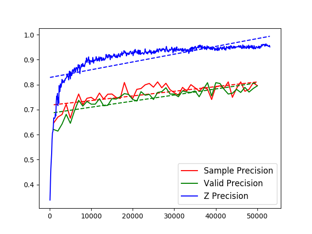
Figure 4: Different classification precisions given by our classifier in our model (MOSM, N=10) during training. Sample Precision shows the probability that classifier predicts correct label for generated premise and related real hypothesis. Valid precision shows the probability that classifier predicts correct label for real premise and real hypothesis. Z precision shows the probability that the feedforward network $f_{\mathrm{classifier}}(\mathbf{z},z_{\boldsymbol{\eta}})$ predicts correct label $\ell$, for given ${\boldsymbol{\eta}}$, $\ell$ and $\mathbf{z}$ drawn from prior $p(\mathbf{z}|{\boldsymbol{\eta}},\ell)$.

We also want to study how the classifier component of our model affects the generation of good samples. As shown in Figure 4, “Z precision” is higher then $0.9$. This suggests that the classifier provides a strong regularization signal to the sentence representation $\mathbf{z}$. Because the autoencoder is not perfect, we do not observe the the same sample classification precision after $\mathbf{z}$ is decoded. However, we still observe a synchronous improvement of both sample and valid precision. It is therefore reasonable to expect that a better classifier and a better autoencoder would result in better generated premises.

4.4 Diversity Evaluation

In order to evaluate the diversity of samples given by our model, we compute the BLEU score between to premises generated conditioned on the same hypothesis and label. In other words, given a triple $({\boldsymbol{\phi}}_{i},{\boldsymbol{\eta}}_{i},\ell_{i})$ from test set, we draw two different samples $(\mathbf{z}_{i1},\mathbf{z}_{i2})$ from the prior distribution $p(\mathbf{z}|{\boldsymbol{\eta}}_{i},\ell_{i})$. Then the decoder generates two premises $({\boldsymbol{\phi}}_{i1},{\boldsymbol{\phi}}_{i2})$ using greedy search conditioned on $(\mathbf{z}_{i1},\mathbf{z}_{i2})$ respectively. The similarity score between generated premises is then estimated by:

$$\mathrm{BLEU}_{i}=\frac{1}{2}\left(\mathrm{BLEU}(\mathbf{z}_{i1},\mathbf{z}_{i2})+\mathrm{BLEU}(\mathbf{z}_{i2},\mathbf{z}_{i1})\right).$$ (36)

For comparison, we also compute the BLEU score between real premise and generated premise $({\boldsymbol{\phi}}_{i},{\boldsymbol{\phi}}_{i1})$. The average of diversity score between two generated premises is noted as $\mathrm{BLEU}_{\mathrm{SS}}$, the one between real and generated premises is noted as $\mathrm{BLEU}_{\mathrm{RS}}$. Since it is not necessary have n-gram match between premises, BLEU score can be inaccurate on some data points. We employ the Smoothing technique 2 described in Chen & Cherry (2014).

Table 3: BLEU score for different models

Model	$\mathrm{BLEU}_{\mathrm{RS}}$	$\mathrm{BLEU}_{\mathrm{SS}}$
Baseline (Mean)	14.4	N/A
Baseline (MOSM)	14.7	N/A
MOSM (N=1, -classifier)	14.4	46.7
MOSM (-auxiliary loss)	10.3	14.8
Mean (N=1)	11.9	27.9
Mean (N=10)	11.3	17.3
MOSM (N=1)	14.2	38.9
MOSM (N=10)	13.2	22.5

As shown in Table 3, when we increase the number of samples $N$ in the auxiliary loss, the diversity of samples increases for both mean pooling and MOSM. This can serve as empirical evidence that the diversity of our model can be controlled by choosing a different hyper-parameter $N$. The higher $\mathrm{BLEU}_{\mathrm{RS}}$ given by MOSM method could be interpreted as real premise is more close to the center of mass of prior distribution. We also observe a gap between $\mathrm{BLEU}_{\mathrm{RS}}$ and $\mathrm{BLEU}_{\mathrm{SS}}$. The gap shows that the sampled premise is still relatively similar between themselves. After removing the classifier, we observe an increase in $\mathrm{BLEU}_{\mathrm{SS}}$. One possible explanation is that classifier prevents the prior from overfitting the training data. We observe an decrease in both BLEU scores, after removing the auxiliary loss. However, Table 1 and Figure 6 shows that removing auxiliary loss give low quality samples.

Figure 5: Visualization of the effect of auxiliary loss with multiple samples. For a pair of $({\boldsymbol{\phi}},{\boldsymbol{\eta}})$, we repeat 100 times the process of compute auxiliary loss (N=10) in Equation 26. Blue points represent $\mathbf{z}_{i}$ selected by minimum function, green points represent $\mathbf{z}_{i}$ that are not selected. Our model (MOSM, N=10) is used for computing $\mathbf{z}$ and perplexities. t-SNE is used to visualize high-dimensional data (Maaten & Hinton, 2008).

While the auxiliary loss is essential for the prior and the decoder to learn to cooperate, using an auxiliary loss where $(N=1)$ will collapse the prior distribution; instead of a distribution, the prior will learn to ignore the random input and deterministically predict $\mathbf{z}$. As shown in Figure 5, the auxiliary loss $(N=10)$ only passes gradients to the $\mathbf{z}$s in the left region of the distribution. As a result, samples drawn from right region have a significant lower chance receive gradient from decoder, while the entire region receives gradients from the discriminator and classifier. Therefore, the prior distribution can expand to more regions, but only those regulated by discriminator and classifier. This will increase the diversity of samples. However, we also observe that the precision slightly decreases in Table 1. This suggests that the discriminator and classifier in our model are not perfect for regularizing the prior distribution.

4.5 Samples

Samples from MOSM (N=10)

H: a worker stands over a bread display .

L: Entailment

S1: a man in a blue shirt is preparing food in a kitchen .

S2: a man in a blue shirt is washing a window .

H: there is a jockey riding a horse .

L: Entailment

S1: a horse rider on a bucking horse .

S2: a jockey riding a horse in a rodeo .

H: a man sitting on the couch reading a book .

L: Contradiction

S1: a man is sitting on a bench with his hands in his pockets .

S2: a man in a blue shirt is standing in front of a store .

H: a baby in his stroller outside .

L: Contradiction

S1: a woman is sitting on a bench next to a baby .

S2: a woman is sitting on a bench in a park .

H: the man is being watched .

L: Neutral

S1: a man jumps from a bridge for an elderly couple at a beach .

S2: a man in a blue shirt is standing in front of a building .

H: there is a human selling hot dogs .

L: Neutral

S1: a person is standing in front of a food cart .

S2: a woman in a white shirt is standing in front of a counter selling food .

 

Samples from MOSM (-auxiliary loss)

H: a restaurant prepares for a busy day .

L: Neutral

S1: a pink teenager prepares on a tune on the roots .

S2: a UNK restaurant dryer for a canvas .

Figure 6: Example sentence generated by our model (MOSM, N=10). H is the hypothesis, L is the label, S1 is the first sample, and S2 is the second sample. The samples shown below the line are drawn from a model trained without the auxiliary loss.

Figure 6 shows several examples generated by our model (MOSM, N=10). These example shows that our model can generate a variety of different premise while keep the correct semantic relation. Some of subjects in hypothesis are correctly replace by synonyms (e.g. “jocky” is replaced by “horse rider”, “human” is replaced by “person” and “woman”). The model also get some potential logical relation correct (e.g. “reading a book” is contradicted by “with his hands in his pockets”, “stands over a bread display” can either means “washing a window” or “preparing food in a kitchen”).

However, we also observe that the model tries to add “a blue shirt” for most “man”s in the sentences, which is one of the easiest way to add extra information into the model. The phenomenon aligned with well-known model collapse failure case for most adversarial training based method. This observation give an explanation for the relatively higher BLEU between sample. The model also have some bias while generating premise (e.g. when hypothesis mention “a baby”, the premise automatically mention “a woman”), which aligns with the recent discovery that visual recognition tasks model tend to output biased predictions (Zhao et al., 2017).

5 Discussion

The broader vision of our project is to attain logical control for language, which we believe will allow us to perform better across many natural language applications. This is most easily achieved at the word-level, by adding or removing specific words to a sentence, using word generation rules based on language-specific grammars. However, just as distributed word representations can be meaningfully combined (Mikolov et al., 2013) with good outcomes, we believe that sentence-level representations are the way forward for manipulation of text.

The kind of control we seek to model, specifically, is characterized by the logical relationships between sentence pairs. Controlling semantic representation by modeling logical relationship between the input and output sentences has many potential use cases. Returning to the task of multi-document summarization discussed in the introduction, operating in the semantic space allows one to abstract the information of a document. Controlling the logical relationships among sentences provides a new way to think about what a summary is. Ideally, when multiple sources of information are given, we would like the output summary ${\boldsymbol{\phi}}$ generated by a machine to be entailable by the union of inputs $(\cup_{j\in\mathcal{J}}{\boldsymbol{\eta}}_{j})\models{\boldsymbol{\phi}}$ . This addresses the problem of precision: the resulting summary now has a subset of the information available in the union of all the given hypotheses.

To address the problem of recall, we need the resulting summary to entail each one of the individual hypotheses: $\wedge_{i}({\boldsymbol{\phi}}\models{\boldsymbol{\eta}}_{j})$ Together, these two criteria form a clear formal definition for multi-document summarization,

$$\{\,{\boldsymbol{\phi}}\,:\,\wedge_{i}({\boldsymbol{\phi}}\models{\boldsymbol{\eta}}_{j})\,\wedge\,\,(\cup_{j\in\mathcal{J}}{\boldsymbol{\eta}}_{j})\models{\boldsymbol{\phi}}\,\}$$

which represents the set of all possible ${\boldsymbol{\phi}}$ that fit the criteria.

In our paper, we toyed with the possibility of modeling the set $\{\,{\boldsymbol{\phi}}\,:\,{\boldsymbol{\phi}}\models{\boldsymbol{\eta}}\,\}$ by training a model with a distribution over different premises in the latent space $\mathbf{z}$. A good subsequent step would be modelling the first part of our logical description of multi-document summarisation,

$$\{\,{\boldsymbol{\phi}}\,:\,\wedge_{i\in\mathcal{J}}({\boldsymbol{\phi}}\models{\boldsymbol{\eta}}_{j})\,\}=\cap_{i\in\mathcal{J}}\{\,{\boldsymbol{\phi}}\,:\,{\boldsymbol{\phi}}\models{\boldsymbol{\eta}}_{j}\,\}$$

This suggests a possible avenue for producing such a premise is finding the intersection of the distribution over $\mathbf{z}$ for two given hypotheses that are likely enough to occur.

Future work can explore the possibility of this and determining the union of the hypotheses entailing the given premise.

6 Conclusion

We have proposed a model that generates premises from hypotheses with an intermediate latent space, which we interpret as different possible premises for a given hypothesis. This was trained using a Conditional Adversarial Autoencoder. This paper also proposed the Memory Operation Selection Module for encoding sentences to a distributed representation that uses attention over different operations in order to encode the input. The model was evaluated for quality and diversity. In terms of quality, we used two state-of-the-art models for the RTE task on SNLI, and the samples generated by our best model were able to achieve an accuracy of 76.1%. For diversity, we compared the BLEU scores between the real premises and the generated premises, and the BLEU scores between the generated premises. In this regard, while our model is able to generate different premises for each hypothesis, there is still a gap between when compared to the similarities to the real premises. Looking at the samples, we note that the additional details that our model generates tend to repeat, and correspond to some type of mode collapse.

The task of performing reasoning well with natural language still remains a challenging problem. Our experiments demonstrate that while we can generate sentences with the logical entailment properties we desire, there is still much to be done in this direction. We hope with the new lens on some NLP tasks as natural language manipulation with logical control, new perspectives and methods will emerge to improve the field.

References

- Bowman et al. (2015a) Bowman, Samuel R., Angeli, Gabor, Potts, Christopher, and Manning, Christopher D. A large annotated corpus for learning natural language inference. In Proceedings of the 2015 Conference on Empirical Methods in Natural Language Processing (EMNLP). Association for Computational Linguistics, 2015a.
- Bowman et al. (2015b) Bowman, Samuel R, Vilnis, Luke, Vinyals, Oriol, Dai, Andrew M, Jozefowicz, Rafal, and Bengio, Samy. Generating sentences from a continuous space. arXiv preprint arXiv:1511.06349, 2015b.
- Chen & Cherry (2014) Chen, Boxing and Cherry, Colin. A systematic comparison of smoothing techniques for sentence-level bleu. In Proceedings of the Ninth Workshop on Statistical Machine Translation, 2014.
- Chen et al. (2017) Chen, Qian, Zhu, Xiaodan, Ling, Zhen-Hua, Wei, Si, Jiang, Hui, and Inkpen, Diana. Enhanced lstm for natural language inference. In Proceedings of the 55th Annual Meeting of the Association for Computational Linguistics (Volume 1: Long Papers), volume 1, 2017.
- Conneau et al. (2017) Conneau, Alexis, Kiela, Douwe, Schwenk, Holger, Barrault, Loic, and Bordes, Antoine. Supervised learning of universal sentence representations from natural language inference data. arXiv preprint arXiv:1705.02364, 2017.
- Gong et al. (2017) Gong, Yichen, Luo, Heng, and Zhang, Jian. Natural language inference over interaction space. arXiv preprint arXiv:1709.04348, 2017.
- Gupta et al. (2017) Gupta, Ankush, Agarwal, Arvind, Singh, Prawaan, and Rai, Piyush. A deep generative framework for paraphrase generation. arXiv preprint arXiv:1709.05074, 2017.
- Guu et al. (2017) Guu, Kelvin, Hashimoto, Tatsunori B, Oren, Yonatan, and Liang, Percy. Generating sentences by editing prototypes. arXiv preprint arXiv:1709.08878, 2017.
- Hochreiter & Schmidhuber (1997) Hochreiter, Sepp and Schmidhuber, Jürgen. Long short-term memory. Neural computation, 1997.
- Hu et al. (2017) Hu, Zhiting, Yang, Zichao, Liang, Xiaodan, Salakhutdinov, Ruslan, and Xing, Eric P. Toward controlled generation of text. In International Conference on Machine Learning, 2017.
- Kiros et al. (2015) Kiros, Ryan, Zhu, Yukun, Salakhutdinov, Ruslan R, Zemel, Richard, Urtasun, Raquel, Torralba, Antonio, and Fidler, Sanja. Skip-thought vectors. In Advances in neural information processing systems, 2015.
- Kolesnyk et al. (2016) Kolesnyk, Vladyslav, Rocktäschel, Tim, and Riedel, Sebastian. Generating natural language inference chains. arXiv preprint arXiv:1606.01404, 2016.
- Maaten & Hinton (2008) Maaten, Laurens van der and Hinton, Geoffrey. Visualizing data using t-sne. Journal of machine learning research, 2008.
- Makhzani et al. (2015) Makhzani, Alireza, Shlens, Jonathon, Jaitly, Navdeep, Goodfellow, Ian, and Frey, Brendan. Adversarial autoencoders. arXiv preprint arXiv:1511.05644, 2015.
- Mikolov et al. (2013) Mikolov, Tomas, Sutskever, Ilya, Chen, Kai, Corrado, Greg S, and Dean, Jeff. Distributed representations of words and phrases and their compositionality. In Advances in neural information processing systems, 2013.
- Mou et al. (2016) Mou, Lili, Meng, Zhao, Yan, Rui, Li, Ge, Xu, Yan, Zhang, Lu, and Jin, Zhi. How transferable are neural networks in nlp applications? arXiv preprint arXiv:1603.06111, 2016.
- Salimans et al. (2016) Salimans, Tim, Goodfellow, Ian, Zaremba, Wojciech, Cheung, Vicki, Radford, Alec, and Chen, Xi. Improved techniques for training gans. In Advances in Neural Information Processing Systems, 2016.
- Tiedemann (2018) Tiedemann, Jörg. Emerging language spaces learned from massively multilingual corpora. arXiv preprint arXiv:1802.00273, 2018.
- Vaswani et al. (2017) Vaswani, Ashish, Shazeer, Noam, Parmar, Niki, Uszkoreit, Jakob, Jones, Llion, Gomez, Aidan N, Kaiser, Łukasz, and Polosukhin, Illia. Attention is all you need. In Advances in Neural Information Processing Systems, 2017.
- Zhang et al. (2017) Zhang, Zhifei, Song, Yang, and Qi, Hairong. Age progression/regression by conditional adversarial autoencoder. In The IEEE Conference on Computer Vision and Pattern Recognition (CVPR), volume 2, 2017.
- Zhao et al. (2017) Zhao, Jieyu, Wang, Tianlu, Yatskar, Mark, Ordonez, Vicente, and Chang, Kai-Wei. Men also like shopping: Reducing gender bias amplification using corpus-level constraints. arXiv preprint arXiv:1707.09457, 2017.