A Neural Network Approach to Missing Marker Reconstruction in Human Motion Capture

Abstract.

Optical motion capture systems have become a widely used technology in various fields, such as augmented reality, robotics, movie production, etc. Such systems use a large number of cameras to triangulate the position of optical markers. The marker positions are estimated with high accuracy. However, especially when tracking articulated bodies, a fraction of the markers in each timestep is missing from the reconstruction.

In this paper, we propose to use a neural network approach to learn how human motion is temporally and spatially correlated, and reconstruct missing markers positions through this model. We experiment with two different models, one LSTM-based and one time-window-based. Both methods produce state-of-the-art results, while working online, as opposed to most of the alternative methods, which require the complete sequence to be known. The implementation is publicly available at https://github.com/Svito-zar/NN-for-Missing-Marker-Reconstruction.

1. Introduction

Often a digital representation of human motion is needed. This representation is useful in a wide range of scenarios: mapping an actor performance to a virtual avatar (in movie productions or in the game industry); predicting or classifying a motion (in robotics) ; trying clothes in a digital mirror; etc.

A common way to obtain this digital representation is marker-based optical motion capture (mocap) systems. Such systems use a large number of cameras to triangulate the position of optical markers.These are then used to reconstruct the motion of the objects to which the markers are attached.

All motion capture systems suffer to a higher or lower degree from missing marker detections, due to occlusion problems (less than two cameras see the marker) or marker detection failures.

In this paper, we propose a method for reconstruction of missing markers to create a more complete pose estimate (see Figure 1). The method exploits knowledge about spatial and temporal correlation in human motion, learned from data examples to remove position noise and fill in missing parts of the pose estimate (Section 3).

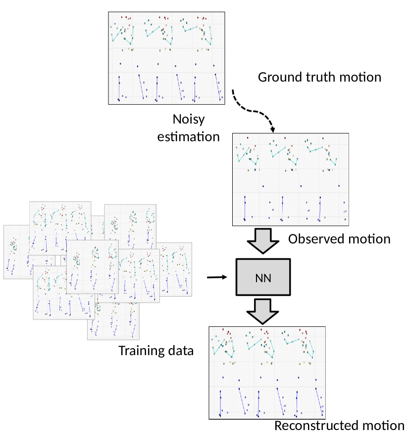
Figure 1. Illustration of our method for missing marker reconstruction. Due to errors in the capturing process, some markers are not captured. The proposed method exploits spatial and temporal correlations to reconstruct the pose of the missing markers.

A number of methods have been proposed within the Graphics community to address the problem of missing marker reconstruction. The traditional approach (Burke and Lasenby, 2016; Peng et al., 2015) is interpolation within the current sequence. Wang et al proposed a method which exploits motion examples to learn typical correlations (Wang et al., 2016b). The novelty of our method with respect to theirs is that while they learn linear dependencies, we employ a Neural Network (NN) methodology which enables modeling of more complicated spatial and temporal correlations in sequences of a human pose.

In Section  6 we demonstrate the effectiveness of our network, showing that our method outperforms the state of the art in missing marker reconstruction in various conditions.

Finally, we discuss our results in Section 7.

2. Related work

The task of modeling human motion from mocap data has been studied quite extensively in the past. We here give a short review of the works most related to ours.

2.1. Missing Marker Reconstruction

It is possible to do 3D pose estimation even with affordable sensors such as Kinect. However, all motion capture systems suffer to some degree from missing data. This has created a need for methods for missing marker reconstruction.

The missing marker problem has been traditionally formulated as a matrix completion task. Peng et al. (Peng et al., 2015) solve it by non-negative matrix factorization, using the hierarchy of the body to break the motion into blocks. Wang et al. (Wang et al., 2016b) follow the idea of decomposing the motion and do dictionary learning for each body part. They train their system separately for each type of motion. Burke and Lasenby (Burke and Lasenby, 2016) apply PCA first and do Kalman smoothing afterward, in the lower dimensional space. Gloersen and Federolf (Gløersen and Federolf, 2016) used weighted PCA to reconstruct markers. Taylor et al. (Taylor et al., 2007) applied Condition Restricted Boltzmann Machine based on the binary variables. Both Taylor (Taylor et al., 2007) and Gloersen(Gløersen and Federolf, 2016) were limited to cyclic motions, such as walking and running. All those methods are based on linear algebra. They make strong assumptions about the data: each marker is often assumed to be present at least at one time-step in the sequence. Moreover, due to the linear models, they often struggle to reconstruct irregular and complex motion.

The limitations discussed above motivate the neural network approach to the missing marker problem. Mall et al. (Mall et al., 2017) successfully applied deep neural network based on the bidirectional LSTM to denoise human motion and recover missing markers. Our approach is similar to theirs, but we are using a simpler network, which requires less data and computational resources. We also experiment with two different ways to handle the sequential character of the problem, while they just choose one approach.

2.2. Denoising

Another related task which can be tackled with our networks is removing additive noise from the marker data. Recently Holden (Holden, 2018) used a similar approach to this problem. He employed a neural network that took noisy markers as an input and returned clean body position as an output. The main difference is that our network is also capable of reconstructing missing values and takes sequential information into account.

2.3. Prediction

A highly related problem is to predict human motion some time into the future.

State-of-the-art methods try to ensure continuity either by using Recurrent Neural Networks (RNNs) (Fragkiadaki et al., 2015; Jain et al., 2016) or by feeding many time-frames at the same time (Bütepage et al., 2017). While our focus is not on prediction, our networks architectures are inspired by those methods.

Since our application is not a prediction, our architecture is slightly different.

Another related paper is the work of Bütepage et al. (Bütepage et al., 2017), who use a sliding window and a Fully Connected Neural Network (FCNN) to do motion prediction and classification. Again, since our problem is different, we modify their network, using a much shorter window length, fewer layers, and no bottleneck.

3. Method overview

In the following section, we give a mathematical problem formulation and an overview of the proposed approach.

3.1. Missing Markers

Missing markers in real life correspond to the failure of a sensor in the motion capture system.

In our experiments, we use mocap data without missing markers. Missing markers are emulated by nullifying some marker positions in each frame. This process can be mathematically formulated as a multiplication of the mocap frame $\mathbf{x}_{t}$ by a binary matrix $M_{t}$:

(1) $$\mathbf{\hat{x}}_{t}=C(\mathbf{x}_{t})=M_{t}\mathbf{x}_{t},$$

where $M_{t}\in[0,1]^{3nx3n}$, such that that all 3 coordinates of any marker are either missing or present at the same time.

Every marker is missing over a few time-frames. The percentage of missing values is usually referred to as the missing rate.

3.2. Missing Marker Reconstruction as Function Approximation

Missing marker reconstruction is defined in the following way: Given a human motion sequence $\mathbf{\hat{x}}$ corrupted by missing markers, the goal is to reconstruct the true pose $\mathbf{x}_{t}$ for every frame $t$.

We approach missing markers reconstruction as a function approximation problem: The goal is to learn a reconstruction function $R$ that approximates the inverse of the corruption function $C$ in Eq. (3). This function would map the sequence of corrupted poses to an approximation of the true poses:

(2) $$\mathbf{x}=R(\mathbf{\hat{x}})\approx C^{-1}(\mathbf{\hat{x}})$$

The mapping $C$ is under-determined, so it is not invertible. However, it can be approximated by learning spatial and temporal correlations in human motion in general, from a set of other pose sequences.

We propose to use a Neural Network (NN) approach to learn $R$, well known for being a powerful tool for function approximation (Hornik et al., 1989). We employ two different types of neural network models, which are described in the following sections. Both of them are using a principle of Denoising Autoencoder (Vincent et al., 2008): during the training Gaussian additive noise was injected into the input:

(3) $$\mathbf{\hat{x}}_{t}=\hat{C}(\mathbf{x}_{t})=M_{t}(\mathbf{x}_{t}+\mathcal{N}(0,\sigma(X)*\alpha)),$$

where $\sigma(X)$ is a standard deviation in the training dataset and $\alpha$ is a coefficient of proportionality, which we call the noise parameter. It was experimentally set to the value of 0.3.

Denoising is commonly used to regularize encoder-decoder NN. Experiments proved it to be beneficial in our application as well.

The network was learning to remove noise, at the same time as reconstructing missing values. During the testing, no noise was injected. Our two methods are compared to each other and to the state of the art in missing marker reconstruction in Section 6.

4. Neural Network Architectures

In this section, the two versions of the method are explained.

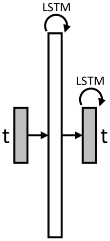
(a) LSTM-based

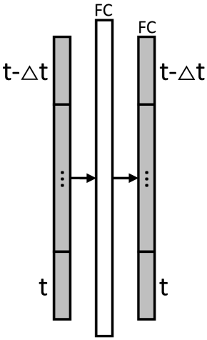
(b) Window-based

Figure 2. Illustration of the two architecture types. (a) LSTM-based architecture (Section 4.1). (b) Window-based architecture (Section 4.2).

4.1. LSTM-Based Neural Network Architecture

Long-Short Term Memory (LSTM) (Hochreiter and Schmidhuber, 1997) is a special type of Recurrent Neural Network (RNN). It was designed as a solution to the vanishing gradient problem (Hochreiter, 1998) and has become a default choice for many problems that involve sequence-to-sequence mapping (Sutskever et al., 2014; Donahue et al., 2015; Shi et al., 2017).

Our network is based on LSTM and illustrated in Figure 2a. The input layer is a corrupted pose $\mathbf{\hat{x}}_{t}$, and the output LSTM layer is the corresponding true pose $\mathbf{x}_{t}$.

4.2. Window-based Neural Network architecture

An alternative approach is to use a range of previous time-steps explicitly, and to train a regular Fully Connected Neural Network (FCNN) with the current pose along with a short history, i.e., a window of poses over time $(t-\Delta t):t$.

This network is illustrated in Figure 2b. The input layer is a window of concatenated corrupted poses $[\mathbf{\hat{x}}^{T}_{t-\Delta t},...,\mathbf{\hat{x}}^{T}_{t}]^{T}$. The output layer is the corresponding window of true poses $[\mathbf{x}^{T}_{t-\Delta t},...,\mathbf{x}^{T}_{t}]^{T}$. In between, there are a few hidden fully connected layers.

This structure is inspired by the sliding time window-based method of Bütepage et al. (Bütepage et al., 2017), but is adapted to pose reconstruction. For example, there is no bottleneck middle layer and fewer layers in general, to create a tighter coupling between the corrupted and real pose, rather than learning a high-level and holistic mapping of a pose. We also use window length T=10, instead of 100, based on the performance on the validation dataset.

5. Dataset

We evaluate our method on the popular benchmark CMU Mocap dataset (CMU, 2003). This database contains 2235 mocap sequences of 144 different subjects. We use the recordings of 25 subjects, sampled at the rate of 120 Hz, covering a wide range of activities, such as boxing, dancing, acrobatics and running.

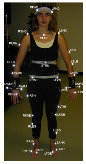
Figure 3. Marker placement in the CMU Mocap dataset (mocap.cs.cmu.edu).

5.1. Preprocessing

We start preprocessing by transforming every mocap sequence into the hips-center coordinate system. First joint angles from the BVH file are transformed into the 3D coordinates of the joints. The 3D coordinates are translated to the center of the hips by subtracting hip coordinates from each marker. We then normalize the data into the range [-1,1] by subtracting the mean pose over the whole dataset and then dividing all values by the absolute maximal value in the dataset.

5.2. Data Explanation

The CMU dataset contains 3D positions of a set of markers, which were recorded by the mocap system at CMU. Example of a marker placement during the capture can be seen in Figure 3. All details can be found in the dataset description (CMU, 2003).

The human pose at each time-frame $t$ is represented as a vector of the marker 3D coordinates: $\mathbf{x}_{t}=[x_{i,t},y_{i,t},z_{i,t}]_{i=1:n}$, where $n$ denotes the number of markers used during the mocap collection. In the CMU data, $n=41$, and the dimensionality of a pose is $3n=123$.

A sequence of poses is denoted $\mathbf{x}=[\mathbf{x}_{t}]_{t=1:T}$.

5.3. Training, Validation, and Test Data Configurations

The validation dataset contains 2 sequences from each of the following motions: pantomime, sports, jumping, and general motions . The test dataset contains basketball, boxing and jump turn sequences. The training dataset contains all the sequences not used for validation or testing, from 25 different folders in the CMU Mocap Dataset, such as 6, 14, 32, 40, 141, 143, which include testing types as well.

Subjects from the training dataset were also present in the test and validation datasets. Generalization to the novel subjects and motion types was tested experimentally.

6. Experiments

We use the commonly used (Peng et al., 2015; Wang et al., 2016b; Burke and Lasenby, 2016) Root Mean Squared Error (RMSE) over the missing markers to measure reconstruction error.

Implementation Details: All methods were implemented using Tensorflow(Abadi et al., 2016). The code is publicly available.

For training purposes, we extract short sequences from the dataset by sliding window, then shuffle them and feed to the network. The training was done using the Adam optimizer (Kingma and Ba, 2014) with a batch size of 32.

The hyperparameters for both architectures were optimized w.r.t. the validation dataset (Section 5.3) using grid search. Table 1 contains the main hyper-parameters.

Table 1. Hyperparameters for our NNs.
$\alpha$ is initial learning rate, $\Delta t$ is sequence length.

NN-type	Width	Depth	Dropout	$\alpha$	$\Delta t$
LSTM	1024	2	0.9	0.0002	64
Window	512	2	0.9	0.0001	20

6.1. Comparison to the State of the Art

First of all, the models presented above are evaluated in the same setting as most of the other random missing marker reconstruction methods. A specific amount of random markers (10%, 20%, or 30%) are removed over a few time-frames and each method is applied to recover them. The length of the gap was sampled from the Gaussian distribution with mean 10 and standard deviation 5, following the state-of-the-art settings (Wang et al., 2016b). The reconstruction error is measured.

There is randomness in the system; in the initialization of the network weights and choosing missing markers. Therefore, every experiment is repeated 3 times and error mean and standard deviation are measured.

Tables 2c provide the comparison of the performance of our system with 3 state-of-the-art papers and with the simplest solution (linear interpolation) as a baseline, on 3 action classes from the CMU Mocap dataset. The experiments from (Burke and Lasenby, 2016) were repeated by us while using the same hyperparameters as in their original paper. The results of the Wang method (Wang et al., 2016a) were taken from the diagram in their paper. Last, the error measures of the Peng method (Peng et al., 2015) were rescaled, since in their original paper they measure it with averaging the error over all the markers, but we average only over the missing markers.

Table 2c shows that standard interpolation outperforms all the state-of-the-art method, including ours. A probable reason for that is that the duration of the gap is short (less than 0.1 s), so it is easy to interpolate between existing frames. We will, therefore, study a more challenging scenario, when markers are missing over longer periods and when more markers are missing. We can compare with the Burke method only because only they provide the implementation.

Table 2. Comparison to the state of the art in missing marker reconstruction. RMSE in marker position is in cm. A training set comprises all activities. ^∗The numbers from (Wang et al., 2016a) were extracted from a diagram.

Method	Basketball	Boxing	Jump turn
Interpolation	0.64$\pm 0.03$	1.06$\pm 0.12$	1.74$\pm 0.3$
Wang (Wang et al., 2016a)	0.4∗	0.5∗	n.a.
Peng (Peng et al., 2015)	n.a.	n.a.	n.a.
Burke (Burke and Lasenby, 2016)	4.56 $\pm 0.17$	3.47$\pm 0.19$	15.97$\pm 1.34$
Window (ours)	2.34 $\pm 0.27$	2.61 $\pm 0.21$	4.4 $\pm 0.5$
LSTM (ours)	1.21$\pm 0.02$	1.44$\pm 0.02$	2.52$\pm 0.3$

(a) 10% of the markers in each indata frame are missing.

Method	Basketball	Boxing	Jump turn
Interpolation	0.67$\pm 0.04$	1.09$\pm 0.07$	1.91$\pm 0.31$
Wang (Wang et al., 2016a)	1.6∗	1.5∗	n.a.
Peng (Peng et al., 2015)	n.a.	4.94	5.12
Burke (Burke and Lasenby, 2016)	4.18 $\pm 0.48$	3.98$\pm 0.07$	27.1$\pm 1.21$
Window (ours)	2.42 $\pm 0.32$	2.77 $\pm 0.13$	4.3 $\pm 0.75$
LSTM (ours)	1.34$\pm 0.01$	1.58$\pm 0.04$	2.67$\pm 0.2$

(b) 20% of the markers in each indata frame are missing.

Method	Basketball	Boxing	Jump turn
Interpolation	0.7$\pm 0.1$	1.21$\pm 0.14$	2.29$\pm 0.3$
Wang (Wang et al., 2016a)	0.9∗	0.9∗	n.a.
Peng (Peng et al., 2015)	n.a.	4.36	4.9
Burke (Burke and Lasenby, 2016)	4.23 $\pm 0.57$	4.01$\pm 0.26$	34.9 $\pm 2.55$
Window (ours)	2.33 $\pm 0.13$	2.63 $\pm 0.08$	4.53 $\pm 0.48$
LSTM (ours)	1.48$\pm 0.03$	1.75$\pm 0.07$	3.1$\pm 0.25$

(c) 30% of the markers in each indata frame are missing.

6.2. Gap duration analysis

In the next experiments, we varied the length of the gap and kept the number of missing markers fixed to 5. As before we averaged the performance over 3 experiments.

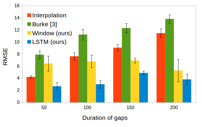
Figure 4. Dependency on the duration of the gap. Basketball motion. 5 missing markers.

Figure 4 shows that our methods can be applied for any length of gaps, while the performance of other methods degrades steadily with the increase of the length of the gap. Interpolation-based methods struggle to reconstruct markers when gaps become longer. Our method, in contrast, can propagate the information about the marker position using the hidden state, hence being robust to the long gaps.

6.3. Very long gaps

(a) Basketball: 3 markers missing

(b) Basketball: 30 markers missing

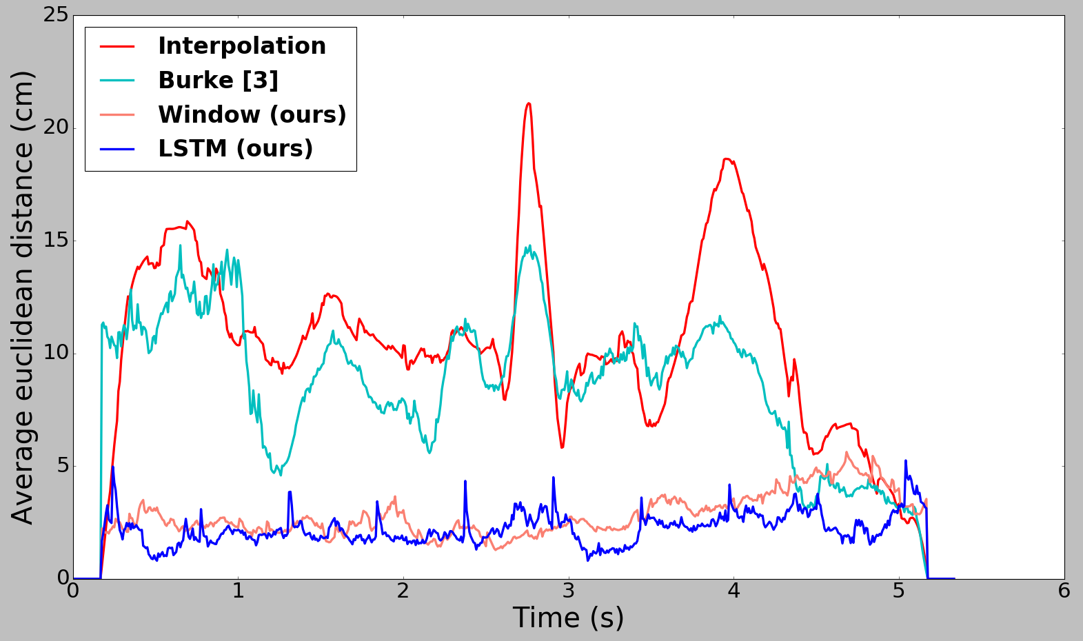
(c) Boxing: 3 markers missing

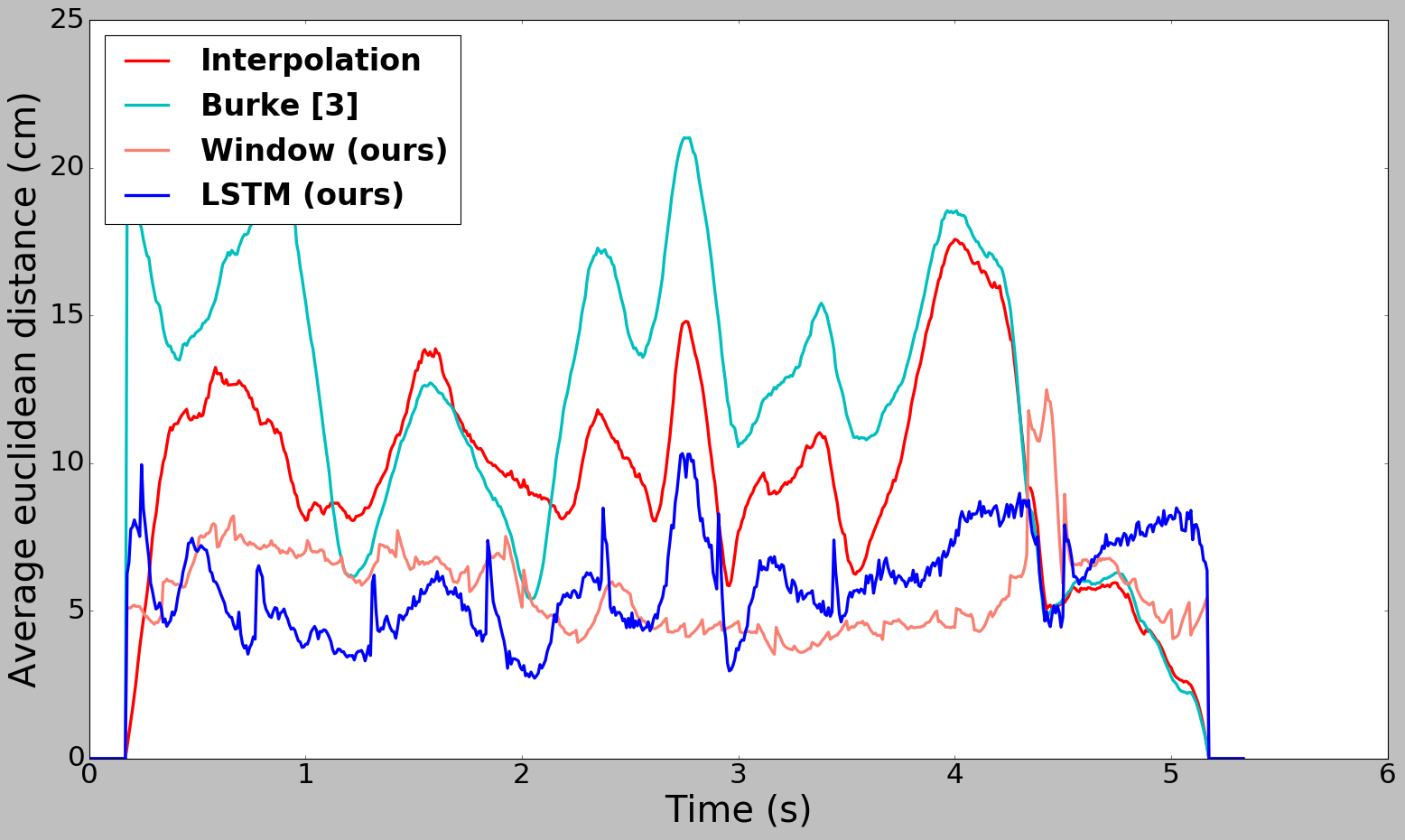
(d) Boxing: 30 markers missing

Figure 5. A few markers were missing over 5 seconds. All the markers were present for 1s before and after the gap.

In the following experiment, the same markers were missing over a long period of time. The measurement period started at 1.5 seconds into the clip to avoid artifacts. Then for 1 second, all markers were present, followed by a 5 second window where certain markers were missing for the entire time. Afterwards, all the markers were present again. Each experiment was repeated 5 times and the mean result was registered.

We can clearly see in Figure 5 that while interpolation and Burke(Burke and Lasenby, 2016) are quickly losing track of the markers, our methods stay stable and accurate. This hold for all the scenarios. Figure 5(b,d) illustrates that all methods except interpolation are degrading significantly when most of the markers are missing. That indicates that those methods are using information about the other markers, not only about the past or the future of a particular marker.

6.4. Visualization of the Results

Figure 6 illustrates the reconstruction results for one of the test sequences, boxing. The subject is boxing with their right arm. The observed marker cloud (Figure LABEL:fig:_VisualResultsb) misses 15 markers. Our reconstruction result (Figure LABEL:fig:_VisualResultsd) is visually close to the ground truth (Figure LABEL:fig:_VisualResultsa), which is also supported by the numerical errors.

6.5. Generalization

Table 3. Generalization test for the LSTM network. 20% of markers missing. Complete dataset contains motions from all the subjects and from all types. Then all motion with the same subject as in testing were removed. Finally all the recordings with the same type of motion very removed. Reconstruction error in cm is measured.

Motion / dataset	Basketball	Boxing
Complete	7.9 $\pm{0.14}$	2.08 $\pm{0.5}$
w/o the subject	9.93 $\pm{0.96}$	2.13 $\pm{0.42}$
w/o the motion	8.54 $\pm{1.04}$	2.57 $\pm{1.18}$

Table 4. Generalization test for the Window-based network. 20% of markers missing. The same setup as in Table 3.

Motion / dataset	Basketball	Boxing
Complete	5.59 $\pm{0.29}$	3.54 $\pm{0.15}$
w/o the subject	5.68 $\pm{0.48}$	4.37 $\pm{1.13}$
w/o the motion	6.52 $\pm{0.54}$	4.58 $\pm{1.51}$

Up to now, our models, as well as the baselines, have been trained with all motions and all individuals.

In the final experiments, we evaluated the generalization capability with respect to motion type and individual. To this end, we removed all the recordings of the test subject from the training data.Furthermore, for each test motion, we created a training set where this motion was removed. We then evaluated our networks while having 20% of the markers missing for gaps of 100 frames (almost 1 second).

Table 3 illustrates the results for the LSTM-based network and Table 4 for the Window-based method. We can observe that the performance drop is not dramatic: it is less than 25% and depends on the motion type and the network architecture. It is important to note that the variance is significantly higher for the ”generalization” scenarios, meaning that the system is less stable.

This experiment indicates that our systems can recover unseen motions, performed by unseen individuals, albeit with slightly worse performance.

7. Discussion and CONCLUSION

The experiments presented above show that the proposed methods can compensate for missing markers better than the state of the art, when the gap is long, especially when the motion is complex.

Our method is not relying on future frames, unlike most of the alternatives. That property makes it suitable for on-line usages when the markers are being reconstructed as they are collected.

Another notable property of the proposed method is that it can recover markers which are missing over a long period of time.

LSTM-based architecture is modeling the correlation is the human body to recover missing markers better than a window-based architecture, accordingly to our experiments.

In summary, the proposed methods can be used to recover markers over many frames in an accurate and stable way.

8. Acknowledgements

Authors would like to thank Simon Alexanderson and Judith Butepage for the useful discussions. This PhD project is supported by Swedish Foundation for Strategic Research Grant No.: RIT15-0107. The data used in this project was obtained from mocap.cs.cmu.edu. The database was created with funding from NSF EIA-0196217.

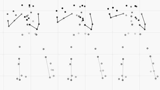
(a) Ground truth markers

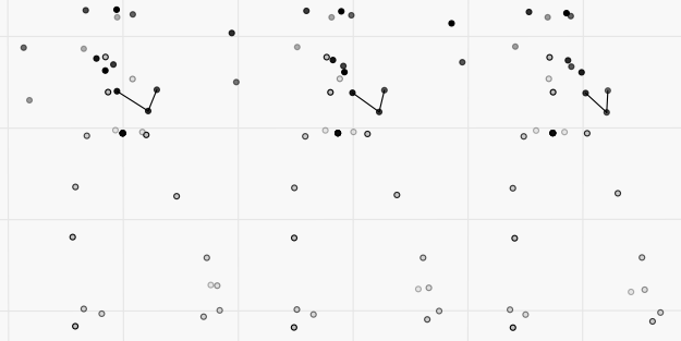
(b) 15 (our of 41) markers are missing

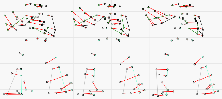
(c) Burke[3] reconstruction result

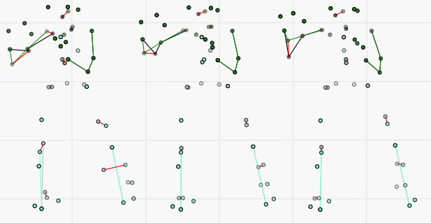
(d) LSTM (ours) reconstruction result

Figure 6. Three keyframes from the boxing test sequence, illustration of the reconstruction using the Burke and LSTM (ours) methods.

References

- (1)
- CMU (2003) 2003. Carnegie-Mellon Mocap Database. http://mocap.cs.cmu.edu/
- Abadi et al. (2016) Martín Abadi, Ashish Agarwal, Paul Barham, Eugene Brevdo, Zhifeng Chen, Craig Citro, Greg S Corrado, Andy Davis, Jeffrey Dean, Matthieu Devin, et al. 2016. Tensorflow: Large-scale machine learning on heterogeneous distributed systems. arXiv preprint arXiv:1603.04467 (2016).
- Burke and Lasenby (2016) Michael Burke and Joan Lasenby. 2016. Estimating missing marker positions using low dimensional Kalman smoothing. Journal of Biomechanics 49, 9 (2016), 1854–1858.
- Bütepage et al. (2017) Judith Bütepage, Michael Black, Danica Kragic, and Hedvig Kjellström. 2017. Deep representation learning for human motion prediction and classification. In IEEE Conference on Computer Vision and Pattern Recognition.
- Donahue et al. (2015) Jeffrey Donahue, Lisa Anne Hendricks, Sergio Guadarrama, Marcus Rohrbach, Subhashini Venugopalan, Kate Saenko, and Trevor Darrell. 2015. Long-term recurrent convolutional networks for visual recognition and description. In IEEE Conference on Computer Vision and Pattern Recognition.
- Fragkiadaki et al. (2015) Katerina Fragkiadaki, Sergey Levine, Panna Felsen, and Jitendra Malik. 2015. Recurrent network models for human dynamics. In IEEE International Conference on Computer Vision.
- Gløersen and Federolf (2016) Øyvind Gløersen and Peter Federolf. 2016. Predicting missing marker trajectories in human motion data using marker intercorrelations. PloS one 11, 3 (2016), e0152616.
- Hochreiter (1998) Sepp Hochreiter. 1998. The vanishing gradient problem during learning recurrent neural nets and problem solutions. International Journal of Uncertainty, Fuzziness and Knowledge-Based Systems 6, 2 (1998), 107–116.
- Hochreiter and Schmidhuber (1997) Sepp Hochreiter and Jürgen Schmidhuber. 1997. Long short-term memory. Neural Computation 9 (1997), 1735–1780.
- Holden (2018) Daniel Holden. 2018. Robust Solving of Optical Motion Capture Data by Denoising. ACM Trans. Graph. 38, 1 (2018).
- Hornik et al. (1989) Kurt Hornik, Maxwell Stinchcombe, and Halbert White. 1989. Multilayer feedforward networks are universal approximators. Neural networks 2, 5 (1989), 359–366.
- Jain et al. (2016) Ashesh Jain, Amir R Zamir, Silvio Savarese, and Ashutosh Saxena. 2016. Structural-RNN: Deep learning on spatio-temporal graphs. In IEEE Conference on Computer Vision and Pattern Recognition.
- Kingma and Ba (2014) Diederik Kingma and Jimmy Ba. 2014. Adam: A method for stochastic optimization. In International Conference on Learning Representations.
- Mall et al. (2017) Utkarsh Mall, G Roshan Lal, Siddhartha Chaudhuri, and Parag Chaudhuri. 2017. A deep recurrent framework for cleaning motion capture data. arXiv preprint arXiv:1712.03380 (2017).
- Peng et al. (2015) Shu-Juan Peng, Gao-Feng He, Xin Liu, and Hua-Zhen Wang. 2015. Hierarchical block-based incomplete human mocap data recovery using adaptive nonnegative matrix factorization. Computers & Graphics 49 (2015), 10–23.
- Shi et al. (2017) Baoguang Shi, Xiang Bai, and Cong Yao. 2017. An end-to-end trainable neural network for image-based sequence recognition and its application to scene text recognition. IEEE Transactions on Pattern Analysis and Machine Intelligence 39, 11 (2017), 2298–2304.
- Sutskever et al. (2014) Ilya Sutskever, Oriol Vinyals, and Quoc V Le. 2014. Sequence to sequence learning with neural networks. In Neural Information Processing Systems.
- Taylor et al. (2007) Graham W Taylor, Geoffrey E Hinton, and Sam T Roweis. 2007. Modeling human motion using binary latent variables. In Advances in neural information processing systems. 1345–1352.
- Vincent et al. (2008) Pascal Vincent, Hugo Larochelle, Yoshua Bengio, and Pierre-Antoine Manzagol. 2008. Extracting and composing robust features with denoising autoencoders. In International Conference on Machine Learning.
- Wang et al. (2016a) Zhao Wang, Yinfu Feng, Shuang Liu, Jun Xiao, Xiaosong Yang, and Jian J Zhang. 2016a. A 3D human motion refinement method based on sparse motion bases selection. In International Conference on Computer Animation and Social Agents.
- Wang et al. (2016b) Zhao Wang, Shuang Liu, Rongqiang Qian, Tao Jiang, Xiaosong Yang, and Jian J Zhang. 2016b. Human motion data refinement unitizing structural sparsity and spatial-temporal information. In IEEE Int. Conference on Signal Processing.