Borel Kernels and their Approximation, Categorically

Abstract.

This paper introduces a categorical framework to study the exact and approximate semantics of probabilistic programs. We construct a dagger symmetric monoidal category of Borel kernels where the dagger-structure is given by Bayesian inversion. We show functorial bridges between this category and categories of Banach lattices which formalize the move from kernel-based semantics to predicate transformer (backward) or state transformer (forward) semantics. These bridges are related by natural transformations, and we show in particular that the Radon-Nikodym and Riesz representation theorems - two pillars of probability theory - define natural transformations.

With the mathematical infrastructure in place, we present a generic and endogenous approach to approximating kernels on standard Borel spaces which exploits the involutive structure of our category of kernels. The approximation can be formulated in several equivalent ways by using the functorial bridges and natural transformations described above. Finally, we show that for sensible discretization schemes, every Borel kernel can be approximated by kernels on finite spaces, and that these approximations converge for a natural choice of topology.

We illustrate the theory by showing two examples of how approximation can effectively be used in practice: Bayesian inference and the Kleene $\ast$ operation of ProbNetKAT.

1. Introduction

Finding a good category in which to study probabilistic programs is a subject of active research (Staton et al., 2016; Kozen, 2016; Clerc et al., 2017; Staton, 2017). In this paper we present a dagger symmetric monoidal category of kernels whose dagger-structure is given by Bayesian inversion. The advantages of this new category are two-fold.

Firstly, the most important new construct introduced by probabilistic programming, viz. Bayesian inversion, is interpreted completely straightforwardly by the $\dagger$-operation which is native to our category. In particular we never leave the world of kernels and we therefore do not require any normalization construct. Consider for example the following simple Bayesian inference problem in Anglican ((Wood et al., 2014))

⬇

(defquery example

(let [x (sample (normal 0 1))]

(observe (normal x 1) 0.5)

(> x 1)))

The semantics of this program is build easily and compositionally in our category:

• The second line builds a Borel space equipped with a normally distributed probability measure – an object $(\mathbb{R},\mu)$ of our category.

• The (normal x 1) instruction builds a Borel kernel – a morphism $f:(\mathbb{R},\mu)\to(\mathbb{R},\nu)$ in our category.

• The observe statement builds the Bayesian inverse of the kernel – the morphism $f^{\dagger}:(\mathbb{R},\nu)\to(\mathbb{R},\mu)$ in our $\dagger$-category.

• Finally, the kernel $f^{\dagger}$ is evaluated, i.e. the denotation of the program above is $f^{\dagger}(0.5)(\left]1,\infty\right[)$.

The functoriality of $\dagger$ ensures compositionality.

Second, since Bayesian inference problems are in general very hard to compute (although the one given above has an analytical solution), it makes sense to seek approximate solutions, i.e. approximate denotations to probabilistic programs. As we will show, our category of kernels comes equipped with a generic and endogenous approximating scheme which relies on its involutive structure and on the structure of standard Borel spaces. Moreover, this approximation scheme can be shown to converge for any choice of kernel for a natural choice of topology.

Main contributions.

1. We build a category $\mathbf{Krn}$ of Borel kernels (§2) and we show how two kernels which agree almost everywhere can be identified under a categorical quotient operation. This technical construction is what allows us to define Bayesian inversion as an involutive functor, denoted $\dagger$. This is a key technical improvement on (Clerc et al., 2017) where the $\dagger$-structure was hinted at but was not functorial. We show that $\mathbf{Krn}$ is a dagger symmetric monoidal category.

2. We introduce the category $\mathbf{BL}_{\sigma}$ of Banach lattices and $\sigma$-order continuous positive operators as well as the Köthe dual functor $(-)^{\sigma}:\mathbf{BL}_{\sigma}^{\mathrm{op}}\to\mathbf{BL}_{\sigma}$ (§3). These will play a central role in studying convergence of our approximation schemes.

3. We provide the first categorical understanding of the Radon-Nikodym and the Riesz representation theorems. These arise as natural transformations between two functors relating kernels and Banach lattices (§4).

4. We show how the $\dagger$-structure of $\mathbf{Krn}$ can be exploited to approximate kernels by averaging (§5). Due to an important structural feature of $\mathbf{Krn}$ (Th. 1) every kernel in $\mathbf{Krn}$ can be approximated by kernels on finite spaces.

5. We show a natural class of approximations schemes where the sequence of approximating kernels converges to the kernel to be approximated. The notion of convergence is given naturally by moving to $\mathbf{BL}_{\sigma}$ and considering convergence in the Strong Operator Topology (§6).

6. We apply our theory of kernel approximations to two practical applications (§7). First, we show how Bayesian inference can be performed approximately by showing that the $\dagger$-operation commutes with taking approximations. Secondly, we consider the case of ProbNetKAT, a language developed in (Foster et al., 2016; Smolka et al., 2017) to probabilistically reason about networks. ProbNetKAT includes a Kleene star operator $(-)^{*}$ with a complex semantics which has proved hard to approximate. We show that $(-)^{*}$ can be approximated, and that the approximation converges.

All the proofs can be found in the Appendix.

Related work.

Quasi-Borel sets have recently been proposed as a semantic framework for higher-order probabilistic programs in (Staton et al., 2016). The main differences with our approach are: (i) unlike (Staton et al., 2016; Staton, 2017) we never leave the realm of kernels, and in particular we never need to worry about normalization. This makes the interpretation of observe statements, i.e. of Bayesian inversion, simpler and more natural. However, (ii) unlike the quasi-Borel sets of (Staton et al., 2016), our category is not Cartesian closed. We can therefore not give a semantics to all higher-order programs. This shortcoming is partly mitigated by the fact that the category of Polish space, on which our category ultimately rests, does have access to many function spaces, in particular all the spaces of functions whose domain is locally compact. We can thus in principle provide a semantics to higher-order programs, provided that $\lambda$-abstraction is restricted to locally compact spaces like the reals and the integers, although this won’t be investigated in this paper.

The approximation of probabilistic kernels has been a topic of investigation in theoretical computer science for nearly twenty years (see e.g. (Desharnais et al., 2000; Danos et al., 2003; Desharnais et al., 2004; Chaput et al., 2014)), and for much longer in the mathematical literature (e.g. (Choo-Whan, 1972)). Our results build on the formalism developed in (Chaput et al., 2014) with the following differences: (i) we can approximate kernels, their associated stochastic operator (backward predicate transformer), or their associated Markov operator (forward state transformer) with equivalent ease, and move freely across the three formalisms. (ii) Given a kernel $f:X\rightarrowtriangle Y$, we can define its approximation $f^{\prime}:X^{\prime}\to Y^{\prime}$ along any quotients $X^{\prime}$ of $X$ and $Y^{\prime}$ of $Y$ as in (Chaput et al., 2014), but we can also ‘internalize’ the approximation as a kernel $f^{*}:X\to Y$ of the original type. Morally $f^{\prime}$ and $f^{*}$ are the same approximation, but the second approximant, being of the same type as the original kernel, can be compared with it. In particular it becomes possible to study the convergence of ever finer approximations, which we do in Section 6. Finally, (iii) we opt to work with Banach lattices rather than the normed cones of (Selinger, 2004; Chaput et al., 2014) because it allows us to formulate the operator side of the theory very naturally, and it connects to a large body of classic mathematical results ((Aliprantis and Border, 1999; Zaanen, 2012)) which have been used in the semantics of probabilistic programs as far back as Kozen’s seminal (Kozen, 1981).

2. A category of Borel kernels

In (Clerc et al., 2017) the first three authors presented a category of Borel kernels similar in spirit to the construction of this section, but with a major shortcoming. As we will shortly see, our category $\mathbf{Krn}$ of Borel kernels can be equipped with an involutive functor – a dagger operation $\dagger$ in the terminology of (Selinger, 2007) – which captures the notion of Bayesian inversion and is absolutely crucial to everything that follows. In (Clerc et al., 2017) this operation had merely been identified as a map, i.e. not even as a functor. In this section we show that Bayesian inversion does indeed define a $\dagger$-structure on a more sophisticated – but measure-theoretically very natural – category of kernels.

2.1. Standard Borel spaces and the Giry monad

A standard Borel space – or SB space for short – is a measurable space $(X,\mathcal{S})$ for which there exists a Polish topology $\mathcal{T}$ on $X$ whose Borel sets are the elements of $\mathcal{S}$, i.e. such that $\mathcal{S}=\sigma(\mathcal{T})$ (see e.g. (Kechris, 1995) for an overview). Let us write $\mathbf{SB}$ for the category of standard Borel spaces and measurable maps. One key structural feature of $\mathbf{SB}$ is the following:

Theorem 1.

Every $\mathbf{SB}$ object is a limit of a countable co-directed diagram of finite spaces.

The Giry monad was originally defined in two variants (Giry, 1981): - As an endofunctor $\mathsf{G}_{\mathbf{Pol}}$ of $\mathbf{Pol}$, the category of Polish spaces, one sets $\mathsf{G}_{\mathbf{Pol}}(X,\mathcal{T})$ to be the space of Borel probability measures over $X$ together with the weak topology. This space is Polish (Kechris, 1995, Th 17.23), and the Portmanteau Theorem (Kechris, 1995, Th 17.20)) gives multiple characterizations of the weak topology. - As an endofunctor $\mathsf{G}_{\mathbf{Meas}}$ of $\mathbf{Meas}$, the category of measurable spaces, one sets $\mathsf{G}_{\mathbf{Meas}}(X,\mathcal{S})$ to be the set of probability measures on $X$ together with the initial $\sigma$-algebra for the maps $ev_{A}:\mathsf{G}_{\mathbf{Meas}}(X,\mathcal{S})\to\mathbb{R},\mu\mapsto\mu(A),A\in\mathcal{S}$.

In both cases the Giry monad is defined on an arrow $f:X\to Y$ as the map $f_{*}$ which sends a measure $\mu$ on $X$ to the pushforward measure $f_{*}\mu$ on $Y$, defined as $G(f)(\mu)(B)=f_{*}\mu(B):=\mu(f^{-1}(B))$ for $B$ a measurable subset of $Y$.

We want to define the Giry monad on the category $\mathbf{SB}$ of standard Borel spaces (and measurable maps), and the two versions of the Giry monad described above offer us natural ways to do this: given an SB space $(X,\sigma(\mathcal{T}))$ we can either compute $\mathsf{G}_{\mathbf{Pol}}(X,\mathcal{T})$ and take the associated standard Borel space, or directly compute $\mathsf{G}_{\mathbf{Meas}}(X,\sigma(\mathcal{T}))$. Fortunately, the two methods agree.

Theorem 2 ((Kechris, 1995), Th 17.24).

Let $\mathsf{B}:\mathbf{Pol}\to\mathbf{SB}$ denote the functor sending a Polish space $(X,\mathcal{T})$ to its associated SB-space $(X,\sigma(\mathcal{T}))$ and leaving morphisms unchanged, then

$$\mathsf{G}_{\mathbf{Meas}}\circ\mathsf{B}=\mathsf{B}\circ\mathsf{G}_{\mathbf{Pol}}.$$

We define the Giry monad on SB spaces to be the endofunctor $\mathsf{G}:\mathbf{SB}\to\mathbf{SB}$ defined by either of the two equivalent constructions above. The monadic data of $\mathsf{G}$ is given at each SB space $X$ by the unit $\delta_{X}:X\to\mathsf{G}X,x\mapsto\delta_{x}$, the Dirac $\delta$ measure at $x$, and the multiplication $m_{X}:\mathsf{G}^{2}X\to\mathsf{G}X,\mathbb{P}\mapsto\lambda A.\int_{\mathsf{G}X}ev_{A}d\mathbb{P}$. We refer the reader to (Giry, 1981) for proofs that $\delta_{X}$ and $m_{X}$ are measurable.

2.2. The construction of $\mathbf{Krn}$

Let us denote by ${\mathbf{SB}_{\mathsf{G}}}$ the Kleisli category associated with the Giry monad $(\mathsf{G},\delta,m)$. We denote Kleisli arrows, i.e. Markov kernels, by $X\rightarrowtriangle Y$, and we call such an arrow deterministic if it can be factorized as an ordinary measurable function followed by the unit $\delta$. Kleisli composition is denoted by $\bullet$. The category $\ast\downarrow{\mathbf{SB}_{\mathsf{G}}}$ has arrows $\ast\rightarrowtriangle X$ as objects, where $\ast$ is the one point SB space (the terminal object in $\mathbf{SB}$). An arrow from $\mu:\ast\rightarrowtriangle X$ to $\nu:\ast\rightarrowtriangle Y$ is a ${\mathbf{SB}_{\mathsf{G}}}$ arrow $f:X\rightarrowtriangle Y$ such that $\nu=f\bullet\mu$, i.e. such that $\nu(A)=\int_{X}f(x)(A)d\mu$ for any measurable subset $A$ of $Y$. This situation will be denoted in short by $f:(X,\mu)\rightarrowtriangle(Y,\nu)$, and we will call a pair $(X,\mu)$ a measured SB space.

We want to construct a quotient of $\ast\downarrow{\mathbf{SB}_{\mathsf{G}}}$, such that two $\ast\downarrow{\mathbf{SB}_{\mathsf{G}}}$ arrows are identified if they disagree on a null set w.r.t. the measure on their domain. For $g,g^{\prime}:(X,\mu)\rightarrowtriangle(Y,\nu)$, we define $N(g,g^{\prime})=\{x\in X\mid g(x)\neq g^{\prime}(x)\}$.

Lemma 3.

$N(g,g^{\prime})$ is a measurable set.

We now define a relation $\sim$ on $\mathrm{Hom}((X,\mu),(Y,\nu))$ by saying that for any two arrows $g,g^{\prime}:(X,\mu)\rightarrowtriangle(Y,\nu)$, $g\sim g^{\prime}\text{ if }\mu(N(g,g^{\prime}))=0$. This clearly defines an equivalence relation on $\mathrm{Hom}((X,\mu),(Y,\nu))$. In order to perform the quotient of the category $\ast\downarrow{\mathbf{SB}_{\mathsf{G}}}$ modulo $\sim$, we need to check that it is compatible with composition.

Proposition 4.

If $g\sim g^{\prime}$, then $h\bullet g\bullet f\sim h\bullet g^{\prime}\bullet f$.

Definition 5.

Let $\mathbf{Krn}$ be the category obtained by quotienting $\ast\downarrow{\mathbf{SB}_{\mathsf{G}}}$ hom-sets with $\sim$.

The following Theorem is of great practical use and generalizes the well-known result for deterministic arrows.

Theorem 6 (Change of Variables in $\mathbf{Krn}$).

Let $f:(X,\mu)\rightarrowtriangle(Y,\nu)$ be a $\mathbf{Krn}$-morphism. For any measurable function $\phi:Y\to\mathbb{R}$, if $\phi$ is $\nu$-integrable, then $\phi\bullet f(x)=\int_{Y}\phi\,df(x)$ is $\mu$-integrable and

$$\int_{Y}\phi~{}d\nu=\int_{X}\phi\bullet f~{}d\mu$$

The symmetric monoidal structure of $\hskip 2.0pt\mathbf{Krn}$

is defined on a pair of objects $(X,\mu),(Y,\nu)$ by the Cartesian product and the product of measure, i.e. $(X,\mu)\otimes(Y,\nu)=(X\times Y,\mu\otimes\nu)$. On pairs of morphisms $f:(X,\mu)\rightarrowtriangle(Y,\nu)$ and $f^{\prime}:(X^{\prime},\mu^{\prime})\rightarrowtriangle(Y^{\prime},\nu^{\prime})$ it is defined by $(f\otimes f^{\prime})(x,x^{\prime}):=f(x)\otimes f^{\prime}(x^{\prime})$. The unitors, associator and braiding transformations are given by the obvious bijections.

2.3. The dagger structure of $\mathbf{Krn}$

$\mathbf{Krn}$ has an extremely powerful inversion principle:

Theorem 7 (Measure Disintegration Theorem, (Kechris, 1995), 17.35).

Let $f:(X,\mu)\rightarrowtriangle(Y,\nu)$ be a deterministic $\mathbf{Krn}$-morphism, there exists a unique morphism $f^{\dagger}_{\mu}:(Y,\nu)\rightarrowtriangle(X,\mu)$ such that

(1) $$f\bullet f^{\dagger}_{\mu}=\mathrm{id}_{(Y,\nu)}.$$

The kernel $f^{\dagger}_{\mu}$ is called the disintegration of $\mu$ along $f$. As our notation suggests, the disintegration depends fundamentally on the measure $\mu$ over the domain, however we will omit this subscript when there is no ambiguity. The following lemma relates disintegrations to conditional expectations.

Lemma 8 ((Dahlqvist et al., 2016b)).

Let $f:(X,\mu)\to(Y,\nu)$ be a deterministic $\mathbf{Krn}$-morphism, and let $\phi:X\to\mathbb{R}$ be measurable, then $\mu$-a.e.

$$\phi\bullet f^{\dagger}\bullet f=\mathbb{E}\left[\phi\mid\sigma(f)\right]$$

We can extend the definition of $(-)^{\dagger}$ to any $\mathbf{Krn}$-morphism $f:(X,\mu)\rightarrowtriangle(Y,\nu)$ in a functorial way, although $f^{\dagger}$ will not in general be a right inverse to $f$. The construction of $f^{\dagger}$ is detailed in (Clerc et al., 2017), but let us briefly recall how it works. The category $\mathbf{SB}$ has products which are built in the same way as in $\mathbf{Meas}$ via the product of $\sigma$-algebras. Given any kernel $f:(X,\mu)\rightarrowtriangle(Y,\nu)$, we can canonically construct a probability measure $\gamma_{f}$ on the product $X\times Y$ of SB-space by defining it on the rectangles of $X\times Y$ as

(2) $$\gamma_{f}(A\times B)=\int_{x\in X}1_{A}(x)\cdot f(x)(B)~{}d\mu.$$

Equivalently, $\gamma_{f}=(\delta_{X}\otimes f)\bullet\Delta_{X}\bullet\mu$, where $\Delta_{X}:X\to X\times X$ is the diagonal map. Letting $\pi_{X}:X\times Y\to X$ and $\pi_{Y}:X\times Y\to Y$ be the canonical projections, we observe that $\mathsf{G}\pi_{X}(\gamma_{f})=\mu$ and $\mathsf{G}\pi_{Y}(\gamma_{f})=\nu$: in other words, $\gamma_{f}$ is a coupling of $\mu$ and $\nu$. The disintegration of $\gamma_{f}$ along $\pi_{Y}$ is a kernel $\pi_{Y}^{\dagger}:(Y,\nu)\to(X\times Y,\gamma_{f})$. Finally we define:

(3) $$f^{\dagger}=\pi_{X}\bullet\pi_{Y}^{\dagger}.$$

The following $\mathbf{Krn}$ diagram sums up the situation:

where $\pi^{\dagger}_{X}$ is explicitly given by $(\delta_{X}\otimes f)\bullet\Delta_{X}$. The following property characterizes the action of $(-)^{\dagger}$ on $\mathbf{Krn}$-morphisms:

Theorem 9.

For all $f:(X,\mu)\rightarrowtriangle(Y,\nu)$, $f^{\dagger}:(Y,\nu)\rightarrowtriangle(X,\mu)$ is the unique $\mathbf{Krn}$ morphism satisfying for all measurable sets $A\subseteq X$, $B\subseteq Y$ the following equation:

(4) $$\int_{x\in X}1_{A}(x)\cdot f(x)(B)~{}d\mu=\int_{y\in Y}f^{\dagger}(y)(A)\cdot 1_{B}(y)~{}d\nu$$

In view of Eq. (4), we will call $f^{\dagger}$ the Bayesian inversion of $f$, and refer to $(-)^{\dagger}$ as the Bayesian inversion operation on $\mathbf{Krn}$. It will be crucial throughout the rest of this paper. It is important to see that $f^{\dagger}$ absolutely depends on the choice of $\mu$ and not only on $f$ seen as a function. We can now improve on (Clerc et al., 2017) and show that $(-)^{\dagger}$ is indeed a $\dagger$-operation in the strict categorical meaning of the term.

Theorem 10.

$\mathbf{Krn}$ is a dagger symmetric monoidal category, with $(-)^{\dagger}$ given by Bayesian inversion.

3. Banach lattices

It is well-known that kernels can alternatively be seen as predicate – i.e. real-valued function –transformers, or as state – i.e. probability measure – transformers. The latter perspective was adopted by Kozen in (Kozen, 1981) to describe the denotational semantics of probabilistic programs (without conditioning). We shall see in this section and the next, that the predicate and state transformer perspectives are dual to one another in the category of Banach lattices, a framework incidentally also used in (Kozen, 1981). For an introduction to the theory of Banach lattices we refer the reader to e.g. (Aliprantis and Border, 1999; Zaanen, 2012).

An ordered real vector space $V$ is a real vector space together with a partial order $\leq$ which is compatible with the linear structure in the sense that for all $u,v,w\in V,\lambda\in\mathbb{R}^{+}$

$$u\leq v\Rightarrow u+w\leq v+w\qquad\text{and}\qquad u\leq v\Rightarrow\lambda u\leq\lambda v$$

An ordered vector space $(V,\leq)$ is called a Riesz space if the poset structure forms a lattice. A vector $v$ in a Riesz space $(V,\leq)$ is called positive if $0\leq v$, and its absolute value $\left|v\right|$ is defined as $\left|v\right|=v\vee(-v)$. A Riesz space $(V,\leq)$ is $\sigma$-order complete if every non-empty countable subset of $V$ which is order bounded has a supremum.

A normed Riesz space is a Riesz space $(V,\leq)$ equipped with a lattice norm, i.e. a map $\left\lVert\cdot\right\rVert:V\to\mathbb{R}$ such that:

(5) $$\left|v\right|\leq\left|w\right|\text{ implies }\left\lVert v\right\rVert\leq\left\lVert w\right\rVert.$$

A normed Riesz space is called a Banach lattice if it is (norm-) complete, i.e. if every Cauchy sequence (for the norm $\left\lVert\cdot\right\rVert$) has a limit in $V$.

Example 1.

For each measured space $(X,\mu)$ – and in particular $\mathbf{Krn}$-objects – and each $1\leq p\leq\infty$, the space $\mathrm{L}_{p}(X,\mu)$ is a Riesz space with the pointwise order. When it is equipped with the usual $\mathrm{L}_{p}$-norm, it is a Banach lattice. This fact is often referred to as the Riesz-Fischer theorem (see (Aliprantis and Border, 1999, Th 13.5)). We will say that $p,q\in\mathbb{N}\cup\{\infty\}$ are Hölder conjugate if either of the following conditions hold: (i) $1<p,q<\infty$ and $\frac{1}{p}+\frac{1}{q}=1$, or (ii) $p=1$ and $q=\infty$, or (iii) $p=\infty$ and $q=1$.

Theorem 2 (Lemma 16.1 and Theorem 16.2 of (Zaanen, 2012)).

Every Banach lattice is $\sigma$-order complete.

There are two very natural modes of ‘convergence’ in a Banach lattice: order convergence and norm convergence. The latter is well-known, the former less so. An order bounded sequence $\{v_{n}\}_{n\in\mathbb{N}}$ in a $\sigma$-complete Riesz space (and thus in a Banach lattice) converges in order to $v$ if either of the following equivalent conditions holds:

$$v=\liminf_{n}v_{n}:=\bigvee_{n}\bigwedge_{n\leq m}v_{m},\hskip 10.00002ptv=\limsup_{n}v_{n}:=\bigwedge_{n}\bigvee_{n\leq m}v_{m}.$$

For a monotone increasing sequence $v_{n}$, this definition simplifies to $v=\bigvee_{n}v_{n}$, which is often written $v_{n}\uparrow v$.

In a general $\sigma$-complete Riesz space, order and norm convergence are disjoint concepts, i.e. neither implies the other (see (Zaanen, 2012, Ex. 15.2) for two counter-examples). However if a sequence converges both in order and in norm then the limits are the same (see (Zaanen, 2012, Th. 15.4)). Moreover, for monotone sequences norm convergence implies order convergence:

Proposition 3 ((Zaanen, 2012) Theorem 15.3).

If $\{v_{n}\}_{n\in\mathbb{N}}$ is an increasing sequence in a normed Riesz space and if $v_{n}$ converges to $v$ in norm (notation $v_{n}\to v)$, then $v_{n}\uparrow v$.

In a Banach lattice we have the following stronger property.

Proposition 4 (Lemma 16.1 and Theorem 16.2 of (Zaanen, 2012)).

If $\{v_{n}\}_{n\in\mathbb{N}}$ is a sequence of positive vectors in a Banach lattice such that $\sup_{n}\left\lVert v_{n}\right\rVert$ converges, then $\bigvee_{n}v_{n}$ exists and $\left\lVert\bigvee_{n}v_{n}\right\rVert=\bigvee_{n}\left\lVert v_{n}\right\rVert$.

It can also happen that order convergence implies norm convergence. A lattice norm on a Riesz space is called $\sigma$-order continuous if $v_{n}\downarrow 0$ ($v_{n}$ is a decreasing sequence whose infimum is 0) implies $\left\lVert v_{n}\right\rVert\downarrow 0$.

Example 5.

For $1\leq p<\infty$, the $\mathrm{L}_{p}$-norm is $\sigma$-order continuous, and thus order convergence and norm convergence coincide. However, for $p=\infty$ this is not the case as the following simple example shows. Consider the sequence of essentially bounded functions $v_{n}=1_{[n,+\infty[}$: it is decreasing for the order on $\mathrm{L}_{\infty}(\mathbb{R},\lambda)$ with the constant function $0$ as its infimum, i.e. $v_{n}\downarrow 0$. However $\left\lVert v_{n}\right\rVert=1$ for all $n$.

Many types of morphisms between Banach lattices are considered in the literature but most are at least linear and positive, that is to say they send positive vectors to positive vectors. From now on, we will assume that all morphisms are positive (linear) operators. Other than that, we will only mention two additional properties, corresponding to the two modes of convergence which we have examined. The first notion is very well-known: a linear operator $T:V\to W$ between normed vector spaces is called norm-bounded if there exists $C\in\mathbb{R}$ such that $\left\lVert Tv\right\rVert\leq C\left\lVert v\right\rVert$ for every $v\in V$. The following result is familiar:

Theorem 6.

An operator $T:V\to W$ between normed vector spaces is norm-bounded iff it is continuous.

Thus norm-bounded operators preserve norm-convergence. The corresponding order-convergence concept is defined as follows: an operator $T:V\to W$ between $\sigma$-order complete Riesz spaces is said to be $\sigma$-order continuous if whenever $v_{n}\uparrow v$, $Tv=\bigvee Tv_{n}$. It follows that we can consider two types of dual spaces on a Banach lattice $V$: on the one hand we can consider the norm-dual:

$$V^{*}=\{f:V\to\mathbb{R}\mid f\text{ is norm-continuous}\}$$

and the $\sigma$-order-dual:

$$V^{\sigma}=\{f:V\to\mathbb{R}\mid f\text{ is $\sigma$-order continuous}\}$$

The latter is sometimes known as the Köthe dual of $V$ (see (Dieudonné, 1951; Zaanen, 2012)). The two types of duals coincide for a large class of Banach spaces of interest to us.

Theorem 7.

If a Banach lattice $V$ admits a strictly positive linear functional and has a $\sigma$-order-continuous norm, then $V^{*}=V^{\sigma}$.

Example 8.

The result above can directly be applied to our running example: given a measured space $(X,\mu)$ and an integer $1\leq p<\infty$, the Lebesgue integral provides a strictly positive functional on $\mathrm{L}_{p}(X,\mu)$, and we already know from Example 5 that $\mathrm{L}_{p}(X,\mu)$ has a $\sigma$-order-continuous norm. It follows that

$$\mathrm{L}_{p}(X,\mu)^{*}=\mathrm{L}_{p}(X,\mu)^{\sigma}$$

Moreover, it is well-known that if $(p,q)$ are Hölder conjugate and $1<p,q<\infty$, then $\mathrm{L}_{p}(X,\mu)^{*}=\mathrm{L}_{q}(X,\mu)$, and thus $\mathrm{L}_{p}(X,\mu)^{\sigma}=\mathrm{L}_{q}(X,\mu)$. It is also known that $\mathrm{L}_{1}(X,\mu)^{*}=\mathrm{L}_{\infty}(X,\mu)$, and thus $\mathrm{L}_{1}(X,\mu)^{\sigma}=\mathrm{L}_{\infty}(X,\mu)$.

However Theorem 7 does not hold for $\mathrm{L}_{\infty}(X,\mu)$ since the $\mathrm{L}_{\infty}$-norm is not $\sigma$-order continuous, as was shown in Example 5. It is well-known that $\mathrm{L}_{\infty}(X,\mu)^{*}\neq\mathrm{L}_{1}(X,\mu)$, and in fact $\mathrm{L}_{\infty}(X,\mu)^{*}$ can be concretely described as the Banach lattice $\mathrm{ba}(X,\mu)$ of charges (i.e. finitely additive finite signed measures) which are absolutely continuous w.r.t, $\mu$ on $X$ (see (Dunford et al., 1971, IV.8.16)). However, as is shown in e.g. (Zaanen, 2012; Chaput et al., 2014)

(6) $$\mathrm{L}_{\infty}(X,\mu)^{\sigma}=\mathrm{L}_{1}(X,\mu)$$

As Examples 5 and 8 show, the $(-)^{\sigma}$ operation brings a lot of symmetry to the relationship between $\mathrm{L}_{p}$-spaces since

$$\mathrm{L}_{p}(X,\mu)^{\sigma}=\mathrm{L}_{q}(X,\mu)$$

for any Hölder conjugate pair $1\leq p\leq\infty$. For this reason we will consider the category $\mathbf{BL}_{\sigma}$ whose objects are Banach lattices and whose morphisms are $\sigma$-order continuous positive operators. Note that the Köthe dual of a Banach lattice is a Banach lattice, and it easily follows that $(-)^{\sigma}$ in fact defines a contravariant functor $\mathbf{BL}_{\sigma}^{\mathrm{op}}\to\mathbf{BL}_{\sigma}$ which acts on morphisms by pre-composition. As we will now see, $\mathbf{BL}_{\sigma}$ is the category in which predicate and state transformers are most naturally defined.

4. From Borel kernels to Banach lattices

The functors $\mathsf{S}_{p}$ and $\mathsf{T}_{p}$.

For $1\leq p\leq\infty$, the operation which associates to a $\mathbf{Krn}$-object $(X,\mu)$ the space $\mathrm{L}_{p}(X,\mu)$ can be thought of as either a contravariant or a covariant functor. We define the functors $\mathsf{S}_{p}:\mathbf{Krn}\to\mathbf{BL}_{\sigma}^{\mathrm{op}},1\leq p\leq\infty$ as expected on objects, and on $\mathbf{Krn}$-morphisms $f:X\rightarrowtriangle Y$ via the well-known ‘predicate transformer’ perspective:

$$\mathsf{S}_{p}(f):\mathrm{L}_{p}(Y,\nu)\to\mathrm{L}_{p}(X,\mu),\phi\mapsto\lambda x.\int_{Y}\phi\,df(x)=\phi\bullet f$$

For a proof that this defines a functor see (Clerc et al., 2017). We define the covariant functors $\mathsf{T}_{p}:\mathbf{Krn}\to\mathbf{BL}_{\sigma},1\leq p\leq\infty$ as $\mathsf{T}_{p}=\mathsf{S}_{p}\circ(-)^{\dagger}$.

The functor $\mathcal{M}^{\ll\cdot}$.

An ideal of a Riesz space $V$ is a sub-vector space $U\subseteq V$ with the property that if $\left|u\right|\leq\left|v\right|$ and $v\in U$ then $u\in U$. An ideal $U$ is called a band when for every subset $D\subseteq U$ if $\bigvee D$ exists in $V$, then it also belongs to $U$. Every band in a Banach lattice is itself a Banach lattice. Of particular importance is the band $B_{v}$ generated by a singleton $\{v\}$, which can be described explicitly as

$$B_{v}=\{w\in V\mid(\left|w\right|\wedge n\left|v\right|)\uparrow\left|w\right|\}$$

Example 1.

Let $X$ be an SB-space and $\mathsf{ca}(X)$ denote the set of measures of bounded variation on $X$. It can be shown ((Aliprantis and Border, 1999, Th 10.56)) that $\mathsf{ca}(X)$ is a Banach lattice. The linear structure on $\mathsf{ca}(X)$ is as expected, the Riesz space structure is given by

$$(\mu\vee\nu)(A)=\sup\{\mu(B)+\nu(A\setminus B)\mid B\text{ measurable },B\subseteq A\}$$

and the dual definition for the meet operation. The norm is given by the total variation i.e.

$$\left\lVert\mu\right\rVert=\sup\left\{\sum_{i}^{n}\left|\mu(A_{i})\right|\bigg{|}\{A_{1},\ldots,A_{n}\}\text{ a meas. partition of }X\right\}$$

Given $\mu\in\mathsf{ca}(X)$, the band $B_{\mu}$ generated by $\mu$ is just the set of measures of bounded variation which are absolutely continuous w.r.t. $\mu$. In particular $B_{\mu}$ is a Banach lattice.

We can now define the functor $\mathcal{M}^{\ll\cdot}:\mathbf{Krn}\to\mathbf{BL}_{\sigma}$ by:

$$\begin{cases}\mathcal{M}^{\ll\cdot}(X,\mu):=B_{\mu}\\ \mathcal{M}^{\ll\cdot}f:\mathcal{M}^{\ll\cdot}(X,\mu)\to\mathcal{M}^{\ll\cdot}(Y,\nu),\rho\mapsto f\bullet\rho\end{cases}$$

We will usually write $\mathcal{M}^{\ll\cdot}(X,\mu)$ as $\mathcal{M}^{\ll\mu}(X)$.

Proposition 2.

Let $f:(X,\mu)\rightarrowtriangle(Y,\nu)$ be a $\mathbf{Krn}$ arrow. Let $\rho$ be a finite measure on $X$ such that $\rho\ll\mu$. Then $f\bullet\rho\ll\nu$, and thus $\mathcal{M}^{\ll\cdot}$ defines a functor.

Radon-Nikodym is natural.

We now present a first pair of natural transformations which will establish a natural isomorphism between the functors $\mathsf{T}_{1}$ and $\mathcal{M}^{\ll\cdot}$. First, we define the Radon-Nikodym transformation $\mathsf{rn}:\mathcal{M}^{\ll\cdot}\to\mathsf{T}_{1}$ at each $\mathbf{Krn}$-object $(X,\mu)$ by the map

$$\mathsf{rn}_{(X,\mu)}:\mathcal{M}^{\ll\mu}(X)\to\mathrm{L}_{1}(X,\mu),\quad\mathsf{rn}_{(X,\mu)}(\rho)=\frac{d\rho}{d\mu}$$

where $\nicefrac{{d\rho}}{{d\mu}}$ is of course the Radon-Nikodym derivative of $\rho$ w.r.t. $\mu$. The fact that this transformation defines a positive operator between Banach lattices is simply a restatement of the usual Radon-Nikodym theorem (Dunford et al., 1971, III.10.7.), combined with the well-known linearity property of the Radon-Nikodym derivative. To see that it is also $\sigma$-order-continuous, consider a monotone sequence $\mu_{n}\uparrow\mu$ converging in order to $\mu$ in $\mathcal{M}^{\ll\nu}(X)$. This means that for any measurable set $A$ of $X$, $\lim_{n\to\infty}\mu_{n}(A)=\mu(A)$. Since $(\nicefrac{{d\mu_{n}}}{{d\nu}})_{n\in\mathbb{N}}$ is bounded in $\mathrm{L}_{1}$-norm the function $g=\bigvee_{n}\nicefrac{{d\mu_{n}}}{{d\nu}}$ exists and is simply the pointwise limit $g(x)=\lim_{n\to\infty}\nicefrac{{d\mu_{n}}}{{d\nu}}(x)$. It now follows from the monotone convergence theorem (MCT) that

$$\int_{A}gd\nu=\int_{A}\lim_{n\to\infty}\frac{d\mu_{n}}{d\nu}d\nu=\lim_{n\to\infty}\int_{A}\frac{d\mu_{n}}{d\nu}d\nu=\lim_{n\to\infty}\mu_{n}(A)=\mu(A)$$

in other words, $g=\nicefrac{{d\mu}}{{d\nu}}$ and $\mathsf{rn}$ is well-defined. That $\mathsf{rn}$ is also natural has – to our knowledge – never been published.

Theorem 3.

The Radon-Nikodym transformation is natural.

Secondly, we define the Measure Representation transformation $\mathsf{mr}:\mathsf{T}_{1}\to\mathcal{M}^{\ll\cdot}$ at each $\mathbf{Krn}$-object $(X,\mu)$ by the map $\mathsf{mr}_{(X,\mu)}:\mathsf{T}_{1}(X,\mu)\to\mathcal{M}^{\ll\cdot}(X,\mu)$ defined as

$$\mathsf{mr}_{(X,\mu)}(f)(B_{X})=\int_{B_{X}}fd\mu$$

This is a very well-known construction in measure theory, and the fact that $\mathsf{mr}_{(X,\mu)}$ is a $\sigma$-order continuous operator between Banach lattices is immediate from the linearity of integrals and the MCT.

Theorem 4.

The Measure Representation transformation is natural.

Riesz representations are natural.

We now present a second pair of natural transformations which will establish a natural isomorphism between $(-)^{\sigma}\circ\mathsf{S}_{\infty}$ and $\mathcal{M}^{\ll\cdot}$. First, we define the Riesz Representation transformation $\mathsf{rr}:(-)^{\sigma}\circ\mathsf{S}_{\infty}\to\mathcal{M}^{\ll\cdot}$ at each $\mathbf{Krn}$-object $(X,\mu)$ by the map $\mathsf{rr}_{(X,\mu)}:(-)^{\sigma}\circ\mathsf{S}_{\infty}(X,\mu)\to\mathcal{M}^{\ll\cdot}(X,\mu)$ defined as

$$\mathsf{rr}_{(X,\mu)}(F)(B_{X})=F(1_{B_{X}})$$

This construction is key to a whole collection of results in functional analysis commonly known as Riesz Representation Theorems (see (Aliprantis and Border, 1999) Chapter 14 for an overview). One can readily check that the Riesz Representation transformation is well-defined: $\mathsf{rr}_{(X,\mu)}(F)(\emptyset)=F(0)=0$ and the $\sigma$-additivity of $\mathsf{rr}_{(X,\mu)}(F)$ follows from the $\sigma$-order-continuity of $F$. To see that $\mathsf{rr}_{(X,\mu)}(F)\ll\mu$, assume that $\mu(B_{X})=0$, then clearly $1_{B_{X}}=0$ $\mu$-a.e., i.e. $1_{B_{X}}=0$ in $\mathrm{L}_{\infty}(X,\mu)$, and thus $F(1_{B_{X}})=0$.

Theorem 5.

The Riesz Representation transformation is natural.

Finally, we define the Functional Representation transformation $\mathsf{fr}$ at each $\mathbf{Krn}$-object $(X,\mu)$ by the map $\mathsf{fr}_{(X,\mu)}:\mathcal{M}^{\ll\cdot}(X,\mu)\to(-)^{\sigma}\circ\mathsf{S}_{\infty}(X,\mu)$ by

$$\mathsf{fr}_{(X,\mu)}(\mu)(\phi)=\int_{X}\phi d\mu$$

This construction is also completely standard in measure theory, although it has never to our knowledge been seen as a natural transformation.

Theorem 6.

The Functional Representation transformation is well-defined, i.e. $\mathsf{fr}_{(X,\mu)}$ is a $\sigma$-order continuous positive operator, and is natural.

Natural Isomorphisms

We have now defined the following four natural transformations:

In fact, both pairs form natural isomorphisms, and these can be restricted to arbitrary Hölder conjugate pairs $(p,q)$.

Theorem 7.

$\mathsf{rn}$ and $\mathsf{mr}$ are inverse of one another, in particular there exists a natural isomorphism between $\mathcal{M}^{\ll\mu}(X)$ and $\mathrm{L}_{1}(X,\mu)$.

Theorem 8.

$\mathsf{rr}$ and $\mathsf{fr}$ are inverse of each other, in particular there exists a natural isomorphism between $\mathcal{M}^{\ll\mu}(X)$ and $(\mathrm{L}_{\infty}(X,\mu))^{\sigma}$.

We can now conclude that the isomorphism proved in Theorem 6 of (Clerc et al., 2017) is in fact natural.

Corollary 9.

There exists a natural isomorphism between $\mathsf{T}_{1}:=\mathsf{S}_{1}\circ(-)^{\dagger}$ and $(-)^{\sigma}\circ\mathsf{S}_{\infty}$.

We can in fact restrict this result to any Hölder conjugate pair $(p,q)$:

Theorem 10.

For $1\leq p\leq\infty$ with Hölder conjugate $q$, the natural transformation $\mathsf{rn}\circ\mathsf{rr}$ restricts to a natural transformation $(-)^{\sigma}\circ\mathsf{S}_{q}\to\mathsf{T}_{p}$.

The correspondence between the various categories and functors discussed in this section are summarized as follows:

(7)

5. Approximations

In this section we develop a scheme for approximating kernels which follows naturally from the $\dagger$-structure of $\mathbf{Krn}$. Consider $f:(X,\mu)\rightarrowtriangle(Y,\nu)$ and a pair of deterministic maps $p:(X,\mu)\to(X^{\prime},p_{\ast}\mu)$ and $q:(Y,\nu)\to(Y^{\prime},q_{\ast}\nu)$ (typically these maps coarsen the spaces $X$ and $Y$).

(8)

The $\dagger$-structure of $\mathbf{Krn}$ allows us to define the new kernels

(9) $$f^{p,q}:=q^{\dagger}_{\nu}\bullet q\bullet f\bullet p^{\dagger}_{\mu}\bullet p :X\hskip 3.0pt\rightarrowtriangle Y\hskip 3.0pt$$

(10) $$f_{p,q}:=q\bullet f\bullet p^{\dagger}_{\mu} :X^{\prime}\rightarrowtriangle Y^{\prime}$$

The supscript notation is meant to indicate that the approximation lives ‘upstairs’ in Diagram (8) and conversely for the subscripts. Intuitively, $f_{p,q}$ and $f^{p,q}$ take the average of $f$ over the fibres given by $p,q$ according to $\mu$ and $\nu$ (see Section 7 for concrete calculations). The advantage of (10) is that we can approximate a kernel on a huge space by a kernel on a, say, finite one. The advantage of (9) is that although it is more complicated, it is morally equivalent and has the same type as $f$, which means that we can compare it to $f$.

A very simple consequence of our definition is that Bayesian inversion commutes with approximations. We shall use this in §7.1 to perform approximate Bayesian inference.

Theorem 1.

Let $f:(X,\mu)\rightarrowtriangle(Y,\nu)$, let $p:X\to X^{\prime}$ and $q:Y\to Y^{\prime}n$ be a pair of deterministic maps, then

$$(f^{\dagger})^{q,p}=(f^{p,q})^{\dagger}\text{ and }(f^{\dagger})_{q,p}=(f_{p,q})^{\dagger}$$

In practice we will often consider endo-kernels $f:X\rightarrowtriangle X$ with a single coarsening map $p:X\to X^{\prime}$ to a finite space. In this case (9) simplifies greatly.

Proposition 2.

Under the situation described above

(11) $$f^{p}:=p^{\dagger}_{\nu}\bullet p\bullet f\bullet p^{\dagger}_{\mu}\bullet p=f\bullet p^{\dagger}_{\mu}\bullet p$$

In the case covered by Proposition 2, the interpretation of $f^{p}$ is very natural: for each $x\in X$ the measure $f(x)$ is approximated by its average over the fibre to which $x$ belongs, conditioned on being in the fibre. For fibres with strictly positive $\mu$-probability, this is simply

$$f^{p}(x)(A)=\frac{\int_{y\in p^{-1}(p(x))}f(y)(A)~{}d\mu}{\mu(p^{-1}(p(x))}$$

However (11) also covers the case of $\mu$-null fibres. Note also that in the case where $f^{p}=f$, the map $p$ corresponds to what is known as a strong functional bisimulation for $f$.

Approximating is non-expansive.

It is well-known that conditional expectations are non-expansive and we know from Lemma 8 that pre-composing by $p^{\dagger}_{\mu}\bullet p$ as in (11) amounts to conditioning. The following lemma is an easy consequence.

Lemma 3.

Let $f:(X,\mu)\rightarrowtriangle(Y,\nu)$ and $q:X\to X^{\prime}$ be a deterministic quotient, then for all $1\leq p\leq\infty$ and $\phi\in\mathrm{L}_{p}(Y,\nu)$

$$\left\lVert\mathsf{S}_{p}f^{q}(\phi)\right\rVert_{p}\leq\left\lVert\mathsf{S}_{p}f(\phi)\right\rVert_{p}$$

Compositionality of approximations

In the case where we wish to approximate a composite kernel $g\bullet f$, it might be convenient, for modularity reasons, to approximate $f$ and $g$ separately. This does not entail any loss of information provided the quotient maps are hemi-bisimulations, in the following sense. Let $p:X\to X^{\prime},q:Y\to Y^{\prime},r:Z\to Z^{\prime}$ be deterministic quotients and let $f:(X,\mu)\rightarrowtriangle(Y,\nu),g:(Y,\nu)\rightarrowtriangle(Z,\rho)$ be composable kernels. We say that $q$ is a left hemi-bisimulation for $f$ if $f=q^{\dagger}\bullet q\bullet f$, and conversely that it is a right hemi-bisimulation for $g$ if $g=g\bullet q^{\dagger}\bullet q$ holds. In either case, one can verify using Theorems 7 and 1 that approximation commutes with composition, i.e. that $(g\bullet f)^{p,r}=g^{q,r}\bullet f^{p,q}$.

Discretization schemes

We will use (10) and (11) to build sequences of arbitrarily good approximations of kernels. For this we introduce the following terminology.

Definition 4.

We define a discretization scheme for an SB-space $X$ to be a countable co-directed diagram (ccd) of finite spaces for which $X$ is a cone (not necessarily a limit).

If $(X_{i})_{i\in I}$ is a discretization scheme of $X$ and $p_{i}:X\to X_{i}$ are the maps making $X$ a cone, then it follows from the definition that if $i<j$, $\sigma(p_{i})\subseteq\sigma(p_{j})$ where $\sigma(p_{i})$ is the $\sigma$-algebra generated by $p_{i}$. For each $i\in I$ the finite quotient $p_{i}$ defines a measurable partition of $X$ whose disjoint components $p_{i}^{-1}(\{k\}),k\in X_{i}$ we will call cells.

By Theorem 1 every SB-space has a discretization scheme for which it is not just a cone but a limit.

In practice we will work with discretization schemes linearly ordered by $\mathbb{N}$. In this case the sequence $(X,\sigma(p_{n}))_{n\in\mathbb{N}}$ defines what probabilists call a filtration and we will denote the approximation $f^{p_{n}}$ given by (11) simply by $f^{n}$.

6. Convergence

We now turn to the question of convergence of approximations. There appears to be little literature on the subject of the convergence of approximations of Markov kernels. One rare reference is (Choo-Whan, 1972). Via the functor $\mathsf{S}_{p}$ defined above in Sections 3 and 4 we can seek a topology in terms of the operators associated to a sequence of kernels. Indeed, following (Choo-Whan, 1972), we will prove convergence results for the Strong Operator Topology (SOT).

Definition 1.

We will say that a sequence of kernels $f^{n}:X\rightarrowtriangle Y$ converges to $f:X\rightarrowtriangle Y$ in strong operator topology, and write $f^{n}{\longrightarrow}_{\mathrm{s}}f$, if   $\mathsf{S}_{1}f^{n}$ converges to $\mathsf{S}_{1}f$ in the strong operator topology, i.e. if

$$\lim_{n\to\infty}\left\lVert\mathsf{S}_{1}f^{n}(\phi)-\mathsf{S}_{1}f(\phi)\right\rVert_{1}=0$$

Proving convergence.

We start with the following key lemma which is a consequence of Lévy’s upward convergence Theorem ((Williams, 1991, Th. 14.2)) .

Lemma 2.

Let $f:(X,\mu)\rightarrowtriangle(Y,\nu)$ be a $\mathbf{Krn}$-morphism and let $p_{n}:X\to X_{n},n\in\mathbb{N}$ be a discretization scheme such that for $\mathcal{B}_{X}$ the Borel $\sigma$-algebra of $X$ we have

$$\mathcal{B}_{X}=\sigma\left(\bigcup_{n}\sigma(p_{n})\right)$$

and let $A\subseteq Y$ be measurable, then for $f^{n}:=f\bullet p_{n}^{\dagger}\bullet p_{n}$

$$\lim_{n\to\infty}f^{n}(x)(A)=f(x)(A)$$

for $\mu$-almost every $x\in X$. Moreover,

$$\lim_{n\to\infty}\left\lVert\mathsf{S}_{1}f^{n}(1_{A})-\mathsf{S}_{1}f(1_{A})\right\rVert_{1}=0$$

Theorem 3 (Convergence of Approximations Theorem).

Under the conditions of Lemma 2, for $\mu$-almost every $x\in X$

$$\lim_{n\to\infty}f^{n}(x)(A)=f(x)(A)$$

for all Borel subsets $A$. Moreover,

$$\lim_{n\to\infty}\left\lVert\mathsf{S}_{1}f^{n}(\phi)-\mathsf{S}_{1}f(\phi)\right\rVert_{1}=0$$

for any $\phi\in\mathrm{L}_{1}(X,\nu)$. In other words $f^{n}{\longrightarrow}_{\mathrm{s}}f$.

Note that operators of the shape $\mathsf{S}_{p}f^{n}$ obtained from a discretization scheme are finite rank operators. Thus, we, in fact, also obtained a theorem to approximate stochastic operators by stochastic operators of finite rank for the SOT topology. In general, we cannot hope for convergence in the stronger norm topology since the identity operator – which is stochastic – is a limit of operators of finite rank in the norm topology iff the space is finite dimensional.

Note also that the various relationships established in Section 4 allow us to move from an approximation of a kernel to an approximation of the corresponding Markov operator. Since a discretization scheme making $f^{n}{\longrightarrow}_{\mathrm{s}}f$ will also make $(f^{\dagger})^{n}{\longrightarrow}_{\mathrm{s}}f^{\dagger}$, it follows from Theorem 7 that we get a finite rank approximation of the Markov operator $\mathcal{M}^{\ll\cdot}(f)$.

7. Applications

7.1. Approximate Bayesian Inference

Consider again the inference problem from the introduction. There one needed to invert $f(x)=\mathcal{N}(x,1)$ with prior $\mu=\mathcal{N}(0,1)$. We can use Theorem 1 to see how our approximate Bayesian inverse compares to the exact solution which in this simple case is known to be $f^{\dagger}_{\mu}(0.5)=\mathcal{N}(1/4,1/2)$. To do this, we use a doubly indexed discretization scheme:

$$q_{mn}:\mathbb{R}\to 2\times m\times n+2$$

defining a window of width $2m$ centred at $0$ divided in $2mn$ equal intervals; with the remaining intervals $(-\infty,-m]$ and $(m,\infty)$ each sent to a point (hence the $+2$ above).

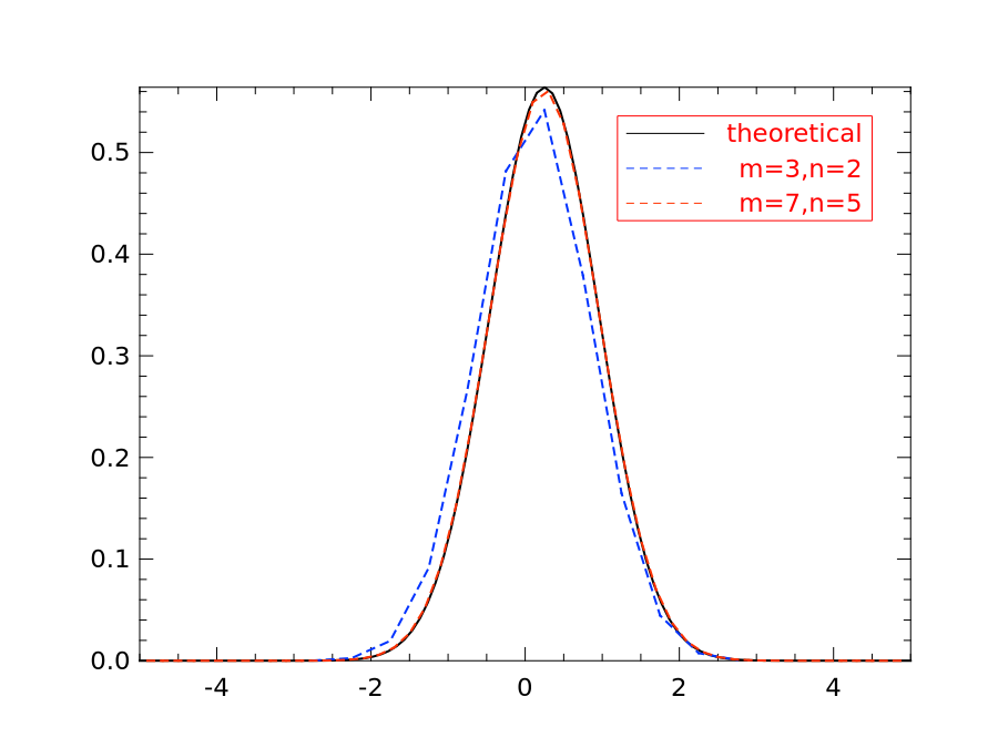
Figure 1. Approximate posteriors

Since all classes induced by $q_{mn}$ have positive $\mu$-mass, approximants can be computed simply as:

$$f^{m,n}([k])([l])={\mu[k]}^{-1}\int_{x\in[k]}\mathcal{N}(x,1)([l])~{}d\mu$$

where $[k]$, $[l]$ range over classes of $q_{mn}$. The corresponding stochastic matrices are shown in Fig. 3 and 3 for $m,n=5,3$ and $6,10$ respectively.

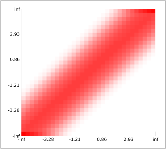
Figure 2. Log-likelihood of $f^{5,3}$

Figure 3. Log-likelihood of $f^{6,10}$

Since these approximants are finite, their Bayesian inverse can be computed directly by Bayes theorem (i.e. taking the adjoint of the stochastic matrices):

(12) $${f^{m,n}}^{\dagger}([l])([k])=\frac{\mu[k]\cdot f^{m,n}([k])([l])}{\nu[l]}$$

with $\nu=f_{*}(\mu)$. Commutation of inversion and approximation guarantees that the $f^{m,n}{}^{\dagger}$ converge to $f^{\dagger}$.

Indeed, Fig. 1 shows the the Lebesgue density of $f^{m,n}{}^{\dagger}(0.5)$ for $m,n=3,2$ (in dashed blue) and $7,5$ (dashed red). The latter approximant is already hardly distinguishable from the exact solution (solid black).

It must be emphasized that this example is meant only as an illustration and does not constitute a universal solution to the irreducibly hard (not even computable in general  (Ackerman et al., 2011)) problem of performing Bayesian inversion. Also, not all quotients are equally convenient: what makes the approach computationally tractable is that the fibres are easily described and the measure conveniently evaluated on such fibres.

7.2. Approximating the Kleene star of ProbNetKAT

ProbNetKAT ((Foster et al., 2016; Smolka et al., 2017)) is a probabilistic network specification language extending Kleene Algebras with Tests ((Kozen, 1997)) with network primitives and a binary probabilistic choice operator $\oplus_{\lambda},\lambda\in\left[0,1\right]$. For the purpose of the example shown here we will not need to introduce the full syntax and semantics of ProbNetKAT, rather we will focus on a single ProbNetKAT program which we will call $\mathtt{cantor}$ and is given by:

(13) $$\mathtt{cantor}:=\tt p;(dup;p)^{*}\quad\text{where}\quad p:=\pi_{0}!\oplus_{\nicefrac{{1}}{{2}}}\pi_{1}!$$

The program acts on sets of finite sequences of 0 and 1, which can be thought of as packet histories. We will write $H$ for the set $\{0,1\}^{*}$ of all packet histories and $H_{n}$ for the set of histories of length as most $n$. A ProbNetKAT program is always interpreted as a kernel $2^{H}\to\mathsf{G}2^{H}$. Programs with both $\tt dup$ and ^∗ revealed to be quite complex from the earliest development of the language. As we will describe, $\mathtt{cantor}$ denotes a continuous distribution and hence having a way to approximate it is crucial for practical uses of the language. The denotation of $\pi_{0}!$ on a single sequence $\{\mathtt{(a_{0},\ldots,a_{n})}\}$ is:

$$\tt\llbracket\pi_{0}!\rrbracket(\{(a_{0},\ldots,a_{n})\})=\delta_{\{(0,a_{1},\ldots,a_{n})\}}$$

in other words $\pi_{0}!$ overwrites the first entry in the sequence with $\tt 0$. Similarly, $\pi_{1}!$ overwrites the first entry with $\tt 1$. This semantics is extended to sets of sequences in the obvious way by taking direct images. The semantics of $\mathtt{p}$ is thus:

$$\llbracket\mathtt{p}\rrbracket(a)=\text{0.5}\delta_{\llbracket\pi_{0}!\rrbracket(a)}+\text{0.5}\delta_{\llbracket\pi_{1}!\rrbracket(a)}$$

The denotation of $\tt dup$ is given on singleton histories by

$$\tt\llbracket dup\rrbracket(\{(a_{0},\ldots,a_{n})\})=\delta_{\{(a_{0},a_{0},\ldots,a_{n})\}}$$

i.e. $\tt dup$ shifts the history to the right and duplicates the first entry. Again, this is extended to sets of histories by taking direct images. The sequential composition operator ; is interpreted by Kleisli composition.

The interpretation of the Kleene star is more involved, and we here describe it categorically. To avoid any confusion we will not use Kleisli arrows in this construction, i.e. all kernels will be explicitly typed as kernels. Note first that the infinite product $(2^{H})^{\omega}$ can be defined as the limit of the ccd given by the maps $q_{n+1,n}:(2^{H})^{n+1}\to(2^{H})^{n}$ dropping the last component. By Bochner’s theorem ((Dahlqvist et al., 2016a)) this also holds of $\mathsf{G}((2^{H})^{\omega})$. Next, consider any program $\tt r$. We turn $2^{H}$ into a cone for the diagram with limit $\mathsf{G}((2^{H})^{\omega})$ via the inductively defined maps:

(14) $$a_{1} =\eta\otimes\llbracket\mathtt{r}\rrbracket\bullet\Delta_{1}:2^{H}\to\mathsf{G}(2^{H}\times 2^{H})$$

(15) $$a_{n} =a_{n-1}\otimes\llbracket\mathtt{r}\rrbracket\bullet\Delta_{n}:(2^{H})^{n}\to\mathsf{G}((2^{H})^{n}\times 2^{H})$$

where $\Delta_{n}:(2^{H})^{n}\to(2^{H})^{n}\times 2^{H}$ is the map copying the last entry. It is easy to check $q_{n+1,n}\bullet a_{n}\bullet a_{n-1}\bullet\ldots\bullet a_{1}=a_{n-1}\bullet\ldots\bullet a_{1}$, and the diagram described by the morphisms $b_{n}:=a_{n}\bullet\ldots\bullet a_{1}:2^{H}\to\mathsf{G}(2^{H})^{n}$ makes $2^{H}$ a cone for $\varprojlim\mathsf{G}(2^{H})^{n}$. There must therefore exist a unique morphism

$$\llbracket\mathtt{r}\rrbracket_{\infty}:2^{H}\to\mathsf{G}\left((2^{H})^{\infty}\right).$$

For each input, this kernel builds a distribution on the sample paths of the discrete-time stochastic processes associated with $\tt r$ and this input. We now define

$$\llbracket\mathtt{r}^{*}\rrbracket:=\mathsf{G}\left(\bigcup\right)\circ\llbracket\tt r\rrbracket_{\infty}$$

where $\bigcup:(2^{H})^{\infty}\to 2^{H}$ is the map taking infinitary unions. Since the definition above makes sense for any kernel $f$ on $2^{H}$, we will overload the Kleene star and put $f^{*}:=\mathsf{G}\bigcup\circ f_{\infty}$. Given the input $\tt(0)$, a sample path of $\mathtt{cantor}$ will draw uniformly a history of size 1, then a history of size 2 whose suffix matches the size 1 history drawn at the previous step, and so on for every integer. The distribution $\llbracket\mathtt{cantor}\rrbracket\mathtt{(0)}$ associates to a measurable collection of sets of histories $A$ the probability that the union of a sample path from $\tt(0)$ belongs to $A$. For example $\llbracket\mathtt{cantor}\rrbracket\mathtt{(0)}\{A\mid(\mathtt{01})\in A\}=\nicefrac{{1}}{{4}}$, since there’s a $\nicefrac{{1}}{{4}}$ chance that a sample path will have drawn $(\mathtt{01})$ amongst the histories of size 2.

We start by turning $2^{H}$ into a $\mathbf{Krn}$-object. Consider the countable directed diagram given by all injections $i_{mn}:H_{m}\to H_{n},n>m$, then $H=\varinjlim H_{n}$, and it follows that $2^{H}=\varprojlim 2^{H_{n}}$ since $2^{-}$ turns colimits into limits. We know from Bochner’s theorem that $\mathsf{G}2^{H}=\varprojlim\mathsf{G}2^{H_{n}}$, and we use this fact to place a canonical measure on $2^{H}$ as follows: since each $2^{H_{n}}$ is finite with cardinality $c_{n}:=2^{\sum_{i}^{n}2^{i}}=2^{2^{n+1}-1}$, and can thus be equipped with the uniform measure $\nicefrac{{1}}{{c_{n}}}$, we can find a limit measure $\mu$ on $2^{H}$ with the pleasing property that for all history truncating maps $p_{n}:2^{H}\to 2^{H_{n}}$, the pushforward $\mu_{n}:=(p_{n})_{*}\mu$ is the uniform measure on $H_{n}$. It is clear that these maps define a discretization scheme on $2^{H}$ which satisfies the condition of Theorem 3. We will now show that if $f^{n}{\longrightarrow}_{\mathrm{s}}f$, then $(f^{n})^{\ast}{\longrightarrow}_{\mathrm{s}}f^{\ast}$. To prove this we need the following lemma which is interesting in its own right.

Lemma 1.

The monoidal structure of $\mathbf{Krn}$ is continuous for the SOT, i.e. $f^{n}{\longrightarrow}_{\mathrm{s}}f$ and $g^{n}{\longrightarrow}_{\mathrm{s}}g$ implies $f^{n}\otimes g^{n}{\longrightarrow}_{\mathrm{s}}f\otimes g$.

Theorem 2.

Under the set-up described above, for any kernel $f:(2^{H},\mu)\rightarrowtriangle(2^{H},\nu)$ we have $(f^{n})^{\ast}{\longrightarrow}_{\mathrm{s}}f^{\ast}$

The advantage of working over finite spaces is that $(f^{n})^{\ast}$ can, in principle at least, be computed for kernels defined in ProbNetKAT. Let us examine this in the case of $\mathtt{cantor}$ and of the discretization scheme $p_{n}:2^{H}\to 2^{H_{n}}$.

In the case $n=3$ the underlying Markov chain has $2^{7}$ states, but has an interesting property which means we need not consider them all: when we compute $\tt\llbracket p\rrbracket;\llbracket(dup;p)\rrbracket_{\infty}^{3}$, the process necessarily lands in an ergodic component of the chain consisting of the singletons of histories of length exactly 3. The reason is that once the process reaches histories of length 3 it starts randomly re-writing the histories, and with probability 1 any two histories will eventually get re-written to the same thing. Once a set of histories has decreased in cardinality by one, it can never go back, thus eventually any set of histories gets re-written to a single length 3 history, and then loops among length 3 singletons indefinitely. The situation is represented from the initial state $\tt(0)$ in Figure 4 where, for clarity’s sake, the ergodic component is symbolized by common double-sided arrows to a new state.

Figure 4. $\tt\llbracket p\rrbracket;\llbracket(dup;p)\rrbracket_{\infty}^{3})$ starting at $\tt(0)$

By post-composing with $\mathsf{G}\bigcup$ we have

$$\llbracket\mathtt{p}\rrbracket;(\llbracket\mathtt{(dup;p)}\rrbracket^{3})^{\ast}(a)(A)=0$$

if $A$ does not contain all histories of length 3. We have meaningful answers to questions about histories up to length 2:

$$\llbracket\mathtt{p}\rrbracket;(\llbracket\mathtt{(dup;p)}\rrbracket^{3})^{\ast}(\mathtt{(0)})(\{A\mid\mathtt{(1)}\in A\})=0.5$$

$$\llbracket\mathtt{p}\rrbracket;(\llbracket\mathtt{(dup;p)}\rrbracket^{3})^{\ast}(\mathtt{(0)})(\{A\mid\mathtt{(10)}\in A\})=0.25$$

In other words, at $n=3$ we have the first two steps in the construction of the Cantor distribution towards which $\mathtt{cantor}$ converges.

8. Conclusion

We have presented a framework for the exact and approximate semantics of first-order probabilistic programming. The semantics can be read off either in terms of kernels between measured spaces, or in terms of operators between $\mathrm{L}_{p}$ spaces. Either forms come with related involutive structures: Bayesian inversion for (measured) kernels between Standard Borel spaces, and Köthe duality for positive linear and $\sigma$-continuous operators between Banach lattices. Functorial relations between both forms can themselves be related by way of natural isomorphisms. Our main result is the convergence of general systems of finite approximants in terms of the strong operator topology (the SOT theorem). Thus, in principle, one can compute arbitrarily good approximations of the semantics of a probabilistic program of interest for any given (measurable) query. Future work may allow one to derive stronger notions of convergences given additional Lipschitz control on kernels, or to develop approximation schemes that are adapted to the measured kernel of interest. More ambitiously perhaps, one could investigate whether MCMC sampling schemes commonly used to perform approximate Bayesian inference in the context of probabilistic programming could be seen as randomized approximations of the type considered in this paper.

Appendix A Appendix

Proof of Theorem 1.
This is a consequence of the Isomorphism Theorem (Theorem 15.6 of (Kechris, 1995)): two SB spaces are isomorphic iff they have the same cardinality. Uncountable SB spaces are thus all isomorphic to the Cantor space $2^{\mathbb{N}}$ which is the limit of the countable co-directed diagram $(2^{n})_{n\in\mathbb{N}}$ with the connecting morphisms $p_{n+1,n}:2^{n+1}\to 2^{n}$ truncating binary words of length $n+1$ at length $n$. Similarly all SB-spaces of cardinality $\aleph_{0}$ are isomorphic to the one-point compactification of $\mathbb{N}$, which is the limit of the countable co-directed diagram $(n)_{n\in\mathbb{N}}$ with the connecting morphisms $p_{n+1,n}:n+1\to n,i\mapsto\min(i,n)$. The case of finite SB spaces is trivial.

$\blacksquare$

Proof of Lemma 3.
By Dinkyn’s $\pi$-$\lambda$ theorem, two finite measures are equal if and only if they agree on a $\pi$-system generating the $\sigma$-algebra. Any standard Borel space admits such a countable $\pi$-system (any countable basis for a Polish topology generating the $\sigma$-algebra). Let $\{B_{n}\}_{n\in\mathbb{N}}$ be such a $\pi$-system. Then, for all $x\in X$, $g(x)\neq g^{\prime}(x)\Leftrightarrow\exists n.g(x)(B_{n})\neq g^{\prime}(x)(B_{n})$. Hence,

$$\begin{array}[]{lll}N(g,g^{\prime})&=&\cup_{n}\{x\in X\mid g(x)(B_{n})\neq g^{\prime}(x)(B_{n})\}\\ &=&\cup_{n}\{x\in X\mid ev_{B_{n}}(g(x))\neq ev_{B_{n}}(g^{\prime}(x))\}\\ &=&\cup_{n}(ev_{B_{n}}\circ g-ev_{B_{n}}\circ g^{\prime})^{-1}(\mathbb{R}\setminus\{0\})\\ \end{array}$$

By definition of the measurable structure of $\mathsf{G}(Y)$, $ev_{B_{n}}\circ g-ev_{B_{n}}\circ g^{\prime}$ is measurable, hence $N(g,g^{\prime})$ is also measurable.

$\blacksquare$

Proof of Proposition 4.
We first show that if $g\sim g^{\prime}$, then $h\bullet g\sim h\bullet g^{\prime}$. Clearly, for any space $V$ and any deterministic function $u:Y\to V$, $N(u\circ g,u\circ g^{\prime})\subseteq N(g,g^{\prime})$. By definition of the Kleisli category, $h\bullet g=m_{Z}\circ\mathsf{G}(h)\circ g$ and similarly for $h\bullet g^{\prime}$. Taking $u=m_{Z}\circ\mathsf{G}(h)$, we obtain that $\mu(N(h\bullet g,h\bullet g^{\prime}))\leq\mu(N(g,g^{\prime}))$.

It is now enough to show that $\lambda(N(g\bullet f,g^{\prime}\bullet f))=0$. Let us reason contrapositively. We have:

$$\begin{array}[]{llll}&\lambda(N(g\bullet f,g^{\prime}\bullet f))&>0\\ \Leftrightarrow&\int_{w\in W}1_{N(g\bullet f,g^{\prime}\bullet f)}(w)\>d\lambda&>0\\ \to&\int_{w\in W}\sum_{n\in\mathbb{N}}1_{(g\bullet f)(w)(B_{n})\neq(g^{\prime}\bullet f)(w)(B_{n})}\>d\lambda&>0\\ \stackrel{{\scriptstyle\exists n}}{{\to}}&\int_{w\in W}1_{(g\bullet f)(w)(B_{n})\neq(g^{\prime}\bullet f)(w)(B_{n})}\>d\lambda&>0\\ \to&\int_{w\in W}\left|(g\bullet f)(w)(B_{n})-(g^{\prime}\bullet f)(w)(B_{n})\right|\>d\lambda&>0\\ \Leftrightarrow&\int_{w\in W}\int_{x\in X}\left|g(x)(B_{n})-g^{\prime}(x)(B_{n})\right|~{}df(w)\>d\lambda&>0\\ \Leftrightarrow&\int_{x\in X}\left|g(x)(B_{n})-g^{\prime}(x)(B_{n})\right|\>d\mu&>0\\ \stackrel{{\scriptstyle\exists X^{+}\subseteq X}}{{\to}}&\int_{x\in X^{+}}g(x)(B_{n})-g^{\prime}(x)(B_{n})\>d\mu&>0\\ \to&\int_{x\in X^{+}}1_{g(-)(B_{n})>g^{\prime}(-)(B_{n})}(x)\>d\mu&>0\\ \to&\int_{x\in X^{+}}1_{N(g,g^{\prime})}(x)\>d\mu&>0\\ \end{array}$$

The last line implies $\mu(N(g,g^{\prime}))>0$, a contradiction.

$\blacksquare$

Proof of Theorem 6.
If $\phi$ is $\nu$-integrable, there exists a monotone sequence $\{\phi_{n}\}$ of simple functions such that $\phi_{n}\uparrow\phi$ and $\int_{Y}\phi_{n}d\nu\to\int_{Y}\phi d\nu<\infty$. By definition each $\phi_{n}=\sum_{i=0}^{k}\alpha_{i}1_{B_{i}}$, and by unravelling the definition we have

$$\int_{Y}1_{B_{i}}d\nu =\nu(B_{i})$$

$$=\int_{X}f(x)(B_{i})d\mu$$

$$=\int_{X}\int_{Y}1_{B_{i}}df(x)d\mu$$

$$=\int_{X}(1_{B_{i}}\bullet f)d\mu$$

From which it follows that

$$\int_{Y}\phi_{n}d\nu=\int_{X}\int_{Y}\sum_{i=0}^{k}\alpha_{i}1_{B_{i}}df(x)d\mu=\int_{X}(\phi_{n}\bullet f)d\mu$$

and the result follows from the Monotone Convergence Theorem (MCT).

$\blacksquare$

Proof of Theorem 9.
It follows by definition of $f^{\dagger}$ and from the disintegration theorem that

(16) $$\int_{y\in Y}f^{\dagger}(y)(A)\cdot 1_{B}(y)~{}d\nu=\gamma_{f}(A\times B),$$

from which Eq. 4 follows easily. It remains to prove that this uniquely characterizes $f^{\dagger}$. Let us reason contrapositively. Assume there exists $g:(Y,\nu)\rightarrowtriangle(X,\mu)$ verifying for all $A,B$ measurable $\int_{y\in Y}g(y)(A)\cdot 1_{B}(y)=\gamma_{f}(A\times B)$ as in Eq. 16 and such that $\nu(N(f^{\dagger},g))>0$ (assuming we take some representative of $f^{\dagger}$). Let $\{A_{n}\}_{n\in\mathbb{N}}$ be a countable $\pi$-system generating the $\sigma$-algebra of $X$. It is enough to test equality of measures on $X$ on this $\pi$-system. Therefore, $N(f^{\dagger},g)=\cup_{n}\{y\mid f^{\dagger}(y)(A_{n})\neq g(y)(A_{n})\}$. Since $\nu(N(f^{\dagger},g))>0$, there must exist a $k\in\mathbb{N}$ such that $\nu(\{y\mid f^{\dagger}(y)(A_{k})\neq g(y)(A_{k})\})>0$. Therefore, $N_{k}^{+}=\{y\mid f^{\dagger}(y)(A_{k})>g(y)(A_{k})\}$ must also have positive measure for $\nu$. But then, $\int_{y\in Y}g(y)(A_{k})\cdot 1_{N_{k}^{+}}(y)\neq\gamma_{f}(A_{k}\times N_{k}^{+})$, a contradiction.

$\blacksquare$

Proof of Theorem 10.
Let us first show that $(-)^{\dagger}$ is a functor $\mathbf{Krn}\to\mathbf{Krn}^{\mathrm{op}}$, i.e. that $\mathrm{id}_{(X,\mu)}^{\dagger}=\mathrm{id}_{(X,\mu)}$ and that for any $f:(X,\mu)\rightarrowtriangle(Y,\nu)$ and $g:(Y,\nu)\rightarrowtriangle(Z,\rho)$ we have $(g\bullet f)^{\dagger}=f^{\dagger}\circ g^{\dagger}$.

Let $(X,\mu)$ be an object of $\mathbf{Krn}$ and $\mathrm{id}_{X,\mu}$ the corresponding identity. By Th. 9, it is enough to prove, for all $A,A^{\prime}$ measurable subsets of $X$, that

$$\int_{x\in X}1_{A}(x)\cdot id_{X,\mu}(x)(A^{\prime})~{}d\mu=\int_{x\in X}id_{X,\mu}(x)(A)\cdot 1_{A^{\prime}}(x)~{}d\mu.$$

We have:

$$\int_{x\in X}1_{A}(x)\cdot id_{X,\mu}(x)(A^{\prime})~{}d\mu=\int_{x\in X}1_{A}(x)\cdot 1_{A^{\prime}}~{}d\mu=\mu(A\cap A^{\prime})$$

The same calculation on the right hand side of the first equation yields trivially the same result. Hence the equality is verified.

Now, on to compatibility w.r.t. composition. In sight of Th. 9, it is enough to show that for all $A\subseteq X$, $C\subseteq Z$,

$$\int_{x\in X}(g\bullet f)(x)(C)\cdot 1_{A}(x)~{}d\mu=\int_{z\in Z}1_{C}(z)\cdot(f^{\dagger}\bullet g^{\dagger})(z)(A)~{}d\rho$$

In the following, for $X$ a measurable space, we denote by $SF(X)$ the set of simple functions over $X$ (finite linear combinations of indicator functions of measurable sets). We will use repeatedly the monotone convergence theorem (MCT). The left hand side of the above equation can be re-written as:

$$\begin{array}[]{ll}&\int_{x\in X}\left(\int_{y\in Y}g(y)(C)~{}df(x)\right)\cdot 1_{A}(x)~{}d\mu\\ \stackrel{{\scriptstyle(1)}}{{=}}&\int_{x\in X}\left(\int_{y\in Y}\lim_{n\to\infty}g_{n}(y)~{}df(x)\right)\cdot 1_{A}(x)~{}d\mu\\ \stackrel{{\scriptstyle(2)}}{{=}}&\int_{x\in X}\lim_{n\to\infty}\left(\int_{y\in Y}g_{n}(y)~{}df(x)\right)\cdot 1_{A}(x)~{}d\mu\\ \end{array}$$

where $(1)$ is because $g_{n}\uparrow g(-)(C),g_{n}\in SF(Y)$ and $(2)$ by monotone convergence. Note that the $n$-indexed family $x\mapsto\int_{y\in Y}g_{n}(y)~{}df(x)$ is pointwise increasing. Therefore,

$$\begin{array}[]{ll}{}^{(\ast)}&\lim_{n\to\infty}\int_{x\in X}\left(\int_{y\in Y}g_{n}(y)~{}df(x)\right)\cdot 1_{A}(x)~{}d\mu\\ \stackrel{{\scriptstyle(1)}}{{=}}&\lim_{n\to\infty}\int_{x\in X}\left(\sum_{i=1}^{k_{n}}\alpha_{i}^{n}f(x)(C_{i}^{n})\right)\cdot 1_{A}(x)~{}d\mu\\ =&\lim_{n\to\infty}\sum_{i=1}^{k_{n}}\alpha_{i}^{n}\int_{x\in X}f(x)(C_{i}^{n})\cdot 1_{A}(x)~{}d\mu\\ \stackrel{{\scriptstyle(2)}}{{=}}&\lim_{n\to\infty}\sum_{i=1}^{k_{n}}\alpha_{i}^{n}\int_{y\in Y}1_{C_{i}^{n}}(y)\cdot f^{\dagger}(y)(A)~{}d\nu\\ \stackrel{{\scriptstyle(\ast)}}{{=}}&\int_{y\in Y}g(y)(C)\cdot f^{\dagger}(y)(A)~{}d\nu\\ \stackrel{{\scriptstyle(3)}}{{=}}&\int_{y\in Y}g(y)(C)\cdot\lim_{n}f_{n}(y)~{}d\nu\\ \stackrel{{\scriptstyle(\ast)}}{{=}}&\lim_{n}\sum_{i=1}^{k_{n}}\beta_{i}^{n}\int_{y\in Y}g(y)(C)\cdot 1_{D_{i}^{n}}(y)~{}d\nu\\ \stackrel{{\scriptstyle(2)}}{{=}}&\lim_{n}\sum_{i=1}^{k_{n}}\beta_{i}^{n}\int_{z\in Z}1_{C}(z)\cdot g^{\dagger}(z)(D_{i}^{n})~{}d\rho\\ =&\lim_{n}\int_{z\in Z}1_{C}(z)\cdot\int_{y\in Y}\sum_{i=1}^{k_{n}}\beta_{i}^{n}1_{D_{i}^{n}}(y)~{}dg^{\dagger}(z)~{}d\rho\\ \stackrel{{\scriptstyle(\ast)}}{{=}}&\int_{z\in Z}1_{C}(z)\cdot\int_{y\in Y}f^{\dagger}(y)(C)~{}dg^{\dagger}(z)~{}d\rho\\ =&\int_{z\in Z}1_{C}(z)\cdot(f^{\dagger}\bullet g^{\dagger})(z)(A)~{}d\rho\end{array}$$

where $(\ast)$ is by monotone convergence, $(1)$ is because $g_{n}\in SF(Y)$, $(2)$ is by Th. 9 and $(3)$ is because $f_{n}\uparrow f^{\dagger}(-)(A),f_{n}\in SF(Y)$. We have proved the sought identity.

Finally let us show that $(-)^{\dagger}$ is involutive, i.e. that for any $f:(X,\mu)\rightarrowtriangle(Y,\nu)$, $(f^{\dagger})^{\dagger}=f$. This follows easily by two applications of Th. 9): we have

$$\begin{array}[]{lll}\int_{x\in X}1_{A}(x)\cdot(f^{\dagger})^{\dagger}(x)(B)~{}d\mu&=&\int_{y\in Y}f^{\dagger}(y)(A)\cdot 1_{B}(y)~{}d\nu\\ &=&\int_{x\in X}1_{A}(x)\cdot f(x)(B)~{}d\mu;\end{array}$$

and since adjoints are unique, $f=(f^{\dagger})^{\dagger}$.

The fact that $(f\otimes g)^{\dagger}=f^{\dagger}\otimes g^{\dagger}$ follows immediately from the definitions and the property of disintegrations given by Th. 9. The fact that the associator, unitors and braiding transformations are unitary follows immediately from the fact that they are deterministic isomorphisms and Th. 7.

$\blacksquare$

Proof of Proposition 2.
Let $B\subseteq Y$ be a measurable set. By definition, we have $(f\bullet\rho)(B)=\int_{X}ev_{B}\circ f~{}d\rho$ where we recall that $ev_{B}:\mathsf{G}(X)\to\mathbb{R}_{+}$ is the evaluation morphism. Let $\{f^{B}_{n}\}_{n\in\mathbb{N}}$ be an increasing chain of simple functions converging pointwise to $ev_{B}\circ f$ such that for each $n$, $f^{B}_{n}=\sum_{i=1}^{k_{n}}\alpha_{i}^{n}1_{A_{i}^{n}}$ with $\alpha_{i}^{n}\geq 0$. By the MCT,

$$(f\bullet\rho)(B)=\lim_{n}\int_{X}f^{B}_{n}~{}d\rho=\lim_{n}\sum_{i=1}^{k_{n}}\alpha_{i}^{n}\rho(A_{i}^{n}).$$

Similarly,

$$\nu(B)=(f\bullet\mu)(B)=\lim_{n}\int_{X}f^{B}_{n}~{}d\mu=\lim_{n}\sum_{i=1}^{k_{n}}\alpha_{i}^{n}\mu(A_{i}^{n}).$$

Notice that since the integral is linear and the sequence $\{f_{n}^{B}\}_{n}$ is increasing, the sequences $\{\int_{X}f^{B}_{n}~{}d\rho\}_{n}$ and $\{\int_{X}f^{B}_{n}~{}d\mu\}_{n}$ are also increasing. Assume $\nu(B)=0$. Then for all $n$, $\int_{X}f^{B}_{n}~{}d\mu=0$. We deduce that for all $n$, for all $1\leq i\leq k_{n}$, either $\alpha_{i}^{n}=0$ or $\mu(A_{i}^{n})=0$. Using that $\rho\ll\mu$, we deduce that for all $1\leq i\leq k_{n}$, either $\alpha_{i}^{n}=0$ or $\rho(A_{i}^{n})=0$, from which we conclude that for all $n$, $\int_{X}f^{B}_{n}~{}d\rho=0$ and finally, $(f\bullet\rho)(B)=0$. Hence, $f\bullet\rho\ll\nu$.

$\blacksquare$

Proof of Theorem 3.
We start by proving the following Lemma

Lemma 1.

For any $f:(X,\mu)\rightarrowtriangle(Y,\nu)$, $\phi\in\mathrm{L}_{1}(Y,\nu)$, and $B_{X}\subseteq X$ measurable

$$\int_{B_{X}}\left(\int_{Y}\phi df(x)\right)~{}d\mu=\int_{Y}\phi(y)f^{\dagger}(y)(B_{X})~{}d\nu$$

Proof.

We start by showing the equation on characteristic functions. If $B_{Y}$ is measurable in $Y$, we have

$$\int_{B_{X}}\left(\int_{Y}1_{B_{Y}}df(x)\right)~{}d\mu =\int_{B_{X}}f(x)(B_{Y})~{}d\mu$$

$$=\int_{Y}1_{B_{Y}}(y)f^{\dagger}(y)(B_{X})~{}d\nu$$ Eq. (4)

Since $\phi$ is measurable and integrable, there exists a sequence $\phi_{n}\uparrow\phi$ of simple functions such that $\lim_{n}\int_{Y}\phi_{n}~{}d\nu<\infty$, and the results follows by the linearity of integration and the MCT. ∎

We can now prove the naturality of $\mathsf{rn}$. Let $f:(X,\mu)\rightarrowtriangle(Y,\nu)$ be a morphism in $\mathbf{Krn}$; we have on the one hand

$$\mathsf{rn}_{(Y,\mu)}\circ\mathcal{M}^{\ll\cdot}(f)(\rho)(y) =\mathsf{rn}_{(Y,\nu)}(\int_{X}f(x)(-)~{}d\rho)(y)$$

$$=\frac{d\int_{X}f(x)(-)d\rho}{d\nu}(y) (*)$$

and on the other

$$\mathsf{T}_{1}(f^{\dagger})\circ\mathsf{rn}_{(X,\mu)}(\rho)(y) =\mathsf{T}_{p}(f^{\dagger})\left(\frac{d\rho}{d\mu}\right)(y)$$

$$=\int_{X}\frac{d\rho}{d\mu}~{}df^{\dagger}(y) (**)$$

To show the equality of these two maps in $\mathrm{L}_{1}(Y,\nu)$ it is enough to show that they are equal $\nu$-a.e. To see this, we show that $(**)$ satisfies the condition to be the Radon-Nikodym derivative $(*)$. Let $B_{Y}$ be a measurable subset of $Y$. We have from the well-known property of Radon-Nikodym derivatives:

$$\int_{B_{Y}}\frac{d\int_{X}f(x)(-)~{}d\rho}{d\nu}d\nu=\int_{x\in X}f(x)(B_{Y})~{}d\rho$$

Moreover, we have

$$\int_{B_{Y}}\int_{X}\frac{d\rho}{d\mu}~{}df^{\dagger}(y)~{}d\nu \stackrel{{\scriptstyle(1)}}{{=}}\int_{x\in X}\frac{d\rho}{d\mu}(x)f(x)(B_{Y})~{}d\mu$$

$$\stackrel{{\scriptstyle(2)}}{{=}}\int_{x\in X}f(x)(B)~{}d\rho$$

where $(1)$ is by Lemma 1 and $(2)$ is a well-known property of Radon-Nikodym derivatives.

$\blacksquare$

Proof of Theorem 4.
We start with the following elementary lemma.

Lemma 2.

If $\psi,\phi\in\mathrm{L}_{1}(X,\mu)$ then

$$\int_{X}\psi\phi~{}d\mu=\int_{X}\psi~{}d(\mathsf{mr}_{(M,\mu)}\phi)$$

Proof.

The proof of naturality now follows easily: it is enough to show the equality in the case where $\psi=1_{B_{X}}$ for a measurable subset $B_{X}$ of $X$, and the result then extends to all measurable functions by linearity of integrals and the MCT. We have

$$\int_{X}1_{B_{X}}\phi~{}d\mu=\int_{B_{X}}\phi d\mu :=\mathsf{mr}_{(M,\mu)}(\phi)(B_{X})$$

$$=\int_{X}1_{B_{X}}~{}d(\mathsf{mr}_{(M,\mu)}(\phi))$$

∎

To show naturality we now let $f:(X,\mu)\rightarrowtriangle(Y,\nu)$ be a $\mathbf{Krn}$-morphism, $\phi\in\mathrm{L}_{1}(X,\mu)$ and $B_{Y}$ measurable in $Y$

$$\mathsf{mr}_{(Y,\nu)}\mathsf{T}_{1}(f^{\dagger})(\phi)(B_{X})$$

$$=\mathsf{mr}_{(Y,\nu)}(\phi\bullet f^{\dagger})(B_{Y})$$

$$=\int_{B_{Y}}\phi\bullet f^{\dagger}~{}d\nu$$

$$=\int_{B_{Y}}\int_{X}\phi df^{\dagger}(y)~{}d\nu$$

$$=\int_{X}f(x)(B_{Y})\phi(x)~{}d\mu$$ Lemma 1

$$=\int_{X}f(x)(B_{Y})~{}d(\d{(}\mathsf{mr}_{(X,\mu)}(\phi))$$ Lemma 2

$$=\mathcal{M}^{\ll\cdot}f\circ\mathsf{mr}_{(X,\mu)}(\phi)(B_{Y})$$

$\blacksquare$

Proof of Theorem 5.
Again, we start with a simple but helpful Lemma.

Lemma 3.

Let $F\in(\mathsf{S}_{\infty}(X,\mu)^{\sigma}$ and $\phi\in\mathsf{S}_{\infty}(X,\mu)$, then

$$F(\phi)=\int_{X}\phi~{}d(\mathsf{rr}_{(X,\mu)}(F))$$

Proof.

Starting with characteristic functions, let $\phi=1_{B}$ for some measurable subset $B$ of $X$. We then have

$$F(1_{B}):=\mathsf{rr}_{(X,\mu)}(F)(B)=\int_{X}1_{B}~{}d(\mathsf{rr}_{(X,\mu)}(F))$$

We can then extend the result to simple functions by linearity and then to all functions in $\mathrm{L}_{\infty}(X,\mu)$ by the MCT. ∎

To show naturality we now let $f:(X,\mu)\rightarrowtriangle(Y,\nu)$ be a $\mathbf{Krn}$-morphism, $F\in(\mathsf{S}_{\infty}(X,\mu))^{\sigma}$ and $B_{Y}$ measurable in $Y$. We have

$$\mathcal{M}^{\ll\cdot}f\circ\mathsf{rr}_{(X,\mu)}(F)(B_{Y}) =\int_{X}f(x)(B_{Y})~{}d(\mathsf{rr}_{(X,\mu)}(F))$$

$$=F(f(\cdot)(B_{Y}))\qquad\text{Lemma \ref{lem:mrHelp}}$$

$$=F(\int_{X}1_{B_{Y}}df(\cdot))$$

$$=F(1_{B_{Y}}\bullet f)$$

$$=\mathsf{rr}_{(Y,\nu)}(F(-\bullet f))(B_{Y})$$

$$=\mathsf{rr}_{(Y,\nu)}\circ(\mathsf{T}_{1}f)^{\sigma}(F)(B_{Y})$$

$\blacksquare$

Proof of Theorem 6.
We start by showing that $\mathsf{fr}$ is well defined. The linearity of $\mathsf{fr}_{(X,\mu)}$ is easily checked on simple functions and extended by the CMT. Positivity is also immediate. For the $\sigma$-order continuity, let $\mu_{m}\uparrow\mu$, $\phi\in\mathrm{L}_{\infty}(X,\mu)$, and $\phi_{n}\uparrow\phi$ be a monotone approximation of $\phi$ by simple functions. We need to show that

$$\lim_{m\to\infty}\int_{X}\phi~{}d\mu_{m}=\int_{X}\phi~{}d\mu$$

For note first that the doubly indexed series $\int_{X}\phi_{n}d\mu_{m}$ is monotonically increasing in $m$, since the $\mu_{m}$ are monotonically increasing. Note also that the differences

$$d_{mn}:=\int_{X}\phi_{n}~{}d\mu_{m+1}-\int_{X}\phi_{n}~{}d\mu_{m}$$

are monotonically increasing in $n$. Indeed we have

$$\left(\int_{X}\phi_{n+1}~{}d\mu_{m+1}-\int_{X}\phi_{n+1}~{}d\mu_{m}\right)-\left(\int_{X}\phi_{n}d\mu_{m+1}-\int_{X}\phi_{n}~{}d\mu_{m}\right)$$

$$=\int_{X}(\phi_{n+1}-\phi_{n})~{}d\mu_{m+1}-\int_{X}(\phi_{n+1}-\phi_{n})~{}d\mu_{m}>0$$

since the sequences $\phi_{n}$ and $\mu_{m}$ are monotonically increasing. Since $d_{mn}$ is monotonically increasing in $n$ we can apply the CMT to $d_{mn}$ seen as a function of $m$ w.r.t. the counting measure, i.e.

$$\lim_{n\to\infty}\sum_{m}^{\infty}~{}d_{mn}=\sum_{m}^{\infty}\lim_{n\to\infty}~{}d_{mn}$$

which is to say, by taking partial sums

$$\lim_{n\to\infty}\lim_{m\to\infty}\sum_{k=1}^{m}d_{kn} =\lim_{n\to\infty}\lim_{m\to\infty}\int_{X}\phi_{n}~{}d\mu_{m}$$

$$=\lim_{m\to\infty}\sum_{k=1}^{m}\lim_{n\to\infty}d_{kn}$$

$$=\lim_{m\to\infty}\lim_{n\to\infty}\int_{X}\phi_{n}~{}d\mu_{m}$$

which concludes the proof that $\mathsf{fr}$ is well-defined.

We now prove naturality. Let $f:(X,\mu)\rightarrowtriangle(Y,\nu)$ be a $\mathbf{Krn}$-morphism, $\rho\in\mathcal{M}^{\ll\mu}(X)$ and $\phi\in\mathsf{S}_{\infty}(Y,\nu)$ we then have

$$\mathsf{fr}_{(Y,\nu)}\circ\mathcal{M}^{\ll\cdot}f(\rho)(\phi) =\int_{Y}\phi~{}d(\mathcal{M}^{\ll\cdot}f(\rho)(\phi))$$

$$=\int_{Y}(\phi\bullet f)~{}d\rho\qquad\text{Theorem }\ref{thm:chgVarKrn}$$

$$=\mathsf{S}_{\infty}(f)\left(\int_{Y}(-)~{}d\rho\right)(\phi)$$

$$=\mathsf{S}_{\infty}(f)\circ\mathsf{fr}_{(X,\mu)}(\rho)(\phi)$$

$\blacksquare$

Proof of Theorem 7.
The fact that $\mathsf{rn}_{(X,\mu)}$ and $\mathsf{mr}_{(X,\mu)}$ are inverse of each other is just a restatement of the two well-known equalities for Radon-Nikodym derivatives:

$$\frac{d\int_{-}\phi~{}d\mu}{d\mu}=\phi\hskip 4.30554pt\text{ and }\hskip 4.30554pt\int_{B_{X}}\frac{d\rho}{d\mu}~{}d\mu=\rho(B_{X})$$

$\blacksquare$

Proof of Theorem 8.
Let $(X,\mu)$ be a $\mathbf{Krn}$-object, let $F\in(\mathrm{L}_{\infty}(X,\mu))^{\sigma}$ and let $\phi\in\mathrm{L}_{\infty}(X,\mu)$. We have

$$\mathsf{fr}_{(X,\mu)}\circ\mathsf{rr}_{(X,\mu)}(F)(\phi)=\int_{X}\phi~{}d(\mathsf{rr}_{(X,\mu)}(F))=F(\phi)$$

where the last equality follows from Lemma 3. Similarly, we have

$$\mathsf{rr}_{(X,\mu)}\circ\mathsf{fr}_{(X,\mu)}(\rho)(B_{X})=\mathsf{fr}_{(X,\mu)}(\rho)(1_{B_{X})}=\int_{X}1_{B_{X}}d\rho=\rho(B_{X})$$

$\blacksquare$

Proof of Theorem 10.
The case $p=1$ has been treated already, for the case of $1<p<\infty$, see for example the proof of Theorem 4.4.1 of (Bogachev, 2006). Finally for the case of $p=\infty$, see Proposition 3.3 of (Chaput et al., 2014).

$\blacksquare$

Proof of Proposition 2.
Note in (11) that we disintegrate $p$ with respect to two different measures. For notational clarity let us define the endo-kernels

$$a :=p^{\dagger}_{\mu}\bullet p$$

$$b :=p^{\dagger}_{\nu}\bullet p$$

The kernel $a$ associates to each $x\in X$ in a fibre $p^{-1}(\{i\})$ the measure $\pi_{\mu}^{\dagger}(i)$ supported by this fibre. In particular it is constant on each fibre, and similarly for $b$. We can now compute:

$$f^{p}(x)(A)$$

$$:=b\bullet f\bullet a(x)(A)$$

$$=\int_{y\in X}b(y)(A)~{}d(f\bullet a)(x)$$

$$\stackrel{{\scriptstyle(1)}}{{=}}\sum_{i\in X^{\prime}}\int_{y\in p^{-1}(i)}b(y)(A)~{}d(f\bullet a)(x)$$

$$\stackrel{{\scriptstyle(2)}}{{=}}\sum_{i\in X^{\prime}}p_{\nu}^{\dagger}(i)(A\cap p^{-1}(i))f\bullet a(x)(p^{-1}(i))$$

$$=\sum_{i\in X^{\prime}}p_{\nu}^{\dagger}(i)(A\cap p^{-1}(i))\int_{y\in X}f(y)(p^{-1}(i))~{}da(x)$$

$$\stackrel{{\scriptstyle(3)}}{{=}}\sum_{i\in X^{\prime}}p_{\nu}^{\dagger}(i)(A\cap p^{-1}(i))\int_{y\in p^{-1}(p(x))}f(y)(p^{-1}(i))~{}dp_{\mu}^{\dagger}(p(x))$$

where $(1)$ follows by decomposing $X$ in fibres, $(2)$ is because $b(y)(A)$ is constant on fibres, and $(3)$ uses the fact that $a(x):=p_{\mu}^{\dagger}(p(x))$ is supported on the fibre of $p(x)$. We can considerably simplify the expression above. Note first that by definition of the disintegration

(17) $$\nu(A\cap p^{-1}(i))=p^{\dagger}_{\nu}(i)(A\cap p^{-1}(i))\nu(p^{-1}(i))$$

Similarly, by definition of the disintegration, for $i,j\in X^{\prime}$

$$\int_{p^{-1}(j)}f(x)(p^{-1}(i))~{}d\mu$$

$$=\int_{X}1_{p^{-1}(j)}(x)f(x)(p^{-1}(i))~{}d\mu$$

$$=\sum_{k\in X^{\prime}}\mu(p^{-1}(k))\int_{p^{-1}(k)}1_{p^{-1}(j)}(x)f(x)(p^{-1}(i))~{}dp^{\dagger}_{\mu}(k)$$

(18) $$=\mu(p^{-1}(j))\int_{p^{-1}(j)}f(x)(p^{-1}(i))~{}dp^{\dagger}_{\mu}(j)$$

where the last step uses the fact that $p^{\dagger}_{\mu}(k)$ is supported by the fibre over $k$. By multiplying the LHS of (17), (18) we get

$$\nu(A\cap p^{-1}(i))\int_{p^{-1}(j)}f(x)(p^{-1}(i))d\mu$$

$$=\int_{X}f(x)(A\cap p^{-1}(i))d\mu\int_{p^{-1}(j)}f(x)(p^{-1}(i))~{}d\mu$$

$$=\int_{p^{-1}(j)}f(x)(A\cap p^{-1}(i))~{}d\mu\int_{X}f(x)(p^{-1}(i))~{}d\mu$$

$$=\mu(p^{-1}(j))\int_{p^{-1}(j)}f(x)(A\cap p^{-1}(i))~{}dp^{\dagger}_{\mu}(j)\int_{X}f(x)(p^{-1}(i))~{}d\mu$$

(19) $$=\mu(p^{-1}(j))\nu(p^{-1}(A))\int_{p^{-1}(j)}f(x)(A\cap p^{-1}(i))~{}dp^{\dagger}_{\mu}(j)$$

It now follows from (17), (18), and (19) that

$$\mu(p^{-1}(j))\nu(p^{-1}(A))\int_{p^{-1}(j)}f(x)(A\cap p^{-1}(i))~{}dp^{\dagger}_{\mu}(j)$$

$$=p^{\dagger}_{\nu}(i)(A\cap p^{-1}(i))\nu(p^{-1}(i))\mu(p^{-1}(j))\int_{p^{-1}(j)}f(x)(p^{-1}(i))~{}dp^{\dagger}_{\mu}(j)$$

Which simplifies to

$$\int_{p^{-1}(j)}f(x)(A\cap p^{-1}(i))~{}dp^{\dagger}_{\mu}(j)$$

(20) $$=p^{\dagger}_{\nu}(i)(A\cap p^{-1}(i))\int_{p^{-1}(j)}f(x)(p^{-1}(i))~{}dp^{\dagger}_{\mu}(j)$$

We can now use (20) to get

$$b\bullet f\bullet a(x)(A)$$

$$=\sum_{i\in X^{\prime}}\int_{p^{-1}(\pi(x))}f(x)(A\cap p^{-1}(i))~{}dp^{\dagger}_{\mu}(p(x))$$

(21) $$=\int_{p^{-1}(p(x))}f(x)(A)~{}dp^{\dagger}_{\mu}(p(x))=f\bullet a(x)(A)$$

$\blacksquare$

Proof of Lemma 2.
The map $f(-)(A):X\to\mathbb{R}$ defines a random variable, and the discretization scheme defines a filtration $\sigma(p_{n})\subseteq\sigma(p_{n+1})$ whose union is $\mathcal{B}_{X}$. Following Lemma 8 and Proposition 2 we have

$$f^{n}(x)(A):=f(x)(A)\bullet p_{n}^{\dagger}\bullet p_{n}=\mathbb{E}\left[f(x)(A)\mid\sigma(p_{n})\right]$$

We thus have a sequence $f^{n}(-)(A)$ of random variables $X\to\mathbb{R}$ which is adapted to the filtration $\sigma(p_{n}),n\in\mathbb{N}$ by construction. We can now compute for any $m<n$

$$\mathbb{E}\left[f^{n}(x)(A)\mid\sigma(p_{m})\right]$$

$$= f(x)(A)\bullet p_{n}^{\dagger}\bullet p_{n}\bullet p_{m}^{\dagger}\bullet p_{m}$$

$$\stackrel{{\scriptstyle(1)}}{{=}} f(x)(A)\bullet p_{n}^{\dagger}\bullet p_{n}\bullet(p_{nm}\bullet p_{n})^{\dagger}\bullet p_{m}$$

$$\stackrel{{\scriptstyle(2)}}{{=}} f(x)(A)\bullet p_{n}^{\dagger}\bullet p_{n}\bullet p_{n}^{\dagger}\bullet p_{nm}^{\dagger}\bullet p_{m}$$

$$\stackrel{{\scriptstyle(3)}}{{=}} f(x)(A)\bullet p_{m}^{\dagger}\bullet p_{m}=f^{m}(x)(A)$$

where $(1)$ is by definition (LABEL:def:discretization), $(2)$ is by Thm (10) and $(3)$ is by Theorem (7). We have thus shown that $f^{n}(-)(A)$ is a martingale for the filtration generated by the discretization scheme, and the result now follows from Lévy’s upward convergence Theorem ((Williams, 1991, Th. 14.2)) since $f(x)(A)=\mathbb{E}\left[f(x)(A)\mid\sigma\left(\bigcup_{n}\sigma(p_{n})\right)\right]$.

$\blacksquare$

Proof of Theorem 3.
Let $(B_{n})_{n\in\mathbb{N}}$ be a countable basis for the Borel $\sigma$-algebra of $X$, which we assume w.l.o.g. is closed under finite unions and intersections. It follows from Lemma 2 that for each $B_{n}$, $\lim_{k}f^{k}(x)(B_{n})=f(x)(B_{n})$ for all $x\in X\setminus N_{n}$ where $\mu(N_{n})=0$. It follows that for every $x\in X\setminus\bigcup_{i}N_{i}$

$$\lim_{k\to\infty}f^{k}(x)(B_{n})=f(x)(B_{n})$$

for all basic Borel sets $B_{n}$, and $\mu(\bigcup_{i}N_{i})=0$. Now we use the $\pi-\lambda$-lemma with $(B_{n})_{n\in\mathbb{N}}$ as our $\pi$-system. We define

$$\mathcal{L}:=\{C\mid f^{n}(x)(C)\to f(x)(C)\text{ for all }x\in X\setminus\cup_{i}N_{i}\}$$

and show that it is a $\lambda$-system. Clearly each $B_{n}\in\mathcal{L}$. Suppose $C\in\mathcal{L}$, it is then immediate that $C^{c}\in\mathcal{L}$. Now consider a sequence $C_{i}\in\mathcal{L}$ with $C_{i}\subseteq C_{i+1}$, and let $C_{\infty}:=\cup_{i=1}^{\infty}C_{i}$. We want to show that

$$\lim_{n}f^{n}(x)(C_{\infty}) =\lim_{n}\lim_{m}f^{n}(x)(C_{m})$$

$$\stackrel{{\scriptstyle(*)}}{{=}}\lim_{m}\lim_{n}f^{n}(x)(C_{m})$$

$$=\lim_{m}f(x)(C_{m})$$

$$=f(x)(C_{\infty})$$

where $(*)$ is the only step we need to justify. To show that the iterated limits can be switched, note first that since

$$|f^{n}(x)(C_{m})-f(x)(C_{\infty})|$$

$$=|f^{n}(x)(C_{m})-f(x)(C_{m})+f(x)(C_{m})-f(x)(C_{\infty})|$$

$$\leq|f^{n}(x)(C_{m})-f(x)(C_{m})|+|f(x)(C_{m})-f(x)(C_{\infty})|$$

since the two terms converge separately, for any $\epsilon>0$ we can find $N>0$ s. th. for all $m,n\geq N$, $|f^{n}(x)(C_{m})-f(x)(C_{\infty})|<\nicefrac{{\epsilon}}{{2}}+\nicefrac{{\epsilon}}{{2}}=\epsilon$. Thus $\lim_{(m,n)\to\infty}f^{n}(x)(C_{m})=f(x)(C_{\infty})$.

Now note also that for all $m_{0}\in\mathbb{N}$ the sequence $f^{n}(x)(C_{m_{0}})$ converges to $f(x)(C_{m_{0}})$ (by definition of $\mathcal{L}$), and it is not hard to see that $f(x)(C_{m})$ converges to $f(x)(C_{\infty})$. Conversely for all $n_{0}\in\mathbb{N}$, the sequence $f^{n_{0}}(x)(C_{m})$ converges to $f^{n_{0}}(C_{\infty})$ (by virtue of $f^{n_{0}}(x)$ being a measure). For $\nicefrac{{\epsilon}}{{2}}>0$ we can find $N>0$ such that for all $m,n>N$, $|f^{n}(x)(C_{m})-f(x)(C_{\infty})|<\nicefrac{{\epsilon}}{{2}}$. We can also find $M>0$ such that for all $m>M$, $|f^{n}(x)(C_{m})-f^{n}(x)(C_{\infty})|<\nicefrac{{\epsilon}}{{2}}$. By taking the maximum of $N$ and $M$ it is clear that for all $m,n$ above this maximum

$$|f^{n}(x)(C_{\infty})-f(x)(C_{\infty})|$$

$$\leq|f^{n}(x)(C_{\infty})-f^{n}(x)(C_{m})|+|f^{n}(x)(C_{m})-f(x)(C_{\infty})|<\epsilon$$

We have thus shown that

$$\lim_{m\to\infty}\lim_{n\to\infty}f^{n}(x)(C_{m}) =\lim_{(m,n)\to\infty}f^{n}(x)(C_{m})$$

$$=f(x)(C_{\infty})=\lim_{n\to\infty}\lim_{m\to\infty}f^{n}(x)(C_{m}).$$

Thus $\mathcal{L}$ is a $\lambda$-system, and it follows from the $\pi-\lambda$-lemma that $\sigma((B_{n})_{n\in\mathbb{N}})\subseteq\mathcal{L}$ which concludes the proof of pointwise almost everywhere convergence.

For the proof of $\mathrm{L}_{1}$-convergence we start by showing that

(22) $$\lim_{n\to\infty}\left\lVert\mathsf{S}_{p}f^{n}(1_{A})-\mathsf{S}_{p}(1_{A})\right\rVert_{1}=0$$

for any Borel subset $A$. For this we use exactly the same reasoning as above. The only difference is that we need to check that

$$\lim_{n\to\infty}\int_{X}|f^{n}(x)(C_{\infty})-f(x)(C_{\infty})|~{}d\mu=0$$

For this we use the fact that we have just shown $f^{n}(x)(C_{\infty})\to f(x)(C_{\infty})$ pointwise almost everywhere, and that $|f^{n}(x)(C_{\infty})-f(x)(C_{\infty})|\leq 1$ with $1$ $\mu$-integrable. It follows by dominated convergence that

$$\lim_{n\to\infty}\int_{X}|f^{n}(x)(C_{\infty})-f(x)(C_{\infty})|~{}d\mu$$

$$=\int_{X}\lim_{n\to\infty}|f^{n}(x)(C_{\infty})-f(x)(C_{\infty})|~{}d\mu=0$$

which concludes the proof of (22). To extend the result to simple functions and then to arbitrary functions $\phi\in\mathrm{L}_{1}(X,\nu)$ is routine.

$\blacksquare$

Proof of Lemma 1.
Let $f^{n},f:(X_{1},\mu_{1})\rightarrowtriangle(Y_{1},\nu_{1}),g^{n},g:(X_{2},\mu_{2})\rightarrowtriangle(Y_{2},\nu_{2})$, we need to show that for any $\phi\in\mathrm{L}_{1}(Y_{1}\times Y_{2},\nu_{1}\otimes\nu_{2})$

(23) $$\int_{X_{1}\times X_{2}}\big{|} \int_{Y_{1}\times Y_{2}}\phi(y_{1},y_{2})d(f^{n}\otimes g^{n})(x_{1},x_{2})-$$

$$\int_{Y_{1}\times Y_{2}}\phi(y_{1},y_{2})d(f\otimes g)(x_{1},x_{2})\big{|}~{}d\mu_{1}\otimes d\mu_{2}\to 0$$

To show this it is enough to show that

$$\int_{Y_{1}\times Y_{2}}\phi(y_{1},y_{2})~{}d(f^{n}\otimes g^{n})(x_{1},x_{2})\to\int_{Y_{1}\times Y_{2}}\phi(y_{1},y_{2})~{}d(f\otimes g)(x_{1},x_{2})$$

pointwise almost everywhere and that

(24) $$\sup_{n}\left\lVert\int_{Y_{1}\times Y_{2}}\phi(y_{1},y_{2})d(f^{n}\otimes g^{n})(x_{1},x_{2})\right\rVert_{1}<\infty$$

Since in these circumstances pointwise convergence almost everywhere implies $\mathrm{L}_{1}$-convergence.

To show (23) we proceed as usual: we start with simple functions and use monotone convergence. Let us first consider any measurable $A\subseteq Y_{1}\times Y_{2}$, then

$$\int_{(y_{1},y_{2})\in Y_{1}\times Y_{2}}1_{A}(y_{1},y_{2})~{}d(f^{n}\otimes g^{n})(x_{1},x_{2})$$

$$= \int_{y_{1}\in Y_{1}}g^{n}(x_{2})(\{y_{2}\mid(y_{1},y_{2})\in A\})~{}df^{n}(x_{1})$$

$$\stackrel{{\scriptstyle(1)}}{{\to}} \int_{y_{1}\in Y_{1}}g(x_{2})(\{y_{2}\mid(y_{1},y_{2})\in A\})~{}df^{n}(x_{1})$$

$$= \int_{(y_{1},y_{2})\in Y_{1}\times Y_{2}}1_{A}(y_{1},y_{2})~{}d(f\otimes g)(x_{1},x_{2})$$

where $(1)$ is by assumption on $f^{n},g^{n}$, Theorem 3 and dominated convergence. The result extends completely straightforwardly to all simple functions. Finally for an arbitrary $\phi\in\mathrm{L}_{1}(Y_{1}\times Y_{2},\nu_{1}\otimes\nu_{2})$ we construct a monotone approximating sequence of simple functions $s_{i}\uparrow\phi$ and use the usual $3\epsilon$ argument to conclude.

To show (24) we suppose w.l.o.g. that $\phi(x,y)\geq 0$ and compute using Fubini and Lemma 3

$$\left\lVert\int_{Y_{1}\times Y_{2}}\phi(y_{1},y_{2})~{}d(f^{n}\otimes g^{n})(x_{1},x_{2})\right\rVert_{1}$$

$$= \int_{X_{1}}\int_{X_{2}}\int_{Y_{1}}\int_{Y_{2}}\phi(y_{1},y_{2})~{}dg^{n}(x_{2})~{}df^{n}(x_{1})~{}d\mu_{2}~{}d\mu_{1}$$

$$= \int_{X_{1}}\int_{Y_{1}}\int_{X_{2}}\int_{Y_{2}}\phi(y_{1},y_{2})~{}dg^{n}(x_{2})~{}d\mu_{2}~{}df^{n}(x_{1})~{}d\mu_{1}$$

$$\leq \int_{X_{1}}\int_{Y_{1}}\int_{X_{2}}\int_{Y_{2}}\phi(y_{1},y_{2})~{}dg(x_{2})~{}d\mu_{2}~{}df^{n}(x_{1})~{}d\mu_{1}$$

$$= \int_{X_{2}}\int_{Y_{2}}\int_{X_{1}}\int_{Y_{1}}\phi(y_{1},y_{2})~{}df^{n}(x_{1})~{}d\mu_{1}~{}dg(x_{2})~{}d\mu_{2}$$

$$\leq \int_{X_{2}}\int_{Y_{2}}\int_{X_{1}}\int_{Y_{1}}\phi(y_{1},y_{2})~{}dg(x_{2})~{}df(x_{1})~{}d\mu_{1}~{}d\mu_{2}$$

$$= \left\lVert\int_{Y_{1}\times Y_{2}}\phi(y_{1},y_{2})~{}d(f\otimes g)(x_{1},x_{2})\right\rVert_{1}<\infty$$

The last step is by definition of $\nu_{1},\nu_{2}$.

$\blacksquare$

Proof of Theorem 2.
By definition of $(-)^{*}$ we need to show that $f^{n}_{\infty}{\longrightarrow}_{\mathrm{s}}f_{\infty}$ and that post-composing with $\mathsf{G}\bigcup$ is continuous for the SOT. In fact, we can shown both by proving that composition is jointly continuous for the SOT and operators in the image of $\mathsf{S}_{p}$. Note that in general composition is not jointly continuous for the SOT, but stochastic operators form a bounded set of operators and on these composition is jointly continuous in the SOT. Assume $g^{n}{\longrightarrow}_{\mathrm{s}}g$ for kernels $g^{n},g:(X,\mu)\rightarrowtriangle(Y,\nu)$ and $h^{n}{\longrightarrow}_{\mathrm{s}}h$ for kernels $h^{n},h:(Y,\nu)\rightarrowtriangle(Z,\rho)$. We then have for any $\phi\in\mathrm{L}_{1}(Z,\rho)$:

$$\left\lVert\mathsf{S}_{1}g^{n}(\mathsf{S}_{1}h^{n}(\phi))-\mathsf{S}_{1}g(\mathsf{S}_{1}h(\phi))\right\rVert$$

$$=\left\lVert(\mathsf{S}_{1}g^{n}-\mathsf{S}_{1}g)(\mathsf{S}_{1}h(\phi))+(\mathsf{S}_{1}g^{n}(\mathsf{S}_{1}h^{n}(\phi)-\mathsf{S}_{1}h(\phi)))\right\rVert$$

$$\leq\left\lVert(\mathsf{S}_{1}g^{n}-\mathsf{S}_{1}g)(\mathsf{S}_{1}h(\phi))\right\rVert+\left\lVert(\mathsf{S}_{1}g^{n}(\mathsf{S}_{1}h^{n}(\phi)-\mathsf{S}_{1}h(\phi)))\right\rVert$$

$$\leq\left\lVert\mathsf{S}_{1}g^{n}-\mathsf{S}_{1}g)(\mathsf{S}_{1}(h(\phi))\right\rVert+\left\lVert\mathsf{S}_{1}g^{n}\right\rVert\left\lVert\mathsf{S}_{1}h^{n}(\phi)-\mathsf{S}_{1}h(\phi)\right\rVert$$

where the last step follows from Hölder’s inequality and the fact that $\mathsf{S}_{1}g^{n}$, being a stochastic operator, is bounded.

Continuity under post-composition by $\mathsf{G}\bigcup$ now follows easily. For the continuity of the $(-)_{\infty}$ construction, we first work inductively on the construction of the maps $a_{k}$ defined in (14) and (15). We denote by $a_{k}^{n}$ the kernels generated by $f^{n}$ and $a_{k}$ those generated by $f$, $k\in\mathbb{N}$. By definition (14) $a_{1}^{n}=\eta\otimes f^{n}\bullet\Delta_{1}$ and it follows from Lemma 1 and SOT continuity of composition that $a_{1}^{n}{\longrightarrow}_{\mathrm{s}}a_{1}$. Now assuming that $a_{k-1}^{n}{\longrightarrow}_{\mathrm{s}}a_{k-1}$, the exact same argument show that $a_{k}^{n}{\longrightarrow}_{\mathrm{s}}a_{k}$. Finally, the joint continuity of composition gives

(25) $$b_{k}^{n}:=a_{k}^{n}\bullet\ldots\bullet a_{1}^{n}{\longrightarrow}_{\mathrm{s}}b_{k}:=a_{k}\bullet\ldots\bullet a_{1}$$

for every $k\in\mathbb{N}$.

Having shown that the maps $b_{k}^{n}$ defining $f^{n}_{\infty}$ converge to the maps $b_{k}$ defining $f_{\infty}$ we now show that $\left\lVert\mathsf{S}_{p}f^{n}_{\infty}(\phi)-\mathsf{S}_{p}f_{\infty}(\phi)\right\rVert_{1}$ converges to 0 for any $\phi\in\mathrm{L}_{1}((2^{H})^{\omega},\mu^{\omega})$. As usual we start with simple functions: let $\phi=\sum_{i}\alpha_{i}1_{B_{i}}$ be a simple function. For any $B_{i}$ we have

$$B_{i}\subseteq\prod_{k}^{\infty}\pi_{k}[B_{i}]\Rightarrow\mu^{\infty}(B_{i})\leq\prod_{k}^{\infty}\mu(\pi_{k})$$

and thus there can only exist finitely many indices for which the corresponding projection of $B_{i}$ has not got full measure. Since the simple function is a finite sum, this means that $\phi$ is defined by measurable sets with non-trivial measure on only a finite set of coordinates. Let $N$ be the largest of these coordinates, we then have:

$$\left\lVert\mathsf{S}_{p}f^{n}_{\infty}(\phi)-Lpfopf_{\infty}(\phi)\right\rVert_{1}$$

$$= \int_{2^{H}}\big{|}\int_{(2^{H})^{\omega}}\phi~{}df^{n}_{\infty}(x)-\int_{(2^{H})^{\omega}}\phi~{}df_{\infty}(x)\big{|}d\mu$$

$$= \int_{2^{H}}\big{|}\int_{(2^{H})^{N}}\phi~{}db_{N}^{n}(x)-\int_{(2^{H})^{N}}\phi~{}db(x)\big{|}~{}d\mu$$

and the result follows from (25). Extending to arbitrary maps is completely straightforward.

$\blacksquare$

References

- (1)
- Ackerman et al. (2011) N. L. Ackerman, C. E. Freer, and D. M. Roy. 2011. Noncomputable Conditional Distributions. In LICS 2011. 107–116.
- Aliprantis and Border (1999) C. Aliprantis and K. Border. 1999. Infinite dimensional analysis. Vol. 32006. Springer.
- Bogachev (2006) V. I. Bogachev. 2006. Measure Theory I. Springer.
- Chaput et al. (2014) P. Chaput, V. Danos, P. Panangaden, and G. Plotkin. 2014. Approximating Markov Processes by averaging. J. ACM 61, 1 (Jan. 2014).
- Choo-Whan (1972) K. Choo-Whan. 1972. Approximation theorems for Markov operators. Probability Theory and Related Fields 21, 3 (1972), 207–214.
- Clerc et al. (2017) F. Clerc, V. Danos, F. Dahlqvist, and I. Garnier. 2017. Pointless learning. In FoSSaCS. Springer, 355–369.
- Dahlqvist et al. (2016a) F. Dahlqvist, V. Danos, and I. Garnier. 2016a. Giry and the Machine. Electr. Notes Theor. Comput. Sci. 325 (2016), 85–110.
- Dahlqvist et al. (2016b) F. Dahlqvist, V. Danos, I. Garnier, and O. Kammar. 2016b. Bayesian Inversion by Omega-Complete Cone Duality (Invited Paper). In CONCUR 2016 (LIPIcs), Vol. 59. Schloss Dagstuhl, 1:1–1:15.
- Danos et al. (2003) V. Danos, J. Desharnais, and P. Panangaden. 2003. Conditional expectation and the approximation of labelled Markov processes. In International Conference on Concurrency Theory. Springer, 477–491.
- Desharnais et al. (2004) J. Desharnais, V. Gupta, R. Jagadeesan, and P. Panangaden. 2004. Metrics for labelled Markov processes. TCS 318, 3 (2004), 323–354.
- Desharnais et al. (2000) J. Desharnais, R. Jagadeesan, V. Gupta, and P. Panangaden. 2000. Approximating labeled Markov processes. In LiCS 2000. IEEE, 95–106.
- Dieudonné (1951) J. Dieudonné. 1951. Sur les espaces de Köthe. Jour. d’Analyse Math. 1, 1 (1951), 81–115.
- Dunford et al. (1971) N. Dunford, J. T. Schwartz, W. G Bade, and R. G. Bartle. 1971. Linear operators I. Wiley-interscience New York.
- Foster et al. (2016) N. Foster, D. Kozen, K. Mamouras, M. Reitblatt, and A. Silva. 2016. Probabilistic netkat. In ESOP 2016. Springer, 282–309.
- Giry (1981) M. Giry. 1981. A Categorical Approach to Probability Theory. In Categorical Aspects of Topology and Analysis (Lecture Notes In Math.). Springer-Verlag, 68–85.
- Kechris (1995) A. S. Kechris. 1995. Classical descriptive set theory. Graduate Text in Mathematics, Vol. 156. Springer.
- Kozen (1981) D. Kozen. 1981. Semantics of probabilistic programs. Journal of computer and system sciences 22, 3 (1981), 328–350.
- Kozen (1997) Dexter Kozen. 1997. Kleene algebra with tests. ACM Transactions on Programming Languages and Systems (TOPLAS) 19, 3 (1997), 427–443.
- Kozen (2016) D. Kozen. 2016. Kolmogorov Extension, Martingale Convergence, and Compositionality of Processes. In LiCS 2016. 692–699.
- Selinger (2004) P. Selinger. 2004. Towards a semantics for higher-order quantum computation. In Proceedings of the 2nd International Workshop on Quantum Programming Languages, TUCS General Publication, Vol. 33. 127–143.
- Selinger (2007) P. Selinger. 2007. Dagger compact closed categories and completely positive maps. Electronic Notes in Theoretical computer science 170 (2007), 139–163.
- Smolka et al. (2017) S. Smolka, P. Kumar, N. Foster, D. Kozen, and A. Silva. 2017. Cantor meets Scott: Domain-theoretic foundations for probabilistic network programming. In POPL 2017.
- Staton (2017) S. Staton. 2017. Commutative semantics for probabilistic programming. In European Symposium on Programming. Springer, 855–879.
- Staton et al. (2016) S. Staton, H. Yang, F. Wood, C. Heunen, and O. Kammar. 2016. Semantics for probabilistic programming: higher-order functions, continuous distributions, and soft constraints. In LICS, 2016. 525–534.
- Williams (1991) D. Williams. 1991. Probability with martingales. Cambridge University Press.
- Wood et al. (2014) F. Wood, Jan W. van de Meent, and V. Mansinghka. 2014. A New Approach to Probabilistic Programming Inference. In International conference on Artificial Intelligence and Statistics. 1024–1032.
- Zaanen (2012) A. C. Zaanen. 2012. Introduction to operator theory in Riesz spaces. Springer.