Saturation and negative temperature coefficient of electrical resistivity in liquid iron-sulfur alloys at high densities from first principles calculations

Abstract

We report results on electronic transport properties of liquid Fe-S alloys at conditions of planetary cores, computed by first-principle techniques in the Kubo-Greenwood formalism. We describe a combined effect of resistivity saturation due to temperature, compression, and chemistry by comparing the electron mean free path from the Drude response of optical conductivity to the mean interatomic distance. At high compression and high sulfur concentration the Ioffe-Regel condition is satisfied, and the temperature coefficient of resistivity changes sign from positive to negative. We show that this happens due to a decrease of the $d$-density of states at the Fermi level in response to thermal broadening.

I Introduction

An understanding of the stability of planetary magnetic fields and the thermal evolution of terrestrial planets is closely related to the characterization of electronic transport properties of liquid Fe and Fe-alloys that make up the dynamo-active portions of their cores. Recent years have seen significant progress in this direction, and both electrical ($\sigma$) and thermal conductivity ($\lambda_{th}$) have been determined at high pressure ($P$) and high temperature ($T$) by means of ab-initio simulations (de Koker et al., 2012; Pozzo et al., 2012, 2013) and experiments.(Seagle et al., 2013; Gomi et al., 2013, 2016; Ohta et al., 2016; Suehiro et al., 2017) While a consensus has emerged that $\sigma$ at conditions of planetary cores is significantly higher than previously thought,(Stacey and Anderson, 2001; Stacey and Loper, 2007) there is considerable controversy on values of $\lambda_{th}$(de Koker et al., 2012; Pozzo et al., 2012, 2013; Konôpková et al., 2016; Pourovskii et al., 2017) that includes a discussion on the validity of the Wiedemann-Franz law that relates both electronic transport quantities.

For the Earth’s core, Fe is likely alloyed with silicon and/or oxygen(Tsuno et al., 2013; Badro et al., 2015) that have therefore been the focus of previous studies.(de Koker et al., 2012; Pozzo et al., 2013; Seagle et al., 2013; Gomi et al., 2013) By contrast, in the cores of Mercury and Mars, sulfur is expected to be the dominant light element alloying with iron:(Hauck et al., 2013; Lodders and Fegley, 1997) It is cosmically abundant and shows a high solubility in liquid iron due to its compatibility in electronic structure and the similar atomic size of Fe and S.(Alfè and Gillan, 1998; Hirose et al., 2013) In the Earth’s core, sulfur is unlikely to play an important role as the giant Moon-forming impact has probably led to the loss of this moderatly volatile element.(Dreibus and Palme, 1996)

The observed decrease of conductivity ($\sigma\propto 1/T$) of liquid metals in experiments(van Zytveld, 1980; Desai et al., 1984) and computations, also at high $P$,(de Koker et al., 2012) is consistent with the Bloch-Grüneisen law for solids above the Debye temperature ($\theta_{D}$) that describes the shortening of the electron mean free path $x_{\mathrm{eff}}\propto 1/T$. In the quasi-free electron model, scattering events in the liquid occur due to the interaction of electrons with atomic potentials.(Ziman, 1961) For this scattering mechanism, the interatomic distance sets a lower bound for the mean free path which is known as the Ioffe-Regel condition,(Ioffe and Regel, 1960) leading to saturation. Resistivity saturation has been found to be an important factor in highly resistive transition metals and their alloys,(Gunnarsson et al., 2003) in which $x_{\mathrm{eff}}$ is already short, due to the following static and dynamic effects:

(i) Experiments at ambient $P$ reveal that a high concentration of impurities can shorten $x_{\mathrm{eff}}$ sufficiently, since the alloying element introduces compositional disorder.(Mooij, 1973) Chemically induced saturation continues to take place at high $P$, as has been shown for the Fe-Si-Ni system.(Gomi et al., 2016) Gomi et al. (2016) combined diamond anvil cell experiments with first principles calculations and show that Matthiessen’s rule (Ashcroft and Mermin, 1976) breaks down close to the saturation limit.

(ii) Increasing thermal disorder also induces saturation, as has been demonstrated by analyzing the temperature coefficient of resistivity (TCR) in NiCr thin films.(Mooij, 1973) Recent computations(Pozzo and Alfè, 2016) observe a sub-linear trend of $\rho(T)=1/\sigma$ for hexagonal close packed (hcp) iron at $P$ of the Earth’s inner core.

(iii) In addition to impurities and $T$, pressure can lead to saturation. This has been shown for the Fe-Si system in the large volume press.(Kiarasi and Secco, 2015)

Since electrical conductivity measurements of liquid iron and its alloys at conditions of the Earth’s core are challenging,(Dobson, 2016) high $P$ studies extrapolate ambient $T$ (Gomi et al., 2013; Suehiro et al., 2017) or high $T$ experiments (Ohta et al., 2016) for the solid to the melting temperature and the liquid phase, accounting for saturation by a parallel resistor model. The extrapolation of their models supports low values of $\rho$ for the Earth’s core, consistent with computational studies. (de Koker et al., 2012; Pozzo et al., 2012, 2013) Here, we investigate the electronic transport properties for liquid iron-sulfur alloys based on first principle simulations to complement the existing results for Fe(de Koker et al., 2012; Pozzo et al., 2012) and the Fe-O-Si system,(de Koker et al., 2012; Pozzo et al., 2013) and to compare to recent experiments in the Fe-Si-S system.(Suehiro et al., 2017) The first principles approach also provides the opportunity to explore resistivity saturation in terms of the Ioffe-Regel condition and the TCR by means of the electronic structure.

II Methods

We generate representative liquid configurations using density functional theory based molecular dynamics (DFT-MD) simulations, for which we then perform electronic linear repsonse calculations to obtain transport properties.

II.1 Molecular dynamics simulations

DFT-MD simulation cells contain 128 atoms and the calculations are performed in the $N$-$V$-$T$ ensemble, using the plane-wave code VASP.(Kresse and Hafner, 1993; Kresse and Furthmüller, 1996a, b) Cubic cells in a volume range between 7.09 and 11.82 ų/atom (six equally spaced volumes, covering the $P$-range of the Earth) and sulfur contents of 12.5 (Fe₇S) and 25 at.% (Fe₃S) ($\sim$7.6 and $\sim$16 wt.%) are set up by randomly replacing Fe atoms in molten configurations from previous simulations.(de Koker et al., 2012) At 8.28 ų/atom we also set up Fe₁₅S and Fe₂₇S₅ compositions to consider the dependence of resistivity on composition in more detail. Atomic coordinates are updated using a time step of 1 fs, and $T$ is controlled by the Nosé thermostat,(Nosé, 1984) with $T$ between 2000 K and 8000 K. At each time step, the electron density is computed using the projector-augmented-wave (PAW) method (Kresse and Joubert, 1999) with the PBE exchange-correlation functional (Perdew et al., 1996) and a plane wave cutoff energy of 400 eV. Electronic states are occupied according to Fermi-Dirac-statistics at $T$ of the thermostat. Brillouin zone sampling is restricted to the zone center. After equilibration of $P$, $T$ and the total energy ($E$) is achieved (typically after a few hundred fs), the DFT-MD simulations are continued for at least 15 ps.

II.2 Resistivity calculations

The kinetic coefficients in linear response to an electric field $\mathbf{E}$ and a thermal gradient $\nabla T$ build up the Onsager matrix $\mathcal{L}_{ij}$ (Onsager, 1931)

$$\mathbf{j}_{el} = \mathcal{L}_{11}\mathbf{E}+\mathcal{L}_{12}\nabla T;$$ (1)

$$\mathbf{j}_{th} = \mathcal{L}_{21}\mathbf{E}+\mathcal{L}_{22}\nabla T,$$ (2)

where $\mathbf{j}_{el}$ and $\mathbf{j}_{th}$ are electrical and thermal current densities, respectively. Electrical conductivity and the electronic contribution to thermal conductivity are then

$$\sigma=\mathcal{L}_{11}$$ (3)

and

$$\lambda^{el}_{th}=\frac{1}{e^{2}T}\left(\mathcal{L}_{22}-\frac{\mathcal{L}_{12}^{2}}{\mathcal{L}_{11}}\right).$$ (4)

We extract at least six uncorrelated snapshots from the MD simulations (i.e., separated by time periods greater than that required for the velocity autocorrelation function to decay to zero) and compute Kohn-Sham wavefunctions $\psi_{k}$, their energy eigenvalues $\epsilon_{k}$ and the cartesian gradients of the Hamiltonian with respect to a shift in wave-vector $\partial\mathcal{H}/\partial\mathbf{k}$ using the Abinit software package.(Gonze, 1997; Gonze et al., 2009; Torrent et al., 2008) From those, the frequency-dependent Onsager matrix elements are calculated with the Kubo-Greenwood equations

$$\mathcal{L}_{ij}=(-1)^{i+j}\frac{\hbar e^{2}}{V_{cell}}\sum\limits_{k^{\prime},k}[f(\epsilon_{k^{\prime}})-f(\epsilon_{k})]\delta(\epsilon_{k^{\prime}}-\epsilon_{k}-\hbar\omega)\langle\psi_{k}|\hat{\mathbf{v}}|\psi_{k^{\prime}}\rangle\langle\psi_{k^{\prime}}|\hat{\mathbf{v}}|\psi_{k}\rangle(\epsilon_{k^{\prime}}-\mu_{e})^{i-1}(\epsilon_{k}-\mu_{e})^{j-1},$$ (5)

as implemented in the conducti-module of Abinit.(Recoules and Crocombette, 2005) In equation (5), $\hbar$ denotes the reduced Planck constant, $e$ the elementary charge, $V_{cell}$ the cell volume, $\omega$ the frequency of the external field, $\hat{\mathbf{v}}=1/\hbar\cdot\partial\mathcal{H}/\partial\mathbf{k}$ the velocity operator and $\mu_{e}$ the electronic chemical potential.

By fitting the Drude formula for optical conductivity

$$\Re[\sigma(\omega)]=\frac{\sigma_{0}}{1+(\omega\tau)^{2}}$$ (6)

to the Kubo-Greenwood results for each snapshot, we extract the DC limit of conductivity $\sigma_{0}$ (used without subscript elsewhere) and effective relaxation time $\tau$. Thermal conductivity is extrapolated linearly to the limit $\omega\rightarrow 0$ over a $\hbar\omega$-range of 2 eV. We average $\sigma$, $\tau$ and $\lambda_{th}$ over the snapshots and take one standard deviation as uncertainty. Calculations with denser grids of $2\times 2\times 2$ and $3\times 3\times 3$ $k$-points show that $\sigma(\omega)$ is sufficiently converged (to within 3%) in calculations using a single $k$-point (cf. Figure S1 in the Supplemental Material).

Resulting $\rho(V,T)$ and $\lambda_{th}(V,T)$ are fit with a physically-motivated closed expression (Appendix A) to interpolate between results and extrapolate to conditions not investigated.

II.3 Electron density of states

We compute the site-projected and angular momentum-decomposed electron densities of states (DOS) by the tetrahedron method, (Jepsen and Andersen, 1971; Lehmann and Taut, 1972) using a non-shifted $2\times 2\times 2$ $k$-point grid with small energy increments of $1.4\cdot 10^{-3}$ eV. Radii of the atomic spheres, in which the angular-momentum projections are evaluated, have been chosen to be space filling and proportional to the radii of the respective PAW-spheres.(Kresse and Joubert, 1999) The DOS is computed for the same snapshots as those used for the evaluation of the Kubo-Greenwood equations, and re-binned with an energy window of $\sim 1/2\cdot k_{B}T$ to resolve $T$-dependent features in the vicinity of the Fermi energy ($E_{F}$). This results in a strongly varying DOS which is independent of the smearing parameter.

III Results and discussion

III.1 Electrical resistivity

For the low impurity composition Fe₇S, we find a dependence of $\rho$ on $V$ and $T$ similar to that predicted in previous studies on pure Fe, Fe-Si and Fe-O systems (de Koker et al., 2012) (Figure 1, Tables S1 and S2 in the Supplemental Material). Resistivity increases with $V$ and $T$ and can be reasonably well described by a linear $T$-dependence above $\Theta_{D}$ ($\sim 1000$ K at low compression based on the equation of state parameters, cf. Appendix B and Table S3 in the Supplemental Material), consistent with Bloch-Grüneisen theory. With decreasing $V$, $\Theta_{D}$ increases based on the thermodynamic parameters from our DFT-MD simulation, and values for $\rho$ decrease. This behavior is well captured with the resistivity model of Appendix A.

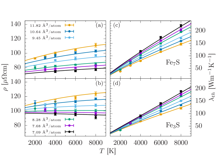
Figure 1: Electronic transport properties of liquid Fe–S alloys as a function of temperature. The temperature coefficient of electrical resistivity of liquid Fe₇S (a) and Fe₃S (b) decreases with compression due to saturation. For Fe₃S, the temperature coefficient of resistivity becomes negative along the smallest $V$ isochores. Solid lines represent the best fit of equation (7) to resistivity. Panels (c) and (d) show the electronic contribution to thermal conductivity of liquid Fe₇S and Fe₃S respectively. Solid lines have been calculated from the best fits to $\rho(V,T)$ (equation 7) and the effective Lorenz number $L(V,T)$ (equation 11). Tabulated values for $\rho$, $\lambda_{th}$ and $L$ are given in Tables S1 and S2 in the Supplemental Material.

Absolute resistivities for both compositions in the Fe-S system are similar to those for Fe-Si with the same light element concentration,(de Koker et al., 2012) and higher than those for pure Fe and in the Fe-O system.(de Koker et al., 2012; Pozzo et al., 2012) This is in contrast to experimental work(Suehiro et al., 2017) that estimated $\rho$ for the solid phase in a ternary Fe-Si-S system and calculated the S impurity resisitvity by using Matthiesen’s rule based on previous experimental results for Fe (Ohta et al., 2016) and Fe-Si.(Gomi et al., 2016) Suehiro et al. (2017) find that the influence of S on resistivity is significantly smaller than that of Si.(Gomi et al., 2016) The experiments had to rely on this indirect determination of resistivity reduction due to sulfur, as S is hardly soluble in solid Fe at ambient $P$ and it is therefore difficult to synthesize a homogeneous phase as a starting material in experiments.(Li et al., 2001; Stewart et al., 2008; Kamada et al., 2012; Mori et al., 2017) Further, Matthiesen’s rule, applied in the analysis of the data, does not hold for systems with saturated resistivity.(Gomi et al., 2016)

For higher sulfur concentration, we find that $\rho$ increases (Figure 1, cf. Figure S2 in the Supplemental Material) and that the Bloch-Grüneisen behavior breaks down. The temperature coefficient of resistivity decreases with compression, up to the extreme case where it changes sign and becomes negative for Fe₃S at the smallest two volumes we consider.

Negative TCR have been observed for liquid and amorphous solid metals, for which the maximum momentum change of a scattered electron $2k_{F}$ falls in the region close to the principle peak of the structure factor $S(q)$, as in case of metals with two valence electrons, e.g., Eu, Yb and Ba with a 6$s^{2}$ valence configuration,(Güntherodt et al., 1976) and Cu-Zr metallic glasses.(Waseda and Chen, 1978) It is one of the great successes of Ziman theory for the resistivity of liquid metals (Ziman, 1961; Faber and Ziman, 1965) to explain the negative TCR in these systems. Ziman theory can not account for the negative TCR that we predict for Fe₃S at high compression. As for iron and the other Fe-alloys considered by de Koker et al. (2012), $2k_{F}$ is near the first minimum in $S(q)$ (Figure S3 in the Supplemental Material), thermal broadening of the structure factor will lead to positive TCR over the entire compression range. This suggests that the negative TCR is a secondary effect, driven by changes in electronic structure (Section III.3) that is only noticable once resistivity saturation is reached by compression and impurities simultaneously.

III.2 Mean free path

In order to understand the effect of resistivity saturation from a semi-classical picture of electron transport, we calculate the effective electron mean free path as $x_{\mathrm{eff}}=v_{F}\tau$, where $v_{F}=(\hbar/m)\cdot(3\pi^{2}n_{\mathrm{eff}})^{1/3}$ is the Fermi velocity, $n_{\mathrm{eff}}=(m\sigma_{0})/(e^{2}\tau)$ the effective number density of conduction electrons and $m$ the electron mass. Figure 2 reveals three distinctive features:

(i) For ambient $P$ volumes ($V=11.82$ ų/atom), $x_{\mathrm{eff}}$ approaches the mean interatomic distance asymptotically with increasing $T$, consistent with dynamic resistivity saturation.(Mooij, 1973; Pozzo and Alfè, 2016)

(ii) At the lowest cell $V$ considered ($V=7.09$ ų/atom), the $T$-dependence of $x_{\mathrm{eff}}$ vanishes within uncertainty. In addition, $x_{\mathrm{eff}}$ becomes shorter than at lower compression due to the increased density of scattering centers. At first glance, this observation appears to be inconsistent with the fact that $\rho$ decreases with compression, but can be understood in terms of electronic structure (Section III.3).

(iii) With increasing sulfur concentration, $x_{\mathrm{eff}}$ decreases significantly. This reflects the expected behavior of an increased probability of impurity-caused scattering.

For the highest compression the Ioffe-Regel condition is reached for Fe₃S as $x_{\mathrm{eff}}$ becomes equal to the mean interatomic distance within uncertainty.

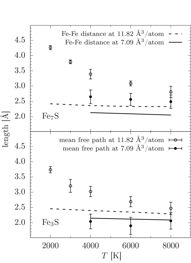
Figure 2: Electron mean free path for liquid Fe₇S (top) and Fe₃S (bottom) for two cell volumes (near ambient $P$ and largest compression) as a function of temperature, obtained by a Drude-fit to optical conductivity (equation 6). The mean free path approaches the interatomic distance (solid lines, first peak position of the partial radial distribution function) with increasing compression and impurity concentration. For Fe₃S at the smallest cell volume, the Ioffe-Regel condition is reached.

III.3 Electronic structure

Most of the electric current in transition metals is transported by $s$-electrons, which can scatter into $d$-states with a far lower Fermi velocity.(Mott, 1936) Partially filled $d$-bands with a high DOS at the Fermi level lead to a high probability of $s$-$d$ scattering events, which dominate resistivity over $s$-$s$ processes.(Mott, 1972)

Site-projected and angular momentum-decomposed densities of states (LDOS) show similar changes in response to compression and $T$ (Figures S4 and S5 of the Supplemental Material). Generally, peaks broaden and the Fe $d$-LDOS at $E_{F}$ decreases, resulting in fewer states available for $s$-electrons to scatter into. The response of the electronic structure to compression is a dominant feature as dispersion of electronic bands increases significantly due to stronger interactions (Figure S4 in the Supplemental Material).(Cohen et al., 1997)

For increasing $T$, changes in the DOS are less pronouced (Figure S5 in the Supplemental Material) and reflect dynamic short range changes in the liquid structure that can lead to smaller interatomic distances(Hunt et al., 2003) that is also expressed by thermal pressure.(Pozzo and Alfè, 2016) This is a small effect, and the negative TCR can only be observed when compression and chemical saturation in the system has been reached.

Electronic states of iron dominate the DOS of the liquid Fe-S alloys near $E_{F}$. The densities of states for Fe and Fe₃S are quite similar at the same $V$ and $T$ (Figures S4 and S5 in the Supplemental Material) and the broadening in the vicinity of $E_{F}$ due to compression and $T$, respectively, is almost identical. Therefore, sulfur contributes to the overall resistivity behavior in the Fe-S systems only by shortening $x_{\mathrm{eff}}$ through impurity scattering as discussed in Section III.2 (Figure 2). In comparison to silicon and oxygen, sulfur appears to be more efficient in doing so due to its similar atomic size and the efficient bonding with iron, resulting in high Fe-S coordination numbers. (Alfè and Gillan, 1998)

III.4 Thermal conductivity

Since lattice vibrations play only a minor role in heat transport through metals, the electronic contribution to thermal conductivity $\lambda^{el}_{th}$ represents total conductivity $\lambda_{th}$ to a good approximation. (Ashcroft and Mermin, 1976) Similar to the results for $\rho$, we find the Kubo-Greenwood values for $\lambda_{th}$ (Figure 1) to be consistent with the ones of liquid Fe-Si alloys, and somewhat larger than those of Fe-O liquids from previous computations with the same light element concentrations.(de Koker et al., 2012) Contrary to electrical resistivity, we do not see any sign of saturation in $\lambda_{th}$, putting the validity of the Wiedemann-Franz law with a constant value of the Lorenz number $L_{0}\approx 2.44$ W$\Omega$/K² from Drude-Sommerfeld theory in question. Indeed, thermal conductivity is significantly overestimated by using $L_{0}$ and the the resistivity model (Appendix A) compared to the values computed directly with the Kubo-Greenwood equations (equation 5).

Recently, electron-electron scattering has been suggested to contribute significantly to $\lambda_{th}$ of hcp iron at high $P$, but not to $\rho_{el}$,(Pourovskii et al., 2017) an effect that is ignored in the independent electron approximation of the Kubo-Greenwood approach. However, it remains an open question to what degree this contribution affects thermally disordered systems. Electronic transport critically depends on the electronic structure at the Fermi level, which is quite different for a high density liquid at high $T$, compared to a perfect crystal. Until the influence of electron-electron scattering on transport properties of disordered $3d$ transition metals and their alloys is better understood, values for $\lambda_{th}$ from the Kubo-Greenwood approach should be used with caution.

III.5 Application to planetary interiors

We convert resistivity values and fits in $V$-$T$ space (Appendix A and Table 1) to $\rho(P,T)$ by using the self-consistently obtained equations of state for Fe₇S and Fe₃S (Appendix B, Figure S6 and Table S3 in the Supplemental Material). Resistivity values for Fe₇S and Fe₃S (Figure 3) are substantially larger than the corresponding ones for pure iron. While resistivities for Fe₇S along different isotherms continue to show distinctive $P$-trends, they become indistinguishable for Fe₃S at high $P$ due to the combined saturation effects discussed in Section III.2. For Fe₃S, resistivity saturates at $\sim$100 $\mu\Omega$cm, a value which remains approximately constant and $T$-independent over the $P$-range of the Earth’s outer core, similar to the behavior of Fe₃Si.(de Koker et al., 2012)

Figure 3: Electrical resistivity of liquid Fe–S alloys as a function of pressure for Fe₇S (top) and Fe₃S (bottom). Solid lines are best fits of a parallel resistor model to $\rho(V,T)$ (equation 7) converted from $V$-$T$ to $P$-$T$ conditions using the equation of state fits (Appendix B). Results from an experimental study (Suehiro et al., 2017) along a model areotherm (red line) and geotherm (blue line) as well as computational results for pure Fe (de Koker et al., 2012) between 2000 and 8000 K (gray area) are included for comparison.

There is a large discrepancy between our results and the high $T$ extrapolation of experimental resistivity,(Suehiro et al., 2017) reported along model adiabats in the cores of Mars and the Earth.(Fei and Bertka, 2005; Kamada et al., 2012) Despite the similar composition between the work presented here and the experiments (that fall between Fe₃S and Fe₇S, towards the higher sulfur concentration), the experimental profile for Earth’s core shows significantly lower values, more consistent with the Kubo-Greenwood results for pure Fe.(de Koker et al., 2012; Pozzo et al., 2012) Model values of Suehiro et al. (2017) in the $P$-range of the Martian core are closer to our results (Figure 3), but the slope $(\partial\rho/\partial P)_{S}$ in the model based on experiments is significantly larger than in our work.

A small contribution to the difference between the experimental data and our results may come from the fact that the experiments have been performed for the solid and the simulations on the liquid, and resistivity increases discontinuously across the melting point for metals and their alloys both at ambient(Rosenfeld and Stott, 1990) and high $P$.(Secco and Schlössin, 1989; Silber et al., 2017; Ezenwa and Secco, 2017; Ezenwa et al., 2017) However, based on the Ziman approximation,(Ziman, 1961) this difference is expected to decrease with $P$ if density and compressibility of the coexisting solid and liquid phases become more similar. For pure iron, for example, this discontinuity is likely to become negligible at conditions of the Earth’s core.(Wagle and Steinle-Neumann, 2018) Rather than the difference decreasing with $P$ as expected, it increases between the experimental data(Suehiro et al., 2017) and our computational results (Figure 3).

IV Conclusions

We present electronic transport properties of liquid Fe-S alloys from DFT-MD simulations at conditions relevant for the cores of terrestrial planets. We find absolute values of electrical resistivity and thermal conductivity to be consistent with those of other Fe-light element alloys reported in previous work, (de Koker et al., 2012; Pozzo et al., 2014) ranging from 75 to 125 $\mu\Omega$cm and 30 to 220 Wm^-1K^-1. Fe alloys with low S content exhibit a positive TCR along isochores, which gradually decreases upon compression. We show that this is due to a compression-induced resistivity saturation by comparing the electron mean free path to interatomic distances. For high S concentrations (Fe₃S), the mean free path is further shortened by increased impurity scattering, sufficient to reach the Ioffe-Regel condition at the lowest volumes, resulting in a saturation of resistivity. At these conditions the TCR becomes negative which is caused by a decrease of the Fe $d$-density of states at the Fermi level.

For applications in planetary physics, we provide models for $\rho(V,T)$ and $\lambda_{th}(V,T)$ (Appendix A), which, in combination with a self-consistent thermodynamic equation of state (Appendix B), can be translated to $P$-$T$ conditions of planetary cores.

Appendix A Model for electrical and thermal conductivity

We describe the resistivity behavior $\rho(V,T)$ by a parallel resistor model:

$$\frac{1}{\rho(V,T)}=\frac{1}{\rho_{BG}(V,T)}+\frac{1}{\rho_{sat}(V)}+\frac{1}{\rho_{el}(T)},$$ (7)

where

$$\rho_{BG}=\rho_{0}\left(\frac{V}{V_{0}}\right)^{a}+\rho_{1}\left(\frac{V}{V_{0}}\right)^{b}\frac{T}{T_{0}}$$ (8)

is the empirical expression used by de Koker et al. (2012) based on the Bloch-Grüneisen formula.

$$\rho_{sat}=c\left(\frac{V}{V_{0}}\right)^{\frac{1}{3}}$$ (9)

is a term accounting for resistivity saturation and

$$\rho_{el}=d\frac{T_{0}}{T}$$ (10)

describes the effect of thermal broadening of the DOS. The assumptions entering equations (7)–(10) are:

(i) Sources of resistivity contributions in equation (7) are independent and therefore conductivities are additive.

(ii) In the limit of high $T$, the Bloch-Grüneisen formula is linear in $T$. Both residual resistivity (first term in equation 8) and the material dependent prefactor of the second term are well described by a power law in $V/V_{0}$.

(iii) Saturation resistivity (equation 9) is proportional to interatomic distance and therefore increases $\propto\left(V/V_{0}\right)^{1/3}$. This is consistent with saturation resistivities for pure Fe reported by Ohta et al. (2016)

(iv) Since the effect of thermal broadening on the DOS at $E_{F}$ can be attributed to a resistivity contribution due to thermal pressure (Figure S5 in the Supplemental Material), we describe $\rho_{el}$ in equation (10) as inversely proportional to $T$.

Rather than fitting a model for $\lambda_{th}$ directly, we compute an effective Lorenz number $L$ at each simulation and fit the $L(V,T)$ as(de Koker et al., 2012)

$$L(V,T)=L_{R}\left(\frac{V}{V_{0}}\right)^{e}\left(\frac{T}{T_{0}}\right)^{f}.$$ (11)

Fit parameters are listed in Table 1.

Table 1: Fit parameters of the models for $\rho(V,T)$ (equations 8–10) and $L(V,T)$ (equation 11) for liquid Fe, Fe₇S and Fe₃S. Uncertainties of the fit parameters are large and exceed their values in most cases.

		Fe	Fe7S	Fe3S
$\rho_{0R}$	[$\mu\Omega$cm]	75.10	89.03	105.2
$\rho_{1R}$	[$\mu\Omega$cm]	21.48	12.73	12.06
$a$		0.792	0.389	0.124
$b$		1.479	1.804	2.686
$c$	[$\mu\Omega$cm]	747.2	2077	6609
$d$	[$\mu\Omega$cm]	1405	2829	2910
$L_{R}$	[W$\Omega$/K2]	2.005	2.105	1.991
$e$		-0.097	-0.106	-0.228
$f$		0.041	-0.027	-0.022

Appendix B Equation of state model

In order to describe electronic transport properties as a function of $P$, suitable for comparison to experiments and for applications in planetary models, we fit a thermodynamic model to the Fe₇S and Fe₃S results that is based on an separation of the Helmholtz energy in an ideal gas, electronic and excess term.(de Koker and Stixrude, 2009; Vlček et al., 2012) The volume dependence of the excess term is represented by Eulerian finite strain ($f$) with exponent $n=2$ and a similarly reduced $T$-term ($\Theta$) with exponent $m=0.79$ and expansion orders $\mathcal{O}_{f}=3$ and $\mathcal{O}_{\Theta}=2$, parameters that describe the results for liquid iron well.(de Koker et al., 2012) Figure S6 in the Supplemental Material shows the quality of the fit for $E$, $P$ and electronic entropy $S_{el}$ of the DFT-MD results. Thermodynamic parameters at reference conditions are summarized in Table S3 of the Supplemental Material.