Relational Quantum Mechanics and Probability

Abstract

We present a derivation of the third postulate of Relational Quantum Mechanics (RQM) from the properties of conditional probabilities. The first two RQM postulates are based on the information that can be extracted from interaction of different systems, and the third postulate defines the properties of the probability function. Here we demonstrate that from a rigorous definition of the conditional probability for the possible outcomes of different measurements, the third postulate is unnecessary and the Born’s rule naturally emerges from the first two postulates by applying the Gleason’s theorem. We demonstrate in addition that the probability function is uniquely defined for classical and quantum phenomena. The presence or not of interference terms is demonstrated to be related to the precise formulation of the conditional probability where distributive property on its arguments cannot be taken for granted. In the particular case of Young’s slits experiment, the two possible argument formulations correspond to the possibility or not to determine the particle passage through a particular path.

1 Introduction

After more than 100 years from the first attempt to formulate Quantum Mechanics (QM) by postulates Bohr1913 , its interpretation and foundation are still in discussion in the scientific community. The origin of this open issue partially lies in the fact that our process of understanding is strongly based on the ability to make analogies with something familiar to us. In the case of quantum phenomena, this approach fails because in our daily environment these kinds of events are not evident. In the Young’s slit experiment for example, where a massive particle or photons pass through the slits and form an interference pattern on a screen, we compare this phenomenon to common systems such as a ping-pong ball or sea waves. The non-compatibility and contradictions between these two analogies create the impression to deal with paradoxes producing a sense of discomfort. This difficulty to deal with quantum phenomena is well manifested by the famous phrase of R. Feynman who, in his sixth lecture The character of physical law at Cornell University in 1964 Feynman1967 , provocatively stated “I think I can safely say that nobody understands quantum mechanics”. Without going into the discussion of the meaning of understanding, different interpretations of quantum phenomena and different choices of QM postulates can be discussed. Several approaches have been formulated since the early days of Quantum Mechanics and have been amply discussed in the literature (see e.g. Ref. Auletta and references therein). New approaches and interpretations continue to be proposed Hardy2001 ; Clifton2003 ; Grinbaum2007 ; Grinbaum2007a ; Dakic2009 ; Hohenberg2010 ; Chiribella2011 ; Fuchs2013 ; Masanes2013 ; Barnum2014 ; Dickson2015 ; Auffeves2016 ; Friedberg2018 demonstrating a strong interest in this subject still nowadays.

To choose among the different QM interpretations and postulates formulations, a pragmatic approach is to consider two important criteria (i) the simplicity of the theory, following the Ockham’s razor philosophical principle, and (ii) an interpretation that uses as ingredients for the postulates formulation, the concepts that are most familiar to our common experience. To satisfy this second criterion, a way chosen by many authors in recent years is to use as basis of interpretations or foundation of QM the information that can be exchanged between the system and another system or an observer Rovelli1996 ; Brukner1999 ; Brukner2002 ; Fuchs2002 ; Clifton2003 ; Barrett2007 ; Brukner2009 ; Dakic2009 ; Chiribella2011 ; Masanes2013 ; Hohn2017 ; Hohn2017a ; Hohn2017b ; Yang2017 ; Yang2018 ; Yang2018a . The first postulation of QM in terms of information is due to Rovelli in 1996 with the formulation of Relational Quantum Mechanics (RQM) Rovelli1996 ; Smerlak2007 ; Rovelli2018 . In RQM framework, no system is privileged (there is no observable and observer, both are considered simply different systems) and everything depends on the reciprocal relationship through the mutual interaction, hence the name “Relational” in RQM. The aspect of the quantization of nature is dictated in the first postulate by imposing a maximum limit on the information that can be extracted from a system. The probabilistic aspect of the theory is introduced by the second postulate that states that, even when all possible information is available, new one can be extracted from a system. The third and last postulate, less intuitive, defines the way to compute probabilities, imposing, accordingly to experimental observations (Young’s slits for ex.), the calculation via squares of amplitudes and sums of amplitudes (Born’s rule). In the context of RQM, new developments and discussions appeared in the last years Poulin2006 ; Grinbaum2007 ; Grinbaum2007a ; Brown2009 ; vanFraassen2009 . In particular, EPR-type experiment have been reinterpreted in the context of RQM Smerlak2007 , it has been demonstrated that properties of orthmodularity are a direct consequence of the first two postulates of RQM Grinbaum2005 and, very recently, an alternative reconstruction of the Hilbert space is derived from the first two RQM postulates and four additional postulates Hohn2017 ; Hohn2017a ; Hohn2017b .

In this article we present a derivation of the third postulate of RQM from the first two postulates and the basic properties of conditional probability function. In the original article of RQM Rovelli1996 , Rovelli writes

“One could conjecture that equations (13)–(17) (the equations relatives to probability properties, N.A.) could be derived solely by the properties of conditional probabilities …Here, I content myself with the much more modest step of introducing a third postulate.”

The main result presented here is exactly to demonstrate Rovelli’s conjecture from first principles, thus eliminating the need of introducing a third postulate. We will demonstrate in particular that, when the most general probability function is rigorously defined, Born’s rule emerges from the first two RQM postulates by the use Gleason’s theorem. The approach presented here is alternative to the recent work from Höhn Hohn2017 ; Hohn2017a ; Hohn2017b of QM foundation from the first two RQM postulated and additional ones. Differences between the two methods and their corresponding assumptions will be discussed.

To present how to apply the developed formalism in a concrete case, we will consider the example of Young’s slits experiment and we will calculate probabilities in cases of distinguishability or indistinguishability of the particle path through the slits pair. We will in particular demonstrate that the probability function is uniquely defined for both cases. The presence or not of interference terms is related to the precise formulation of the conditional probability where distributive property on its arguments cannot be taken for granted.

The article is organized as follows: in Sec. 2, as introduction, we present the first two RQM postulates and their relation to the measurement processes and Hilbert spaces. In Sec. 3 we discuss how we can built a probability function and we will study its properties. Section 4 analyses the Young’s slits experiment in the framework of the formalism developed. We will end the article with the sections of conclusions (Sec. 5) and an appendix for an introduction to orthomodular lattices and their connections with “yes/no” experiments.

2 An introduction to Relational Quantum Mechanics: postulates, measurements algebra and Hilbert space

This chapter is an introduction with some examples of RQM postulates. In particular, we recall here past major results on the theory of lattices associated to “yes/no” experiments and the reconstruction of the Hilbert space in the context of RQM.

2.1 Interacting systems and measurement processes

The basic assumption of RQM is that the world can be decomposed into a collection of systems, each of which can be equivalently considered as an observing system or as an observed system. The information is exchanged via physical interaction between systems. The process of acquisition of information can be described as a “question” that a system (observing system) asks another system (observed system). Since information is discrete, any process of acquisition of information can be decomposed into acquisitions of elementary bits of information by a series of “yes/no” experiment, i.e. a click or not of a specific measurement apparatus.

On another hand, a set of “yes/no” measurements on a same system preparation can be seen as a set of propositions linked to each other by an ordered relationship “$\succeq$” Birkhoff1936 ; VonNeumann ; BeltramettiCassinelli ; Hughes . If $i,j$ represent two possible measurement results, the relationship $i\succeq j$ indicates that each time we have a certain yes outcome for $j$ also we have a certain yes outcome for $i$. The ensemble of propositions and the order relation between them form a structure called partially ordered set (poset) with some particular properties (orthocomplementation and other properties) that will be essential to define from it a Hilbert space.

It is not the intent of this article to make an introduction to poset and orthocomplemented lattices. Here we will present only their basic properties in the relation with RQM postulates. For the readers that are not familiar to these structures, their properties and their connection to “yes/no” measurements of classical and quantum phenomena, a short introduction is presented in the appendix at the end of the article. An exhaustive presentation on this topic can be found in Refs. BeltramettiCassinelli ; Hughes .

2.2 First postulate of RQM and orthocomplemented lattices

The first postulate of RQM is Rovelli1996

Postulate 1 (Limited information): there is a maximum amount of relevant information that can be extracted from a system.

If there is a maximal amount of information that can be extracted from the system, it exists an ensemble of $N^{\prime}$ questions $Q^{i}$ that completely describes the system. These questions can be represented by different experimental results: the detection of a particle with spin up or down or the measurement of a particle momentum within a value interval. If the information is limited, this means that exists a list of limited “yes/no” questions $Q^{i}$ with $i=1,\ldots N\leq N^{\prime}$ independent from each other that describes completely the system. With the operations of conjunction “$\land$” (“AND”), disjunction “$\lor$” (“OR”) and negation “$\lnot$” (“NOT”), we can in addition build another list of mutually exclusive questions $Q_{\alpha}^{i}$ where $Q_{\alpha}^{i}\land Q_{\alpha}^{j}=\emptyset$ for $i\neq j$ Rovelli1996 , where the Greek letter indicate belonging to the same complete set of questions and “$\emptyset$” defines an empty set. For each pair of questions, the combinations $Q_{\alpha}^{i}\land Q_{\alpha}^{j}$ and $Q_{\alpha}^{i}\lor Q_{\alpha}^{j}$ are univocally defined. Because we have a complete set of questions, we have that $\bigvee_{i}Q_{\alpha}^{i}=\mathbb{1}$, the ensemble of all possible positive answers, defines certainty (represented here by “$\mathbb{1}$”).

For each question $Q_{\alpha}^{i}$ (e.g. “is the spin up?”) its positive answer correspond to a statement $i$ (“the spin is up”). A negative answer corresponds to its complementary statement $i^{\bot}$ (“the spin is not up”), which correspond to a positive answer to the question $\lnot Q_{\alpha}^{i}$ opposite to $Q_{\alpha}^{i}$. The different possible answers $\{i,i^{\bot}\}$ together with the operations “$\land$”, “$\lor$” constitute a logical structure called lattice, indicated by $\mathcal{L}$. This lattice is orthocomplemented because for each element $i$ (a positive answer), it exist is complement $i^{\bot}$ (a negative answer to the same question), with the properties $i\lor i^{\bot}=\mathbb{1}$ and $i\land i^{\bot}=\emptyset$, where $\mathbb{1},\emptyset$ are also part of the lattice $\mathcal{L}$ (a complete lattice).

Another important property of the lattice defined by a complete series of mutually exclusive questions is the distributivity, which corresponds to the property

$$i\land(j\lor k)=(i\land j)\lor(i\land k),\quad i\lor(j\land k)=(i\lor j)\land(i\lor k)$$ (1)

for any triplet $i,j,k\in\mathcal{L}$. As we will see in the following sections where we will consider more than one set of complete questions, distributivity, or more precisely its absence, will play an important role to calculate interference phenomena in the probability calculation. Note, a distributive orthocomplemented lattice is also called Boolean lattice.

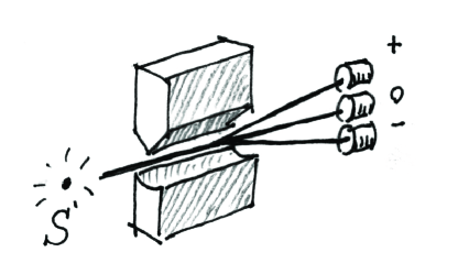
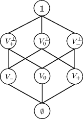
Figure 1: Left: artistic scheme of a Stern-Gerlach experiment with vertically aligned magnets. Right: graph of the orthocomplemented lattice corresponding to the detection of the three emerging beams.

A simple example of a complete set of questions can be built considering a spin-1 particle passing through a Stern-Gerlach apparatus with a defined axis orientation, vertical for example (see Fig. 1 left). Here the spin orientation of the particle is determined by the deflection of the particle itself passing through a non-homogeneous magnetic field. The complete set of question is constituted by a series of three particle detectors that correspond to the questions $\{Q_{V}\}=Q_{V}^{+},Q_{V}^{0}$ and $Q_{V}^{-}$, one for each spin projection. The ensemble of the corresponding answers $\{V_{+},V_{0},V_{-},V^{\bot}_{+},V^{\bot}_{0},V^{\bot}_{-}\}$ forms a orthocomplemented distributive (Boolean) lattice represented in Fig. 1 right (see Appendix for more details on lattices properties).

From the output of the three detectors we can extract only a limited amount of information. In opposite, in a classical case as the measurement of egg holes by different calibers (see Appendix), from the use of additional holes with different diameters, additional information can be always be extracted.

2.3 Second postulate of RQM and orthomodular lattices

The second postulate of RQM is Rovelli1996

Postulate 2 (Unlimited questions): it is always possible to acquire new information about a system.

When a particle coming out from a Stern-Gerlach apparatus, vertically oriented for example, is injected into another Stern-Gerlach apparatus with a different orientation, e.g. horizontal, the new output can be used to extract new information with a loss of old information because its total quantity is bounded. The new results $\{H_{+},H_{0},H_{-},H^{\bot}_{+},H^{\bot}_{0},H^{\bot}_{-}\}$ correspond to a new set of questions $\{Q_{H}\}=Q_{H}^{+},Q_{H}^{0},Q_{H}^{-}$.As for the vertical case, the new possible outcomes alone have a mutual relation similar to the scheme in Fig. 1 (right). But when horizontal and vertical measurement apparatus are not considered subsequentially but together as alternative measurements, they form a lattice that is no more distributive, contrary to classical cases as a egg measured by two different sets of calibers (see Appendix).

The non-distributivity of the lattice is related to the fact that each set of questions is complete, but the sets are not compatible each other because each apparatus can extract an information $I_{\text{max}}$ and the maximal quantity of information that can be extracted is also $I=I_{\text{max}}$. The absence of the distributive property has major consequences. It implies in fact that the order on which the questions/measurements are made matters and is related to the commutation of operators in standard QM.

As pointed in the early years of QM Birkhoff1936 , proposition lattices defined by set of measurements of classical or quantum cases, have still in common an important property, orthomodularity, which is a weaker property than distributivity consisting in

$$i=j\lor(i\land j^{\bot})$$ (2)

for each pair of elements $i,j\in\mathcal{L}$ with $i\succeq j$. Recently, Grinbaum demonstrated Grinbaum2005 that orthomodularity property is in fact a direct consequence the presence of upper bound of information. To note that for this demonstration the author introduces the property of relevance between pairs of questions. This property can be used to discriminate questions belonging to the same complete set or to different sets.

A final comment to the second postulate is that it can be actually considered, as a lower bound on the information, in complement to the first postulate that determine the higher bound. Absolute certainty corresponds to a zero information gain. Postulate 2 of RQM assure that we can extract always information larger than zero.

2.4 Reconstruction of the Hilbert space

It has been demonstrated that if we have an orthomodular lattice $\mathcal{L}$, which is in addition atomic, complete and has covering property, an Hilbert space $\mathcal{H}$ can be reconstructed BeltramettiCassinelli ; Auletta ; DallaChiara . As discussed above, orthomodularity can be derived directly from the first two RQM postulates Grinbaum2005 . Similarly, completeness is directly derived by construction of RQM because a system can be completely described by a finite number of answers of “yes/no” questions due to the information boundaries. Moreover, each question constitutes actually an atom of the lattice $\mathcal{L}$. The covering property, valid for many lattices corresponding to measurements of quantum systems, has to be assumed valid the general case for the reconstruction of $\mathcal{H}$ (on this assumption we will discuss more extensively in the next paragraphs). Even if the Hilbert space $\mathcal{H}$ is reconstructed from the lattice formed by complete sets of questions, the choice of its numbered field (real, complex, quaternion, p-adic, etc. ) is not defined. However, it can be demonstrated that the complex case satisfies the basic requirements for describing quantum phenomena without redundancy BeltramettiCassinelli .

In the reconstruction of the Hilbert space from the orthomodular lattice, each complete set of questions $\{Q_{\alpha}^{i}\}$ is associated to a basis $\{\ket{i_{\alpha}}\}$ of $\mathcal{H}$. Moreover, from any $\ket{i_{\alpha}}$ we can built a projector $P^{i}_{\alpha}=\ket{i_{\alpha}}\bra{i_{\alpha}}$. Different sets of questions $\{\ket{i_{\alpha}}\},\{\ket{j_{\beta}}\}$ correspond to different complete bases that are related to each other via unitary matrices $U$ with $\ket{j_{\beta}}=U\ket{i_{\alpha}}$. The unitarity of $U$ is guaranteed by the completeness and orthogonality of each basis element Cohen . In this context, a pure state, $\ket{i_{\alpha}}$, correspond to a certain positive answer to a question of a complete set. A mixed state is the results of an uncertainty between answers of among questions.

3 Probability function and properties

3.1 Definition of probability function

Taking into account two complete families of questions $\{Q_{\alpha}^{i}\},\{Q_{\beta}^{j}\}$ and the second RQM postulate, we can consider the probability for obtaining a positive answer to the question $Q_{\beta}^{j}$ knowing a positive answer to the question $Q^{1}_{\alpha}$. This is a perfect example of conditional probability that can be indicated by $p[Q_{\beta}^{j}|Q_{\alpha}^{i}]$. In the next paragraphs we will build $p[Q_{\beta}^{j}|Q_{\alpha}^{i}]$ from minimal requirements for the most general definition of probability function.

In its most general definition, probability is a measurement or map on a set of elements $\Omega$ to the real interval $[0,1]$ via a function $\wp:\Omega\to[0,1]$ SEPprob ; Fine . The first axiomatization of the probability function $\wp$ is due to Kolmogorov in 1933 Kolmogorov ; Fine ; Jaynes where $\Omega$ is on a field $\mathcal{F}$ that is closed under complementation with respect to $\Omega$ and union and where

$$\wp[A]\geq 0\text{ for all $A\in\mathcal{F}$},$$ (3a)

$$\wp[\Omega]=1,$$ (3b)

$$\wp[A\cup B]=\wp[A]+\wp[B]\text{ for all $A$ and $B\in\mathcal{F}$ with $A\cap B=\emptyset$}.$$ (3c)

This general form is normally implemented in different cases of classical or quantum physics Fine ; Gudder ; Varadarajan ; Hughes ; Auletta ; DallaChiara and is more or less explicitly used in all approaches of foundations of QM.

In the context of logic of $True/False$ values of sentences of a set $\mathcal{S}$, an analog definition of $\wp$ is SEPprob ; Cox ; Fine

$$\wp[A]\geq 0\text{ for all $A\in\mathcal{S}$},$$ (4a)

$$\wp[\text{{True}}]=1,$$ (4b)

$$\wp[A\land B]=\wp[A]+\wp[B]\text{ for all $A$ and $B\in\mathcal{S}$ with $A\land B=\emptyset$}.$$ (4c)

This is a more adapted set of axioms of $\wp$ to be directly implemented for probability measurements in orthomodular lattices $\mathcal{L}$ BeltramettiCassinelli and RQM where sentences of $\mathcal{S}$ are positive or negative answers of questions.

To correctly define the probability function $p[Q_{\beta}^{j}|Q_{\alpha}^{i}]$ for obtaining a positive answer to a question $Q_{\beta}^{j}$ knowing a positive answer to a question of another family $Q_{\alpha}^{i}$, we have to introduce conditionality properties. To underline that we are dealing with measurements that corresponds to answers to questions, in the previous expression and in the following paragraphs we implicitly indicates by $Q^{i}$ its corresponding positive answer and $\lnot Q^{i}\equiv Q^{i^{\bot}}$ the corresponding negative answer. Taking inspiration from Refs. Ballentine1986 ; Fine ; Jaynes ; Ballentine2016 , from Eqs. (4) we can derive the axioms

$$p[Q_{\beta}^{j}|Q_{\alpha}^{i}]\geq 0,$$ (5a)

$$p\Big{[}\bigvee_{j}Q_{\beta}^{j}\Big{|}Q_{\alpha}^{i}\Big{]}=1,$$ (5b)

$$p[Q_{\beta}^{j}\lor Q_{\beta}^{k}|Q_{\alpha}^{i}]=p[Q_{\beta}^{j}|Q_{\alpha}^{i}]+p[Q_{\beta}^{k}|Q_{\alpha}^{i}],$$ (5c)

for the probability relative to the set of questions $Q_{\beta}^{j}$ knowing a positive question $Q_{\alpha}^{i}$. The second axiom states that the probability of certainty is 1. It corresponds to Eqs. (3a) and (4a), and it is equivalent to $p[Q_{\beta}^{j}|Q_{\beta}^{j}]$ =1. Because of the completeness of each set of questions, we have in fact $\bigvee_{j}Q_{\beta}^{j}\equiv\mathbb{1}$, i.e. always True. Due to the mutual exclusivity of the questions $Q_{\beta}^{j}\land Q_{\beta}^{k}=\emptyset$ for $j\neq k$, Eq. (5c) is equivalent to Eq. (4c).

Similar definitions of conditional probability are implemented in the recent approach of QM foundation of Auffèves and Grangier Auffeves2016 ; Auffeves2017 and of Höhn Hohn2017 ; Hohn2017a ; Hohn2017b with however some important differences. Höhn assumes additional symmetric properties of $p$ (see next paragraphs) to reconstruct QM framework. This is not the case for Auffèves and Grangier where however the probability function is not rigorously defined, similarly to the case of RQM original formulation Rovelli1996 .

For a given answer of the question $Q_{\alpha}^{i}$ the probability function $p[\cdot|Q_{\alpha}^{i}]$ defined by Eqs. (5) is compatible with Kolmogorov’s axiomatic definition (Eqs. (3)). Differently from Kolmogorov approach, we will see that the explicit dependency on the prior answers provides a clear use of $p$ in different contexts.

3.2 The Gleason’s theorem and the third principle of RQM

In the previous sections we saw that from the first and the second postulates of RQM we can build a Hilbert space. This reconstruction enable to make a direct link to the different choices of probability axioms, Eqs. (3) and (5) and then the use of Gleason’s theorem Gleason1957 . Gleason’s theorem (from an adaption of Refs. Auletta ; BeltramettiCassinelli ) states:

In a separable Hilbert space $\mathcal{H}$ of dimension $\geq 3$, whether real, complex or quaternion, every probability measure (that respects Eqs. (3), N.A.) on a closed subspace $\mathcal{H_{S}}$ can be written in the form

$$p[H_{S}]=tr[\rho P_{\mathcal{S}}],$$ (6)

where $P_{\mathcal{S}}$ denotes the orthogonal projection on $\mathcal{H_{S}}$ and $\rho$ is a density operator.

In our notation a pure state $\ket{i_{\alpha}}$ corresponds to a certain positive answer to a question $Q_{\alpha}^{i}$ and it is associated to the density matrix $\rho_{\alpha}=\ket{i_{\alpha}}\bra{i_{\alpha}}$, which is in this case is equivalent to the projector $P^{i}_{\alpha}=\ket{i_{\alpha}}\bra{i_{\alpha}}$.

The probability for having a positive answer to the question $Q_{\beta}^{j}$ is

$$p[Q_{\beta}^{j}|Q_{\alpha}^{i}]=tr[\rho_{\alpha}P_{\beta}^{j}]=|\braket{j_{\beta}}{i_{\alpha}}|^{2}=|U_{ij}|^{2},$$ (7)

where $U_{ij}$ is the unitary matrix element corresponding to the transformation between the complete bases $\{\ket{i_{\alpha}}\}$ and $\{\ket{j_{\beta}}\}$ complete bases transformation and $P_{\beta}^{j}=\ket{j_{\beta}}\bra{j_{\beta}}$ is the projector corresponding to $Q_{\beta}^{j}$. Thus, we see that Born’s rule can be deduced solely from the first two RQM postulates and from Gleason’s theorem, without the need of any further assumption: a third postulate devoted to probabilities does not appear necessary.

From Eq. (7) we see that $p[Q_{\beta}^{j}|Q_{\alpha}^{i}]$ is completely symmetric to the exchange of order of the questions $Q_{\beta}^{j}$ and $Q_{\alpha}^{i}$,

$$p[Q_{\beta}^{j}|Q_{\alpha}^{i}]=p[Q_{\alpha}^{i}|Q_{\beta}^{j}],$$ (8)

a property that is only assumed as valid in the original formulation of RQM Rovelli1996 but also in the recent QM foundation approach from Höhn Hohn2017 ; Hohn2017a ; Hohn2017b and in other recent works.

From Eqs. (5), we have in addition the properties

$$p[\bigvee_{j}Q_{\beta}^{j}|Q_{\alpha}^{i}]=\sum_{j}p[Q_{\beta}^{j}|Q_{\alpha}^{i}]=\sum_{i}p[Q_{\alpha}^{i}|Q_{\beta}^{j}|]=p[\bigvee_{i}Q_{\alpha}^{i}|Q_{\beta}^{j}|]=1.$$ (9)

In other words $\sum_{i}|U_{ij}|^{2}=\sum_{j}|U_{ij}|^{2}=1$, which is one of the basic properties of unitary matrices Rovelli1996 ; Cohen .

3.3 Alternative foundations of QM via RQM postulates and discussion

In the previous section we demonstrated that from minimal requirements for the conditional probability function and the first two postulates of RQM, Born’s rule can be derived. It has to be noted that this demonstration is based on the assumption that any lattice $\mathcal{L}$ associated to quantum measurements has covering properties BeltramettiCassinelli ; Grinbaum2007 . This is the case for simple examples of simple quantum measurement graphs Birkhoff1936 ; Piron1972 ; Piron ; BeltramettiCassinelli ; Hughes but it is not proved for the general case. Here the cover property has to be assumed valid. Moreover, the numerical field of the Hilbert space cannot be derived from RQM principles and real and complex numerical fields are found only from a non-exhaustive exclusion of other cases. In particular the quaternion case is eliminated only when composite systems are considered BeltramettiCassinelli .

A recent alternative foundation of QM based on the first two principles of RQM, with addition of new postulates, has been proposed by Höhn Hohn2017 ; Hohn2017a ; Hohn2017b . In this remarkable work, real and complex numerical fields are deduced by construction from a set of five postulates: the first two RQM ones plus other three. The complex case becomes the only acceptable field once an additional postulate on the measurement of composite systems is added. This is a very interesting result but it has to be noticed that, in addition to the important increase of number of postulates where time coordinate has a preferential role, it relies on the additional assumption of the symmetric properties of the probability functions $p[Q^{i}|Q^{j}]$ with respect couple of questions $Q^{i},Q^{j}$. This is not the case in the demonstration proposed here were the symmetric properties of $p[Q^{i}|Q^{j}]$ are derived directly from Eq. (7). It interesting to note that in Höhn’s work, if the existence of a state of no information is assumed, $p[Q_{\beta}^{j}|Q_{\beta}^{j}]$ is used to classify families of questions, independent, dependent, partially dependent, similarly to the relation of relevance introduced by Grinbaum Grinbaum2005 between different lattice elements (see Sec. 2.3).

3.4 Additional properties of conditional probability function and Bayes’ theorem

Other non-trivial properties of the conditional probability function $p$ can be discussed considering three sets of complete questions. If we have three subsequent specific questions $Q_{\alpha}^{i},Q_{\beta}^{j},Q_{\gamma}^{k}$ from three different sets of complete questions, we can consider the probability $p[Q_{\gamma}^{k}|Q_{\beta}^{j}\ \rotatebox[origin={c}]{90.0}{$\geqslant$}\ Q_{\alpha}^{i}]$ for having a positive answer for $Q_{\gamma}^{k}$ knowing a positive answer for $Q_{\beta}^{j}$ after a positive answer for $Q_{\alpha}^{i}$. To take into account the order of the questions we introduce the new non-symmetric relation operator “ $\geqslant$ ”, similar to the “AND” logical operator “$\land$” but where $Q^{i}\ \rotatebox[origin={c}]{90.0}{$\geqslant$}\ Q^{j}\neq Q^{j}\ \rotatebox[origin={c}]{90.0}{$\geqslant$}\ Q^{i}$. We underline the importance of the sequence of the questions because it is related to the non-commutativity of the operators $P_{\alpha}^{i}$ and $P_{\beta}^{j}$, i.e. $P_{\alpha}^{i}P_{\beta}^{j}\neq P_{\beta}^{j}P_{\alpha}^{i}$. As we will see, when the sequence of the questions is not important, the operator “ $\geqslant$ ” reduces to the conjugation operator “$\land$”.

From Gleason’s theorem (Eq. (7)) and the properties of the density operator, and in particular Lüders’ rule for conditional probabilities, we have for pure states

$$p[Q_{\gamma}^{k}|Q_{\beta}^{j}\ \rotatebox[origin={c}]{90.0}{$\geqslant$}\ Q_{\alpha}^{i}]=\frac{tr[P_{\beta}^{j}\rho_{\alpha}P_{\beta}^{j}P_{\gamma}^{k}]}{tr[\rho_{\alpha}P_{\beta}^{j}]}=\frac{tr[P_{\beta}^{j}P^{i}_{\alpha}P_{\beta}^{j}P_{\gamma}^{k}]}{tr[P^{i}_{\alpha}P_{\beta}^{j}]}=\\ =\frac{tr[P_{\beta}^{j}P^{i}_{\alpha}P_{\beta}^{j}P_{\gamma}^{k}]}{p[Q^{i}_{\alpha}|Q_{\beta}^{j}]}=\frac{|\bra{k_{\gamma}}P^{j}_{\beta}\ket{i_{\alpha}}|^{2}}{|\braket{j_{\beta}}{i_{\alpha}}|^{2}}.$$ (10)

Because of the trace properties $tr[MNL]=tr[NLM]=tr[LMN]$ (but $\neq tr[MLN]$), the nominator of Eq. (10) is completely symmetric with respect to the interchange of $P^{i}_{\alpha}$ and $P^{k}_{\gamma}$. The difference between $p[Q_{\gamma}^{k}|Q_{\beta}^{j}\ \rotatebox[origin={c}]{90.0}{$\geqslant$}\ Q_{\alpha}^{i}]$ and $p[Q_{\gamma}^{k}\ \rotatebox[origin={c}]{90.0}{$\geqslant$}\ Q_{\beta}^{j}|Q_{\alpha}^{i}]$ is only the denominator,

$$p[Q_{\gamma}^{k}\ \rotatebox[origin={c}]{90.0}{$\geqslant$}\ Q_{\beta}^{j}|Q_{\alpha}^{i}]=tr[P_{\beta}^{j}P^{i}_{\alpha}P_{\beta}^{j}P_{\gamma}^{k}]=|\bra{k_{\gamma}}P^{j}_{\beta}\ket{i_{\alpha}}|^{2},$$ (11)

which is required for the probability normalisation. In other words, we have

$$p[Q_{\gamma}^{k}|Q_{\beta}^{j}\ \rotatebox[origin={c}]{90.0}{$\geqslant$}\ Q_{\alpha}^{i}]=\frac{p[Q_{\gamma}^{k}\ \rotatebox[origin={c}]{90.0}{$\geqslant$}\ Q_{\beta}^{j}|Q_{\alpha}^{i}]}{p[Q^{i}_{\alpha}|Q_{\beta}^{j}]},$$ (12)

which is very similar to Bayes’ theorem for conditional probability except for the presence of the operator “ $\geqslant$ ” instead of the conjunction “$\land$”.

If the projectors relative to questions commute additional simplifications can be applied BeltramettiCassinelli . In this case we have $P_{\beta}^{j}P_{\gamma}^{k}=P_{\gamma}^{k}P_{\beta}^{j}$ that, together with Eq. (10) gives

$$p[Q_{\gamma}^{k}|Q_{\alpha}^{i}\ \rotatebox[origin={c}]{90.0}{$\geqslant$}\ Q_{\beta}^{j}]=\frac{tr[P_{\beta}^{j}\rho_{\alpha}P_{\beta}^{j}P_{\gamma}^{k}]}{tr[\rho_{\alpha}P_{\beta}^{j}]}=\frac{tr[\rho_{\alpha}P_{\beta}^{j}P_{\gamma}^{k}]}{tr[\rho_{\alpha}P_{\beta}^{j}]}=\\ =\frac{p[Q_{\gamma}^{k}\land Q_{\beta}^{j}|Q_{\alpha}^{i}]}{p[Q_{\beta}^{j}|Q_{\alpha}^{i}]}\equiv p[Q_{\gamma}^{k}|Q_{\alpha}^{i}\land Q_{\beta}^{j}],$$ (13)

which is nothing else the Bayes’ theorem with “ $\geqslant$ ” equivalent to “$\land$”. We note that the demonstration of the Bayes’ theorem provided by Cox and Jaynes Cox1946 ; Jaynes is based on the assumption that the conditional probability $p[Q_{\gamma}^{k}\land Q_{\beta}^{j}|Q_{\alpha}^{i}]$ can be written as function of $p[Q_{\gamma}^{k}|Q_{\alpha}^{i}\land Q_{\beta}^{j}]$ and $p[Q_{\beta}^{j}|Q_{\alpha}^{i}]$ Cox1946 ; Fine ; Jaynes . This is clearly not true for the general case described by Eq. (10) where the conjunction ‘$\land$’ between non-compatible questions is not defined Ballentine1986 . In the other way around, we note also that Bayes’ theorem can be easily derived when distributive property is assumed valid DAgostini , which underlines once more the important role of distributivity.

4 An example: the Young’s slits

4.1 Young’s slits in the Relational Quantum Mechanics framework

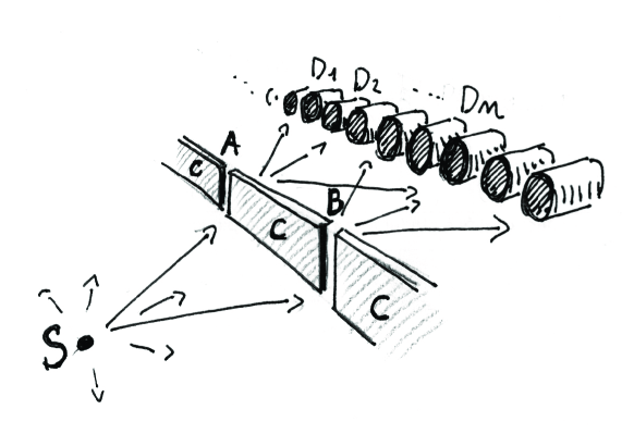
Figure 2: Artistic scheme of the Young’s slit experiment.

To see the implication of the previous formulas and their interpretation, we consider the classical example of the a ‘Young’s slits’-like experiment, extensively considered in the literature (see e.g. Feynman1951 ; BeltramettiCassinelli ; Hughes ).

We consider here the ideal experiment represented in Fig. 2 where a particle is emitted by a source $S$ and detected by a series of detectors $D_{0},\ldots,D_{N}$ after passing through a pair of slits, $A$ and $B$. We assume that the walls of the slits themselves, indicated by $C$, can detect the arrival of particles.

The initial state, i.e. the initial question $Q_{\alpha}^{i}=Q_{\alpha}^{S}$, corresponds to the emission or not of a particle from the source $S$. The detection in proximity of the slits correspond to the questions $Q_{\beta}^{j}$ with $j=\{A,B,C\}$ for the passage through the slits $A$,$B$ or the hitting of the slits walls $C$. The final set of questions corresponds to the detection on the the different detectors on the screen with $Q_{\gamma}^{k}$ with $k=\{D_{0},\ldots,D_{N}\}$. Each set of questions $\{Q_{\beta}^{A},Q_{\beta}^{B},Q_{\beta}^{C}\}$ and $\{Q_{\gamma}^{D_{0}},\ldots,Q_{\gamma}^{D_{N}}\}$ are complete and corresponds to complete bases of Hilbert space $\{\ket{A_{\beta}},\ket{B_{\beta}},\ket{C_{\beta}}\}$ and $\{\ket{D_{0}}_{\gamma},\ldots,\ket{D_{N}}_{\gamma}\}$.

We consider two different cases. In the first one we consider the possibility to distinguish the passage of a particle through $A$ or $B$ (for ex. following the trajectory of the particle if the particle is a ball or another macroscopic object) before being detected on the screen. In the second case, we consider that only the information from the slits wall $C$ is available and we cannot access to the information of the passage through $A$ or $B$. In both case we will study the detection from one particular detector only $D=D_{n}\in\{D_{0},\ldots,D_{N}\}$.

In the first case, because we can distinguish a path between $A$ or $B$, we are considering a detection that correspond to the question structure $(Q_{\gamma}^{D}\ \rotatebox[origin={c}]{90.0}{$\geqslant$}\ Q_{\beta}^{A})\lor(Q_{\gamma}^{D}\ \rotatebox[origin={c}]{90.0}{$\geqslant$}\ Q_{\beta}^{B})$: we want to determine the probability to detect a particle from $D$ passed through $A$ or to detect a particle from $D$ passed throuhg $B$. We are only interested to the detection in $D$ (from here the operator “$\lor^{\prime\prime}$) but we could in principle detect from which slit the particle passed (from here the operator “ $\geqslant$ ”). The probability we are interested is then $p[(Q_{\gamma}^{D}\ \rotatebox[origin={c}]{90.0}{$\geqslant$}\ Q_{\beta}^{A})\lor(Q_{\gamma}^{D}\ \rotatebox[origin={c}]{90.0}{$\geqslant$}\ Q_{\beta}^{B})|Q_{\alpha}^{S}]$ where $Q_{\alpha}^{S}=$ True correspond to a particle emission from the source. Detection of a passage through $A$ or $B$ correspond to mutually exclusive questions $Q_{\beta}^{A}$ and $Q_{\beta}^{B}$ where $Q_{\beta}^{A}\land Q_{\beta}^{B}=\emptyset$. Any combination with these questions, $(Q_{\gamma}^{D}\ \rotatebox[origin={c}]{90.0}{$\geqslant$}\ Q_{\beta}^{A})$ and $(Q_{\gamma}^{D}\ \rotatebox[origin={c}]{90.0}{$\geqslant$}\ Q_{\beta}^{B})$ in our case, is also mutually exclusive as well. Applying Eq. (5c), we have then

$$p[(Q_{\gamma}^{D}\ \rotatebox[origin={c}]{90.0}{$\geqslant$}\ Q_{\beta}^{A})\lor(Q_{\gamma}^{D}\ \rotatebox[origin={c}]{90.0}{$\geqslant$}\ Q_{\beta}^{B})|Q_{\alpha}^{S}]=p[Q_{\gamma}^{D}\ \rotatebox[origin={c}]{90.0}{$\geqslant$}\ Q_{\beta}^{A}|Q_{\alpha}^{S}]+p[Q_{\gamma}^{D}\ \rotatebox[origin={c}]{90.0}{$\geqslant$}\ Q_{\beta}^{B}|Q_{\alpha}^{S}]=\\ =|\braket{D_{\gamma}}{P_{\beta}^{A}}{S_{\alpha}}|^{2}+|\braket{D_{\gamma}}{P_{\beta}^{B}}{S_{\alpha}}|^{2}=\\ =|\braket{D_{\gamma}}{A_{\beta}}\braket{A_{\beta}}{S_{\alpha}}|^{2}+|\braket{D_{\gamma}}{B_{\beta}}\braket{B_{\beta}}{S_{\alpha}}|^{2}.$$ (14)

The final probability is the sum of the individual probabilities (composed each by the square product of different terms) to pass through the slit $A$ and the slit $B$.

In the second case we consider that we cannot distinguish in principle the passage through one specific slit. The non-detection on the walls $C$ after an emission from $S$ corresponds to the certainty of the passage of a particle through $A$ or $B$. Symbolically it means that $\neg Q_{\beta}^{C}\equiv Q_{\beta}^{C^{\bot}}\equiv Q_{\beta}^{A}\lor Q_{\beta}^{B}$. In this case, using Eq. (11), the probability to detect a particle from $D$ is

$$p[Q_{\gamma}^{D}\ \rotatebox[origin={c}]{90.0}{$\geqslant$}\ (Q_{\beta}^{A}\lor Q_{\beta}^{B})|Q_{\alpha}^{S}]=|\braket{D_{\gamma}}{P^{A\lor B}_{\beta}}{S_{\alpha}}|^{2}$$ (15)

with $P^{A\lor B}_{\beta}$ the projector operator corresponding to the positive answer to the question “Is the particle passed through $A$ or $B$?”.

Considering that $\{\ket{j_{\beta}}\}$ basis is orthonormal (formed by mutual exclusive questions), we have that $\braket{j_{\beta}}{k_{\beta}}=0=P^{j}_{\beta}P^{k}_{\beta}$ for $j\neq k$ and then Piron1972

$$P^{A\lor B}_{\beta}=I-P_{\beta}^{A^{\bot}\land B^{\bot}}=I-(I-P_{\beta}^{A})(I-P_{\beta}^{B})=P_{\beta}^{A}+P_{\beta}^{B}.$$ (16)

Using this last equation we have that the final probability is

$$p[Q_{\gamma}^{D}\ \rotatebox[origin={c}]{90.0}{$\geqslant$}\ (Q_{\beta}^{A}\lor Q_{\beta}^{B})|Q_{\alpha}^{S}]=|\braket{D_{\gamma}}{(P_{\beta}^{A}+P_{\beta}^{B})}{S_{\alpha}}|^{2}=\\ =|\braket{D_{\gamma}}{A_{\beta}}\braket{A_{\beta}}{S_{\alpha}}+\braket{D_{\gamma}}{B_{\beta}}\braket{B_{\beta}}{S_{\alpha}}|^{2}.$$ (17)

Differently to the discernible case (Eq. (14)), we have here the square of the sum of two terms with the possibility of interference terms. We have then the well known property of probability calculation of QM without introducing additional postulates or axioms.

In this example we considered only two slits, but it can easily extended to a general case of $N_{s}$ slits. The ensemble of slits correspond to a set of mutually exclusive questions $\{Q_{\beta}^{A},Q_{\beta}^{B},Q_{\beta}^{E},Q_{\beta}^{F},\ldots\}$ with an additional question corresponding to the ensemble of slit walls $Q_{\beta}^{C^{\bot}}\equiv Q_{\beta}^{A}\lor Q_{\beta}^{B}\lor Q_{\beta}^{E}\lor Q_{\beta}^{F}\lor\ldots$ for which Eqs. (14) and (17) can be easily generalized.

4.2 Non-distributivity of the probability argunents

As presented in the previous section, the interference effect on the final probability by one of the detectors $D_{0},D_{1},\ldots,D_{N}$ is directly related to the possibility to distinguish from where the particle passed, i.e. the possibility or not to access to the information relative to the passage through a particular slit. Because of the first RQM postulate, this information can be in fact intrinsically limited. The possibility to distinguish or not the particle path correspond to different conditional probability expressions, Eqs. (14) and (17) respectively. Their equivalence cannot be assumed a priori in the slits experiment example because the distributive property, habitually assumed as valid as in common (classical) cases, is not justified here and can be violated, with in our specific case

$$Q_{\gamma}^{D}\ \rotatebox[origin={c}]{90.0}{$\geqslant$}\ (Q_{\beta}^{A}\lor Q_{\beta}^{B})\neq(Q_{\gamma}^{D}\ \rotatebox[origin={c}]{90.0}{$\geqslant$}\ Q_{\beta}^{A})\lor(Q_{\gamma}^{D}\ \rotatebox[origin={c}]{90.0}{$\geqslant$}\ Q_{\beta}^{B}).$$ (18)

Distributive property is non-valid in question/experiment lattices involving a limited amount of information and it cannot be assumed by default, as presented in a specific example in the Appendix. If distributive property is not given for granted, we have to distinguish the different cases as in the example of Young’s slits experiment. Different cases correspond to different expressions of the probability function $p$, which is uniquely defined by Eqs. (5). What it changes is the proposition combination (question combination) for which we are calculating the probability.

Because of the contradiction with daily experience phenomena where the distributive property is valid, its abandon is, to the opinion of the author, the largest intellectual difficulty in this framework to reconstruct QM formalism from RQM postulates. However the other advantage of RQM formulation is the possibility to transpose the series of questions/measurements to a set of propositions that can be studied then in the context of proposition logic. In the case of the slits experiment, once a particle has been emitted and detected, the sentence “The particle passed through the slit A OR the particle passed through the slit B” is always true. In opposite the sentence “The particle passed through both slits A and B”, equivalent to $Q_{\beta}^{A}\land Q_{\beta}^{B}$ is always False because $Q_{\beta}^{A}$ and $Q_{\beta}^{B}$ are in fact compatible and mutually exclusive with $Q_{\beta}^{A}\land Q_{\beta}^{B}=\emptyset$ ($P^{A}_{\beta}P^{B}_{\beta}=0$). Finally, the sentences “The particle passed through the slit A” and “The particle passed through the slit B” are completely indeterminate if we do not measure where the particle passed through. This is similar to an analog case discussed by Aristotle (reported in Ref.  DallaChiara ) well before the formulation of quantum mechanics. The sentences ‘Tomorrow there will be a sea-battle” and its negation ‘Tomorrow there will not be a sea-battle” have today no definite truth-value (they are indeterminate), but their disjunction “Either tomorrow there will be a sea-battle or tomorrow there will not be a sea-battle” is true. As discussed in Refs. DallaChiara ; Auletta , this structure can be related to the Łukasiewicz three-valued logic approach Bergmann where in addition to the True and False logical values for propositions, an Indeterminate or Unknown third value is considered.

5 Conclusions

In conclusion we demonstrated that from a rigorous definition of the conditional probability for the possible outcomes of different measurements, the Born’s rule and the more general rule with the density operator naturally emerges from the first two postulates of Relational Quantum Mechanics by the use of the Gleason’s theorem. Thus this eliminates the need of introducing a third postulate. In the context of Relational Quantum Mechanics, the approach of the presented work is an alternative to the method adopted by Höhn Hohn2017 ; Hohn2017a ; Hohn2017b . There, the complex field of the reconstructed Hilbert space is univocally determined, but it requires additional postulates and the assumption of the symmetric properties of the probability function $p$. This is not the case in the presented work where symmetric properties of $p$ are derived together with the Born’s rule.

The presence or not of interference terms is demonstrated to be related to the precise formulation of the conditional probability where distributive property cannot be taken for granted. In the specific case of Young’s slits, the violation of distributive property corresponds to a difference between the probability to detect a particle that passed through the pair of slits A and B ($Q_{\gamma}^{D}\ \rotatebox[origin={c}]{90.0}{$\geqslant$}\ (Q_{\beta}^{A}\lor Q_{\beta}^{B})$) and the probability to detect a particle that passed through slit A OR to detect a particle that passed through slit B ($(Q_{\gamma}^{D}\ \rotatebox[origin={c}]{90.0}{$\geqslant$}\ Q_{\beta}^{A})\lor(Q_{\gamma}^{D}\ \rotatebox[origin={c}]{90.0}{$\geqslant$}\ Q_{\beta}^{B})$). Even if the two propositions are apparently equivalent in common language, there is a important difference linked to the possibility or not to determine the particle passage through a particular slit bringing to the disequality $Q_{\gamma}^{D}\ \rotatebox[origin={c}]{90.0}{$\geqslant$}\ Q_{\beta}^{A})\lor(Q_{\gamma}^{D}\ \rotatebox[origin={c}]{90.0}{$\geqslant$}\ Q_{\beta}^{B})\neq Q_{\gamma}^{D}\ \rotatebox[origin={c}]{90.0}{$\geqslant$}\ (Q_{\beta}^{A}\lor Q_{\beta}^{B})$ in the possible probability arguments. The already well known non-validity of distributive property in the logical structure of “yes/no” measurements manifests here once more in the formulation of the probability function $p$.

Appendix A: “Yes/No” measurements and orthomodular lattices

A1 A simple case of distributive and orthocomplemented lattice

To present orthomodular lattices, their properties and their link to a set of “yes/no” experiments, we will consider two simple cases: a classic case relative to the measurement of the size of eggs using two calibers (an example introduced originally by Piron Piron1972 ), and a case of measurement of a spin-1 particle with a Stern-Gerlach apparatus.

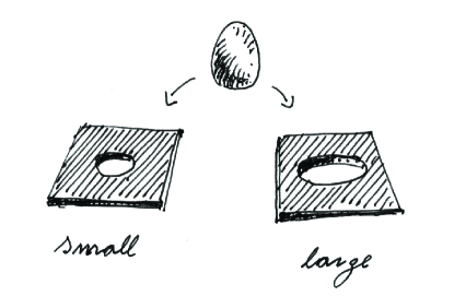
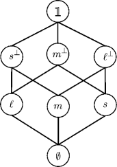
Figure 3: Left: artistic scheme of a egg size measurement with two calibers. Right: graph of the orthocomplemented lattice corresponding to the possible outcomes on the egg size.

In the case of the egg measurement, the questions $\{Q_{\alpha}\}$ associated to these measurements are composed by $Q^{s}=$“is the egg small?”, which positive answer correspond to an egg passing through the small hole with diameter $d_{s}$, and by $Q^{\ell}=$ “is the egg large?” corresponding to an egg not passing through the large hole with diameter $d_{\ell}>d_{s}$ (see Fig. 3 left). From the combination of these two questions we can deduce three sizes: “s” small ($Q^{s}$), “$\ell$” large ($Q^{\ell}$) and “m” medium from the combination $Q^{m}\equiv\lnot Q^{s}\land\lnot Q^{\ell}$.

The different answers (positive or negative) can be interpreted as propositions that can be true or false and are related to each other. As example, if we have a positive answer to the question $Q^{s}$, this corresponds to the proposition “the egg is small” $\equiv s$. If the we have a negative answer (positive to its negation $\lnot Q^{s}$), this corresponds to the proposition “the egg is not small” $\equiv s^{\bot}$, where “$\bot$” indicates complementation (orthogonality) of negative answers with respect to positive answers. In addition to the complementation “$\bot$” we can introduces the operations of conjunction “$\land$” (“AND”), disjunction “$\lor$” (“OR”) between the propositions $s,m,\ell,s^{\bot},m^{\bot},\ell^{\bot}$.

The different answers/propositions and their relation constitute a logical structure of a lattice. As example, a negative answer to the question $Q^{\ell}$, i.e. $\lnot Q^{\ell}$, implies a positive answer to $Q^{m}$ or $Q^{s}$. In this specific example, we have $\ell^{\bot}\implies m\lor s$ (“not large implies medium or small”). This means that for every egg measurement result giving as answers “the egg is medium” or “the egg is small”, we are sure that the proposition “the egg is not large” is true. This order relation (related to the logical implication $\implies$) can be indicated by “$\succeq$”. In the specific example considered, we have that $\ell^{\bot}\succeq m$, $\ell^{\bot}\succeq s$ and $\ell^{\bot}\succeq m\lor s$. This order relation is represented by a graph (Fig. 3 right) by descending lines and where the elements $i\land j$ and $i\lor j$ can be determined joining the two lower or upper lines, respectively, generating from the elements $i$ and $j$.

Due to the question/answer basic structure, each element $i$ of the partially ordered set so defined has a complement $i^{\bot}$ with the properties $i\lor i^{\bot}=\mathbb{1}$ and $i\land i^{\bot}=\emptyset$. $\mathbb{1},\emptyset$ are also part of the set with $\mathbb{1}$ corresponding to all type of eggs and $\emptyset$ to no one. Because of these properties, our partially ordered set is actually a orthocompletemented lattice $\mathcal{L}$. Another important property of the algebra of the lattice defined by this series of measurement is the distributivity (Eq. (1).

Another simple example is the case of a spin-1 particle passing through a Stern-Gerlach apparatus discussed in Sec. 2.2. The complete set of the answers to the questions $\{Q_{V}^{-}\}$ has the same structure as the eggs measurement.

A2 A more complex case; orthomodularity and distributivity

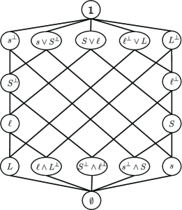
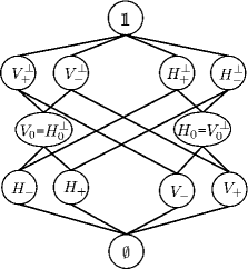
Figure 4: Graphs of the orthocomplemented lattice corresponding to the measurement of egg size with four different calibers (left) and to the measurement with two Stern-Gerlach apparatus, one vertical and one horizontal.

In the classic case of the egg-size determination, a new set of questions $\{Q_{\beta}\}$ corresponds to a new set of calibers with different diameters. We can consider for example, slightly larger holes $d_{S},d_{L}$ with $d_{s}<d_{S}<d_{\ell}<d_{L}$ that correspond to $Q^{S}$ and $Q^{L}$ questions and that generate a new set of possible five measurable sizes. The corresponding lattice is represented in Fig. 4 (left). It is more complex but still distributive. As discussed by Piron Piron1972 ; Piron and Beltrametti and Cassinelli BeltramettiCassinelli , this reflects the fact that the two set of questions (two pairs of calibers) are compatible with each other and that the final measurement output does not depend on the order on which the two pairs of calibers are implemented.

In the case of the spin-1 particle, in addition to a vertically Stern-Gerlach apparatus, we can consider a horizontally oriented one. This new measurement apparatus is related to a new set of questions $\{Q_{H}\}=Q_{H}^{+},Q_{H}^{0},Q_{H}^{-}$ that corresponds to new possible measurement results $\{H_{+},H_{0},H_{-},H^{\bot}_{+},H^{\bot}_{0},H^{\bot}_{-}\}$. When the two sets of measurements are considered together, they form a non-trivial but relatively simple lattice represented in Fig. 4 (right). The perpendicularity of the two apparatus axes determines the fact that a particle giving the measurement result $H_{0}$ in the horizontal apparatus ($V_{0}$) corresponds to a measurement $V_{+}^{\bot}\lor V_{-}^{\bot}$ in the vertical apparatus ($H_{+}^{\bot}\lor H_{-}^{\bot}$ in the horizontal one). The most important characteristic is that the lattice is no more distributive. For example, if we consider the possible outcomes $H_{+},V_{-},V_{-}^{\bot}$, we have that

$$H_{+}\lor(V_{-}\land V_{-}^{\bot})\neq(H_{+}\lor V_{-})\land(H_{+}\lor V_{-}^{\bot}).$$ (19)

In fact the left term is equal to $H_{+}$ and the right term is equal to $V_{-}^{\bot}$.

Additional examples of non-distributive orthomodular lattices can be found in the literature, as the lattice corresponding to the measurement of polarised light Piron1972 or a quantised vector in the real space Hughes .

As discussed by Piron1972 , the distributive property is related to the logical structure of the orthomodular lattice $\mathcal{L}$ corresponding to the ensemble of the measurements. For two elements (“yes/no” measurements) $i,j\in\mathcal{L}$, we have that

$$``i\;\textit{True}^{\prime\prime}\;\text{or}\;``j\;\textit{True}^{\prime\prime}\implies``i\lor j\;\textit{True}^{\prime\prime},$$ (20)

but

$$``i\lor j\;\textit{True}^{\prime\prime}\implies``i\;\textit{True}^{\prime\prime}\;\text{or}\;``j\;\textit{True}^{\prime\prime},$$ (21)

is valid only if the lattice $\mathcal{L}$ is also distributive, which is not the case for measurements reaching the limit of the extractable information, i.e, the quantization aspects Birkhoff1936 ; VonNeumann ; Piron1972 (a simple presentation of this aspect in a Hilbert space can be found in (DallaChiara, , p. 37) and in (Hughes, , p. 190)).

References

- (1) N. Bohr, On the constitution of atoms and molecules, Philos. Mag. 26 (1913), 476–502.
- (2) R. Feynman, The Character of Physical Law, M.I.T. Press, 1967.
- (3) G. Auletta, Foundations and Interpretation of Quantum Mechanics: In the Light of a Critical-historical Analysis of the Problems and of a Synthesis of the Results, World Scientific, 2001.
- (4) L. Hardy, Quantum theory from five reasonable axioms, arXiv preprint quant-ph/0101012.
- (5) R. Clifton, J. Bub, and H. Halvorson, Characterizing quantum theory in terms of information-theoretic constraints, Found. Phys. 33 (2003), 1561–1591.
- (6) A. Grinbaum, Reconstruction of quantum theory, Br. J. Philos. Sci. 58 (2007), 387–408.
- (7) A. Grinbaum, Reconstructing instead of interpreting quantum theory, Philos. Sci. 74 (2007), 761–774.
- (8) B. Dakic and C. Brukner, Quantum theory and beyond: Is entanglement special?, arXiv preprint arXiv:0911.0695.
- (9) P. C. Hohenberg, Colloquium : An introduction to consistent quantum theory, Rev. Mod. Phys. 82 (2010), 2835–2844.
- (10) G. Chiribella, G. M. D’Ariano, and P. Perinotti, Informational derivation of quantum theory, Phys. Rev. A 84 (2011), 012311.
- (11) C. A. Fuchs and R. Schack, Quantum-bayesian coherence, Rev. Mod. Phys. 85 (2013), 1693–1715.
- (12) L. Masanes, M. P. Müller, R. Augusiak, and D. Pérez-García, Existence of an information unit as a postulate of quantum theory, Proc. Natl. Acad. Sci. U.S.A. 110 (2013), 16373–16377.
- (13) H. Barnum, M. P. Müller, and C. Ududec, Higher-order interference and single-system postulates characterizing quantum theory, New J. Phys. 16 (2014), 123029.
- (14) M. Dickson, Reconstruction and reinvention in quantum theory, Found. Phys. 45 (2015), 1330–1340.
- (15) A. Auffèves and P. Grangier, Contexts, systems and modalities: A new ontology for quantum mechanics, Found. Phys. 46 (2016), 121–137.
- (16) R. Friedberg and P. C. Hohenberg, What is quantum mechanics? a minimal formulation, Found. Phys.
- (17) C. Rovelli, Relational quantum mechanics, Int. J. Theor. Phys. 35 (1996), 1637–1678.
- (18) C. Brukner and A. Zeilinger, Operationally invariant information in quantum measurements, Phys. Rev. Lett. 83 (1999), 3354–3357.
- (19) C. Brukner and A. Zeilinger, Young’s experiment and the finiteness of information, Phil. Trans. R. Soc. A 360 (2002), 1061–1069.
- (20) C. A. Fuchs, Quantum mechanics as quantum information (and only a little more), arXiv preprint quant-ph/0205039.
- (21) J. Barrett, Information processing in generalized probabilistic theories, Phys. Rev. A 75 (2007), 032304.
- (22) C. Brukner and A. Zeilinger, Information invariance and quantum probabilities, Found. Phys. 39 (2009), 677–689.
- (23) P. A. Höhn and C. S. P. Wever, Quantum theory from questions, Phys. Rev. A 95 (2017), 012102.
- (24) P. Höhn, Toolbox for reconstructing quantum theory from rules on information acquisition, Quantum 1 (2017), 38.
- (25) P. Höhn, Quantum theory from rules on information acquisition, Entropy 19 (2017), 98.
- (26) J. Yang, Quantum mechanics from relational properties, part I: Formulation, arXiv preprint arXiv:1706.01317.
- (27) J. Yang, Quantum mechanics from relational properties, part II: Measurement, arXiv preprint arXiv:1803.04843.
- (28) J. Yang, Quantum mechanics from relational properties, part III: Path integral implementation, arXiv preprint arXiv:1807.01583.
- (29) M. Smerlak and C. Rovelli, Relational epr, Found. Phys. 37 (2007), 427–445.
- (30) C. Rovelli, ‘space is blue and birds fly through it’, Phil. Trans. R. Soc. A 376.
- (31) D. Poulin, Toy model for a relational formulation of quantum theory, Int. J. Theor. Phys. 45 (2006), 1189–1215.
- (32) M. J. Brown, Relational quantum mechanics and the determinacy problem, Br. J. Philos. Sci. 60 (2009), 679–695.
- (33) B. C. van Fraassen, Rovelli’s world, Found. Phys. 40 (2009), 390–417.
- (34) A. Grinbaum, Information-theoretic princple entails orthomodularity of a lattice, Found. Phys. Lett. 18 (2005), 563–572.
- (35) G. Birkhoff and J. Von Neumann, The logic of quantum mechanics, Ann. Math. 37 (1936), 823–843.
- (36) J. Von Neumann, Mathematical Foundations of Quantum Mechanics, Princeton University Press, 1955.
- (37) E. Beltrametti and G. Cassinelli, The Logic of Quantum Mechanics, Cambridge University Press, 1984.
- (38) R. Hughes, The Structure and Interpretation of Quantum Mechanics, Harvard University Press, 1989.
- (39) M. Dalla Chiara, R. Giuntini, and R. Greechie, Reasoning in Quantum Theory: Sharp and Unsharp Quantum Logics, Springer Netherlands, 2004.
- (40) C. Cohen-Tannoudji, B. Diu, and F. Laloë, Mécanique Quantique, second edition, Hermann, Paris, 1996.
- (41) A. Hájek, Interpretations of probability, in The Stanford Encyclopedia of Philosophy (Winter 2012 Edition), (Edward N. Zalta, ed.), 2012.
- (42) T. Fine, Theories of probability: an examination of foundations, Academic Press, 1973.
- (43) A. Kolmogorov, Foundations of the theory of probability, Chelsea Pub. Co., 1956.
- (44) E. Jaynes and G. Bretthorst, Probability Theory: The Logic of Science, Cambridge University Press, 2003.
- (45) S. Gudder, Quantum Probability, Academic Press, 1988.
- (46) V. Varadarajan, Geometry of Quantum Theory, Springer New York, 2007.
- (47) R. Cox, Algebra of Probable Inference, Johns Hopkins University Press, 1961.
- (48) L. E. Ballentine, Probability theory in quantum mechanics, Am. J. Phys. 54 (1986), 883–889.
- (49) L. E. Ballentine, Propensity, probability, and quantum theory, Found. Phys. 46 (2016), 973–1005.
- (50) A. Auffèves and P. Grangier, Recovering the quantum formalism from physically realist axioms, Sci. Rep. 7 (2017), 43365.
- (51) A. M. Gleason, Measures on the closed subspaces of a hilbert space, J. Math. Mech. 6 (1957), 885–893.
- (52) C. Piron, Survey of general quantum physics, Found. Phys. 2 (1972), 287–314.
- (53) C. Piron, Foundations of quantum physics, Benjamin-Cummings Publishing Company, 1976.
- (54) R. T. Cox, Probability, frequency and reasonable expectation, Am. J. Phys. 14 (1946), 1–13.
- (55) G. D’Agostini, Bayesian Reasoning in Data Analysis: A Critical Introduction, World Scientific, 2003.
- (56) R. P. Feynman, The concept of probability in quantum mechanics, Proceedings of the Second Berkeley Symposium on Mathematical Statistics and Probability, University of California Press, Berkeley, 1951.
- (57) M. Bergmann, An introduction to many-valued and fuzzy logic: semantics, algebras, and derivation systems, Cambridge University Press, 2008.