Properties of the chemostat model with aggregated biomass

Abstract

We revisit the well-known chemostat model, considering that bacteria can be attached together in aggregates or flocs. We distinguish explicitly free and attached compartments in the model and give sufficient conditions for coexistence of these two forms. We then study the case of fast attachment and detachment and shows how it is related to density-dependent growth functions. Finally, we give some insights concerning the cases of multi-specific flocs and different removal rates.

1 Introduction

Attachment and detachment phenomena of bacteria, whether in biofilms on a support [5, 16] or in the form of aggregates or flocs [26] are well known and frequently observed in bacterial growth. Nevertheless, it is only relatively recently that they have been explicitly taken into account in chemostat-based mathematical models. The Freter model [10, 17], proposed in the 1980s as a functional model of the intestine bacterial ecosystem, is one of the very first to explicitly distinguish planktonic biomass from attached biomass. This model considers specific attachment and detachment terms and has been mathematically studied in a spatialized form by introducing advection and diffusion terms [1]. Several works in the biomathematical literature consider extensions to the chemostat model spatialized with (fixed) attachment on a wall by [2, 17, 24]. In general, flocculation models describe the dynamics of the distribution of flocs sizes [26] and their influence on growth dynamics [11], but comparatively there are relatively few studies of simplified models that only distinguish two biomass compartments: planktonic and attached. In [12], it is shown for such models that total biomass growth follows a density-dependent distribution, under the assumption that attachment and detachment velocities are large compared to biological terms. This is in accordance with experimental observations that have showed that the kinetics of processes with attached biomass are better represented by ratio-dependent [13] expressions.

The purpose of the present work is to generalize the existing results concerning these simplified models.

The majority of models of the literature consider explicit attachment and detachment term expressions. We adopt here a more general presentation which does not particularize the specific attachment and detachment kinetics terms and thus namely includes existing models [25, 22, 17]. In every case, the assumptions about faster growth and higher planktonic bacteria removal rate are justified by experimental observations [15]. This allows us to consider reduced models considering the total biomass instead of planktonic and attached ones, which provides extensions of the well-know chemostat model with unusual characteristics.

It should be observed that attachment and detachment velocities can be of a very variable order of magnitude, according to procedures and operating conditions [3], justifying the fact of considering reduced models or not.

2 A general formulation

Under certain growth conditions and in some environments, microbial species may present aggregates of microorganisms or flocs of various sizes (see Figure 1). Microorganisms can also attach themselves to the walls of tanks, pipes, reactors, etc. (or more generally of any chemostat-based device), and thus create biofilms with varied thicknesses. Over time, micro-organisms, parts of flocs or of biofilms, detach and are released in the liquid medium as isolated individuals or small-sized aggregates (see Figure 2). These bacterial assemblages (which can be observed under the microscope) affect the performance of chemostats at the macroscopic level, namely regarding:

• the growth of biomass: bacterial individuals have differentiated access to biotic resource (substrate) depending on their position inside or on the periphery of assemblies. In addition, microorganism secretions of polymers that enable the attachment are generally achieved to the detriment of their growth.

• the disappearance of biomass: flocs and biofilms are most often less likely to be dragged away by the chemostat outflow, comparatively to isolated individuals.

The appearance and evolution mechanisms of these assemblies, which at the same time relate to biology, mechanics and hydrodynamics, are complex, partially understood and difficult to be modeled at a microscopic scale. Our objective is to study how the conventional model of the chemostat can be enriched with considerations reflecting the effects of biomass attachment and detachment at the macroscopic level (in other words, without representing all the refinements that a description would bring at the microscopic level).

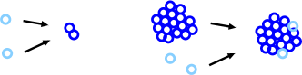
Figure 1: Isolated individuals may aggregate to form a floc, or else attach to an already formed aggregate.

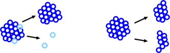
Figure 2: Individuals can detach from an aggregate. An aggregate can be split into smaller aggregates.

We consider that the total biomass of a given species is decomposed into ”planktonic” (or ”free”) biomass made up of non-attached microorganisms (or at least that behave as such; which may still be the case of small assemblies) and ”aggregate” biomass (without accurately taking account of the shape and of the size of assemblies). Thus, we write the concentration $x$ of the total biomass as the sum of concentrations $u$ and $v$ of planktonic and aggregate biomass, respectively:

$$x=u+v\ .$$ (1)

This distinction allows us to take into account different growth and death characteristics according to whether microorganisms are attached or not. We thus denote respectively by $\mu_{u}(\cdot)$, $D_{u}$ and $\mu_{v}(\cdot)$, $D_{v}$ the specific growth and removal rates of planktonic and aggregate compartments. $D_{u}$ and $D_{v}$ are positive numbers and $\mu_{u}(\cdot)$, $\mu_{v}(\cdot)$ are smooth functions that verify $\mu_{u}(0)=\mu_{v}(0)=0$ and positive away from zero. On the other hand, we denote the specific velocities of attachment of planktonic biomass by $\alpha(\cdot)$ and by $\beta(\cdot)$ the ones of detachment of the attached biomass. As a result, we obtain the following chemostat model, where $s$ denotes the substrate concentration:

$$\left\{\begin{array}[]{lll}\displaystyle\frac{ds}{dt}=&\displaystyle D(S_{in}-s)-\mu_{u}(s)u-\mu_{v}(s)v\\[11.38109pt] \displaystyle\frac{du}{dt}=&\mu_{u}(s)u-D_{u}u-\alpha(u,v)u+\beta(v)v\\[11.38109pt] \displaystyle\frac{dv}{dt}=&\mu_{v}(s)v-D_{v}v+\alpha(u,v)u-\beta(v)v\end{array}\right.$$ (2)

The positive parameters $D$ and $S_{in}$ denote the dilution rate and input concentration of the substrate. As usual in chemostat models, we take unit yield coefficients without loss of generality. The simplicity of this representation, which does not account for the richness of forms and possible sizes of aggregates, should be regarded as the considering of an average microorganism behavior within aggregates or biofilms, which differs from that of isolated microorganisms. Since it is difficult to obtain or to justify precise expressions of the attachment and detachment terms for this type of model, our purpose is to understand and qualitatively predict the possible effects of these terms on the dynamics of the system (to this end, we will merely consider simple expressions as possible representatives). It should be noted that the attachment and detachment terms depend on the operating conditions (in particular the flow rate), that we consider here to be fixed.

We first show that the solutions of system (2) stay non-negative and bounded, as in the classical chemostat model.

Lemma 1

The non-negative orthant $\mathbb{R}_{+}^{3}$ is forwardly invariant by the dynamics (2) and any solution in this domain is bounded.

Proof 2.1.

At $s=0$, one has $\dot{s}=DS_{in}>0$. Therefore $s$ stays positive. One has $\frac{d}{dt}(u+v)\geq(\mu_{v}(s)-D_{u})(u+v)$, which shows that $x=u+v$ stay positive. At $u=0$, resp. $v=0$, one has $\frac{d}{dt}u\geq\beta(\cdot)x\geq 0$, resp. $\frac{d}{dt}v\geq\alpha(\cdot)x\geq 0$. Therefore the variables $u$ and $v$ stay non-negative. Finally, on has $\frac{d}{dt}(s+u+v)\leq DS_{in}-D_{v}(s+u+v)$ which shows that the quantity $s+u+v$ is bounded, and a consequence, $s$, $u$ and $v$ also.

Hereafter, we consider the following assumptions, which reflect the considerations discussed in the introduction: The kinetics functions $\mu_{u}(\cdot)$, $\mu_{v}(\cdot)$, $\alpha(\cdot)$, $\beta(\cdot)$ and parameters $D$, $D_{u}$, $D_{v}$ fulfill the following properties.

• The specific growth kinetics $\mu_{u}(\cdot)$ and $\mu_{v}(\cdot)$ are smooth increasing functions, null at zero, that verify:

  $$\mu_{u}(s)>\mu_{v}(s),\quad\forall s>0$$ (3)

• The removal rates of aggregate and planktonic biomass verify:

  $$D\geq D_{u}\geq D_{v}>0$$ (4)

• The function $\alpha$ only depends on concentrations $u$ and $v$ in an increasing manner and such that:

  $$u>0\;\Rightarrow\alpha(u,0)>0$$

  with

  $$\frac{\partial\alpha}{\partial u}(u,v)\geq\frac{\partial\alpha}{\partial v}(u,v),\quad\forall(u,v).$$

• The function $\beta$ depends only on the concentration $v$ in a decreasing manner and such that $v\mapsto\beta(v)v$ is increasing with:

  $$v>0\;\Rightarrow\;\beta(v)>0.$$

Typical instances of functions $\mu_{u}$, $\mu_{v}$ are given by the Monod expression

$$\mu_{\max}\,\frac{s}{K_{s}+s}$$

(with distinct values of the parameters $\mu_{\max}$, $K_{s}$ for planktonic and attached bacteria), that is quite popular in microbiology. Assumption i. expresses the observation that attached bacteria have generally a more difficult acces to substrate. With Assumption ii, we first neglect the mortality of planktonic bacteria, compared to the removal rate $D$, and considered that the substrate is the reactant that is removed most easily because of the the size of its molecules (that is usually much smaller that micro-organisms, justifying the assumption $D_{u}\leq D$). In a similar way, the attachment slows down the effective removal rate of the attached bacteria compared to the planktonic ones (which is represented by the inequality $D_{v}\leq D_{u}$). Typically, it can be considered that the specific attachment velocity $\alpha(u,v)$ can be decomposed into a sum of two terms $\alpha_{u}(u)$ and $\alpha_{v}(v)$ that reflect the two possible types of attachments: on free bacteria or on bacteria already in flocs. Considering that free bacteria mainly attach on the surface of flocs, and that when the size of flocs increases, the ratio surface over volume does not increase as quickly as the volume, it can be expected that the function $\alpha_{v}$ increases more slowly than $\alpha_{u}$, which is then reflected by $\alpha_{u}^{\prime}(u)\geq\alpha_{v}^{\prime}(v)$ for all $(u,v)$, justifying Assumption iii. In general, it is expected that the detachment velocity $v\mapsto\beta(v)v$ increases with the density $v$ of the attached biomass, but when the flocs size increases, the ratio surface over volume increases more slowly than the volume, which results in a decrease of the function $v\mapsto\beta(v)v$, thus justifying Assumption iv.

3 Study of the coexistence between the two forms

We assume that

$$D=D_{u}=D_{v},$$

(the more general case of different removal rates is discussed in Section 5), which allows to consider the variable $z(t)=s(t)+x(t)$, a solution of the differential equation :

$$\frac{dz}{dt}=D(S_{in}-z).$$

whose solutions converge exponentially to $S_{in}$. Therefore, the system (2) has a cascade structure in the $(z,u,v)$ coordinates :

$$\begin{array}[]{l}\displaystyle\frac{dz}{dt}=f_{0}(z)\\[8.53581pt] \displaystyle\frac{du}{dt}=f_{1}(z,u,v),\;\frac{dv}{dt}=f_{2}(z,u,v)\end{array}$$ (5)

and the local stability analysis of its equilibriums is given by the local stability of the equilibriums of the reduced dynamics :

$$\frac{du}{dt}=f_{1}(S_{in},u,v),\;\displaystyle\frac{dv}{dt}=f_{2}(S_{in},u,v)$$ (6)

The global behavior of the solutions of the system (5) is more delicate to be deduced from the global behavior of the reduced system (6) and relies on the theory of asymptotically autonomous systems [21]. However, we recall the well-known result when the reduced system (6)has a unique globally asymptotically stable equilibrium, that states that any bounded solution of (5) converge to the unique equilibrium of (5). We consider in the following the reduced dynamics of (2) for $z=S_{in}$:

$$\left\{\begin{array}[]{lll}\displaystyle\frac{du}{dt}=&\mu_{u}(S_{in}-u-v)u-Du-\alpha(u,v)u+\beta(v)v\\[11.38109pt] \displaystyle\frac{dv}{dt}=&\mu_{v}(S_{in}-u-v)v-Dv+\alpha(u,v)u-\beta(v)v\end{array}\right.$$ (7)

We study the possible positive steady-states $(u^{\star},v^{\star})$ of this system, that is to say, the positive solutions of the system:

$$\left\{\begin{array}[]{l}\displaystyle\mu_{u}(S_{in}-u-v)u-Du-\alpha(u,v)u+\beta(v)v=0\\[11.38109pt] \displaystyle\mu_{v}(S_{in}-u-v)v-Dv+\alpha(u,v)u-\beta(v)v=0\end{array}\right.$$ (8)

It can be immediately noticed that $u^{\star}=0$ implies $\beta(v^{\star})v^{\star}=0$ and $v^{\star}=0$, $\alpha(u^{\star},0)u^{\star}=0$. The assumptions 2.1 that we consider on terms $\alpha(\cdot)$ and $\beta(\cdot)$ then allow us to infer that there is no steady-state where only one of the two forms would be present.

3.1 Coexistence steady-state

Adding equations (8), we obtain $(u^{\star},v^{\star})$ as a solution of the system:

$$\left\{\begin{array}[]{rcrll}(\mu_{u}(s)-D)u&+&(\mu_{v}(s)-D)v&=&0\\ u&+&v&=&S_{in}-s\end{array}\right.$$

Consequently, a coexistence steady-state (if it exists) verifies:

$$u^{\star}=(S_{in}-s^{\star})\frac{D-\mu_{v}(s^{\star})}{\mu_{u}(s^{\star})-\mu_{v}(s^{\star})},\quad v^{\star}=(S_{in}-s^{\star})\frac{\mu_{u}(s^{\star})-D}{\mu_{u}(s^{\star})-\mu_{v}(s^{\star})}$$ (9)

with $s^{\star}=S_{in}-u^{\star}-v^{\star}$. According to hypothesis (3), we obtain the following necessary condition:

$$\mu_{u}(s^{\star})>D>\mu_{v}(s^{\star}).$$

By defining the break-even concentration by $\lambda_{u}$, $\lambda_{v}$ for the dilution rate $D$ (that is that verify $\mu_{u}(\lambda_{u})=\mu_{v}(\lambda_{v})=D$ with $\lambda_{v}>\lambda_{u}$, see [23, 14]), we deduce that a coexistence steady-state must verify:

$$s^{\star}\in(\lambda_{u},\lambda_{v}).$$

Thus, a necessary condition for the existence of a coexistence steady-state is:

$$\lambda_{u}<S_{in}.$$ (10)

At this stage, it is difficult to prove the existence of solutions without specifying attachment and detachment functions $\alpha(\cdot)$ and $\beta(\cdot)$. If we consider that we are only dealing with flocs of small size, as a first approximation it is possible to assume that $\alpha$ is a function of $x=u+v$ (that is, functions $\alpha_{u}$ and $\alpha_{v}$ are identical), which will be chosen as linear (to simplify), and that the function $\beta$ does not depend of $v$:

$$\alpha(u,v)=a(u+v)=ax,\quad\beta(v)=b$$ (11)

where $a$ and $b$ are two positive constants. Thereby, the hypotheses 2.1 are correctly verified.

Proposition 3.1.

For growth functions $\mu_{u}$, $\mu_{v}$ that verify point i) of Assumptions 2.1 and attachment and detachment functions $\alpha(\cdot)$, $\beta(\cdot)$ of the form (11), there exists a unique coexistence steady-state of system (2) if and only if the condition :

$$D<\mu_{u}(S_{in})$$ (12)

is verified.

Proof 3.2.

As mentioned previously, it is enough to show the existence of a positive equilibrium of the reduced dynamics (7). $I$ denotes the interval :

$$I=]\lambda_{u},\lambda_{v}[.$$

To simplify the writing, the following notations are introduced:

$$\varphi_{u}(s)=\mu_{u}(s)-D\quad\mbox{and}\quad\varphi_{v}(s)=\mu_{v}(s)-D.$$

For all $s\in I$, we have $\varphi_{u}(s)>0>\varphi_{v}(s)$. The steady-states $(s^{*},u^{*},v^{*})$ are given by:

$$\left\{\begin{array}[]{lll}0=\varphi_{u}(s^{*})u^{*}-a(u^{*}+v^{*})u^{*}+bv^{*}\\[2.84526pt] 0=\varphi_{v}(s^{*})v^{*}+a(u^{*}+v^{*})u^{*}-bv^{*}.\end{array}\right.$$ (15)

If $u^{*}=0$ then, from the first equation, it can be deduced that $v^{*}=0$. Similarly, if $v^{*}=0$ then, from the second equation it can be deduced that $u^{*}=0$. Consequently, the steady-states are the washout $E_{0}=(S_{in},0,0)$ or a steady-state of the form:

$$E^{*}=(s^{*},u^{*},v^{*})$$

with $u^{*}>0$ , $v^{*}>0$ and $s^{*}=S_{in}-u^{*}-v^{*}$. In order to solve Equations (15), one uses a method similar to the characteristic at steady-state method. This method consists in determining the steady-states of the system formed by the 2nd and 3rd equations of (2), where the variable $s$ is considered to be an input of the system. In other words the aim is to solve the system formed by the first and the second equation of (15), in which $u^{*}$ and $v^{*}$ are the unknowns and $s^{*}$ is considered as being a parameter. It thus yields :

$$u^{*}=U(s^{*}),\qquad v^{*}=V(s^{*}).$$

If $u^{*}$ and $v^{*}$ are replaced by these expressions in the first equation of (2), an equation of the single variable $s^{*}$ is obtained of the form:

$$D(S_{in}-s^{*})=H(s^{*})\quad\mbox{with}\quad H(s^{*})=\mu_{u}(s^{*})U(s^{*})+\mu_{v}(s^{*})V(s^{*})$$

that is solved, see Figure 3, to find a positive solution $s^{*}$ . This solution gives a positive steady-state, provided that $U(s^{*})$ and $V(s^{*})$ be positive. In the following, the functions U, V and H are determined and the conditions are given in order for the solution $s^{*}$ to exist.

Figure 3: Existence of a unique positive steady-state.

By summing the 1st and 2nd equations (15), we obtain:

$$\varphi_{u}(s^{*})u^{*}+\varphi_{v}(s^{*})v^{*}=0.$$ (16)

This equation admits a positive solution if and only if $\varphi_{u}(s^{*})$ and $\varphi_{v}(s^{*})$ are of opposite signs, that is, if and only if $s^{*}\in I$. If this equation admits a solution in this interval then Equation (16) can be written as follows :

$$v^{*}=-\frac{\varphi_{u}(s^{*})}{\varphi_{v}(s^{*})}u^{*}.$$ (17)

By replacing $v^{*}$ by Expression (17) in the first equation of (15), it yields:

$$u^{*}=U(s^{*})\quad\mbox{with}\quad U(s)=\frac{\varphi_{u}(s)(\varphi_{v}(s)-b)}{a[\varphi_{v}(s)-\varphi_{u}(s)]}.$$ (18)

Note that $u^{*}$ defined by (18) is positive because $s^{*}\in I$. By replacing $u^{*}$ by (18) in (17), we get:

$$v^{*}=V(s^{*})\quad\mbox{with}\quad V(s)=-\frac{\varphi_{u}^{2}(s)(\varphi_{v}(s)-b)}{a[\varphi_{v}(s)-\varphi_{u}(s)]\varphi_{v}(s)}.$$ (19)

Substituting the expressions of $U(s^{*})$ and $V(s^{*})$ given by (18) and (19) in the expression of $H(s^{*})$ yields a characterization of $s^{*}$:

$$D(S_{in}-s^{*})=H(s^{*})\quad\mbox{with}\quad H(s)=D\frac{\varphi_{u}(s)(\varphi_{v}(s)-b)}{a\varphi_{v}(s)}.$$ (20)

Note that for all $s\in I$ , $U(s)>0$, $V(s)>0$ and $H(s)>0$ and that :

$$\lim_{s\to\lambda_{u}}H(s)=0,\quad\lim_{s\to\lambda_{v}}H(s)=+\infty.$$

In addition, function $H$ is strictly increasing on $I$. Indeed, we have:

$$H^{\prime}(s)=\frac{D}{a}\frac{\varphi_{v}(s)(\varphi_{v}(s)-b)\varphi_{u}^{\prime}(s)+b\varphi_{u}(s)\varphi_{v}^{\prime}(s)}{\varphi_{v}^{2}(s)}>0.$$

Consequently, Equation (20) admits a unique solution $s^{*}\in I=]\lambda_{u},\lambda_{v}[$ if and only if $S_{in}>\lambda_{u}$, which is equivalent to $\mu_{u}(S_{in})>D$.

3.2 Study of stability

Under the conditions of stability and global attractiveness of the washout steady-state of the chemostat model in which only the planktonic biomass would be considered (see [23, 14]):

$$D\geq\mu_{u}(S_{in})$$ (21)

one can easily check that the washout $(S_{in},0,0)$ is also the only steady-state of the system (2), stable and globally attractive. As a matter of fact, by considering the reduced model (7), under this assumption we have:

$$x\in]0,S_{in}]\;\Rightarrow\;\frac{dx}{dt}=(\mu_{u}(S_{in}-x)-D)u+(\mu_{v}(S_{in}-x)-D)v<0$$

which demonstrates that $x(\cdot)$ asymptotically converges towards $0$ for any initial condition. As any solution of system (2) is bounded, we deduce that it converges to the washout equilibrium. According to the study conducted in Section 3.1, a positive steady-state exists as soon as the condition (12) is verified and is unique. By particularizing the attachment and detachment functions as we did in Section 3.1, the following stability result is obtained (the case in which $D_{u}$ and $D_{v}$ are different from $D$ is addressed in [8]).

Proposition 3.3.

Under the assumptions of Proposition 3.1 the coexistence steady-state is a locally exponentially stable of system (2).

Proof 3.4.

As mentioned previously, it is enough to study the local stability for the reduced dynamics (7). The Jacobian matrix of (7) for the steady-state $(u^{*},v^{*})$, which corresponds to the positive equilibrium $E^{*}=(s^{*},u^{*},v^{*})$ of (2), is equal to:

$$J^{*}=\left[\begin{array}[]{ll}-u^{*}\varphi_{u}^{\prime}(s^{*})+\varphi_{u}(s^{*})-a(2u^{*}+v^{*})&-u^{*}\varphi_{u}^{\prime}(s^{*})-au^{*}+b\\[5.69054pt] -v^{*}\varphi_{v}^{\prime}(s^{*})+a(2u^{*}+v^{*})&-v^{*}\varphi_{v}^{\prime}(s^{*})+\varphi_{v}(s^{*})+au^{*}-b\end{array}\right]$$

The trace of this matrix is equal to:

$${\rm Tr}J^{*}=-u^{*}\varphi_{u}^{\prime}(s^{*})-v^{*}\varphi_{v}^{\prime}(s^{*})+\varphi_{u}(s^{*})-a(u^{*}+v^{*})+\varphi_{v}(s^{*})-b$$

Note that based on Equations (15), it can be deduced that:

$$\varphi_{u}(s^{*})-a(u^{*}+v^{*})=-b\frac{v^{*}}{u^{*}}<0,\qquad\varphi_{v}(s^{*})-b=-a\frac{(u^{*}+v^{*})u^{*}}{v^{*}}<0$$ (22)

Further, as $\varphi_{u}^{\prime}(s^{*})>0$ and $\varphi_{v}^{\prime}(s^{*})>0$, it can be deduced that ${\rm Tr}J^{*}<0$. The determinant of this matrix is equal to:

$${\rm Det}J^{*}=Au^{*}\varphi_{u}^{\prime}(s^{*})+Bv^{*}\varphi_{v}^{\prime}(s^{*})+C$$

with:

$$A=a(u^{*}+v^{*})+b-\varphi_{v}(s^{*}),\quad B=a(u^{*}+v^{*})+b-\varphi_{u}(s^{*}),$$

and:

$$C=\varphi_{u}(s^{*})\varphi_{v}(s^{*})+\varphi_{u}(s^{*})(au^{*}-b)-\varphi_{v}(s^{*})a(2u^{*}+v^{*})$$

By using Expressions (22), it yields that:

$$A=a\frac{(u^{*}+v^{*})^{2}}{v^{*}}>0,\quad B=b\frac{u^{*}+v^{*}}{u^{*}}>0$$

Moreover, we have:

$$C=\varphi_{u}(s^{*})\left(\varphi_{v}(s^{*})-b\right)+a\left(u^{*}\varphi_{u}(s^{*})-v^{*}\varphi_{v}(s^{*})\right)-2au^{*}\varphi_{v}(s^{*})$$

Utilizing (16), we get:

$$C=\varphi_{u}(s^{*})\left(\varphi_{v}(s^{*})-b\right)+2au^{*}\varphi_{u}(s^{*})-2au^{*}\varphi_{v}(s^{*})$$

Utilizing (22), we have:

$$au^{*}\left(\varphi_{u}(s^{*})-\varphi_{v}(s^{*})\right)=-\varphi_{u}(s^{*})\left(\varphi_{v}(s^{*})-b\right)$$

Consequently:

$$C=-\varphi_{u}(s^{*})\left(\varphi_{v}(s^{*})-b\right)>0$$

Thereof, it can be deduced that ${\rm Det}J^{*}>0$, and as a consequence, the real parts of the eigenvalues of $J^{*}$ are strictly negative.

4 The case of fast attachments/detachments

Depending on species and on hydrodynamic conditions, attachment and detachment velocities may prove to be large compared to growth kinetics and to dilution rate. In this case, it is possible to consider that the attachment and detachment terms, $\alpha(\cdot)$ and $\beta(\cdot)$ respectively, can be rewritten in the form:

$$\frac{\alpha(\cdot)}{\varepsilon},\quad\frac{\beta(\cdot)}{\varepsilon}$$

where $\varepsilon$ is a positive number supposed to be small, and functions $\alpha(\cdot)$, $\beta(\cdot)$ verify the same assumptions 2.1. Thus, the model (2) is written as:

$$\left\{\begin{array}[]{lll}\displaystyle\frac{ds}{dt}&=&\displaystyle D(S_{in}-s)-\mu_{u}(s)u-\mu_{v}(s)v\\[11.38109pt] \displaystyle\frac{du}{dt}&=&\displaystyle\mu_{u}(s)u-Du-\frac{1}{\epsilon}\left(\alpha(u,v)u-\beta(v)v\right)\\[11.38109pt] \displaystyle\frac{dv}{dt}&=&\displaystyle\mu_{v}(s)v-Dv+\frac{1}{\epsilon}\left(\alpha(u,v)u-\beta(v)v\right)\end{array}\right.$$ (23)

It is convenient to write this dynamic by replacing the variables $u$ and $v$ by $x=u+v$ and $p=u/x$

$$\left\{\begin{array}[]{lll}\displaystyle\frac{ds}{dt}&=&\displaystyle D(S_{in}-s)-\bar{\mu}(s,p)x\\[11.38109pt] \displaystyle\frac{dx}{dt}&=&\displaystyle\bar{\mu}(s,p)x-Dx\\[11.38109pt] \displaystyle\frac{dp}{dt}&=&\displaystyle\left(\mu_{u}(s)-\mu_{v}(s)\right)p(1-p)-\frac{1}{\epsilon}\left(\alpha(px,(1-p)x)p-\beta((1-p)x)(1-p)\right)\end{array}\right.$$ (24)

by defining:

$$\bar{\mu}(s,p):=p\,\mu_{u}(s)+(1-p)\,\mu_{v}(s).$$

Observe that this dynamic system is of the form:

$$\left\{\begin{array}[]{lll}\displaystyle\frac{ds}{dt}&=&\displaystyle f_{s}(s,x,p)\\[11.38109pt] \displaystyle\frac{dx}{dt}&=&\displaystyle f_{x}(s,x,p)\\[11.38109pt] \displaystyle\frac{dp}{dt}&=&\displaystyle\frac{1}{\epsilon}\left[\epsilon f_{p}(s,p)+g(x,p)\right]\end{array}\right.$$

where we posit:

$$g(x,p):=-\alpha(px,(1-p)x)p+\beta((1-p)x)(1-p).$$

When $\epsilon$ is small and the terms $f_{s}(s,x,p)$, $f_{x}(s,x,p)$ and $\epsilon f_{p}(s,p)+g(x,p)$ are of the same order of magnitude, the velocity $\frac{dp}{dt}$ is then very large compared to velocities $\frac{ds}{dt}$, $\frac{dx}{dt}$. Variables $s$ and $x$ can then be considered as almost constant and the approximation of the dynamics of variable $p$ as ”fast”:

$$\frac{dp}{dt}=\frac{1}{\epsilon}g(x,p)$$ (25)

where $s$ is considered as a constant parameter (the term $\epsilon f_{p}(s,p)$ being negligible with regard to $g(x,p)$). If for any $x$, the differential equation (25) admits a unique steady-state $\bar{p}(x)$, then this expression can be carried to the system (24) to obtain the ”slow” approximation of the dynamics of the variables $s$ and $x$:

$$\left\{\begin{array}[]{lll}\displaystyle\frac{ds}{dt}&=&\displaystyle D(S_{in}-s)-\mu(s,x)x\\[11.38109pt] \displaystyle\frac{dx}{dt}&=&\displaystyle\mu(s,x)x-Dx\end{array}\right.$$ (26)

by defining:

$$\mu(s,x)=\bar{\mu}(s,\bar{p}(x)).$$

This reduction technique (which consists in replacing $\epsilon$ by $0$) is well known in physics under the name of quasi-steady state approximation method. At the mathematical level, the rigorous proof of the convergence of the solutions of the system (24) towards those of the reduced system (26) makes use of the theory of singular perturbations (see for instance [18]). When the slow manifold is globally attractive, that is when $\bar{p}(x)$ is a globally asymptotically stable of the dynamics $dp/d\tau=g(x,p)$ for any fixed $x>0$ (where $\tau=t/\epsilon$ is the “fast” time), then Tikhonov’s Theorem applies. Recall that this Theorem asserts that for any initial condition of (24) with $x(0)>0$ and any time interval $[0,T]$ with $T>0$, the solution $s(\cdot)$, $x(\cdot)$ of (24) converge uniformly on $[0,T]$ to the solution of (26). Furthermore, when the solution of the reduced dynamics (26) converges to an asymptotically stable equilibrium, then one can take $T=+\infty$ (see for instance [20]). The Proposition below shows that the existence and the global asymptotic stability of the slow manifold, under Assumptions 2.1.

Proposition 4.1.

Under Assumptions 2.1, there exists a unique function $\bar{p}:\mathbb{R}_{+}\mapsto[0,1]$ $C^{1}$, strictly decreasing, such that $g(x,\bar{p}(x))=0$ for all $x>0$. In addition, $\bar{p}(x)$ is the unique globally asymptotically stable steady-state of the scalar equation (25), for all $x>0$.

Proof 4.2.

For any $x>0$, we have $g(x,0)=\beta(x)>0$ and $g(x,1)=-\alpha(x,0)<0$ (following Assumptions 2.1). According to the intermediate value theorem, there therefore exists $\bar{p}(x)\in]0,1[$ such that $g(x,\bar{p}(x))=0$. Let us determine the partial derivatives of the function $g$:

$$\begin{array}[]{lll}\displaystyle\frac{\partial g}{\partial x}&=&\displaystyle-\left[\left(\frac{\partial\alpha}{\partial u}(u,v)p+\frac{\partial\alpha}{\partial v}(u,v)(1-p)\right)p-\beta^{\prime}(v)(1-p)^{2}\right]_{u=px,v=(1-p)x}\\[14.22636pt] \displaystyle\frac{\partial g}{\partial p}&=&\displaystyle-\left[\left(\frac{\partial\alpha}{\partial u}(u,v)-\frac{\partial\alpha}{\partial v}(u,v)\right)u+\alpha(u,v)+\frac{1}{u+v}\frac{d}{dv}(\beta(v)v)\right]_{u=px,v=(1-p)x}\end{array}$$

For $x>0$, Assumptions 2.1 guarantee $\frac{\partial g}{\partial x}<0$ and $\frac{\partial g}{\partial p}<0$. Thus, the function $p\mapsto g(x,p)$ is strictly decreasing, guaranteeing the uniqueness of the solution $\bar{p}(x)$ of $g(x,p)=0$. According to the implicit function theorem, the function $\bar{p}$ is also differentiable for any $x>0$ and its derivative is written as:

$$\bar{p}^{\prime}(x)=-\frac{\displaystyle\frac{\partial g}{\partial x}(x,\bar{p}(x))}{\displaystyle\frac{\partial g}{\partial p}(x,\bar{p}(x))}<0.$$

The function $\bar{p}$ is thus $C^{1}$ on $\mathbb{R}_{+}\setminus\{0\}$ and strictly decreasing. Thereby, for all fixed $x>0$, $\bar{p}(x)$ is the unique steady-state of the differential equation (25), and since $\frac{\partial g}{\partial p}<0$ for every $(x,p)$, it can be thereof deduced that the steady-state $\bar{p}(x)$ is globally asymptotically stable for the scalar dynamics (25).

For instance, for functions considered in (11), we get:

$$\bar{p}(x)=\frac{1}{\displaystyle 1+\frac{a}{b}x}.$$ (27)

Figure 4 presents simulations with functions (11) and compares the solutions (in plain line) of the original system (24) with the ones (in dashed line) of the reduced dynamics (26). It shows that the slow-fast approximation is good even for value of $\epsilon$ that are not so small.

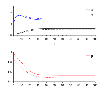
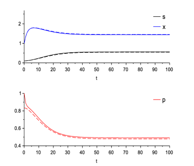
Figure 4: Simulations for $\mu_{u}(s)=\frac{s}{1+s}$, $\mu_{v}(s)=\frac{0.7s}{1+s}$, $S_{in}=2$, $D=0.5$, $a=1$, $b=0.5$ with $\epsilon=2$ (left) and $\epsilon=0.5$ (right)

Remark 4.3.

Thanks to Assumptions 2.1, it yields that:

$$\frac{\partial\mu}{\partial x}(s,x)=\frac{\partial\bar{\mu}}{\partial p}(s,p)|_{p=\bar{p}(x)}.\bar{p}^{\prime}(x)=(\mu_{u}(s)-\mu_{v}(s)).\bar{p}^{\prime}(x)<0$$

and thus the model (26) for the total biomass $x$ has a density-dependent growth, decreasing with respect $x$.

4.1 Consideration of several species

When several species are in competition, we can similarly decompose the biomass of each species $i$ into planktonic biomass $u_{i}$ and attached biomass $v_{i}$ (without differentiating the composition of flocs which can mix individuals from different species):

$$\left\{\begin{array}[]{lll}\displaystyle\frac{ds}{dt}=&\displaystyle D(S_{in}-s)-\sum_{j=1}^{n}\mu_{u_{j}}(s)u_{j}-\sum_{j=1}^{n}\mu_{v_{j}}(s)v_{j}\\[11.38109pt] \displaystyle\frac{du_{i}}{dt}=&\mu_{u_{i}}(s)u_{i}-Du_{i}-\alpha_{i}(u_{1},\cdots,u_{n},v_{1},\cdots,v_{n})u_{i}+\beta(v_{1},\cdots,v_{n})v_{i}\\ &&\hfill(i=1\cdots n)\\ \displaystyle\frac{dv_{i}}{dt}=&\mu_{v_{i}}(s)v_{i}-Dv_{i}+\alpha_{i}(u_{1},\cdots,u_{n},v_{1},\cdots,v_{n})u_{i}-\beta(v_{1},\cdots,v_{n})v_{i}\end{array}\right.$$

The specific attachment functions $\alpha_{i}$ then depend (a priori) on all others quantities $u_{j}$, $v_{j}$ since a free individual of species $i$ can attach to free biomass or biomass with any species attached. Analogously, the specific detachment functions $\beta_{i}$ depend a priori on all quantities $v_{j}$ of biomass attached where an individual $i$ could have attached. To simplify, it will be possible, for example, to assume that the $\alpha_{i}$ are functions of the total planktonic and attached biomass $u=\sum_{j}u_{j}$ and $v=\sum_{v}v_{j}$, and the $\beta_{i}$ functions of $v$ only, with the same Assumptions (2.1). The combinatorics of the possible specific cases makes the mathematical study much more complicated, but when the attachment and detachment velocities can be considered to be fast, the quasi-steady state approximation makes it possible to write a dynamic system for biomass $x_{i}=u_{i}+v_{i}$ by expressing the terms $u_{i}$ and $v_{i}$ according to all the $x_{j}$ on the ”slow” manifold defined by the system of equations:

$$\alpha_{i}(u_{1},\cdots,u_{n},v_{1},\cdots,v_{n})u_{i}-\beta_{i}(v_{1},\cdots,v_{n})v_{i}=0\qquad i=1\cdots n.$$

For example, by considering simple functions like we did in (11):

$$\alpha_{i}(x_{1},\cdots,x_{n})=\sum_{j=1}^{n}a_{ij}x_{j},\quad\beta_{i}=b_{i}$$

where parameters $a_{ij}$ reflect how easily an individual of species $i$ attaches to an individual of species $j$, the following expressions are obtained for the proportions $q_{i}=u_{i}/x_{i}$ on the slow manifold, which is uniquely defined by

$$\bar{q}_{i}(x_{1},\cdots,x_{n})=\frac{1}{\displaystyle 1+\frac{1}{b_{i}}\sum_{j=1}^{n}a_{ij}x_{j}}$$

as in Section 4 (under the assumption of fast attachments and detachments), and the reduced system is then written as:

$$\left\{\begin{array}[]{lll}\displaystyle\frac{ds}{dt}&=&\displaystyle D(S_{in}-s)-\sum_{j=1}^{n}\mu_{j}(s,x_{1},\cdots,x_{n})x_{j}\\[11.38109pt] \displaystyle\frac{dx_{i}}{dt}&=&\displaystyle\mu_{i}\left(s,x_{1},\cdots,x_{n}\right)x_{i}-Dx_{i}\qquad(i=1\cdots n)\end{array}\right.$$

by setting:

$$\mu_{i}(s,x)=\bar{q}_{i}(x_{1},\cdots,x_{n})\mu_{u_{i}}(s)+(1-\bar{q}_{i}(x_{1},\cdots,x_{n}))\mu_{v_{i}}(s)$$

The dynamics of the fast variables $q_{i}$ is given by the system

$$\frac{dq_{i}}{d\tau}=-\alpha_{i}(x)q_{i}+b_{i}(1-q_{i})\qquad(i=1\cdots n)$$

(where $\tau=t/\epsilon)$ for which $(\bar{q}_{1},\cdots,\bar{q}_{n})$ is clearly the unique globally asymptotically stable equilibrium, for any fixed $(x_{1},\cdots,x_{n})$. Therefore Thikonov’s Theorem applies. Notice that $\mu_{i}$ are density-dependent growth functions, decreasing with respect to the $x_{i}$. This then exactly corresponds to the context of density-dependent competition model, which shows that a coexistence between species is possible [19, 6]. It is thus concluded that a mechanism of (fast) attachment and detachment of biomass is a possible (theoretical) explanation for the maintaining of biodiversity in a chemostat.

5 Consideration of distinct removal rates

In this Section, we consider that the removal rates of planktonic and attached bacteria are distinct, and accordingly to Assumptions (2.1) one has $D_{v}<D_{u}\leq D$. This Section follows part of the work [7, 8]. The reduction technique we use in Section 4 gives the following reduced model:

$$\left\{\begin{array}[]{lll}\displaystyle\frac{ds}{dt}&=&\displaystyle D(S_{in}-s)-\mu(s,x)x\\[11.38109pt] \displaystyle\frac{dx}{dt}&=&\displaystyle\mu(s,x)x-d(x)x\end{array}\right.$$ (28)

where we posit:

$$d(x)=\bar{p}(x)D_{u}+(1-\bar{p}(x))D_{v}.$$

Notice that the dynamics of the fast variable $p$ is given by equation (25), exactly as in Section 4. Therefore, Proposition 4.1 applies. Let us underline that having a density dependent removal rate in the chemostat model has not being considered (and justified) before in the literature.

As in Section 3.1, we consider break-even concentrations $\lambda_{u}$, $\lambda_{v}$ associated to functions $\mu_{u}$ and $\mu_{v}$ but here for the distinct removal rates $D_{u}$, $D_{v}$ (which are numbers that verify $\mu_{u}(\lambda_{u})=D_{u}$ and $\mu_{v}(\lambda_{v})=D_{v}$). Differently to the case of identical removal rates, for which Assumptions 2.1 implies the inequality $\lambda_{u}<\lambda_{v}$, this later inequality is no longer necessarily satisfied, as depicted on Figure 5.

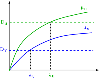
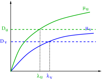
Figure 5: One can have $\lambda_{u}>\lambda_{v}$ (left) as well as $\lambda_{u}<\lambda_{v}$ (right).

The model (28) admits clearly the washout $(S_{in},0)$ as an equilibrium, and let us study the possibility for the system to have another steady state. A positive equilibrium $(s^{\star},x^{\star})$ of dynamics (28) has to fulfill

$$s^{\star}=\gamma(x^{\star}):=S_{in}-\frac{x^{\star}d(x^{\star})}{D}$$ (29)

and

$$\mu(s^{\star},x^{\star})=d(x^{\star})$$ (30)

Notice that when $s<\min(\lambda_{u},\lambda_{v})$, resp. $s>\max(\lambda_{u},\lambda_{v})$, one has $\mu(s,x)<d(x)$, resp. $\mu(s,x)>d(x)$, for any $x$. Therefore, one has

$$s^{\star}\in[\min(\lambda_{u},\lambda_{v}),\max(\lambda_{u},\lambda_{v})].$$

Since the functions $\mu_{u}$ and $\mu_{v}$ are increasing, the map $s\mapsto\mu(s,x)$ is increasing for any $x$ and by the Implicit Function Theorem, we deduce the existence of an unique solution of (30) as $s^{\star}=\phi(x^{\star})$. Therefore, a positive equilibrium (if it exists) has to fulfill

$$\Gamma(x^{\star}):=\gamma(x^{\star})-\phi(x^{\star})=0.$$

Notice that one has $\Gamma(0)=S_{in}-\lambda_{u}$ and $\Gamma(+\infty)=-\infty$. Therefore, the existence of a positive equilibrium is guaranteed when $\lambda_{u}<S_{in}$. Notice that this last condition is exactly the one that guarantees the existence of a positive equilibrium for the chemostat model without attachment:

$$\left\{\begin{array}[]{lll}\displaystyle\frac{ds}{dt}&=&\displaystyle D(S_{in}-s)-\mu_{u}(s)u\\[11.38109pt] \displaystyle\frac{du}{dt}&=&\displaystyle\mu_{u}(s)u-D_{u}u\end{array}\right.$$

We examine now the possibilities of having more than one positive equilibrium. The function $\gamma$ is such that $\gamma(0)=S_{in}$ and $\gamma(+\infty)=-\infty$. So, it has to decrease somewhere on the interval $[0,+\infty)$. From the Implicit Function Theorem, we can write

$$\phi^{\prime}(x)=\frac{d^{\prime}(x)-\frac{\partial\mu}{\partial x}(\phi(x),x)}{\frac{\partial\mu}{\partial s}(\phi(x),x)}=\frac{\bar{p}^{\prime}(x)}{\frac{\partial\mu}{\partial s}(\phi(x),x)}\left(D_{u}-D_{v}-\mu_{u}(\phi(x))+\mu_{v}(\phi(x))\right)$$

When $\lambda_{u}<\lambda_{v}$, one has $\mu_{u}(s)\geq D_{u}$ and $\mu_{v}(s)<D_{v}$ for any $s\in[\lambda_{u},\lambda_{v})$. As $\bar{p}^{\prime}(x)<0$ (see Proposition 4.1) and $\frac{\partial\mu}{\partial s}(\phi(x),x)>0$, we deduce $\phi^{\prime}(x)>0$ for any $x$ such that $\phi(x)\in[\lambda_{u},\lambda_{v})$. At the opposite, when $\lambda_{u}>\lambda_{v}$, one has $\phi^{\prime}(x)<0$ for any $x$ such that $\phi(x)\in[\lambda_{v},\lambda_{u})$. This leaves open the possibility of having the functions $\gamma$ and $\phi$ simultaneously decreasing with more than one intersection of their graphs (and then having the function $\Gamma$ non-monotonic with alternate signs of $\Gamma^{\prime}(x^{\star})$ at the solutions $x^{\star}$). At a positive equilibrium $E^{*}=(s^{*},x^{*})$, the Jacobian matrix is:

$$J(E^{*})=\left[\begin{array}[]{cc}\displaystyle-D-x^{*}\frac{\partial\mu}{\partial s}(s^{*},x^{*})&\displaystyle-x^{*}\frac{\partial\mu}{\partial x}(s^{*},x^{*})-d(x^{*})\\[11.38109pt] \displaystyle x^{*}\frac{\partial\mu}{\partial s}(s^{*},x^{*})&\displaystyle x^{*}\frac{\partial\mu}{\partial x}(s^{*},x^{*})-x^{*}d^{\prime}(x^{*})\end{array}\right]$$

with determinant:

$$detJ(E^{*})=Dx^{*}\left(d^{\prime}(x^{*})-\frac{\partial\mu}{\partial x}(s^{*},x^{*})\right)+x^{*}\frac{\partial\mu}{\partial s}(s^{*},x^{*})\frac{d}{dx}[xd(x)](x^{*}).$$

One can easily check that it can be also written as

$$detJ(E^{*})=-Dx^{*}\frac{\partial\mu}{\partial x}(s^{*},x^{*})\Gamma^{\prime}(x^{*})$$

which shows an alternation of stability of the equilibriums $E^{*}$ depending on the sign of $\Gamma^{\prime}(x^{*})$. We illustrate the possibility of having multiple-stability in the case $\lambda_{v}<\lambda_{u}<S_{in}$ with the functions $\alpha$, $\beta$ given in (11), that provide the simple expression (27) of the function $\bar{p}(\cdot)$, and Monod expressions for functions $\mu_{u}$, $\mu_{v}$. Even in this simple case, the expression of the function $\Gamma$ is too complicated to conduct an analytic study. Figure 6 presents the phase portrait of the reduced dynamics (28) and shows its bi-stability for the numerical values of the parameters that have been chosen.

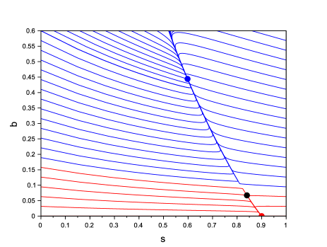
Figure 6: Example of bi-stability with $\mu_{u}(s)=\frac{2s}{1+s}$, $\mu_{v}(s)=\frac{1.5s}{0.8+s}$, $D_{u}=1$, $D_{v}=0.5$, $S_{in}=0.9$, $D=1$, $a/b=4$.

In the reference [7], it is shown that under the additional assumption that the map $x^{*}\mapsto x^{*}\bar{p}(x^{*})$ is increasing, the multiplicity can indeed occur only when $\lambda_{u}>\lambda_{v}$, and that generically each equilibrium is necessarily either a stable node or a saddle point. Therefore, Tikhonov’s Theorem, that has been recalled in Section 4, allows to claim that for any initial condition of the system (2) such that $(s_{0},x_{0})$ does not belong to the stable manifold of a saddle equilibrium of the reduced dynamics (28), the solution $s(\cdot)$, $x(\cdot)$ converges to the solution of the reduced dynamics on the $[0,+\infty)$ time interval, that is for almost any initial condition.

Finally, this shows that multiple stability can occur in the chemostat model with attachment and distinct removal rates, even though the growth functions are monotonically increasing. This fact is quite remarkable comparing to the classical chemostat model (i.e. without attachment) for which a multiple stability is possible only for non-monotonic growth functions (see for instance [14]). Nevertheless, the analysis of all the generic behaviors of the solutions of the model with several species (and different removal rates) remains today an open problem. Dynamics in dimension higher than two potentially reserve a richness of possible behaviors. In particular, the possibility of having unstable nodes leave open the possibilities of having limit cycles, as illustrated in [9].

6 Conclusion

In this work we have proposed a generic framework of chemostat models with free and attached biomass compartments. Under general assumptions, we have shown that a coexistence of the two forms is possible and leads to a unique positive equilibrium which is moreover globally asymptotically stable. When the assumptions about fast attachment and detachment are justified, we have also shown that reduced models with the total biomass instead of planktonic and attached ones provide natural extensions of the classical chemostat model with a density-dependent growth function, such as in the Contois model [4]. This allows coexistence of multiple species when each of them can be present in the two forms: planktonic and attached (with same or different species). We have also shown that the consideration of different removal rates for the free and attached biomass could lead to some non-intuitive behaviors, such as multiple stability, that is today widely not well understood in presence of several species.

This work has been initiated in the “DISCO” project funded by the French National Research Agency (ANR) in the SYSCOMM program. The author warmly thanks T. Sari, C. Lobry, J. Harmand and R. Fekih-Salem, whose PhD work having inspired the present paper.

References

- [1] M. Ballyk, D. Jones, and H. Smith. The Biofilm Model of Freter: a review, pages 265–302. Ed. Magal, P. and Ruan, S., Springer-Verlag, 2008.
- [2] M. Ballyk and H. Smith. A model of microbial growth in a plug flow reactor with wall attachment. Mathematical Biosciences, 158:95–126, 1999.
- [3] A. Berlin and V. Kislenko. Kinetic models of suspension flocculation by polymers. Colloids Surf. A: Physicochem. Eng. Asp., 104:67–72, 1995.
- [4] D. Contois. Kinetics of bacterial growth: relationship between population density and specific growth rate of continuous cultures. J. Gen Microbiol., 21:40–50, 1959.
- [5] J. Costeron. Overview of microbial biofilms. J. Indust. Microbiol., 15:l37–140, 1995.
- [6] P. De Leenheer, D. Angeli, and E. Sontag. Crowding effects promote coexistence in the chemostat. Journal of Mathematical Analysis and Applications, 319(1):48–60, 2006.
- [7] R. Fekih-Salem. Modéles mathématiques pour la compétition et la coexistence des espéces microbiennes dans un chémostat. PhD thesis, University of Montpellier II and University of Tunis el Manar., 2013. https://tel.archives-ouvertes.fr/tel-01018600.
- [8] R. Fekih-Salem, J. Harmand, C. Lobry, A. Rapaport, and T. Sari. Extensions of the chemostat model with flocculation. J. Math. Anal. Appl., 397:292–306, 2013.
- [9] R. Fekih-Salem, A. Rapaport, and T. Sari. Emergence of coexistence and limit cycles in the chemostat model with flocculation for a general class of functional responses. Applied Mathematical Modelling, 40:7656–7677, 2016.
- [10] R. Freter, H. Brickner, J. Fekete, M. Vickerman, and Carey K. Survival and implantation of escherichia coli in the intestinal tract. Infect. Immun., 39:686–703, 1983.
- [11] B. Haegeman, C. Lobry, and J. Harmand. Modeling bacteria flocculation as density-dependent growth. AIChE Journal, 53(2):535–539, 2007.
- [12] B. Haegeman and A. Rapaport. How flocculation can explain coexistence in the chemostat. J. Biol. Dyn., 2:1–13, 2008.
- [13] J. Harmand and J.J. Godon. Density-dependent kinetics models for a simple description of complex phenomena in macroscopic mass-balance modeling of bioreactors. Ecological Modelling, 200(3–4):393–402, 2007.
- [14] J. Harmand, C. Lobry, A. Rapaport, and T. Sari. The chemostat, mathematical theory of the continuous culture of micro-organisms. Wiley-ISTE, 2017.
- [15] B. Heffernan, C. Murphy, and E. Casey. Comparison of planktonic and biofilm cultures of Pseudomonas fluorescens DSM 8341 cells grown on fluoroacetate. Appl. Environ. Microbiol., 75:2899–2907, 2009.
- [16] IWA Task Group on Biofilm Modeling. Mathematical modeling of biofilms. IWA publishing, 2006.
- [17] D. Jones, H. Kojouharov, D. Le, and H. Smith. The Freter model: A simple model of biofilm formation. J. Math. Biol., 47:137–152, 2003.
- [18] H. Khalil. Nonlinear systems. Prentice Hall, 1996.
- [19] C. Lobry, F. Mazenc, and A. Rapaport. Persistence in ecological models of competition for a single resource. Comptes Rendus Mathematique, 340(3):199–204, 2005.
- [20] C. Lobry, T. Sari, and S. Touhami. On Tikhonov’s Theorem for convergence of solutions of slow and fast systems. Electron. J. Differential Equations, 19:1–22, 1995.
- [21] M. Mischaikow, H. Smith, , and H. Thieme. Asymptotically autonomous semiflows: chain recurrence and Lyapunov functions. Transactions of the American Mathematical Society, 347(5):1669–1685, 1995.
- [22] S. Pilyugin and P. Waltman. The simple chemostat with wall growth. SIAM J. Appl. Math., 59:1552–1572, 1999.
- [23] H. Smith and P. Waltman. The theory of the chemostat: dynamics of microbial competition, volume 13. Cambridge University Press, 1995.
- [24] E. Stemmons and H. Smith. Competition in a chemostat with wall attachment. SIAM Journal on Applied Mathematics, 61:567–595, 2000.
- [25] B. Tang, A. Sitomer, and T. Jackson. Population dynamics and competition in chemostat models with adaptive nutrient uptake. J. Math. Biol., 35:453–479, 1997.
- [26] D. Thomas, S. Judd, and N. Fawcett. Flocculation modelling: a review. Water Research, 33:1579–1592, 1999.