Resonance eigenfunction hypothesis for chaotic systems

Abstract

A hypothesis about the average phase-space distribution of resonance eigenfunctions in chaotic systems with escape through an opening is proposed. Eigenfunctions with decay rate $\gamma$ are described by a classical measure that $(i)$ is conditionally invariant with classical decay rate $\gamma$ and $(ii)$ is uniformly distributed on sets with the same temporal distance to the quantum resolved chaotic saddle. This explains the localization of fast-decaying resonance eigenfunctions classically. It is found to occur in the phase-space region having the largest distance to the chaotic saddle. We discuss the dependence on the decay rate $\gamma$ and the semiclassical limit. The hypothesis is numerically demonstrated for the standard map.

Introduction.—Eigenvalue spectra and the structure of eigenfunctions are the key to understanding any quantum system. Universal properties are usually expected for quantum systems with chaotic classical dynamics. For closed systems the statistics of eigenvalues follows random matrix theory BohGiaSch1984 ; Ber1985 ; SieRic2001 ; MueHeuBraHaaAlt2004 , and the structure of eigenfunctions is described by the semiclassical eigenfunction hypothesis Vor1979 ; Ber1977b ; Ber1983 . It states that eigenfunctions are concentrated on those regions explored by typical classical orbits. If the dynamics is ergodic, this is proven by the quantum ergodicity theorem Shn1974 ; CdV1985 ; Zel1987 ; ZelZwo1996 ; Bie2001 ; NonVor1998 , showing that almost all eigenfunctions converge to the uniform distribution on the energy shell in phase space BaeSchSti1998 . These fundamental results for single particle quantum chaos recently had strong impact in many-body systems, e.g. for thermalization Sre1994 ; AleKafPolRig2016 .

Experimentally one often deals with chaotic scattering systems Gas2014b , which appear in many fields of physics, such as nuclear reactions MitRicWei2010 , microwave resonators Sto1999 , acoustics TanSoe2007 , quantum dots Jal2016 , and optical microcavities CaoWie2015 . Thus the counterparts of the fundamental results of closed systems are desired for scattering systems. This has been achieved for the statistics of resonances HaaIzrLehSahSom1992 ; FyoSom1997 ; Alh2000 ; JacSchBee2003 ; FyoSav2012 ; KumDieGuhRic2017 ; Sjo1990 ; Lin2002 ; LuSriZwo2003 ; SchTwo2004 ; NonZwo2005 ; She2008 ; RamPraBorFar2009 ; KopSch2010 ; KoeMicBaeKet2013 . In particular the fractal Weyl law Sjo1990 ; Lin2002 ; LuSriZwo2003 ; SchTwo2004 ; NonZwo2005 ; She2008 ; RamPraBorFar2009 ; KopSch2010 ; KoeMicBaeKet2013 relates the growth rate of the number of long-lived resonances to the fractal dimension of the chaotic saddle of the classical dynamics. For the structure of resonance eigenfunctions some aspects have been studied, e.g. for open billiards IshSaiSadBer2001 ; KimBarStoBir2002 ; BaeManHucKet2002 ; WeiRotBur2005 ; WeiBarKuhPolSch2014 , optical microcavities GmaCapNarNoeStoFaiSivCho1998 ; LeeRimRyuKwoChoKim2004 ; WieHen2008 ; ShiHarFukHenSasNar2010 ; ShiWieCao2011 ; HarShi2015 , potential systems RamPraBorFar2009 , and maps CasMasShe1999b ; SchTwo2004 ; KeaNovPraSie2006 ; NonRub2007 ; ErmCarSar2009 ; LipRyuLeeKim2012 ; CarWisErmBenBor2013 ; SchAlt2015 ; KoeBaeKet2015 . However, there exists no analogue to the semiclassical eigenfunction hypothesis for scattering systems. This fundamental open problem of the structure of resonance eigenfunctions is addressed in this paper.

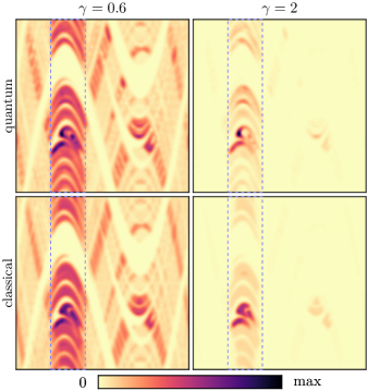
Figure 1: Average Husimi phase-space distribution of resonance eigenfunctions (top) compared to constructed classical measures $\mu_{\gamma}^{h}$ (bottom) with decay rates $\gamma=0.6$ (left) and $\gamma=2$ (right) for $h=1/1000$. Chaotic standard map with $\kappa=10$ on phase space $\Gamma=[0,1)\times[0,1)$ with opening $\Omega=[0.2,0.4]\times[0,1)$ (blue dashed line). Colormap with fixed maximum for each $\gamma$. Prominent localization for $\gamma=2$ and overall quantum-classical agreement.

For simplicity of the presentation we focus in the rest of the paper on time-discrete maps with chaotic dynamics and escape through an opening. The resulting discussion is straightforwardly generalized to autonomous systems like the paradigmatic three-disk scattering system or the Hénon-Heiles potential. Maps arise naturally, e.g., from a Poincaré section in autonomous systems or from a stroboscopic Poincaré section in time-periodically driven systems. Quantizing such a map yields a subunitary propagator whose non-orthogonal, right eigenfunctions have varying decay rates $\gamma$. Note that these eigenfunctions extend into the opening for the chosen ordering of escape before the mapping, see Fig. 1. Surprisingly, there occurs a localization of their average phase-space distribution within the opening. This localization is more prominent for resonance eigenfunctions with large decay rates $\gamma$, as visualized for the standard map (introduced below) in Fig. 1 (top). Thus, the following questions arise: What is the origin of this localization? What distinguishes the phase-space region of localization? More generally, is this effect caused by quantum interference (like dynamical localization Fis2010 or scarring due to periodic orbits Hel1984 ) or by properties of the classical dynamics?

Before answering these questions, let us briefly introduce the classical and quantum mechanical background. Classically, for chaotic dynamics of a map with escape almost all points on phase-space $\Gamma$ will be mapped into the opening $\Omega$ eventually and thus escape LaiTel2011 . Only a set of measure zero does not leave the system under forward and backward iteration. This invariant set usually is a fractal and is called the chaotic saddle $\Gamma_{\text{s}}$, see Fig. 2(a). Its unstable manifold consists of points approaching $\Gamma_{\text{s}}$ under the inverse map and is therefore called the backward-trapped set $\Gamma_{\text{b}}$, see Fig. 2(b). Generic initial phase-space distributions asymptotically converge to the uniform distribution on $\Gamma_{\text{b}}$, the so-called natural measure $\mu_{\text{nat}}$, with corresponding decay rate $\gamma_{\text{nat}}$ PiaYor1979 ; KanGra1985 ; Tel1987 ; LopMar1996 ; DemYou2006 ; AltPorTel2013 .

Quantum mechanically, the support of resonance eigenfunctions is given by the backward trapped set $\Gamma_{\text{b}}$ CasMasShe1999b ; KeaNovPraSie2006 . Furthermore, long-lived eigenfunctions with decay rates $\gamma\approx\gamma_{\text{nat}}$ are distributed as the natural measure $\mu_{\text{nat}}$ on phase space CasMasShe1999b , which corresponds to the steady-state distribution in the context of optical microcavities LeeRimRyuKwoChoKim2004 . There are a few supersharp resonances with $\gamma$ significantly smaller than $\gamma_{\text{nat}}$ Nov2012 . Instead, we focus on the large number of shorter-lived eigenfunctions ($\gamma>\gamma_{\text{nat}}$). For their integrated weight on $\Omega$ and on each of its preimages the dependence on the decay rate $\gamma$ was derived in reference KeaNovPraSie2006 . This concept is generalized by so-called conditionally invariant measures PiaYor1979 ; LopMar1996 ; DemYou2006 ; NonRub2007 . Recently, we suggested a specific conditionally invariant measure proportional to $\mu_{\text{nat}}$ on the opening $\Omega$, describing classically the weight of eigenfunctions on either side of a partial barrier KoeBaeKet2015 . None of these results, however, explains the observed localization phenomenon.

In this paper we propose a hypothesis for resonance eigenfunctions in chaotic systems predicting their average phase-space distribution. The hypothesis defines a conditionally invariant measure of the classical system for given decay rate $\gamma$ and effective Planck’s constant $h$. It gives a classical explanation for the localization of resonance eigenfunctions in those phase-space regions having the largest distance to the chaotic saddle. This is demonstrated in Fig. 1 for the chaotic standard map. We discuss the dependence on $\gamma$ and $h$, and briefly speculate about the semiclassical limit.

Resonance eigenfunction hypothesis.—We postulate that in chaotic systems with escape through an opening the average phase-space distribution of resonance eigenfunctions with decay rate $\gamma$ for effective Planck’s constant $h$ is described by a measure that $(i)$ is conditionally invariant with decay rate $\gamma$ and $(ii)$ is uniformly distributed on sets with the same temporal distance to the $h$-resolved chaotic saddle.

Combining both properties yields a measure

$$\mu_{\gamma}^{h}(A)=\frac{1}{\mathcal{N}}\int_{A}\text{e}^{t_{h}(x)\cdot(\gamma-\gamma_{\text{nat}})}\,\text{d}\mu_{\text{nat}}(x),$$ (1)

for all $A\subset\Gamma$ with normalization constant $\mathcal{N}$. Here the temporal saddle distance $t_{h}(x)\in\mathbb{R}$ fulfills

$$t_{h}(M^{-1}(x))=t_{h}(x)-1$$ (2)

for almost all $x\in\Gamma_{\text{b}}$, i.e. each backward iteration of the map $M$ on $\Gamma_{\text{b}}$ reduces the saddle distance by one. An important implication of Eq. (1) is that $\mu_{\gamma}^{h}$ is enhanced with increasing $\gamma>\gamma_{\text{nat}}$ in those regions of $\Gamma_{\text{b}}$ having the largest saddle distance, due to the exponential factor. These regions must be in the opening $\Omega$, which is easily shown by contradiction. Thus the hypothesis leads to a classical prediction for the localization of resonance eigenfunctions in chaotic systems.

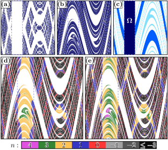
Figure 2: Classical sets for the considered standard map. (a) Chaotic saddle $\Gamma_{\text{s}}$, (b) backward trapped set $\Gamma_{\text{b}}$, (c) opening $\Omega$ and preimages $M^{-1}(\Omega),M^{-2}(\Omega)$ (from dark to light), (d, e) partition of the backward trapped set $\Gamma_{\text{b}}$ with colored sets $\mathcal{E}^{h}_{n}$ with integer saddle distance $n\leq m_{h}$ for (d) $h=1/1000$ with $m_{h}=3$ and (e) $h=1/16000$ with $m_{h}=4$. Regions with $n\leq 0$ are within the $h$-resolved saddle $\Gamma^{h}_{\text{s}}$.

We will now discuss properties $(i)$ and $(ii)$ in more detail. A measure $\mu$ is called conditionally invariant with decay rate $\gamma$ under a map $M$ with escape through an opening, if it is invariant under time evolution up to an overall decay,

$$\mu(M^{-1}(A))=\text{e}^{-\gamma}\,\mu(A),$$ (3)

for all $A\subset\Gamma$ PiaYor1979 ; LopMar1996 ; DemYou2006 . Equation (3) states that the set $M^{-1}(A)$, which consists of points that are mapped onto $A$, has a measure that is smaller by a factor $\text{e}^{-\gamma}$ than the measure of $A$. The support of conditionally invariant measures is the backward trapped set $\Gamma_{\text{b}}$. The most important of these measures is the natural measure $\mu_{\text{nat}}$ with decay rate $\gamma_{\text{nat}}$ LopMar1996 ; DemYou2006 . This measure is uniformly distributed on the backward trapped set $\Gamma_{\text{b}}$. We stress that for any decay rate $\gamma$ there are infinitely many different conditionally invariant measures DemYou2006 ; NonRub2007 . So far it is unknown, if any of these classical measures corresponds to resonance eigenfunctions with arbitrary decay rates.

Property $(ii)$ selects a specific class of measures which are uniformly distributed on subsets of $\Gamma_{\text{b}}$. Uniform distribution with respect to $\Gamma_{\text{b}}$ (the support of conditionally invariant measures) is equivalent to proportionality to the natural measure, explaining the appearance of $\mu_{\text{nat}}$ in Eq. (1). In analogy to quantum ergodicity for closed systems it is reasonable to consider for resonance eigenfunctions a uniform distribution on $\Gamma_{\text{s}}$, as classically this is an invariant set with chaotic dynamics. The quantum mechanical uncertainty relation, however, implies a finite phase-space resolution $h$ replacing $\Gamma_{\text{s}}$ by a quantum resolved saddle $\Gamma^{h}_{\text{s}}$. It is desirable to combine the assumption of uniformity on the saddle, the finite quantum resolution, and conditional invariance. This is achieved by introducing a temporal distance $t_{h}(x)$ to the quantum resolved saddle $\Gamma^{h}_{\text{s}}$ for all $x\in\Gamma_{\text{b}}$ and assuming uniformity on all sets with the same temporal distance. The resulting measures $\mu_{\gamma}^{h}$, Eq. (1), are conditionally invariant according to Eq. (3) as can be shown using Eq. (2).

For the saddle distance $t_{h}(x)$ we now provide a conceptually and numerically simple implementation. For this we consider as a convenient definition of $\Gamma^{h}_{\text{s}}$ a symmetric surrounding of $\Gamma_{\text{s}}$, $\Gamma^{h}_{\text{s}}=\{x\in\Gamma:d(x,\Gamma_{\text{s}})\leq\sqrt{\hbar/2}\}$, with Euclidean distance $d$ smaller than the width of coherent states. We define an integer saddle distance $n\in\mathbb{Z}$ for $x\in\Gamma_{\text{b}}$ as the number of backward steps to enter the $h$-resolved saddle,

$$t_{h}(x)=n\ \,\Leftrightarrow\ \,M^{-n}(x)\in\Gamma^{h}_{\text{s}},$$ (4)

with $M^{-i}(x)\notin\Gamma^{h}_{\text{s}}$ for all $i<n$. For points inside of $\Gamma^{h}_{\text{s}}$ this leads to $n\leq 0$. Defining $\mathcal{E}^{h}_{n}:=\{x\in\Gamma_{\text{b}}:t_{h}(x)=n\}$ as the sets with integer saddle distance $n$ we obtain a partition of $\Gamma_{\text{b}}$ with $\mathcal{E}^{h}_{n}=M^{n}\mathcal{E}^{h}_{0}$. There is a maximal saddle distance $m_{h}$, and consequently the regions $\mathcal{E}^{h}_{n}$ with $n>m_{h}$ are empty sets. With this Eq. (1) simplifies to

$$\mu_{\gamma}^{h}(A) =\frac{1}{\mathcal{N}}\sum_{n=-\infty}^{m_{h}}\text{e}^{n(\gamma-\gamma_{\text{nat}})}\mu_{\text{nat}}(A\cap\mathcal{E}^{h}_{n}),$$ (5)

for all $A\subset\Gamma$, which will be applied in the following.

Example system.—Throughout this paper we use the paradigmatic example of the standard map Chi1979 in its symmetric form $(q,p)\mapsto(q+p^{\ast},p^{\ast}+v(q+p^{\ast}))$ with $p^{\ast}=p+v(q)$ and $v(q)=(\kappa/4\pi)\sin(2\pi q)$, considered on the torus $q\in[0,1)$, $p\in[0,1)$ with periodic boundary conditions. We consider a kicking strength $\kappa=10$ to ensure a fully chaotic phase space. The opening is chosen as a vertical strip $\Omega$, such that $q\in[0.2,0.4]$ and $p\in[0,1)$, see Fig. 1. Position and size of $\Omega$ determine the classical decay rate $\gamma_{\text{nat}}\approx 0.21$ of the natural measure $\mu_{\text{nat}}$.

We consider the Floquet quantization $U_{\text{cl}}$ BerBalTabVor1979 ; ChaShi1986 of the closed map on a Hilbert space of dimension $1/h$ with effective Planck’s constant $h$. The quantum map is opened as $U=U_{\text{cl}}\cdot(\mathbbm{1}-P_{\Omega})$ with projector $P_{\Omega}$ on the opening BorGuaShe1991 . The eigenvalue problem of this subunitary propagator, $U\psi=\lambda\,\psi$, leads to eigenvalues with modulus less than unity, $|\lambda|^{2}\equiv\text{e}^{-\gamma}<1$. The decay rate $\gamma$ characterizes the time evolution of the corresponding resonance eigenfunction $\psi$. There is a broad distribution of decay rates $\gamma$ BorGuaShe1991 ; SchTwo2004 . We compute the Husimi phase-space distribution $\mathcal{H}(q,p)=1/h\ |\langle q,p|\psi\rangle|^{2}$ for each eigenfunction $\psi$ by taking the overlap with symmetric coherent states $|q,p\rangle$ centered at $(q,p)\in\Gamma$.

While Husimi distributions $\mathcal{H}$ of individual resonance eigenfunctions show strong quantum fluctuations, we want to explain their average behavior. Therefore we calculate the average Husimi distribution $\langle\mathcal{H}\rangle_{\gamma}$, where the average is taken over eigenfunctions from the interval $[{\gamma}\cdot c,{\gamma}/c]$ around some $\gamma$-value of interest with constant $c=0.95$. We improve this averaging by increasing the number of contributing Husimi distributions in two ways: First, we vary the Bloch phase $\theta_{p}\in\{0.04,0.08,\dots,0.96\}$ of the quantization $U$. Secondly, the inverse Planck’s constant is varied in $\{0.94,0.96,0.98,1,1.02,1.04,1.06\}\cdot h^{-1}$ for $h=1/1000$.

Classical measures $\mu_{\gamma}^{h}$ are obtained as follows. Using the sprinkler method LaiTel2011 we approximate the chaotic saddle $\Gamma_{\text{s}}$ as a point set with more than $10^{7}$ points not leaving the system under ten forward and backward time steps, see Fig. 2(a). Tenfold forward iteration of this set gives an approximation of $\Gamma_{\text{b}}$, see Fig. 2(b). The uniform distribution on this point set approximates $\mu_{\text{nat}}$ which is used in Eq. (5). We partition $\Gamma_{\text{b}}$ into sets $\mathcal{E}^{h}_{n}$ by determining the integer saddle distance $n$ for each $x\in\Gamma_{\text{b}}$, such that $d(M^{-n}(x),\Gamma_{\text{s}})\leq\sqrt{\hbar/2}$ and $d(M^{-n+1}(x),\Gamma_{\text{s}})>\sqrt{\hbar/2}$, shown in Figs. 2(d) and (e) for two values of $h$. Note that the region with maximal saddle distance $m_{h}$ is similar for both considered $h$. The saddle distance $n$ varies for points on $\Gamma_{\text{b}}$ and in particular on the opening $\Omega$ for two reasons: the geometric distance along the manifold to the quantum resolved saddle $\Gamma^{h}_{\text{s}}$ and the variation of the local stretching, i.e. finite time Lyapunov exponents. In order to construct $\mu_{\gamma}^{h}$, we assign to each $x\in\Gamma_{\text{b}}$ a weight $\text{e}^{n(\gamma-\gamma_{\text{nat}})}$ according to the factor in Eq. (5). Integrating these weights over grid cells with chosen resolution $800\times 800$ and normalizing we obtain a phase-space density numerically approximating $\mu_{\gamma}^{h}$.

Comparison.—In Fig. 1 we show the average phase-space distributions $\langle\mathcal{H}\rangle_{\gamma}$ for $\gamma=0.6$ and $\gamma=2$ for $h=1/1000$. Because $\mathcal{H}(q,p)$ is the expectation value of the projector on a coherent state $|q,p\rangle$, we compute the classical analogue. This is obtained by a convolution of the constructed measures $\mu_{\gamma}^{h}$ with a Gaussian of the same width as the coherent state, i.e. with standard deviation $\sqrt{\hbar/2}$. This allows for quantum-classical comparison on the phase space. Overall we observe very good agreement concerning the support of the distributions, their weight on the opening $\Omega$, and their localization within $\Omega$.

The Husimi distributions show the following features: First, they are supported by the smoothed backward trapped set. Secondly, one observes that their density on the opening $\Omega$ is larger than on its surrounding. The other stripes with larger density (than their surrounding) fall on the preimages $M^{-1}(\Omega)$ and $M^{-2}(\Omega)$, shown in Fig. 2(c). Thirdly and most importantly, the Husimi distributions within $\Omega$ are not uniform on $\Gamma_{\text{b}}$, but show localization, which is stronger for larger $\gamma$.

The same three observations hold for the constructed measures $\mu_{\gamma}^{h}$, where they directly follow from properties $(i)$ and $(ii)$. The first two observations are implied by conditional invariance. Note that the integrated weight on $\Omega$ increases with $\gamma$ as $\mu_{\gamma}^{h}(\Omega)=1-\text{e}^{-\gamma}$, which follows from Eq. (3). It also implies for the $k$-th preimage of the opening $\mu_{\gamma}^{h}(M^{-k}(\Omega))=\text{e}^{-k\gamma}\mu_{\gamma}^{h}(\Omega)$, which agrees with the quantum mechanical analysis KeaNovPraSie2006 . For the third observation we explicitly need the saddle distance in our classical construction, which follows from property $(ii)$. Those parts of $\Omega$ with maximal saddle distance $m_{h}$, see Fig. 2(d), show the largest enhancement due to the exponential factor in Eq. (5). Consequently, regions with smaller saddle distance are less enhanced. In conclusion we have found a classical explanation for the localization of resonance eigenfunctions. In particular, this shows that it is not an interference effect.

Note that our previously proposed measures KoeBaeKet2015 , which do not depend on $h$, only resemble the first two observations, but not the localization effect within the opening. Thus those measures fail to describe resonance eigenfunctions on a detailed level.

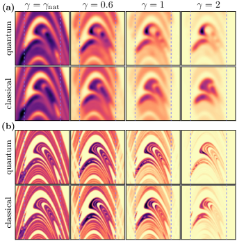
Figure 3: Average Husimi distribution of resonance eigenfunctions (top) compared to constructed classical measures $\mu_{\gamma}^{h}$ (bottom) with $\gamma\in\{\gamma_{\text{nat}},0.6,1,2\}$ for (a) $h=1/1000$ and (b) $h=1/16000$ on phase-space region $[0.15,0.45]\times[0.15,0.45]$. Colormap as in Fig. 1, with fixed maximum for each $\gamma$ in (a) and in (b).

Dependence on $\gamma$.—In Fig. 3(a) we illustrate quantum (top) and classical (bottom) phase-space distributions zoomed into the phase-space region $(q,p)\in[0.15,0.45]\times[0.15,0.45]$ for increasing decay rates $\gamma$ starting with $\gamma_{\text{nat}}$ for $h=1/1000$. This region is chosen to contain the significant peaks in $\Omega$. As expected, at the natural decay rate $\gamma_{\text{nat}}$ the Husimi distribution is almost perfectly resembled by the (smoothed) natural measure $\mu_{\text{nat}}$. Eigenfunctions with larger $\gamma$ show an increasingly prominent localization. Classically, this is reproduced using the measures (5). Note that at $\gamma=2$ also differences between classical and quantum densities can be seen. The main peak is sharper and stronger localized quantum mechanically than for the classical construction. We attribute this to the chosen simplification using an integer saddle distance.

Dependence on $h$.—Figure 3(b) shows the corresponding sequence of plots for much smaller effective Planck’s constant $h=1/16000$. The eigenfunctions resolve finer structures of the backward trapped set. Again, similarly good agreement between quantum and classical densities is found. In particular one observes stronger density variations on $\Gamma_{\text{b}}$ in form of arcs, e.g. for $\gamma=1$. Classically their origin is the increased maximum saddle distance $m_{h}=4$ and the finer partition of $\Gamma_{\text{b}}$ seen in Fig. 2(e) especially in the opening. Furthermore, the sets of maximal saddle distance $m_{h}$ are similar, see Figs. 2(d) and (e), such that the localization occurs in a similar region in Figs. 3(a) and (b). Again, at $\gamma=2$ sharper and stronger peaks occur in the quantum distribution than classically.

While numerically it is not possible to go to much smaller values of the effective Planck’s constant $h$, we briefly speculate about the semiclassical limit. Decreasing $h$ gives a smaller surrounding of $\Gamma_{\text{s}}$, such that the saddle distance $t_{h}(x)$ increases for all $x\in\Gamma_{\text{b}}$, including the maximum $m_{h}$. If for decreasing $h$ the difference $m_{h}-t_{h}(x)$ converges, one can show that the measures $\mu_{\gamma}^{h}$ converge towards a family of $\gamma$-dependent measures $\mu_{\gamma}$. In this case according to the hypothesis a semiclassical convergence of the eigenfunctions is expected.

If such limit measures $\mu_{\gamma}$ exist, it is a challenging question, whether and how they can be calculated directly. Moreover one would have to test, whether the structure of resonance eigenfunctions for finite $h$ is well enough explained by $\mu_{\gamma}$.

Discussion.—We have shown that the proposed resonance eigenfunction hypothesis for chaotic systems reproduces the average phase-space distribution of resonance eigenfunctions down to scales of order $h$. In particular the resulting measures $\mu_{\gamma}^{h}$ give a classical explanation of the quantum mechanically observed localization. Small deviations might be improved by more elaborate definitions of $\Gamma^{h}_{\text{s}}$ and the saddle distance $t_{h}(x)$, e.g. by considering in the definition of $\Gamma^{h}_{\text{s}}$ the distance along the unstable manifold or by considering continuous saddle distances from a smooth quantum resolved saddle. An application of the hypothesis to time-continuous systems, like open billiards and potential systems, is straightforward. A future challenge is the application to optical microcavities, which requires a generalization to partial transmission and reflection.

- (1) O. Bohigas, M. J. Giannoni, and C. Schmit: Characterization of Chaotic Quantum Spectra and Universality of Level Fluctuation Laws, Phys. Rev. Lett. 52 (1984), 1–4.
- (2) M. V. Berry: Semiclassical theory of spectral rigidity, Proc. R. Soc. Lon. A 400 (1985), 229–251.
- (3) M. Sieber and K. Richter: Correlations between periodic orbits and their rôle in spectral statistics, Phys. Scripta 2001 (2001), 128–133.
- (4) S. Müller, S. Heusler, P. Braun, F. Haake, and A. Altland: Semiclassical Foundation of Universality in Quantum Chaos, Phys. Rev. Lett. 93 (2004), 014103.
- (5) A. Voros: Semi-classical ergodicity of quantum eigenstates in the Wigner representation, in: Stochastic Behavior in Classical and Quantum Hamiltonian Systems (Eds. G. Casati and J. Ford), vol. 93 of Lecture Notes in Physics, 326–333, (Springer Berlin Heidelberg, Berlin), (1979).
- (6) M. V. Berry: Regular and irregular semiclassical wavefunctions, J. Phys. A 10 (1977), 2083–2091.
- (7) M. V. Berry: Semiclassical mechanics of regular and irregular motion, in: Comportement Chaotique des Systèmes Déterministes — Chaotic Behaviour of Deterministic Systems (Eds. G. Iooss, R. H. G. Helleman and R. Stora), 171–271, (North-Holland, Amsterdam), (1983).
- (8) A. I. Shnirelman: Ergodic properties of eigenfunctions (in Russian), Usp. Math. Nauk 29 (1974), 181–182.
- (9) Y. Colin de Verdière: Ergodicité et fonctions propres du laplacien (in French), Commun. Math. Phys. 102 (1985), 497–502.
- (10) S. Zelditch: Uniform distribution of eigenfunctions on compact hyperbolic surfaces, Duke. Math. J. 55 (1987), 919–941.
- (11) S. Zelditch and M. Zworski: Ergodicity of eigenfunctions for ergodic billiards, Commun. Math. Phys. 175 (1996), 673–682.
- (12) S. De Bièvre: Quantum chaos: a brief first visit, in: Second Summer School in Analysis and Mathematical Physics (Cuernavaca, 2000) (Eds. S. Pérez-Esteva and C. Villegas-Blas), Contemp. Math. 289, 161–218. Amer. Math. Soc., Providence, RI, (2001).
- (13) S. Nonnenmacher and A. Voros: Chaotic Eigenfunctions in Phase Space, J. Stat. Phys. 92 (1998), 431–518.
- (14) A. Bäcker, R. Schubert, and P. Stifter: Rate of quantum ergodicity in Euclidean billiards, Phys. Rev. E 57 (1998), 5425–5447, ; erratum ibid. 58 (1998) 5192.
- (15) M. Srednicki: Chaos and quantum thermalization, Phys. Rev. E 50 (1994), 888–901.
- (16) L. D’Alessio, Y. Kafri, A. Polkovnikov, and M. Rigol: From Quantum Chaos and Eigenstate Thermalization to Statistical Mechanics and Thermodynamics, Adv. Phys. 65 (2016), 239–362.
- (17) P. Gaspard: Quantum Chaotic Scattering, Scholarpedia 9(6): 9806, (2014).
- (18) G. E. Mitchell, A. Richter, and H. A. Weidenmüller: Random Matrices and Chaos in Nuclear Physics: Nuclear Reactions, Rev. Mod. Phys. 82 (2010), 2845–2901.
- (19) H.-J. Stöckmann: Quantum Chaos: An Introduction, (Cambridge University Press, Cambridge), (1999).
- (20) G. Tanner and N. Søndergaard: Wave Chaos in Acoustics and Elasticity, J. Phys. A 40 (2007), R443–R509.
- (21) R. A. Jalabert: Mesoscopic Transport and Quantum Chaos, Scholarpedia 11(1): 30946, (2016).
- (22) H. Cao and J. Wiersig: Dielectric microcavities: Model systems for wave chaos and non-Hermitian physics, Rev. Mod. Phys. 87 (2015), 61–111.
- (23) F. Haake, F. Izrailev, N. Lehmann, D. Saher, and H.-J. Sommers: Statistics of complex levels of random matrices for decaying systems, Z. Phys. B 88 (1992), 359–370.
- (24) Y. V. Fyodorov and H.-J. Sommers: Statistics of resonance poles, phase shifts and time delays in quantum chaotic scattering: Random matrix approach for systems with broken time-reversal invariance, J. Math. Phys. 38 (1997), 1918–1981.
- (25) Y. Alhassid: The statistical theory of quantum dots, Rev. Mod. Phys. 72 (2000), 895–968.
- (26) P. Jacquod, H. Schomerus, and C. W. J. Beenakker: Quantum Andreev Map: A Paradigm of Quantum Chaos in Superconductivity, Phys. Rev. Lett. 90 (2003), 207004.
- (27) Y. V. Fyodorov and D. V. Savin: Statistics of Resonance Width Shifts as a Signature of Eigenfunction Nonorthogonality, Phys. Rev. Lett. 108 (2012), 184101.
- (28) S. Kumar, B. Dietz, T. Guhr, and A. Richter: Distribution of Off-Diagonal Cross Sections in Quantum Chaotic Scattering: Exact Results and Data Comparison, Phys. Rev. Lett. 119 (2017), 244102.
- (29) J. Sjöstrand: Geometric Bounds on the Density of Resonances for Semiclassical Problems, Duke Math. J. 60 (1990), 1–57.
- (30) K. K. Lin: Numerical Study of Quantum Resonances in Chaotic Scattering, J. Comput. Phys. 176 (2002), 295–329.
- (31) W. T. Lu, S. Sridhar, and M. Zworski: Fractal Weyl Laws for Chaotic Open Systems, Phys. Rev. Lett. 91 (2003), 154101.
- (32) H. Schomerus and J. Tworzydło: Quantum-to-Classical Crossover of Quasibound States in Open Quantum Systems, Phys. Rev. Lett. 93 (2004), 154102.
- (33) S. Nonnenmacher and M. Zworski: Fractal Weyl laws in discrete models of chaotic scattering, J. Phys. A 38 (2005), 10683.
- (34) D. L. Shepelyansky: Fractal Weyl law for quantum fractal eigenstates, Phys. Rev. E 77 (2008), 015202.
- (35) J. A. Ramilowski, S. D. Prado, F. Borondo, and D. Farrelly: Fractal Weyl law behavior in an open Hamiltonian system, Phys. Rev. E 80 (2009), 055201.
- (36) M. Kopp and H. Schomerus: Fractal Weyl laws for quantum decay in dynamical systems with a mixed phase space, Phys. Rev. E 81 (2010), 026208.
- (37) M. J. Körber, M. Michler, A. Bäcker, and R. Ketzmerick: Hierarchical Fractal Weyl Laws for Chaotic Resonance States in Open Mixed Systems, Phys. Rev. Lett. 111 (2013), 114102.
- (38) H. Ishio, A. I. Saichev, A. F. Sadreev, and K.-F. Berggren: Wave Function Statistics for Ballistic Quantum Transport through Chaotic Open Billiards: Statistical Crossover and Coexistence of Regular and Chaotic Waves, Phys. Rev. E 64 (2001), 056208.
- (39) Y.-H. Kim, M. Barth, H.-J. Stöckmann, and J. P. Bird: Wave Function Scarring in Open Quantum Dots: A Microwave-Billiard Analog Study, Phys. Rev. B 65 (2002), 165317.
- (40) A. Bäcker, A. Manze, B. Huckestein, and R. Ketzmerick: Isolated resonances in conductance fluctuations and hierarchical states, Phys. Rev. E 66 (2002), 016211.
- (41) B. Weingartner, S. Rotter, and J. Burgdörfer: Simulation of Electron Transport through a Quantum Dot with Soft Walls, Phys. Rev. B 72 (2005), 115342.
- (42) T. Weich, S. Barkhofen, U. Kuhl, C. Poli, and H. Schomerus: Formation and interaction of resonance chains in the open three-disk system, New J. Phys. 16 (2014), 033029.
- (43) C. Gmachl, F. Capasso, E. E. Narimanov, J. U. Nöckel, A. D. Stone, J. Faist, D. L. Sivco, and A. Y. Cho: High-Power Directional Emission from Microlasers with Chaotic Resonators, Science 280 (1998), 1556–1564.
- (44) S.-Y. Lee, S. Rim, J.-W. Ryu, T.-Y. Kwon, M. Choi, and C.-M. Kim: Quasiscarred Resonances in a Spiral-Shaped Microcavity, Phys. Rev. Lett. 93 (2004), 164102.
- (45) J. Wiersig and M. Hentschel: Combining Directional Light Output and Ultralow Loss in Deformed Microdisks, Phys. Rev. Lett. 100 (2008), 033901.
- (46) S. Shinohara, T. Harayama, T. Fukushima, M. Hentschel, T. Sasaki, and E. E. Narimanov: Chaos-Assisted Directional Light Emission from Microcavity Lasers, Phys. Rev. Lett. 104 (2010), 163902.
- (47) J.-B. Shim, J. Wiersig, and H. Cao: Whispering gallery modes formed by partial barriers in ultrasmall deformed microdisks, Phys. Rev. E 84 (2011), 035202.
- (48) T. Harayama and S. Shinohara: Ray-Wave Correspondence in Chaotic Dielectric Billiards, Phys. Rev. E 92 (2015), 042916.
- (49) G. Casati, G. Maspero, and D. L. Shepelyansky: Quantum fractal eigenstates, Physica D 131 (1999), 311–316.
- (50) J. P. Keating, M. Novaes, S. D. Prado, and M. Sieber: Semiclassical Structure of Chaotic Resonance Eigenfunctions, Phys. Rev. Lett. 97 (2006), 150406.
- (51) S. Nonnenmacher and M. Rubin: Resonant eigenstates for a quantized chaotic system, Nonlinearity 20 (2007), 1387.
- (52) L. Ermann, G. G. Carlo, and M. Saraceno: Localization of Resonance Eigenfunctions on Quantum Repellers, Phys. Rev. Lett. 103 (2009), 054102.
- (53) D. Lippolis, J.-W. Ryu, S.-Y. Lee, and S. W. Kim: On-manifold localization in open quantum maps, Phys. Rev. E 86 (2012), 066213.
- (54) G. G. Carlo, D. A. Wisniacki, L. Ermann, R. M. Benito, and F. Borondo: Classical transients and the support of open quantum maps, Phys. Rev. E 87 (2013), 012909.
- (55) M. Schönwetter and E. G. Altmann: Quantum signatures of classical multifractal measures, Phys. Rev. E 91 (2015), 012919.
- (56) M. J. Körber, A. Bäcker, and R. Ketzmerick: Localization of Chaotic Resonance States due to a Partial Transport Barrier, Phys. Rev. Lett. 115 (2015), 254101.
- (57) S. Fishman: Anderson Localization and Quantum Chaos Maps, Scholarpedia 5(8): 9816, (2010).
- (58) E. J. Heller: Bound-State Eigenfunctions of Classically Chaotic Hamiltonian Systems: Scars of Periodic Orbits, Phys. Rev. Lett. 53 (1984), 1515–1518.
- (59) Y.-C. Lai and T. Tél: Transient Chaos: Complex Dynamics on Finite Time Scales, no. 173 in Applied Mathematical Sciences, (Springer Verlag, New York), 1st edn., (2011).
- (60) G. Pianigiani and J. A. Yorke: Expanding Maps on Sets Which Are Almost Invariant: Decay and Chaos, Trans. Amer. Math. Soc. 252 (1979), 351–366.
- (61) H. Kantz and P. Grassberger: Repellers, semi-attractors, and long-lived chaotic transients, Physica D 17 (1985), 75–86.
- (62) T. Tél: Escape rate from strange sets as an eigenvalue, Phys. Rev. A 36 (1987), 1502–1505.
- (63) A. Lopes and R. Markarian: Open Billiards: Invariant and Conditionally Invariant Probabilities on Cantor Sets, SIAM J. Appl. Math. 56 (1996), 651–680.
- (64) M. F. Demers and L.-S. Young: Escape rates and conditionally invariant measures, Nonlinearity 19 (2006), 377–397.
- (65) E. G. Altmann, J. S. E. Portela, and T. Tél: Leaking chaotic systems, Rev. Mod. Phys. 85 (2013), 869–918.
- (66) M. Novaes: Supersharp resonances in chaotic wave scattering, Phys. Rev. E 85 (2012), 036202.
- (67) B. V. Chirikov: A universal instability of many-dimensional oscillator systems, Phys. Rep. 52 (1979), 263–379.
- (68) M. V. Berry, N. L. Balazs, M. Tabor, and A. Voros: Quantum maps, Ann. Phys. (N.Y.) 122 (1979), 26–63.
- (69) S.-J. Chang and K.-J. Shi: Evolution and exact eigenstates of a resonant quantum system, Phys. Rev. A 34 (1986), 7–22.
- (70) F. Borgonovi, I. Guarneri, and D. L. Shepelyansky: Statistics of Quantum Lifetimes in a Classically Chaotic System, Phys. Rev. A 43 (1991), 4517–4520.