Exploring out-of-equilibrium quantum magnetism and thermalization in a spin-3 many-body dipolar lattice system

Abstract

Understanding quantum thermalization through entanglement build-up in isolated quantum systems addresses fundamental questions on how unitary dynamics connects to statistical physics. Here, we study the spin dynamics and approach towards local thermal equilibrium of a macroscopic ensemble of $S=3$ spins prepared in a pure coherent spin state, tilted compared to the magnetic field, under the effect of magnetic dipole-dipole interactions. The experiment uses a unit filled array of $\approx 10^{4}$ chromium atoms in a three dimensional optical lattice, realizing the spin-3 XXZ Heisenberg model. The build up of quantum correlation during the dynamics, specially as the angle approaches $\pi/2$, is supported by comparison with an improved numerical quantum phase-space method and further confirmed by the observation that our isolated system thermalizes under its own dynamics, reaching a steady state consistent with the one extracted from a thermal ensemble with a temperature dictated from the system’s energy. This indicates a scenario of quantum thermalization which is tied to the growth of entanglement entropy. Although direct experimental measurements of the Renyi entropy in our macroscopic system are unfeasible, the excellent agreement with the theory, which can compute this entropy, does indicate entanglement build-up..

Ultra-cold atomic systems featuring long-range interactions are becoming ideal platforms for probing strongly correlated out-of-equilibrium quantum behavior and, in particular, the phenomenon of quantum magnetism, where magnetic moments with quantized energy levels (spins) interact with one another Bohn2017 ; Blatt2012 ; Saffman2010 . Their appeal stems from the fact that they feature internal levels that can be initialized in pure states and coherently evolved with controllable long-range interactions even under frozen conditions. Recently great advances have been accomplished, but, so far have been mostly limited to small systems (hundreds or fewer particles) Bohnet2016 ; Garttner2017 ; Richerme2014 ; Jurcevic2014 ; Jurcevic2017 ; Hess2017 ; Zeiher2017 ; labuhn2016 ; Bernien2017 , or to dilute disordered molecular ensemblesYan2013 ; Hazzard2014b . Magnetic quantum dipoles featuring sizable magnetic moments offer unique opportunities since magnetic interactions can directly happen in an enlarged set of low-lying hyperfine Zeeman levels and are not forbidden by parity and time-reversal symmetry as is the case with electric dipolesLahaye2009 . They offer untapped opportunities as a quantum resource since $S>1/2$ spin models have more complexity and cost exponentially more resources to classically simulateAharonov2007 ; Hallgren2013 . In fact, the exploration of the complex non-equilibrium dynamics of dipolar-coupled $S>1/2$ spin models remains a fascinating territory which only starts to be explored depaz2013 ; depaz2016 . Here we make a step forward and report on experimental observations on how the seven Zeeman populations of an initial spin coherent state made of $S=3$ spin particles, evolve and at long times approach a steady state that is captured by a statistical ensemble with nonzero thermodynamic entropy, as a result of the entanglement accumulated during the dynamics.

In our system the spin degree of freedom is encoded in the Zeeman levels of the purely electronic $S=3$ ground state of ⁵²Cr atoms. The experiment starts with the production of a spin-3 Bose-Einstein condensate (BEC) of approximately $4\times 10^{4}$ atoms in the $m_{S}=-3$ state, following the procedure described in Ref. lepoutre2017 . We then adiabatically load the BEC into a three dimensional (3D) optical lattice made by laser beams at 532 nm depaz2013 . The lattice structure is rectangular in the horizontal plane, and uses a standard retro-reflecting scheme on the vertical axis (Methods). After loading the atoms into a deep optical lattice, the sample forms a Mott insulator consisting of a core with doubly-occupied sites ($\overline{n}=2$), surrounded by a 3D shell of singly occupied sites ($\overline{n}=1$), see Fig. 1.

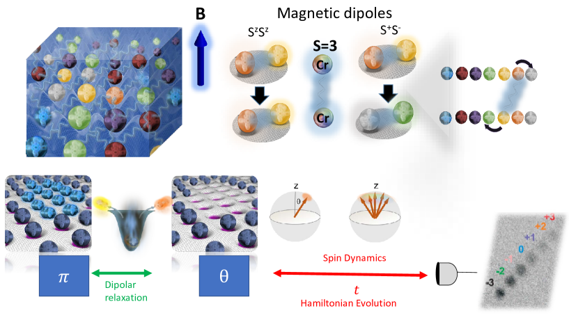
Figure 1: Sketch of the experiment. We consider an assembly of $S=3$ Cr atoms in an optical lattice prepared in a Mott-insulating state. Dynamics is driven by dipole-dipole interactions which feature both Ising ($\hat{S}_{i}^{z}\hat{S}_{j}^{z}$) and exchange ($\hat{S}_{i}^{+}\hat{S}_{j}^{-}+h.c$) terms. A first $\pi$ pulse is used to promote all atoms to the most excited spin state. Dipolar relaxation empties doubly occupied sites. Once this is achieved, a second pulse collectively rotates all spins by an angle $\theta$ from the $B$ field which sets the quantization direction. We then study spin dynamics due to intersite dipole-dipole interactions by registering the relative population of the different Zeeman states.

The experimental procedure to induce spin dynamics is shown in Fig. 1. We initialize the system in a well characterized state consisting of a macroscopic array of long-lived singly-occupied sites close to unit filling by performing first a filtering protocol. It relies on dipolar relaxation depaz2013 to empty all doubly-occupied sites within the $\overline{n}=2$ Mott core after the application of a $\pi$ rf-pulse that promotes the atoms to the most energetic spin state $m_{S}=3$. The filtering protocol takes about 7 ms (Methods). To trigger the spin dynamics we then apply a second rf pulse. This rotates the coherent spin state, such that it forms an angle $\theta$ with respect to the magnetic field which sets the quantization axis (see Fig. 1). This prepares a tilted spin coherent state. The spin dynamics is studied by monitoring the time evolution of the population of the different Zeeman states, using absorption imaging after a Stern Gerlach separation procedure lepoutre2017 .

A unit filled array of frozen magnetic dipoles in a lattice interact via dipolar exchange interactions. In the presence of a magnetic $B$ field strong enough to generate Zeeman splittings larger than nearest-neighbor dipolar exchange processes, only those processes that conserve the total magnetization are energetically allowed and the dynamics is described by the following secular Hamiltoniandepaz2013 :

$$\hat{H}=\sum_{i>j}^{N}V_{ij}\left[\hat{S}_{i}^{z}\hat{S}_{j}^{z}-\frac{1}{2}\left(\hat{S}_{i}^{x}\hat{S}_{j}^{x}+\hat{S}_{i}^{y}\hat{S}_{j}^{y}\right)\right]$$ (1)

where the sum runs over the $N$ populated singly-occupied lattice sites. It corresponds to a XXZ Heisenberg model with dipolar couplings $V_{i,j}\equiv\frac{\mu_{0}(g\mu_{B})^{2}}{4\pi}\left(\frac{1-3\cos^{2}\phi_{(i,j)}}{r_{(i,j)}^{3}}\right)$. Here $\mu_{0}$ is the magnetic permeability of vacuum, $g\simeq 2$ is the Landé factor, and $\mu_{B}$ the Bohr magneton. The sum runs over all pairs of particles ($i$,$j$). $r_{(i,j)}$ is the distance between atoms, and $\phi_{(i,j)}$ the angle between their inter-atomic axis and the external magnetic field. The Hamiltonian is given in terms of spin-3 angular momentum operators, ${\bf{\hat{S}}}_{i}=\{\hat{S}_{i}^{x},\hat{S}_{i}^{y},\hat{S}_{i}^{z}\}$ , associated to atom $i$.

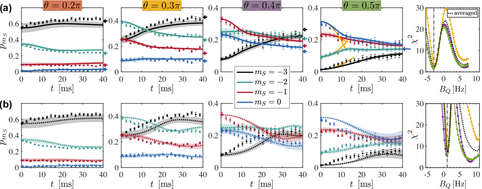
Figure 2: Comparison between classical and quantum dynamics of the four lowest spin-level populations, $p_{m_{S}}$, for various initial tilting angles $\theta=0.2\pi$, $0.3\pi$, $0,4\pi$, and $0.5\pi$. (a) Comparison of experimental data with GDTWA simulations (solid lines) on a $7\times 3\times 7$ cluster allowing the quadratic Zeeman field $B_{Q}$ to be the only fitting parameter [here: $B_{Q}=-3.0\,\text{Hz}$]. (b) Comparison of the experiment with the classical mean-field results (dotted lines) [here: $B_{Q}=1.1\,\text{Hz}$]. The two plots on the right show quantitative comparison between data and simulations for $\theta=0.3\pi$, $0,4\pi$, and $0.5\pi$ with a reduced $\chi^{2}$ criteria, for different values of $B_{Q}$. We excluded the $\theta=0.2\pi$ case here since it shows no significance dynamics. The best agreement with GDTWA simulations is a factor of three better than with classical simulations. The deviation with the classical simulations is most obvious at short times, and clearly increases with increasing $\theta$. The thick arrows indicate the expected equilibrium population maximizing entropy, for each angle. The red solid line in panel (a) (for $\theta=0.5\pi$) is the result of the perturbative expansion, Eq.(3). The shaded area indicates the range of variation of the populations for evolutions with $\Delta B_{Q}=\pm 0.3\,\text{Hz}$ and uncertainties in the tilting angles with $\theta=(0.2\pm 0.018\pi),(0.3\pm 0.012)\pi,(0.4\pm 0.012)\pi,(0.5\pm 0.01)\pi$ (estimated from the experiment).

An important feature is that the dynamical redistribution of populations can happen for large spins ( $S>1/2$), even though both the total particle number $N$ and the collective magnetization $M=\langle\hat{S}^{z}\rangle$ are conserved quantities (with $\hat{S}^{x,y,z}=\sum_{j=1}^{N}\hat{S}_{i}^{x,y,z}$). The magnetic dipolar interaction energy between $S=3$ spins is 36 times larger than the one for $S=1/2$ alkali atoms, allowing us to probe such population dynamics at milliseconds time scales, as seen in Fig 2.

We will first introduce the expected basic dynamical features according to time-dependent perturbation theory. We will focus on the main differences when assuming a classical behavior, or when taking into account quantum correlations. The simplest possible picture for the population dynamics relies on a mean field treatment( $i.e.$ neglecting quantum correlations), where each atom undergoes Larmor precession around an effective dipolar field created by all the other spins, $\hat{H}^{MF}=\sum_{i=1}^{N}{\bf B}^{\rm eff}_{i}\cdot{\bf\hat{S}}_{i}$, with ${\bf B}^{\rm eff}_{i}=-\sum_{j=1}^{N}\frac{V_{ij}}{2}\{\langle\hat{S}_{j}^{x}\rangle,\langle\hat{S}_{j}^{y}\rangle,-2\langle\hat{S}_{j}^{z}\rangle\}$. Time-dependent perturbation theory yields the following equation for $p_{m_{S}}$, the relative population of Zeeman level $m_{S}=-3,\dots,3$:

$$p_{m_{S}}^{\rm MF}(t)=p_{m_{S}}(0)+\sin[\theta]^{4}\alpha_{m_{S}}(\theta)t^{2}{\mathcal{K}}_{d}(t)+\mathcal{O}\Big{(}t^{6}V_{ij}^{6}\Big{)},$$ (2)

We give in Methods exact formulas for $\alpha_{m_{S}}(\theta)$. For instance, $\alpha_{m_{S}=\{-3,-2,-1,0,1,2,3\}}(\pi/2)=135/512\times\{1,2,-1,-4,-1,2,1\}$. Here ${\mathcal{K}_{d}}(t)\equiv\frac{t^{2}}{2N}\sum_{i=1}^{N}\left[\sum_{j\neq i}^{N}V_{ij}B^{dih}_{ij}\right]^{2}$. Thus classical dynamics is driven by the dipolar field $B^{dih}_{ij}=-9/2\sum_{k\neq j,i}^{N}(V_{ki}-V_{kj})\cos\theta$. For a homogeneous gas, $B^{dih}$ vanishes, and the population dynamics with it. This behavior remains valid at all times given that, by preparation, all spins point along the same direction initially, they precess around the same classical dipolar field, and thus evolve identically. Therefore, the local magnetization $\langle S_{i}^{z}\rangle=M/N$ remains constant for each spin, canceling population dynamics altogether. On the other hand, in a trapped gas, the inhomogeneous dipolar field introduces a differential precession rate between spins, which results in population dynamics. Note that $B^{dih}$ is determined by border effects and also that ${\mathcal{K}_{d}}(t)$ itself is time dependent ($\propto t^{2}$). Therefore, classically, population redistribution is a slow $t^{4}$ process. We emphasize that $B^{dih}$ is proportional to $\cos\theta$ and thus vanishes when $\theta=\pi/2$ where no mean-field dynamics takes place at all.

Quantum fluctuations can drastically modify this behavior and induce much faster population dynamics even for a homogeneous gas Hazzard2013 . Second-order time-dependent perturbation theory on the exact HamiltonianNMRbook ; Hazzard2014a (Eq. 1) yields:

$$p_{m_{S}}(t)=p_{m_{S}}(0)+\sin[\theta]^{4}\alpha_{m_{S}}(\theta)t^{2}V_{\rm eff}^{2}+\mathcal{O}\Big{(}t^{4}V_{ij}^{4}\Big{)}.$$ (3)

In contrast to the mean field case, the dynamics grows as $t^{2}$ and is driven by $V_{\rm eff}\equiv\sqrt{\sum_{i,j\neq i}^{N}V_{ij}^{2}/N}$. We emphasize the relative fast decay of $V_{\rm eff}^{2}$ with interparticle distance $r$ (as $r^{-6}$), which makes the short time evolution mainly determined by the nearest-neighbor interactions. As $V_{\rm eff}$ is independent of $\theta$ the tipping angle $\theta$ provides us a way to study an out-of-equilibrium magnetism increasingly determined by quantum correlations as $\theta\rightarrow\pi/2$.

In the experiment, external systematics such as quadratic Zeeman fields, $B_{Q}$, generated by tensorial light shifts induced by the lattice lasers –with eigenenergies $B_{Q}m_{S}^{2}$– or inhomogeneities associated to magnetic field gradients, $\Delta_{ij}=B_{i}-B_{j}$ need to be accounted for. Their role on the short time dynamics can be understood using perturbation theory (Methods). Quadratic Zeeman fields can be accounted for by replacing ${\mathcal{K}}_{d}(t)\to{\mathcal{K}}_{d}(t)-4/3Q^{2}$ and $V_{\rm eff}^{2}\to V_{\rm eff}^{2}-4/3Q^{2}$ in the classical and quantum cases respectively, with $Q^{2}\equiv\frac{1}{N}\sum_{j\neq i}^{N}V_{ij}B_{Q}$. At the mean-field level $\Delta_{ij}$ directly renormalizes $B^{dih}_{ij}\to B^{dih}_{ij}+\Delta_{ij}$. Thus dipolar inhomogeneities and magnetic field gradients are in direct competition. In the quantum case, magnetic field gradients also enter as $t^{4}$ but in this case they play a subdominant role since the leading dipolar dynamics is significantly faster ($\propto t^{2}$).

Although perturbation theory allows emphasizing some of the main qualitative differences in the classical and in the quantum regime, to accurately describe the population dynamics we need to go beyond perturbation theory. To accomplish that we parameterize each spin $i$ by a generalized Bloch vector, $\vec{\lambda}^{[i]}$. In contrast to spin-1/2 systems, this vector is a 48-dimensional object that determines all independent elements of the $7\times 7(=(2S+1)^{2})$ individual spin-3 density matrices, $\hat{\rho}_{i}(\vec{\lambda}^{[i]})$, Bertlmann2008 . Inserting the product state ansatz of the system density matrix, $\hat{\rho}=\prod_{i=1}^{N}\hat{\rho}_{i}(\vec{\lambda}^{[i]})$, into the von Neumann equation, $d\hat{\rho}/dt=(-{\rm i}/\hbar)[H,\hat{\rho}]$ , yields $N\times 48$ independent non-linear mean field equations, in which each generalized Bloch vector evolves in the field of the others (Methods and Supplementary material). The mean field “classical” results are obtained by numerically integrating these equations of motion.

To capture the build up of quantum correlations we developed a generalization of a semiclassical method (generalized discrete truncated Wigner approximation, GDTWA) based on a discrete Monte Carlo sampling in phase space originally derived in the framework of the so-called truncated Wigner approximation (TWA)Polkovnikov . It describes the initial state in terms of a probability distribution. Initial spin coherent states are ideal since they can be fully described by a positive discrete probability distribution. For spin-1/2 systems, randomly sampling this initial “Wigner function”, leads to the discrete truncated Wigner approximation (DTWA) Schachenmayer2015a ; Schachenmayer2015b ; Orioli2017 , an approximation that has been remarkably successful and can capture complex quantum aspects of spin-dynamics. In contrast to the spin-1/2 case, here (GDTWA) the discrete probabilities are not provided by the eigenvalues of the three Pauli matrices, but instead by the eigenvalues of the corresponding 48 generalized SU(7) generators (Methods).

We now describe how our data compares with simulations for different values of $\theta$. In Fig. 2 we show our data and the comparisons to both the classical and the GDTWA models. The theoretical models take into account the 3D lattice structure and the measured magnetic field gradients along all three directions. We also include the weak quadratic Zeeman field present in the experiment. Since we cannot measure it directly we allow it to be a fitting parameter; For each of the four tilting angles used for the measurements we plot the evolution of fractional populations in different Zeeman states. We only plot the most relevant Zeeman states (the most populated for most of the angles, and only the negative Zeeman states for the symmetric case $\pi/2$). Experimentally, we find that the amplitude of spin dynamics (i.e. the amplitude of the variations of the populations in the different spin states) is stronger when the angle increases.

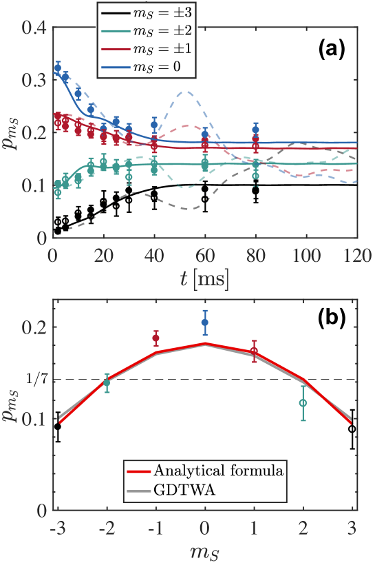
Figure 3: Quantum Thermalization. (a) Long-time evolution of state populations for $\theta=\pi/2$: Long time experimental data points are compared to corresponding best fitting GDTWA (solid lines, $B_{Q}\approx-3.6\,$Hz) and mean-field (thin dashed lines, $B_{Q}\approx 1.1\,$Hz). (b) The experimental data points at $t=80\,$ ms are compared to the GDTWA prediction (including field gradients), and the analytical quantum thermalization expression, Eq.5, which corresponds to an effective temperature of $-2.5\,$nK, using $B_{Q}=-3.6\,$Hz.

At small angles the experimental data is qualitatively reproduced by both classical and GDTWA simulations. As can be seen in Fig. 2, both simulations then yield similar results, but nevertheless show systematic differences. This shows that even at the smallest angles that we have probed, beyond mean-field effects are in principle already at play. However, given the signal-to-noise ratio in the experimental data, it is difficult to quantify the contribution of beyond mean field effects to the spin dynamics at weak rotations. When increasing the angle, it becomes increasingly clear that only the beyond mean-field simulation accounts for the observed dynamics, both at short times ($t<20$ ms, see Fig 2), and at long times ($t>40$ ms, see Fig 3a)).

We have performed a systematic study in our numerical simulations, by varying the size of the system which we use. We find that a good agreement between experiment and beyond mean-field theory is only reached provided the number of interacting spins in the simulation is larger than about 60. Taken together, these data show that spin dynamics after the initial quench is inherently many-body, and beyond the grasp of mean-field models. As can also be seen in Fig. 2, our experimental data at short times is also in excellent agreement with the exact dynamics calculated within the framework of second-order time-dependent perturbation theory (see Eq. (3)). Also in good agreement with this equation, we find the dynamics at short times to be roughly independent of the magnetic field gradient applied to the sample (up to values $>30$ MHz$/$m). In contrast, we point out that the experimental data at short times systematically shows faster dynamics than predicted in the classical picture, whose initial $t^{4}$ dependence (See Eq. 2) fails reproducing the experimental observations.

For an isolated system, entanglement build-up after a quench into a non-equilibrium situation is tied to the scenario of quantum thermalization. To support the relevance of quantum correlations during dynamics, we thus analyze the long time behavior of the populations. For all tipping angles $\theta$, we observe that the experimental system approaches a steady state, which is in agreement with predictions of closed system quantum thermalization, given e.g. by the Eigenstate Thermalization Hypothesis (ETH) Alessio2016 ; Kaufman2016 . In particular, we find that the long-time average populations are very well described by the effective thermal distribution $\hat{\rho}_{cT}(\beta,\mu)=\frac{e^{-\beta{\hat{H}}_{T}-\mu{\hat{S}}^{z}}}{{\rm tr}[e^{-\beta{\hat{H}}_{T}-\mu\hat{\hat{S}}^{z}}]}$ where the chemical potential $\mu$ and inverse temperature $\beta=1/k_{B}T$ are set by the energy and magnetization of the initial pure state:

$$\langle\hat{H_{t}}\rangle={\rm tr}[\hat{\rho}_{cT}(\beta,\mu)\hat{H_{T}}]\quad\quad\langle\hat{S}^{z}\rangle={\rm tr}[\hat{\rho}_{cT}(\beta,\mu)\hat{S}^{z}],$$ (4)

which are conserved throughout the evolution. Here $\hat{H}_{T}=\hat{H}+\sum_{i}B_{Q}(\hat{S}_{i}^{z})^{2}$ is the total Hamiltonian. As shown in Fig 2 the steady state populations approach the ones (indicated by the arrows for all tipping angles) dictated by the thermal ensemble when simply setting $\beta=0$ (in which case the maximum entropy state only depends on magnetization). For angles close to $\pi/2$, however, where quantum effects are most significant, we find a deviation compared to this simplistic prediction. We therefore proceed to study this interesting regime.

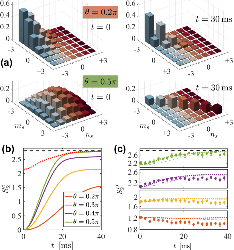
Figure 4: Entanglement build-up (a) Absolute values of the central spin density-matrix elements $|\rho^{c}_{m_{S},n_{S}}|$ with $\rho^{c}_{m_{s},n_{S}}\equiv\langle m_{S}|\hat{\rho}_{0}|n_{S}\rangle$, extracted from GDTWA simulations with the same parameters as in Fig. 2. Off-diagonal single-site coherences are destroyed as the spins become entangled during the quantum dynamics (left two panels: $t=0$, after the tilt, right two panels: after $t=30\,\text{ms}$ evolution). For small rotation angles (upper panels: $\theta=0.2\pi$), the system evolves locally into a partially mixed state (un-even spin-state population). For larger rotation angles (lower panels: $\theta=0.5\pi$), the local state resembles a maximally mixed state of the form $\hat{\rho}_{0}\propto\frac{1}{7}\sum_{m_{S}=-3}^{3}|m_{S}\rangle\langle m_{S}\rangle$. (b) Evolution of $S^{c}_{2}$, the value of the second order Renyi-entropy $S^{(2)}_{0}$ for the central spin density matrix. For larger rotation angles, the entanglement entropy increases with time, almost reaching the maximum value ($S^{(2){\rm max}}_{0}\leq\log_{2}(7)$, black dashed line). The red dotted line shows the upper bound $S_{2}^{D}$, computed only from the diagonal elements (populations) of the average single site density matrix $\hat{\rho}_{S}$ (see text) for $\theta=0.5\pi$. (c) Comparison of the theoretically computed diagonal entropy (GDTWA: thick dotted line; mean-field: thin dashed line) with the one reconstructed from the measured populations.

In Fig. 3 we show dynamics up to longer times, and confirm the steady state is indeed reached after 40 ms for the $\pi/2$ case, a feature that the GDTWA simulation reproduces, while classical simulations predict an oscillatory behavior for a much longer duration. This qualitative difference between the classical and the quantum behavior is associated with the different origin of thermalization in both pictures: while quantum-mechanically thermalization is tied to the growth of entanglement, classically, reaching a steady state in a system of frozen particles is a consequence of the single particle dephasing in precession induced by field inhomogeneities (which differs from the typical thermalization scenario in mobile particles where collisions can classically redistribute energies and momenta Alessio2016 ; Weiss ; Langen207 ; lev2018 ). Our observations clearly rule out a simple mean-field (classical) behavior. Most interestingly, we find a very good agreement between the experimental data points taken at long times, i.e. after the system has reached its steady state, if instead of setting $\beta=0$ we account for the corrections generated by the quadratic Zeeman field $B_{Q}$, and the finite but small energy of the initial state in Eq. (4). Using a simple perturbative approach (see Methods and Supplementary material) we obtain that the $\beta^{(0)}=\mu^{(0)}=0$ solutions should be replaced by:

$$\beta^{(1)} = \frac{{\rm tr}[\hat{\rho}_{cT}(0,0)\hat{H}_{T}]-\langle\hat{H_{T}}\rangle}{{\rm tr}[\hat{\rho}_{cT}(0,0)\hat{H}_{T}^{2}]-{\rm tr}[\hat{\rho}_{cT}(0,0)\hat{H}_{T}]^{2}}$$

$$= \frac{5B_{Q}+9\bar{V}}{24V_{\rm eff}^{2}+24B_{Q}^{2}},$$

$$p_{m_{S}}(t_{SS}) \approx {\rm tr}[\hat{\rho}_{cT}(\beta^{(1)},0){\hat{p}}_{m_{S}}]=\frac{1}{7}\big{(}1-\beta^{(1)}B_{Q}(m_{S}^{2}-4)\big{)},$$

$$\mu^{(1)}=0$$ (5)

with $\bar{V}\equiv 1/N\sum_{i>j}^{N}V_{ij}$. We find $\bar{V}/h\approx-0.57$ Hz and $V_{\rm eff}/h\approx 6.13$ Hz for our lattice geometry. As $\bar{V}<0$, negative temperatures are expected for low enough $B_{Q}$ (as allowed for a system whose maximum energy is bounded). Fig. 3b) shows a very good agreement between the equilibrium data and the analytical model. For this comparison, there is no free parameter, since we use the value of $B_{Q}$ for which the dynamical evolution of the spins is best reproduced by GDTWA simulations. This good agreement confirms the scenario that the coherent Hamiltonian evolution of the many-body system drives it towards a strongly entangled pure state for which the observables display thermal-like behavior. The agreement between the analytical model and the GDTWA at long times shown in Fig. 3b) also indicates that the GDTWA not only captures the short term dynamics (as previously known from the theoretical point of view), but also the approach to equilibrium.

To compare the analytical formula to the data we have ignored magnetic field gradients in Eq. (5). In principle, magnetic field gradients should lead to an equilibrium state where a spatial texture of magnetization develops. However, such a texture requires long-range interactions between remote parts of the cloud, which only occurs for an extremely long time-scale for dipolar interactions. We have verified (see Supplementary material) that indeed magnetic field gradients can be neglected to evaluate the quasi-steady state populations reached at 100 ms. This shows that a local equilibrium is first reached, well before the full many-body system may reach true equilibrium with maximum entropy, where all populations in the different Zeeman states would be equally populated.

To further quantify the importance of quantum correlations in the spin dynamics as a function of the tilting angle $\theta$, we analyze from the theoretical point of view the properties of the reduced density matrix for each spin, $\hat{\rho}_{i}(\vec{\lambda}^{[i]})$. In our simulations those density matrices are readily available from the generalized Bloch vectors. To minimize finite size and boundary effects we focus on the density matrix of the central spin of our simulated block $\hat{\rho}_{0}$. Even when, as in our simulations, the quantum state of the full system $\hat{\rho}$ is pure, the reduced single spin density matrices can assume a mixed character due to the build up of entanglement between the spins. This mixed character is quantified by a reduced purity, ${\rm tr}(\hat{\rho}_{0}^{2})<1$ and thus an increased entropy, which we compute in terms of the second-order Renyi entropy, $S_{0}^{(2)}=-\log_{2}[{\rm tr}(\hat{\rho}_{0}^{2})]$. If the state of the full system is pure, ${\rm tr}(\hat{\rho}^{2})=1$, the Renyi entropy is a measure of entanglement Renyi : it is zero for product states, and reaches the maximum value of $S_{0}^{(2){\rm max}}=\log_{2}[7]$ (the value for a fully mixed state of a spin-3 particle) for many-body states where the quantum information encoded in an individual spin is completely scrambled due to entanglement with other ones.

As can be seen in Fig. 4, the quantum evolution leads to a growth of $S_{0}^{(2)}$ already for the smallest investigated angle $\theta=0.2\pi$. The dynamical growth of entanglement increases significantly for larger tilt angles. At $\theta=\pi/2$, we find that $S_{0}^{(2)}$ approaches its maximum possible value $S_{0}^{(2)\rm{max}}$. Although we cannot perform a full state-tomography from the experimental data, we can compare our experimental data to a “diagonal entropy” computed in terms of the diagonal part of the averaged single particle density matrix $\hat{\rho}_{S}=(1/N)\sum_{i=1}^{N}\hat{\rho}_{i}(\vec{\lambda}^{[i]})$. Note that for an homogeneous system $\hat{\rho}_{S}=\hat{\rho}_{0}$. By neglecting the off-diagonal coherences of $\hat{\rho}_{S}$ we can define this entropy as $S_{2}^{D}=-\log_{2}\{{\rm tr}[{\rm diag}(\hat{\rho}_{S})^{2}]\}$, which can be readily accessed from the population data, assuming homogeneity: $S_{2}^{D}=-\log_{2}\{\sum p_{m_{S}}^{2}\}$.

This diagonal entropy is not an entanglement witness, but it provides an upper bound of the entanglement entropy, $S_{2}^{D}\geq S_{0}^{(2)}$. In a translationally invariant system it increases as quantum correlations build up with time and approaches the full entropy as the single-spin density matrices decohere due to entanglement. However, in our finite system, boundary effects can obscure this behavior. Although this is the case at small angles, where diagonal entropy shows a slight reduction as a function of time, as can be seen in Fig. 4 for $\theta\geq 0.3\pi$ we do observe it increases with time as the system thermalizes. The non-trivial growth of the experimental diagonal entropy is in excellent agreement with our theoretical estimates, provided quantum fluctuations are taken into account. Moreover it also approaches $S_{0}^{(2)}$ for $\theta=\pi/2$.

In summary our study demonstrates the dominant role of quantum correlations in the out-of-equilibrium dynamics of an initially uncorrelated spin coherent state, when the angle it makes with the magnetic field is close to $\pi/2$. Our system is the first example of a long-range interacting many-particle isolated spin system which internally thermalizes through entanglement build-up, and develops an effective thermal-like behavior through a mechanism which is purely quantum and conservative. The comparison between experiment and theory shows that the GDTWA simulations can be trusted for studying the dynamics in a complex quantum many-body system, provided a sufficient number of atoms is included in the simulation. Thus, our experiment provides a test-bed for a new theoretical method based on the GDTWA, for the first time applied to systems of large spins, and in a many-body regime where simulations based on exact diagonalization techniques are intractable with current computational resources. In turn, our study can be used as a first benchmark of a quantum simulator of the spin-3 XXZ Heisenberg model and opens a path towards the study of open problems in quantum many-body physics. For example, by operating the experiment at smaller lattice depths, where tunneling is allowed, we will have the exciting opportunity to study itinerant magnetism, whose description is typically unaccessible to theory, but which is believed to be at the heart of the physics behind high temperature superconductivity refSupraHT .

Acknowledgements
We thank Arghavan Safavi-Naini and Colin Kennedy for their careful reading of the manuscript and useful feedback and Paulo Souto Ribeiro for stimulating discussions about thermalization. The Villetaneuse group acknowledges financial support from Conseil Régional d Ile-de-France under DIM Nano-K / IFRAF, CNRS, Minist re de l Enseignement Supérieur et de la Recherche within CPER Contract, Université Sorbonne Paris Cité (USPC), and the Indo-French Centre for the Promotion of Advanced Research - CEFIPRA under the LORIC5404-1 contract. A.M. R acknowledges supported by NIST, DARPA (W911NF-16-1-0576 through ARO), JILA Physics Frontier Center (NSF-PFC-1125844), AFOSR-MURI, and AFOSR. Work in Strasbourg is supported by IdEx Unistra (project STEMQuS) with funding managed by the French National Research Agency as part of the Investments for the future program. B.Z. acknowledges support of the NSF through a grant to ITAMP.

I Supplemental Material

I.1 Description of the 3D lattice

The 3D lattice is made with 5 laser beams at 532 nm. On the horizontal plane, 3 beams with the same frequency define a rectangular pattern, with respective directions $\mathbf{u_{H_{1}}}=\cos(\alpha)\mathbf{u_{x}}+\sin(\alpha)\mathbf{u_{y}}$, $\mathbf{u_{H_{2}}}=-\cos(\alpha)\mathbf{u_{x}}-\sin(\alpha)\mathbf{u_{y}}$, $\mathbf{u_{H_{3}}}=\cos(\pi/4)\mathbf{u_{x}}+\sin(\pi/4)\mathbf{u_{y}}$, $\alpha=7/180\pi$. Two other beams, contra-propagating, with a frequency offset by 30 MHz compared to the beams in the horizontal plane, with directions $\mathbf{u_{V_{1}}}=\cos(\alpha)\mathbf{u_{z}}+\sin(\alpha)\mathbf{u_{x}}=-\mathbf{u_{V_{2}}}$, form an independent light pattern. Calibration of the lattice is performed by standard matter wave diffraction pattern analysis after pulsing lattice beams onto the BEC, with the three pairs of beams $\left(\mathbf{H_{1}},\mathbf{H_{2}}\right)$, $\left(\mathbf{H_{1}},\mathbf{H_{3}}\right)$ and $\left(\mathbf{V_{1}},\mathbf{V_{2}}\right)$. The laser powers are chosen so that these three couples of beams induce almost equal lattice depths, larger than 25 recoil energy. For these lattice depths, the tunneling time is typically 100 ms, and tunneling events can safely be neglected during dynamics.

I.2 Preparation of a lattice with only singly-occupied sites

To prepare a lattice of atoms at unit filling, we first slowly load the BEC into a 3D optical lattice, to reach a Mott-insulating state. For our experimental parameters, there exists a core with only doubly-occupied sites, surrounded by a 3D shell of atoms at unit filling. We empty the doubly-occupied sites by performing a rf pulse to promote all atoms from the lowest energy Zeeman state $m_{s}=-3$ into the state $m_{s}=3$, which triggers dipolar relaxation. We perform our experiment in presence of a magnetic field which is large enough that dipolar relaxation can be considered as a short-range process pasquiou2010 . Thus, only atoms in doubly-occupied sites undergo dipolar relaxation, and each dipolar relaxation event empties one doubly-occupied lattice site. We estimate the probability of secondary collisions during this filtering procedure to be below 0.05. After 7 ms, all doubly occupied sites are empty, with about 10 000 remaining atoms.

The spin dynamics experiment is then performed using the atoms remaining in the shell with unit occupancy. Because the sample during dynamics consists of a 3D shell of atoms with unit occupancy within the lattice, border effects might not be fully negligible during dynamics. Indeed, our estimates is that about 20 percent of the atoms within the shell of singly occupied sites are close to the boundary. It is likely that spin dynamics is slower for these atoms lying close to the frontier of the shell.

Note that the experiment cannot be performed at arbitrarily high magnetic field intensities. As a consequence, some of the atoms which underwent dipolar relaxation remain trapped in very highly excited states of the combined lattice-dipole trap potentials. This translates into losses affecting the sample with unit filling. After 40 ms, from 20 to up to 40 percent of the atoms are typically missing, depending on the magnetic field strength. This phenomenon does not seem to impact the agreement of our spin dynamics data with GDTWA theory as long as losses are below 30 percent.

I.3 Atom number calibration

The number of atoms in different spin states is estimated using standard absorption imaging, after spin separation using an applied magnetic field gradient during the free fall of atoms, following a Stern-Gerlach procedure. The cross section for absorption of resonant light strongly depends on the $m_{s}$ states, through Clebsch-Gordan coefficients. Therefore, we calibrate the relative sensitivity of the imaging system for the different spin states by comparing the measured populations just after the rf pulse to the theoretically expected values. This calibration depends on the magnetic field direction during spin dynamics, as eddy currents do not allow to rapidly set the direction of the magnetic field during imaging.

For the specific case of $\theta=\pi/2$, we employ a slightly different method to calibrate the different sensitivities. Indeed, the number of atoms in $m_{s}=+3$ is then very small just after the rf pulse and the detectivity of this Zeeman state is the lowest, due to unfavorable Clebsch-Gordan coefficients. For this specific data set, we thus enforce that the $m_{s}=-3$ and $m_{s}=3$ average atom number after spin dynamics are identical. This choice is motivated by the fact that the Hamiltonian preserves magnetization (as experimentally verified for all other data sets), and by the initially symmetric theoretical populations in the different Zeeman states. For example, for the $\pi/2$ data in Fig 2 of the main article the detectivity correction factors of the different Zeeman states are: $f_{-3}=0.76$, $f_{-2}=0.96$, $f_{-1}=1.18$, $f_{0}=1.57$, $f_{1}=2.93$, $f_{2}=2.68$, $f_{3}=5.32$.

I.4 Short time analysis of population dynamics

Using time-dependent perturbation theory we analyze the contribution of the different terms in the Hamiltonian at short times.

For our system the initial population is given by $p_{m_{S}}(0)=\binom{6}{m_{S}+3}\Big{(}\sin\left(\frac{\theta}{2}\right)\Big{)}^{(6+2m_{S})}\Big{(}\cos\left(\frac{\theta}{2}\right)\Big{)}^{(6-2m_{S})}$ and the coefficients $\alpha_{m_{S}}(\theta)$ given by $\alpha_{-3}(\theta)=\frac{135}{32}\cos^{8}\left(\frac{\theta}{2}\right)$, $\alpha_{-2}(\theta)=\frac{135}{32}\cos^{6}\left(\frac{\theta}{2}\right)[1-3\cos(\theta)]$, $\alpha_{-1}(\theta)=\frac{135}{256}\cos^{4}\left(\frac{\theta}{2}\right)[13-20\cos(\theta)+15\cos(2\theta)]$, $\alpha_{0}(\theta)=\frac{135}{256}\sin^{2}(\theta)[3+5\cos(2\theta)]$, $\alpha_{1}(\theta)=\frac{135}{256}\sin^{4}\left(\frac{\theta}{2}\right)[13+20\cos(\theta)+15\cos(2\theta)]$, $\alpha_{2}(\theta)=\frac{135}{32}\sin^{6}\left(\frac{\theta}{2}\right)[1+3\cos(\theta)]$, $\alpha_{3}(\theta)=\frac{135}{32}\sin^{8}\left(\frac{\theta}{2}\right)$.

I.5 Generalized Bloch vectors and the GDTWA

A generic density matrix for a discrete system with $D$ states on site $i$ takes the form $\hat{\rho}_{i}=\sum_{\alpha=1,\beta=1}^{D}c_{\alpha,\beta}\ket{\alpha}\bra{\beta}$. For a spin-3 atom $D=7$, and to the states $\ket{\alpha=1,2,3,\dots,6,7}$ we may associate the spin states $\ket{m_{S}=3,2\dots,-2,-3}$. Since $(\hat{\rho}_{i})^{\dagger}=\hat{\rho}_{i}$ and $\text{tr}(\hat{\rho}_{i})=1$ a total of $D^{2}-1$ real numbers are needed to describe an arbitrary state. Those numbers can be expressed as expectation values of $D^{2}-1$ orthogonal observables: $\hat{\Lambda}^{[i],R}_{\alpha,\beta<\alpha}=\big{(}\ket{\beta}\bra{\alpha}+\ket{\alpha}\bra{\beta}\big{)}$ and $\hat{\Lambda}^{[i],I}_{\alpha,\beta<\alpha}=-{\rm i}\big{(}\ket{\beta}\bra{\alpha}-\ket{\alpha}\bra{\beta}\big{)}$ for $1\leq\alpha\leq D$, $1\leq\beta<D-1$, and $\hat{\Lambda}^{[i],D}_{\alpha}=\sqrt{\frac{2}{{\alpha(\alpha+1)}}}\Big{(}\sum_{\beta=1}^{\alpha}\ket{\beta}\bra{\beta}-\alpha\ket{\alpha+1}\bra{\alpha+1}\Big{)}$ for $1\leq\alpha<D-1$. Here, the $\hat{\Lambda}^{[i],R/I}_{\alpha,\beta<\alpha}$ correspond to measurements of the real ($``R"$) and imaginary ($``I"$) parts of the off-diagonal parts of $c_{\alpha,\beta}$, and $\hat{\Lambda}^{[i],D}_{\alpha}$ to linear combinations of the real diagonal elements $c_{\alpha,\alpha}$. Together, the set of matrices $\hat{\Lambda}_{\mu}^{[i]}\in\{\Lambda^{[i],R/I}_{\alpha,\beta},\hat{\Lambda}^{[i],D}_{\alpha}\}$ are traceless, $\text{tr}(\hat{\Lambda}_{\mu}^{[i]})=0$, and $\text{tr}(\hat{\Lambda}_{\mu}^{[i]}\hat{\Lambda}_{\nu}^{[i]})=2\delta_{\mu,\nu}$. Note that for $D=2$, the matrices reduce to standard Pauli matrices, for $D=3$ to standard Gell-Mann matrices. They are known as generalized Gell-Mann matrices (GGMs) and are the generators of the SU(D) group Bertlmann2008 .

The mean-field equations can be written as $(D^{2}-1)\times N$ coupled non-linear equations for the expectation values of $\lambda^{[i]}_{\mu}=\langle\hat{\Lambda}_{\mu}^{[i]}\rangle$. The $\lambda^{[i]}_{\mu}$ can be interpreted as components of a $D^{2}-1$ dimensional Bloch vector via the expansion $\hat{\rho}_{i}(\lambda_{\mu}^{[i]})=\big{[}\mathbb{I}+\sum_{\mu>0}\lambda_{\mu}^{[i]}\hat{\Lambda}_{\mu}^{[i]}\big{]}/D$. We denote the Bloch vector elements associated to the off-diagonal and diagonal GGMs as $\lambda_{\alpha,\beta<\alpha}^{[i],R/I}=(D/2)\,\text{tr}(\hat{\Lambda}^{[i],R/I}_{\alpha,\beta<\alpha}\hat{\rho}^{[i]})$ and $\lambda_{\alpha}^{[i],D}=(D/2)\,\text{tr}(\hat{\Lambda}^{[i],D}_{\alpha}\hat{\rho}_{i})$, respectively. Furthermore we define $\hat{\Lambda}^{[i]}_{0}={\mathbb{I}}\sqrt{2/D}$, such that $\text{tr}(\hat{\Lambda}_{0}^{[i]}\hat{\Lambda}_{\nu}^{[i]})=2\delta_{0,\nu}$. Then, an arbitrary operator can be expanded into the orthogonal basis $\{\hat{\Lambda}_{\mu}^{[i]}\}$ for $0\leq\mu<D^{2}$. Consider a generic two-spin Hamiltonian between sites $i$, and $j$, and its expansion into GGMs, $\hat{H}_{i,j}=\sum_{\mu,\nu}h^{[i,j]}_{\mu,\nu}\hat{\Lambda}^{[i]}_{\mu}\hat{\Lambda}^{[j]}_{\nu}$. Then the mean-field equations of motion follow from inserting a product-state ansatz $\hat{\rho}=\prod_{i}\hat{\rho}_{i}$ into the von-Neumann equations of motion. For the Bloch vector at site $i$ ($\hbar=1$): $\dot{\lambda}^{[i]}_{\eta}$

$\approx\,\frac{2}{D}\sum_{\mu,\nu,\kappa}h^{[i,j]}_{\mu,\nu}\lambda^{[j]}_{\nu}\lambda_{\kappa}^{[i]}f_{\mu,\kappa,\eta}$

$\equiv\sum_{\kappa}\mathcal{F}^{[i,j]}_{\eta,\kappa}\lambda_{\kappa}^{[i]}$. Here, we defined the “mean-field matrix” $\mathcal{F}^{[i,j]}_{\eta,\kappa}\equiv\frac{2}{D}\sum_{\mu,\nu}h^{[i,j]}_{\mu,\nu}\lambda^{[j]}_{\nu}f_{\mu,\kappa,\eta}$. Here the tensor $f_{\mu,\kappa,\eta}$ is defined via $[\hat{\Lambda}^{[i]}_{\mu},\hat{\Lambda}^{[i]}_{\kappa}]={\rm i}\,f_{\mu,\kappa,\eta}\hat{\Lambda}^{[i]}_{\eta}$, whose elements are the structure constants of the SU(D) group . The full mean-field equations for the generalized Bloch vector at site $i$ are then $\dot{\lambda}^{[i]}_{\eta}=\sum_{\kappa}\Big{[}\Big{(}\sum_{j}\mathcal{F}^{[i,j]}_{\eta,\kappa}\Big{)}+h_{\kappa}^{[i]}\Big{]}\lambda_{\kappa}^{[i]}$ where $\hat{H}^{[i]}=\sum_{\kappa}h_{\kappa}^{[i]}\hat{\Lambda}^{[i]}_{\kappa}$ is the expansion of the single-site Hamiltonians containing all local terms (field gradients, quadratic Zeeman fields,etc.) into GGMs. It is straightforward to construct the equations for arbitrary Hamiltonians containing single- and two-site terms numerically, as well as to evolve the generalized Bloch vectors in time.

In the numerical mean-field simulations, the quantum state is represented by $N$ time-dependent generalized Bloch vectors, $\lambda_{\mu}^{[i]}(t)$. We evolve the vectors for the initial state $\prod_{i}\ket{m_{S}=-3}_{i}=\prod_{i}\ket{\alpha=7}_{i}$. Explicitly, this state corresponds to a state with $\lambda^{[i],R/I}_{\alpha,\beta<\alpha}(t=0)=0$, $\lambda^{[i],D}_{1,2,3,4,5}(t=0)=0$ and $\lambda^{[i],D}_{6}(t=0)=-\sqrt{21}=-\sqrt{{(D-1)D}/{2}}$. To also simulate dynamics of initially tilted states, i.e. states created by applying a unitary collective rotation, $\ket{\psi_{0}}=\prod_{i}\hat{U}_{i}(\theta)\ket{m_{S}=-3}_{i}$, we simply rotate the equations of motion by rotating the Hamiltonian $\hat{H}^{\prime}=\prod_{i}\hat{U}_{i}(\theta)\hat{H}\prod_{j}\hat{U}^{\dagger}_{j}(\theta)]$.

In contrast, in the GDTWA approach we describe the initial state not by a generalized Bloch vector, but instead by a probability “Wigner” distribution, $p^{[i]}_{\mu,a_{\mu}}$, for certain discrete configurations of Bloch vector elements, $\lambda_{\mu,a_{\mu}}^{[i]}$. Initially, the probabilities and configurations are chosen in such a way that on average $\lambda_{\mu}^{[i]}(t=0)=\sum_{a_{\mu}}p^{[i]}_{\mu,a_{\mu}}\lambda_{\mu,a_{\mu}}^{[i]}\equiv\overline{\lambda_{\mu,a_{\mu}}^{[i]}}$. In practice, the initial multi-spin configurations are selected via a random sampling of $p^{[i]}_{\mu,a_{\mu}}$ for each spin $i$ and each Bloch vector component $\mu$. Then the individually selected configurations are evolved according to the non-linear mean-field equations. Observables are computed from a statistical average over the different trajectories. It is important to note that due to the non-linear nature of the equations, this approach can capture the build-up of correlations, e.g. at later times in general $\overline{\lambda_{\mu}^{[i]}\lambda_{\nu}^{[j]}(t)}\neq\overline{\lambda_{\mu}^{[i]}(t)}\,\overline{\lambda_{\nu}^{[j]}(t)}$.

In particular, as discrete set of initial configurations, $\{\lambda_{\mu,a_{\mu}}^{[i]}\}$, we use a set which is inspired by a “projective measurement, of the GGMs”: For each $\lambda_{\mu}^{[i]}(t=0)$, we choose a set of initial configurations given by the eigenvalues of each GGM. Consider the eigen-expansion of the GGMs, $\hat{\Lambda}^{[i]}_{\mu}=\sum_{a_{\mu}}\eta^{[i]}_{\mu,a_{\mu}}\ket{\eta_{\mu,a_{\mu}}^{[i]}}\bra{\eta_{\mu,a_{\mu}}^{[i]}}$, where $\eta_{\mu,a_{\mu}}^{[i]}$ and $\ket{\eta_{\mu,a_{\mu}}^{[i]}}$ denote the eigen-values and eigen-vectors, respectively. Then, we choose the “a-th” eigenvalue, $\lambda_{\mu}^{[i]}(t=0)=(D/2)\,\eta_{\mu,a_{\mu}}^{[i]}$, with probability $p^{[i]}_{\mu,a_{\mu}}=\text{tr}[\hat{\rho}_{0}^{[i]}\ket{\eta_{\mu,a}^{[i]}}\bra{\eta_{\mu,a}^{[i]}}]$, where $\hat{\rho}^{[i]}_{0}=\ket{\alpha=7}\bra{\alpha=7}_{i}$. Note that this choice is a generalization of the one used for the spin-1/2 DTWA methodSchachenmayer2015a ; Schachenmayer2015b , and for $D=2$, we reproduce the DTWA sampling. Specifically, for the initial state $\ket{m_{S}=-3}_{i}$, this prescription leads to fixed “diagonal” Bloch vector elements $\lambda^{[i],D}_{1,2,3,4,5}(t=0)=0$ and $\lambda^{[i],D}_{6}(t=0)=-\sqrt{21}$, fixed off-diagonal elements $\lambda^{[i],R/I}_{\alpha<7,\beta<\alpha}=0$ and fluctuating off-diagonal elements $\lambda^{[i],R/I}_{\alpha=7,\beta=1,\dots 6}\in\{-D/2,+D/2\}$, each with $50\%$ probability.

I.6 Quantum thermalization

It is generally believed that the unitary quantum evolution of a complex quantum system leads to an apparent maximum-entropy state that can be described by thermodynamical ensembles that properly account for the conserved quantities. In our systems those are the energy and magnetization. We thus postulate that the steady state properties of local observables, such as the relative population of Zeeman levels, can be described in our system by the thermal distribution $\hat{\rho}_{cT}(\beta,\mu)=\frac{e^{-\beta{\hat{H}}_{T}-\mu{\hat{S}}^{z}}}{{\rm tr}[e^{-\beta{\hat{H}}_{T}-\mu\hat{\hat{S}}^{z}}]}$ where $\mu$ and $\beta=1/k_{B}T$ are the chemical potential and inverse temperature set by the energy and magnetization respectively accordingly to Eq.(4). While the determination of $\beta$ and $\mu$ can be a challenging task for a complex many-body system, the anisotropic character of the dipolar interactions facilitates an analytic high temperature expansion around $\beta=0$.

Under this assumption, the chemical potential to leading order, is set by $\langle\hat{S}^{z}\rangle={\rm tr}[\hat{\rho}_{cT}(0,\mu^{(0)})\hat{S}^{z}]=\frac{\sum_{m_{S}=-3}^{3}m_{S}e^{-\mu^{(0)}m_{S}}}{\sum_{m_{S}=-3}^{3}e^{-\mu^{(0)}m_{S}}}$ and therefore $p_{m_{S}}^{(0)}(t_{SS})=\frac{e^{-\mu^{(0)}m_{S}}}{\sum_{m=-3}^{3}e^{-\mu^{(0)}m}}$. Here $t_{SS}$ refers to the steady state. These are the populations indicated by arrows in Fig 2. The case $\theta=\pi/2$ is particularly simple since $\langle\hat{S}_{z}\rangle=0$ and thus $\mu^{(0)}=0$ and $p_{m_{S}}^{(0)}(t_{SS})=1/7$. This solution however shows deviations with the observed long time dynamics indicating that finite $\beta$ corrections are relevant. To first order in $\beta^{(1)}$ the chemical potential can be written as $\mu^{(1)}=\mu^{(0)}+\beta^{(1)}\delta\nu$ and the solutions of Eq. (4) described by the relations:

$\langle\hat{S}^{z}\rangle=\widetilde{{\hat{S}}^{z}}-\beta^{(1)}\Big{(}\delta\nu\Delta\widetilde{{\hat{S}}^{z}{\hat{S}}^{z}}+\Delta\widetilde{{\hat{H}}_{T}{\hat{S}}^{z}}\Big{)}$ and $\langle\hat{H}_{T}\rangle=\widetilde{{\hat{H}}_{T}}-\beta^{(1)}\Big{(}\delta\nu\Delta\widetilde{{\hat{H}}_{T}{\hat{S}}^{z}}+\Delta\widetilde{{\hat{H}}_{T}{\hat{H}}_{T}}\Big{)}$, where we have defined $\widetilde{\hat{\mathcal{O}}}\equiv{\rm tr}[\hat{\rho}_{cT}(0,\mu^{(0)})\hat{\mathcal{O}}]$ and $\Delta\widetilde{{\hat{\mathcal{O}}}{\hat{\mathcal{A}}}}\equiv\widetilde{{\hat{\mathcal{O}}}{\hat{\mathcal{A}}}}-\widetilde{\hat{\mathcal{O}}}\widetilde{\hat{\mathcal{A}}}$.

Solutions of those equations are particularly simple for the $\theta=\pi/2$ case where $\mu^{(0)}=0$, $\widetilde{{\hat{S}}^{z}}=0$, $\Delta\widetilde{{\hat{H}}_{T}{\hat{S}}^{z}}=0$ and $\Delta\widetilde{{\hat{S}}^{z}{\hat{S}}^{z}}=NI_{2}$, $\widetilde{{\hat{H}}_{T}}=NB_{Q}I_{2}$ and $\Delta\widetilde{{\hat{H}}_{T}\hat{H}_{T}}=N(B_{Q}^{2}(I_{4}-I_{2}^{2})+12V_{\rm eff}^{2}I_{2}^{2})$ with $I_{r}=(\sum_{m=-3}^{3}m^{r})/7$ (thus $I_{2}=4$ and $I_{4}=28$). Those yield the expressions for $\beta^{(1)}$ and $\mu^{(1)}$ quoted in Eq.(5). In the presence of linear gradients $\hat{H}_{T}\to\hat{H}_{T}+\sum_{i}^{N}B_{i=1}\hat{S}^{z}_{i}$, under the assumption that $\sum_{i}^{N}B_{i=1}=0$, the inverse temperature equation in Eq.(5) for the case of $\theta=\pi/2$ should be replaced by $\beta^{(1)}=\frac{5B_{Q}+9\bar{V}}{24V_{\rm eff}^{2}+24B_{Q}^{2}+8V_{\rm B}^{2}}$ with $V_{\rm B}^{2}=1/N\sum_{i=1}^{N}B_{i}^{2}$.

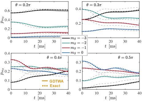
Figure 5: Benchmark of the GDTWA on a small plaquette – Time evolution of state populations for all four different initial tilt angles for the parameters used in the main text on a small $L_{x}\times L_{y}\times L_{z}=2\times 1\times 4$ plaquette. The exact-diagonalization results (points) are compared to the GDTWA predictions (lines). The GDTWA provides excellent quantitative predictions on the considered time-scale. As a comparison, the large system GDTWA ($6\times 3\times 6$) results are shown as thin dashed grey lines.

I.7 Benchmark of the GDTWA on a small plaquette

We simulate dynamics of atoms in a 3D lattice geometry. The rapid Hilbert-space growth with system size ($7^{N}$) prohibits an exact diagonalization simulation in a real 3D system. The lattice constants in the different dimensions are $(d_{x},d_{y},d_{z})\approx(1.12,2.24,1.01)\times\lambda/2$. Due to this geometry and the large spacing along the $y$-direction, dipole-couplings along the $y$ dimension are relatively small. Thus, to check the validity of our GDTWA simulation, we benchmark it against the exact solution on a small 2D plaquette in the $x-z$ plane. Fig. 5 shows a benchmark of the GDTWA prediction for the population dynamics for all different tilt angles on a $L_{x}\times L_{y}\times L_{z}=2\times 1\times 4$ plaquette (otherwise the same parameters as in the main text are used). The agreement of the GDTWA (lines) with the ED results (points) is remarkable. Furthermore, we note that modeling the experiment with larger 3D system sizes remains crucial, as is seen by the large difference to the GDTWA result for the large $6\times 3\times 6$ system.

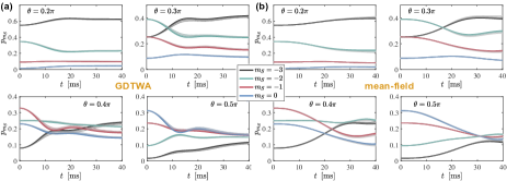
Figure 6: System size convergence: Time evolution of state populations for all four different initial tilt angles for the parameters used in the main text. The 3D system size $L_{x}\times L_{y}\times L_{z}$ is increased. (a) Results for GDTWA simualtions ($B_{Q}=4.4\,\text{Hz}$). Three lines from light to dark color are for $L_{y}=3$, and $L_{x}=L_{z}=4,5,6$. The dashed lines are for a $4\times 4\times 4$ system and the overlap of the dashed line with the $4\times 3\times 4$ demonstrates convergence in the $y$ direction. (b) Same results for mean-field simulations ($B_{Q}=1.4\,\text{Hz}$), light to dark lines are for $L_{y}=4$, and $L_{x}=L_{z}=9,11,13$, and dashed lines are for a $11\times 3\times 11$ system.

I.8 System size convergence in numerical simulations

Even with the classical equations it is very hard to model the macroscopic number of $10^{4}$ atoms in the experiment. We therefore simulate the population dynamics of a bulk of atoms by using a small 3D $L_{x}\times L_{y}\times L_{z}$ block of increasing size and checking for finite size convergence. Due to the lattice geometry (with increased spacing in the $y$ direction) finite size convergence is achieved for values $L_{y}<L_{x},L_{z}$. Our finite size comparisons are summarized in Fig. 6 for both our GDTWA and mean-field simulations. In the GDTWA case it is evident that a size of $L_{x}\times L_{y}\times L_{z}=6\times 3\times 6$ already give well converged results for all populations and all tilt angles on our time-scale of interest (for the results in the main text we use a $7\times 3\times 7$ block).

The mean-field result requires much larger system sizes for finite size convergence. This is a direct consequence of the different thermalization mechanism of the mean-field dynamics. Individual spin-density matrices remain pure in the mean-field case throughout the simulation. Finite entropy only builds up in the system-averaged local spin-density matrix, and stems from an inhomogeneous evolution of local phases due to field-gradients and finite-size effects. Therefore large system sizes are required for a converged average. In the main text, we use a system size of $L_{x}\times L_{y}\times L_{z}=13\times 4\times 13$, which provides converged results on our time-scale of interest [cf. Fig. 6(b)].

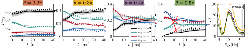
Figure 7: Identical to Fig. 2a, but instead of the best fitting $B_{Q}$ value, the best fitting positive value of $B_{Q}$ is chosen: Comparison of experimental data with GDTWA simulations of the four lowest spin-level populations, $p_{m_{S}}$, for various initial tilting angles $\theta=0.2\pi$, $0.3\pi$, $0,4\pi$, and $0.5\pi$ on a $7\times 3\times 7$ cluster allowing the quadratic Zeeman field $B_{Q}$ to be the only fitting parameter [here: $B_{Q}=6.3\text{Hz}$]. The red solid line (for $\theta=0.5\pi$) is the result of the perturbative expansion, Eq. (3). The shaded area indicates the range of variation of the populations for evolutions with $\Delta B_{Q}=\pm 0.3\,\text{Hz}$ and uncertainties in the tilting angles with $\theta=(0.2\pm 0.018\pi),(0.3\pm 0.012)\pi,(0.4\pm 0.012)\pi,(0.5\pm 0.01)\pi$ (estimated from the experiment).

I.9 Details on determination of best quadratic shift

Here, we provide more details on our determination of the best value of $B_{Q}$, which we take as only fitting parameter for the full numerical simulations to the experimental data points. We compute the deviation from each experimental data point as $\chi^{2}_{m_{S}}(t)=[p_{m_{S}}^{[\text{sim.}]}(t)-p_{m_{S}}^{[\text{exp.}]}(t)]^{2}/\sigma^{2}_{m_{S}}(t)$, with $p_{m_{S}}^{[\text{sim./exp.}]}(t)$ the simulated and experimental state population, respectively and $\sigma_{m_{S}}(t)$ the experimental error bar for the respective data point. For each tilt angle we compute the mean deviation as $\chi^{2}=\overline{\chi^{2}_{m_{S}}(t)}$, where the average is taken over all data points (in time) and the four spin-populations. This is plotted in Fig 2 of the main text. We excluded $\theta=0.2\pi$ since at this low angle there is not significant evolution of the population. We extract the overall best fitting $B_{Q}$ from the averaged $\chi^{2}$ over all tilt angles as $B_{Q}\approx-3\,\text{Hz}$. In the mean-field case, $\chi^{2}$ deviates more wildly for large $B_{Q}$. The relatively best fit for all data points is found for $B_{Q}\approx 1.1\,\text{Hz}$. The overall deviation at the best value of $B_{Q}$ is about three times smaller for the GDTWA than for the mean-field case [$\overline{\chi^{2}}_{\rm GDTWA}\approx 2.4$ and $\overline{\chi^{2}}_{\rm MF}\approx 7.3$, respectively]. Just for completeness in Fig. 7 we also show the GDTWA dynamics at the best possible positive $B_{Q}=6.3\,\text{Hz}$, the value at which the second minimum in $\chi^{2}$ is obtained (here, $\overline{\chi^{2}}_{\rm GDTWA}\approx 3.5$). Other parameters are identical to Fig 2 in the main text. Also for this positive value of $B_{Q}$ the agreement with the experiment is decent, however, some qualitative oscillations from the simulations are not perfectly reproduced by the experiment.

For the different long-time data set used for Fig 3 we perform the identical $\chi^{2}$ optimization using an average taken over all available $7$ Zeeman sub-states but for the shown $\theta=0.5\pi$ data only. For this different data set we find an optimal $\overline{\chi^{2}}_{\rm GDTWA}\approx 1.2$ for $B_{Q}=-3.6\,$Hz, compared to a classical best fit with $\overline{\chi^{2}}_{\rm MF}\approx 2.9$ for $B_{Q}=1.1\,$Hz.

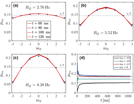
Figure 8: GDTWA vs. analytical formula: (a)-(c) Comparisons of various late time Zeeman level populations for zero magnetic field gradients and different quadratic tensor light shifts $B_{Q}=2.76\,$Hz, $B_{Q}=5.52\,$Hz, and $B_{Q}=8.28\,$Hz, respectively ($7\times 3\times 7$ lattice). The blue points show the analytical thermalization values from Eq. (6). GDTWA results converge to the thermal prediction for all the $B_{Q}$ cases displayed. (d) Long-time evolution up to $1\,$s with half the field-gradients from the experiment (and $B_{Q}=5.52\,$Hz). Horizontal dotted lines show the prediction from Eq. (6) after including the exact gradients on the $7\times 3\times 7$ block. At the experimentally relevant time-scales ($\sim 80$ms), the population redistribution stems mostly from the interactions and the quadratic tensor light shifts. Only on a much longer scale ($\sim 0.5$s) the redistribution from the field gradients causes a relaxation of the GDTWA simulation to the analytical estimation.

Figure 9: Thermalization at long time: extensive data, and comparison with our analytical model. Top 6 figures (filled circles): long time spin populations for 6 different data sets. The full lines correspond to the result of the analytical model with using $B_{Q}$ as a fitting parameter whose value is displayed in the Table. Bottom left: the empty circles correspond to average of these 6 data, the error bar corresponding to the associated standard deviation. The full line indicates 1/7. Bottom right: for each data the value of $B_{Q}$ and of the associated temperature $T$, deduced by comparing to our analytical model, are given, together with the value of the $\chi^{2}$ estimator (see above) characterizing the agreement between theory and experiment calculated over all seven spin populations.

I.10 Long-time dynamics and quantum thermalization

In the main article (see Figure 3) we discuss about the thermalization process occurring in our spin system. We derive an analytic formula which links the long time populations of the different Zeeman levels to the ones of a thermal ensemble with the same energy and magnetization of the initial state. The formula, however, is not exact. It is based on a high temperature perturbative expansion which is strictly valid in the regime $B_{Q}\ll\sqrt{V_{\rm eff}}$. In this section we benchmark the validity of the formula by comparisons with GDTWA dynamics at different quadratic fields. The summary is presented in Fig. 8(a)-(c), where we show that the analytic formula is valid for the experimental range of $B_{Q}$ parameters.

In addition to the quadratic Zeeman field, magnetic field gradients are also present in the experiment. While those terms can affect the thermalization dynamics leading to the development of spatial magnetization textures at equilibrium, we argue in the main text that such a texture is expected to occur at extremely long times in a dipolar interacting system since it requires interactions between remote parts of the cloud. Here we validate such claim using GDTWA simulations. As seen in Fig. 8(d) for the times scales currently accessible in experiments the gradients just marginally flatten out the population distribution compared to the zero gradient case.

With this validation of the analytic formula, we can use it to further characterize the asymptotic state obtained under different experimental measurements. In Fig. 9, we show all available long time data for the spin populations. As the quadratic light shift $B_{Q}$ is very sensitive to the relative intensity of the five different lattice laser beams, we expect variations of $B_{Q}$ between different data sets and therefore, accordingly to the analytic formula, a correspondent variation on the fractional populations $p_{m_{S}}$ at long times except from $p_{\pm 2}$ which should remain close to $1/7$. All these features are indeed observed in Fig. 9.

We use the model to find the $B_{Q}$ that best fits the data, and deduce from it the temperature $T$ at which thermalization takes place (see Table in Fig. 9). We point out that, similar to the case shown in Fig 2, comparing our data to the analytical model typically leads to two possible values of $B_{Q}$ (one positive, and one negative), for which the $\chi^{2}$ shows a local minimum. Distinguishing between these two local minima is difficult (i.e. they share a similar $\chi^{2}$) which is a consequence that $|B_{Q}|>|\bar{V}|$.

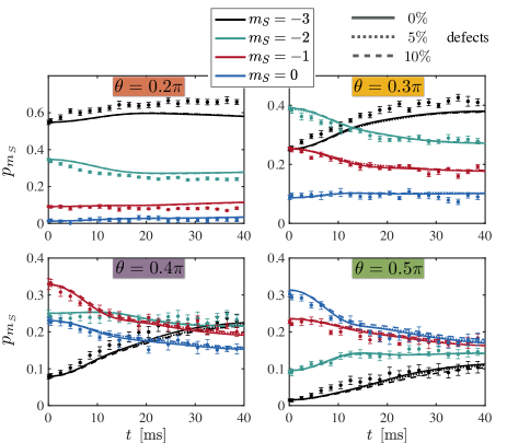
Figure 10: The effect of defects is very small. GDTWA simulations for the populations with identical parameters as in Fig. 2 of the main manuscript. Additionally, dotted and dashed lines show results for $5\%$ and $10\%$ defect density, respectively. The statistical average over $192$ different defect realizations has been taken into account. Differences are more pronounced for larger tilting angles, but still minor.

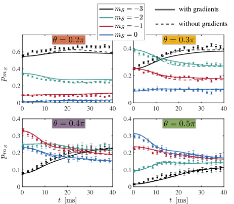
Figure 11: The effect of the magnetic field gradient is to slightly inhibit dynamics, after $\sim 10\,\text{ms}$. GDTWA simulations for the populations with identical parameters as in Fig. 2 of the main manuscript. Dashed lines show results for zero field gradient. The solid line is the usual result with the measured field gradient of $30\,\text{MHz/m}$ along the vertical axis.

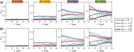
Figure 12: Comparison between classical and quantum dynamics for upper spin levels. Same panels as in Fig. 2 of the main manuscript, but for the spin levels $m=0,+1,+2,+3$.

I.11 Effect of none ideal preparation

The effect of defects due to imperfect preparation is very small. The presence of $10\%$ hole defects barely modifies the dynamics. See Fig 10.

I.12 Effect of magnetic field gradients

We also investigated the effect of magnetic field gradients. This effect is very small at short times (as expected from perturbation theory, see Eq. (3) of the main text), and only slightly inhibits dynamics at longer times, as shown in Fig.11

I.13 Dynamics of upper Zeeman sublevels not shown in main text

These are shown in Fig. 12. They were omitted in the main text to make the figure less crowded.

References

- (1) D’Alessio, L., Kafri, Y., Polkovnikov, A. and Rigol, M. From Quantum Chaos and Eigenstate Thermalization to Statistical Mechanics and Thermodynamics. Adv. Phys. 65, 239 (2016).
- (2) J. Eisert, M. Friesdorf and C. Gogolin, Quantum many-body systems out of equilibrium. Nature Physics 11, 124 (2015)
- (3) A. Kaufman et al, Quantum thermalization through entanglement in an isolated many-body system, Science 353, 794(2016)
- (4) J. G. Bohnet, et al, Quantum spin dynamics and entanglement generation with hundreds of trapped ions, Science 352, 1297 (2016)
- (5) M. Gärttner et al, Measuring out-of-time-order correlations and multiple quantum spectra in a trapped ion quantum magnet, Nature Physics 13, 781 (2017)
- (6) P. Richerme et al, Non-local propagation of correlations in long-range interacting quantum systems, Nature 511, 198 (2014)
- (7) P. Jurcevic et al, Observation of entanglement propagation in a quantum many-body system, Nature 511, 202 (2014)
- (8) P. Jurcevic et al, Direct Observation of Dynamical Quantum Phase Transitions in an Interacting Many-Body System, Phys. Rev. Lett. 119, 080501 (2017)
- (9) P. W. Hess et al, Non-thermalization in trapped atomic ion spin chains, Phil. Trans. R. Soc. A 375,0107 (2017)
- (10) J. Zeiher et al., Coherent Many-Body Spin Dynamics in a Long-Range Interacting Ising Chain, Phys. Rev. X 7, 041063 (2017)
- (11) H. Labuhn et al., Tunable two-dimensional arrays of single Rydberg atoms for realizing quantum Ising models, Nature 534, 667 (2016)
- (12) H. Bernien et al,Probing many-body dynamics on a 51-atom quantum simulator, Nature 551, 579 (2017)
- (13) B. Yan et al, Observation of dipolar spin-exchange interactions with lattice-confined polar molecules, Nature 501, 521 (2013)
- (14) K. R. A. Hazzard et al, Many-Body Dynamics of Dipolar Molecules in an Optical Lattice. Phys. Rev. Lett. 113, 195302 (2014)
- (15) A. de Paz et al, Nonequilibrium Quantum Magnetism in a Dipolar Lattice Gas, Phys. Rev. Lett. 111, 185305 (2013)
- (16) A. de Paz, et al, Probing spin dynamics from the Mott insulating to the superfluid regime in a dipolar lattice gas, Phys. Rev. A 93, 021603(R) (2016)
- (17) J. Schachenmayer, A. Pikovski, and A. M. Rey., Many-Body Quantum Spin Dynamics with Monte Carlo Trajectories on a Discrete Phase Space, Phys. Rev. X 5, 011022 (2015).
- (18) J. Schachenmayer, A. Pikovski, and A. M. Rey., Dynamics of correlations in two-dimensional quantum spin models with long-range interactions: a phase-space Monte-Carlo study, New J.Phys. 17, 065009 (2015).
- (19) A. Polkovnikov, Phase space representation of quantum dynamics, Ann. Phys. 325, 1790 (2010)
- (20) P.A. Lee, N. Nagaosa and X.G. Wen, Rev. Mod. Phys. 78, 17 (2006)
- (21) R. Blatt and C.F. Roos, Nature Physics 8, 277 (2012)
- (22) M. Saffman, T.G. Walker and K. Mølmer, Rev. Mod. Phys. 82, 2313 (2010)
- (23) A. Renyi. Proceedings of the Fourth Berkeley Symposium on Mathematics: Statistics and Probability, 1, 547 (1960).
- (24) J.L. Bohn, A.M. Rey and J. Ye, Cold molecules: Progress in quantum engineering of chemistry and quantum matter, Science 357, 6355 (2017)
- (25) T. Lahaye and C. Menotti and L. Santos and M. Lewenstein and T. Pfau, The physics of dipolar bosonic quantum gases, Rep. Prog. Phys.72, 126401 (2009)
- (26) D. Aharonov, D. Gottesman, S. Irani, and J. Kempe, in Foundations of Computer Science, 48th Annual IEEE Symposium, FOCS 07, 373 (2007)
- (27) S. Hallgren, D. Nagaj, and S. Narayanaswami, The Local Hamiltonian Problem on a Line with Eight States is QMAComplete, Quantum Inf. Comput. 13, 0721 (2013)
- (28) S. Lepoutre, et al, Spin mixing and protection of ferromagnetism in a spinor dipolar condensate, Phys. Rev. A 97, 023610 (2018)
- (29) B. Pasquiou et al, Control of dipolar relaxation in external fields, Phys. Rev. A 81, 042716 (2010)
- (30) K. R. A. Hazzard, S. R. Manmana, M. Foss-Feig, and A. M. Rey, Far-from-Equilibrium Quantum Magnetism with Ultracold Polar Molecules, Phys. Rev. Lett. 110, 075301 (2013)
- (31) A. Abragam, Principles of Nuclear Magnetism, Clarendon, Oxford, UK (1983)
- (32) K. R. A. Hazzard et al. Quantum correlations and entanglement in far-from-equilibrium spin systems, Phys. Rev. A 90, 063622(2014)
- (33) R.A. Bertlmann and P. Krammer, Bloch vectors for qudits, J. Phys. A: Math. Theor. 41, 235303 (2008)
- (34) A. Piñeiro Orioli et al, Relaxation of an isolated dipolar-interacting Rydberg quantum spin system. Phys. Rev. Lett. 120, 063601 (2018)
- (35) Y. Tang, W. Kao, K.Y. Li, S. Seo, K. Mallayya, M. Rigol, S. Gopalakrishnan and B.L. Lev, Phys. Rev. X 8, 021030 (2018)
- (36) T. Kinoshita, T. Wenger and D. S. Weiss, Nature 440, 900 (2018)
- (37) T. Langen, S. Erne, R. Geiger, B. Rauer, T. Schweigler, M. Kuhnert, W. Rohringer, I.E. Mazets, T. Gasenzer, and J. Schmiedmayer, Science 348, 207 2015