Frequency-dependent Alfvén-wave propagation in the solar wind:
Onset and suppression of parametric decay instability

Abstract

Using numerical simulations we investigate the onset and suppression of parametric decay instability (PDI) in the solar wind, focusing on the suppression effect by the wind acceleration and expansion. Wave propagation and dissipation from the coronal base to $1{\rm\ au}$ is solved numerically in a self-consistent manner; we take into account the feedback of wave energy and pressure in the background. Monochromatic waves with various injection frequencies $f_{0}$ are injected to discuss the suppression of PDI, while broadband waves are applied to compare the numerical results with observation. We find that high-frequency ($f_{0}\gtrsim 10^{-3}{\rm\ Hz}$) Alfvén waves are subject to PDI. Meanwhile, the maximum growth rate of the PDI of low-frequency ($f_{0}\lesssim 10^{-4}{\rm\ Hz}$) Alfvén waves becomes negative due to acceleration and expansion effects. Medium-frequency ($f_{0}\approx 10^{-3.5}{\rm\ Hz}$) Alfvén waves have a positive growth rate but do not show the signature of PDI up to 1 au because the growth rate is too small. The medium-frequency waves experience neither PDI nor reflection so they propagate through the solar wind most efficiently. The solar wind is shown to possess frequency-filtering mechanism with respect to Alfvén waves. The simulations with broadband waves indicate that the observed trend of the density fluctuation is well explained by the evolution of PDI while the observed cross-helicity evolution is in agreement with low-frequency wave propagation.

1 Introduction

It is widely accepted that Alfvén waves (Alfvén, 1942) play an important role in the heating (Alfvén, 1947; Osterbrock, 1961; Matthaeus et al., 1999) and acceleration (Belcher, 1971; Jacques, 1977; Heinemann & Olbert, 1980) of the solar wind. Indeed, Alfvén waves are observed in the solar atmosphere (De Pontieu et al., 2007; Tomczyk et al., 2007; McIntosh et al., 2011; Srivastava et al., 2017) and solar wind (Coleman, 1968; Belcher & Davis, 1971). Nonthermal line width (Banerjee et al., 2009; Hahn & Savin, 2013) and Faraday-rotation fluctuations (Hollweg et al., 1982, 2010) also indicate the existence of Alfvén waves in the corona. Meanwhile, the dissipation process of Alfvén waves in the corona and solar wind is still under discussion. Since the amount and location of Alfvén-wave dissipation vary with respect to the mechanism and strongly affect the coronal temperature and wind velocity (Hansteen & Velli, 2012), clarifying the elemental processes is important not only for plasma physics but also for space weather.

There are several processes of Alfvén-wave dissipation. If there are counter-propagating Alfvén waves, Alfvén-wave turbulence (Iroshnikov, 1964; Kraichnan, 1965; Dobrowolny et al., 1980; Goldreich & Sridhar, 1995) evolves. In the corona and solar wind, because of the inhomogeneity, Alfvén waves partially reflect (Ferraro & Plumpton, 1958; Heinemann & Olbert, 1980; An et al., 1990; Velli, 1993; Cranmer & van Ballegooijen, 2005) and Alfvén-wave turbulence is sustained (Dmitruk & Matthaeus, 2003; Oughton et al., 2006). This reflection-driven Alfvén-wave turbulence is frequently studied (Matthaeus et al., 1999; Dmitruk et al., 2002; Verdini & Velli, 2007; Perez & Chandran, 2013; van Ballegooijen & Asgari-Targhi, 2016), and some models explain the heating and acceleration of the solar wind self-consistently (Cranmer et al., 2007; Verdini et al., 2010). Alfvén-wave turbulence is also important for the energy cascade and the formation of the power spectrum (Verdini et al., 2012; van Ballegooijen & Asgari-Targhi, 2017).

When the Alfvén velocity is inhomogeneous perpendicular to the magnetic field lines, phase mixing begins (Heyvaerts & Priest, 1983; De Groof & Goossens, 2002; Goossens et al., 2012). The density variation across the magnetic field lines is observed in the corona (Tian et al., 2011; Raymond et al., 2014), and this indicates the possibility of phase mixing. Several studies show the role of phase mixing and related phenomena in the solar atmosphere (Antolin et al., 2015; Kaneko et al., 2015). Recently, it was numerically shown that phase mixing can generate turbulent structure (Magyar et al., 2017).

Since the amplitude of an Alfvén wave is not small and the plasma beta is low (Gary, 2001; Iwai et al., 2014; Bourdin, 2017), the (extended) corona and solar wind are preferable locations for the development of parametric decay instability (PDI). PDI is a type of instability of an Alfvén wave (Galeev & Oraevskii, 1963; Sagdeev & Galeev, 1969; Goldstein, 1978; Derby, 1978) and was recently observed in laboratory plasma (Dorfman & Carter, 2016) and in the solar wind (Bowen et al., 2018). As a result of PDI, a large-amplitude longitudinal wave is generated (Hoshino & Goldstein, 1989; Del Zanna et al., 2001), and the plasma is heated up by the resultant shock wave. Suzuki & Inutsuka (2005, 2006) demonstrated that, without Alfvén-wave turbulence, the coronal heating and solar-wind acceleration are explained self-consistently by PDI. These studies were extended to two dimensions (2D) by Matsumoto & Suzuki (2012, 2014). In addition, the cross-helicity evolution in the fast solar wind (Bavassano et al., 1982, 2000) might be due to PDI (Malara & Velli, 1996; Malara et al., 2000; Shoda & Yokoyama, 2016). Chandran (2018) also argued that the $1/f$ spectrum observed in the fast solar wind (Bruno & Carbone, 2013) possibly results from PDI.

We note that Alfvén-wave turbulence and PDI are not independent of each other, because PDI generates large-amplitude backscattered Alfvén waves (Sagdeev & Galeev, 1969; Goldstein, 1978) and enhances the heating by Alfvén-wave turbulence. Shoda et al. (2018) showed that, due to PDI, the turbulence heating rate per unit mass increases ($\sim 10^{11}{\rm\ erg\ g^{-1}\ s^{-1}}$) compared with the reduced- magnetohydrodynamic MHD (without-PDI) value ($\sim 10^{10}{\rm\ erg\ g^{-1}\ s^{-1}}$) (Perez & Chandran, 2013; van Ballegooijen & Asgari-Targhi, 2016).

Amongst the aforementioned dissipation processes, we focus on PDI in this study. The PDI of monochromatic Alfvén waves in a time-independent, uniform background with MHD approximation is well studied. In the limit of $\beta\ll 1$ and $\eta=\delta B/B_{0}\ll 1$ where $B_{0}$ and $\delta B$ denote the mean and fluctuating magnetic field, respectively, the growth rate is given as (Galeev & Oraevskii, 1963; Sagdeev & Galeev, 1969)

$$\gamma/\omega_{0}=\frac{1}{2}\eta\beta^{-1/4},$$ (1)

where $\omega_{0}$ is the angular frequency of the parent wave. Here we define $\beta$ as

$$\beta=c_{s}^{2}/v_{A}^{2},$$ (2)

where $c_{s}$ and $v_{A}$ denote the sound and Alfvén speed, respectively. The general dispersion relation that considers full four-wave interaction (Lashmore-Davies, 1976) is given by Goldstein (1978) and Derby (1978) as

$$\left(\omega-k\right)\left(\omega^{2}-\beta k^{2}\right)\left[\left(\omega+k\right)^{2}-4\right]$$

$$=\eta^{2}k^{2}\left(\omega^{3}+k\omega^{2}-3\omega+k\right),$$ (3)

where $\omega$ and $k$ are normalized by the parent-wave frequency $\omega_{0}$ and wavenumber $k_{0}$. In this study, we call Eq. (3) the Goldstein–Derby dispersion relation. By solving Eq. (3), Goldstein (1978) confirmed that the classical understanding that the parent wave decays into a forward acoustic wave and a backward Alfvén wave is correct in the low-beta regime. In the high-beta plasma, however, the behavior of the instability changes (Jayanti & Hollweg, 1993). The linear stage of this ideal (monochromatic, time-independent, and uniform) case is well understood. The nonlinear stage of PDI is also frequently studied using numerical simulation. Hoshino & Goldstein (1989) studied the linear-to-nonlinear evolution of PDI. This study was extended to multi-dimensional simulations in both low- and high-beta cases (Ghosh & Goldstein, 1994; Ghosh et al., 1994). Del Zanna et al. (2001) investigated the evolution of PDI with different plasma parameters, different dimensions and different boundary conditions to show the robustness of PDI. Recently, the three-dimensional (3D) hybrid simulation of PDI-driven turbulence has been studied (Fu et al., 2017).

There are several studies on the linear growth rate of PDI under non-ideal situations. Two-fluid and kinetic simulations were performed (Terasawa et al., 1986; Nariyuki et al., 2008) The PDI of non-monochromatic Alfvén waves tends to have a smaller growth rate (Cohen & Dewar, 1974; Umeki & Terasawa, 1992; Malara & Velli, 1996; Malara et al., 2000). If the background is turbulent, the growth rate is quenched compared with the ideal value (Shi et al., 2017). The solar wind acceleration and expansion also work to reduce the growth rate (Tenerani & Velli, 2013; Del Zanna et al., 2015). Recently the effect of temperature anisotropy on PDI has also been also studied (Tenerani et al., 2017).

Specifically in the solar wind close to the Sun, wind acceleration and expansion play an important role. Such effects are frequently studied using a local co-moving box in the so-called accelerating expanding box (AEB) model (Velli et al., 1992; Grappin et al., 1993; Grappin & Velli, 1996; Tenerani & Velli, 2017). One problem with the AEB model is that the dynamics and energetics are not self-consistent; initially, we have to assume the background quantities such as flow speed or Alfvén speed and ignore the feedback of wave heating and acceleration on them. Our motivation is to test the idea obtained from the AEB model using a non-local simulation box that extends from the corona to the distant heliosphere.

This paper is organized as follows. In Section 2, we describe the basic equations, numerical scheme, and boundary conditions used in this study. Section 3 and Section 4 describe the results with monochromatic wave injection and broadband wave injection, respectively. We summarize this paper in Section 5

2 Numerical method

2.1 Basic equations and setting

We used the same equations as those in Shoda et al. (2018) and considered a one-dimensional system whose coordinate $r$ is curved along the background magnetic field line. The basic equations used were

$$\frac{\partial}{\partial t}\left(\rho r^{2}f\right)+\frac{\partial}{\partial r}\left(\rho v_{r}r^{2}f\right)=0,$$ (4)

$$\frac{\partial}{\partial t}\left(\rho v_{r}r^{2}f\right)+\frac{\partial}{\partial r}\left[\left(\rho{v_{r}}^{2}+p+\frac{{\mbox{\boldmath$B$}_{\perp}}^{2}}{8\pi}\right)r^{2}f\right]$$

$$=\left(p+\frac{\rho{\mbox{\boldmath$v$}_{\perp}}^{2}}{2}\right)\frac{d}{dr}\left(r^{2}f\right)-\rho gr^{2}f,$$ (5)

$$\frac{\partial}{\partial t}\left(\rho\mbox{\boldmath$v$}_{\perp}r^{3}f^{3/2}\right)+\frac{\partial}{\partial r}\left[\left(\rho v_{r}\mbox{\boldmath$v$}_{\perp}-\frac{B_{r}\mbox{\boldmath$B$}_{\perp}}{4\pi}\right)r^{3}f^{3/2}\right]$$

$$=-\hat{\mbox{\boldmath$\eta$}}_{1}\cdot\rho\mbox{\boldmath$v$}_{\perp}r^{3}f^{3/2}-\hat{\mbox{\boldmath$\eta$}}_{2}\cdot\sqrt{\frac{\rho}{4\pi}}\mbox{\boldmath$B$}_{\perp}r^{3}f^{3/2},$$ (6)

$$\frac{\partial}{\partial t}\left(\mbox{\boldmath$B$}_{\perp}r\sqrt{f}\right)+\frac{\partial}{\partial r}\left[\left(\mbox{\boldmath$B$}_{\perp}v_{r}-B_{r}\mbox{\boldmath$v$}_{\perp}\right)r\sqrt{f}\right]$$

$$=-\hat{\mbox{\boldmath$\eta$}}_{1}\cdot\mbox{\boldmath$B$}_{\perp}r\sqrt{f}-\hat{\mbox{\boldmath$\eta$}}_{2}\cdot\sqrt{4\pi\rho}\mbox{\boldmath$v$}_{\perp}r\sqrt{f},$$ (7)

$$\frac{d}{dr}\left(B_{r}r^{2}f\right)=0,$$ (8)

$$\frac{\partial}{\partial t}\left[\left(e+\frac{1}{2}\rho\mbox{\boldmath$v$}^{2}+\frac{\mbox{\boldmath$B$}^{2}}{8\pi}\right)r^{2}f\right]$$

$$+\frac{\partial}{\partial r}\left[\left(e+p+\frac{1}{2}\rho\mbox{\boldmath$v$}^{2}+\frac{{\mbox{\boldmath$B$}_{\perp}}^{2}}{4\pi}\right)v_{r}r^{2}f-B_{r}\frac{\mbox{\boldmath$B$}_{\perp}\cdot\mbox{\boldmath$v$}_{\perp}}{4\pi}r^{2}f\right]$$

$$=r^{2}f\left(-\rho gv_{r}+Q_{\rm cond}\right),$$ (9)

$$e=\frac{p}{\Gamma-1},\ \ \ \ p=\frac{\rho k_{B}T}{\mu}.\$$ (10)

See Appendix in Shoda & Yokoyama (2018) for the derivation. We denoted the perpendicular components of $X$ as $\mbox{\boldmath$X$}_{\perp}=X_{x}\mbox{\boldmath$e$}_{x}+X_{y}\mbox{\boldmath$e$}_{y}$, and we assumed that the plasma is composed of only hydrogen and is fully ionized in the entire simulation region. Therefore, the mean molecular mass $\mu$ satisfied $\mu=0.5m_{p}$ where $m_{p}$ is the proton mass. $\Gamma$ is the adiabatic specific heat: $\Gamma=5/3$.

$f$ is the expansion factor of the flux tube (Levine et al., 1977; Wang & Sheeley, 1990; Arge & Pizzo, 2000). In this study, following Kopp & Holzer (1976) and Verdini et al. (2010), we assumed

$$f(r)=\frac{f_{\rm exp}\exp\left[\left(r-r_{f}\right)/\sigma\right]+f_{1}}{\exp\left[\left(r-r_{f}\right)/\sigma\right]+f_{1}},$$ (11)

where $f_{1}=1-f_{\rm exp}\exp\left[\left(R_{\odot}-r_{f}\right)/\sigma\right]$, $f_{\rm exp}=10$, $r_{f}=1.3R_{\odot}$ and $\sigma=0.5R_{\odot}$.

$\hat{\mbox{\boldmath$\eta$}}_{1}$ and $\hat{\mbox{\boldmath$\eta$}}_{2}$ are coefficient tensors that represent phenomenological turbulent decay.

$$\hat{\mbox{\boldmath$\eta$}}_{1}=\frac{c_{d}}{4\lambda}\left(\begin{array}[]{cc}|z^{+}_{x}|+|z^{-}_{x}|&0\\ 0&|z^{+}_{y}|+|z^{-}_{y}|\\ \end{array}\right),$$ (14)

$$\hat{\mbox{\boldmath$\eta$}}_{2}=\frac{c_{d}}{4\lambda}\left(\begin{array}[]{cc}|z^{+}_{x}|-|z^{-}_{x}|&0\\ 0&|z^{+}_{y}|-|z^{-}_{y}|\\ \end{array}\right),$$ (17)

where $z^{\pm}_{x,y}$ are Elsässer variables (Elsässer, 1950):

$$z^{\pm}_{x,y}=v_{x,y}\mp B_{x,y}/\sqrt{4\pi\rho}.$$ (18)

Shoda et al. (2018) showed that these terms are a natural extension of a widely used phenomenological model of Alfvén-wave turbulence (Hossain et al., 1995; Dmitruk et al., 2002; Verdini & Velli, 2007; Chandran & Hollweg, 2009). $c_{d}=0.1$ was chosen in this study (van Ballegooijen & Asgari-Targhi, 2017). $\lambda$ is the perpendicular correlation length of turbulence. We assumed that the correlation length is proportional to the flux-tube radius:

$$\lambda\propto B_{r}^{-1/2}.$$ (19)

Using the phenomenological turbulence term together with Eq. (19), both local (Cranmer et al., 2007; Verdini et al., 2010; Lionello et al., 2014; Shoda et al., 2018) and global (van der Holst et al., 2014) simulations succeeded in modeling the corona and solar wind. The correlation length at the coronal base ($\lambda_{0}$) is

$$\lambda_{0}=1{\rm\ Mm}.$$ (20)

This is based on the assumption that Alfvén waves are generated inside the magnetic patches on the photosphere and propagate upward along the flux tube (van Ballegooijen et al., 2011).

$Q_{\rm cond}$ is the heating by thermal conduction given as

$$Q_{\rm cond}=-\nabla\cdot\mbox{\boldmath$q$}_{\rm cond}=-\frac{1}{r^{2}f}\frac{\partial}{\partial r}\left(r^{2}fq_{\rm cond}\right),$$ (21)

where $\mbox{\boldmath$q$}_{\rm cond}$ is the conductive flux and $q_{\rm cond}$ represents its radial component. The conductive flux is a combination of Spitzer-Härm flux (Spitzer & Härm, 1953) and free-streaming flux (Hollweg, 1974, 1976) given as

$$q_{\rm cond}=\xi q_{\rm SH}+(1-\xi)q_{\rm FS},\ \ \ \ \xi=\max\left(1,\frac{\rho}{\rho_{\rm SW}}\right)$$ (22)

where $\rho_{\rm SW}=10^{-21}{\rm g\ cm^{-3}}$ and

$$q_{\rm SH}=-\kappa_{0}T^{5/2}\frac{\partial}{\partial r}T,$$ (23)

$$q_{\rm FS}=\frac{3}{4}\alpha pv_{r}.$$ (24)

In GGS-Gaussian units, $\kappa_{0}\approx 10^{-6}$. We fixed $\alpha=2$ in this study.

Radiative cooling is ignored because of its small contribution to the coronal energy budget (Matsumoto & Suzuki, 2014; van Ballegooijen & Asgari-Targhi, 2016). The coronal base is cooled down by keeping the bottom temperature fixed.

2.2 Numerical scheme and boundary conditions

We solved the basic equations (4)-(10) from the coronal base ($r=1.014R_{\odot}$) to 1 au ($r=215R_{\odot}$). Furthermore, we applied 50 000 uniform grid points to resolve the computational domain. The Harten-Lax-van Leer-discontinuities (HLLD) approximated Riemann solver (Miyoshi & Kusano, 2005) with 2nd-order monotone upstream-centered schemes for conservation law (MUSCL) reconstruction (van Leer, 1979) was used to calculate the numerical flux, while the 3rd-order strong stability preserving (SSP) Runge-Kutta method (Shu & Osher, 1988) was used for time integration.

The free boundary condition was imposed on the boundary at 1 au. We confirmed that the boundary condition at 1 au does not affect the calculation because the super-sonic and super-Alfvénic solar wind is formed in a quasi-steady state. This is why we did not need to apply the transmitting boundary condition (Thompson, 1987; Del Zanna et al., 2001; Suzuki & Inutsuka, 2006). As for the lower boundary, the conditions were as follows. Here we denoted the lower-boundary values with subscript $0$. The mass density $\rho$, temperature $T$, and radial magnetic field strength $B_{r}$ were fixed to

$$\rho_{0}=8.5\times 10^{-16}{\rm\ g\ cm^{-3}},\ \ T_{0}=4\times 10^{5}{\rm\ K},\ \ B_{r,0}=10{\rm\ G}.$$ (25)

The quantity $B_{r,0}/f_{\rm exp}$ controls the solar-wind velocity (Suzuki, 2004, 2006; Fujiki et al., 2015; Réville & Brun, 2017). According to Fujiki et al. (2015), our setting of ($B_{r,0}/f_{\rm exp}=1{\rm\ G}$) approximately corresponds to $650{\rm\ km\ s^{-1}}$ in terms of asymptotic solar wind velocity.

We applied the free boundary conditions for the radial velocity and inward Elsässer variable:

$$\left.\frac{\partial}{\partial r}v_{r}\right|_{0}=0,\ \ \ \ \left.\frac{\partial}{\partial r}\mbox{\boldmath$z$}^{-}\right|_{0}=0,$$ (26)

where $\mbox{\boldmath$z$}^{-}=\mbox{\boldmath$v$}_{\perp}+\mbox{\boldmath$B$}_{\perp}/\sqrt{4\pi\rho}$. As for the upward Elsässer variable, $\mbox{\boldmath$z$}^{+}=\mbox{\boldmath$v$}_{\perp}-\mbox{\boldmath$B$}_{\perp}/\sqrt{4\pi\rho}$, we applied monochromatic (Section 3) or broadband (Section 4) wave injections. In both cases, the root-mean-square value of the transverse velocity $v_{\rm rms,0}$ was fixed to $v_{\rm rms,0}=32{\rm\ km\ s^{-1}}$. In terms of the upward Elsässer variable, the root-mean-square value was $z^{+}_{\rm rms,0}=2v_{\rm rms,0}$, because $\left|z^{+}_{x,y}\right|\gg\left|z^{-}_{x,y}\right|$ at the coronal base and

$$z^{+}_{\rm rms,0} =\sqrt{{z^{+}_{x}}^{2}+{z^{+}_{y}}^{2}}$$

$$\simeq\sqrt{\left(z^{+}_{x}+z^{-}_{x}\right)^{2}+\left(z^{+}_{y}+z^{-}_{y}\right)^{2}}$$

$$=\sqrt{4\left(v_{x}^{2}+v_{y}^{2}\right)}=2v_{\rm rms,0}.$$ (27)

Note that the injected energy flux $F_{0}$ was kept constant:

$$F_{0}=\frac{1}{4}\rho{z^{+}_{0}}^{2}v_{A,0}=8.4\times 10^{5}{\rm\ erg\ cm^{-3}\ s^{-1}}.$$ (28)

This was larger than the required amount of energy injection required to sustain the solar wind in the open field regions (Withbroe & Noyes, 1977).

3 Monochromatic-wave injection

We first applied the monochromatic wave injections with different frequencies to discuss the basic properties. The boundary condition of the upward Elsässer variable was

$$z^{+}_{x,0}=2v_{\rm rms,0}\sin\left(2\pi f_{0}t\right),$$ (29)

$$z^{+}_{y,0}=2v_{\rm rms,0}\cos\left(2\pi f_{0}t\right),$$ (30)

where $f_{0}$ is the injection frequency.

3.1 Quasi-steady state

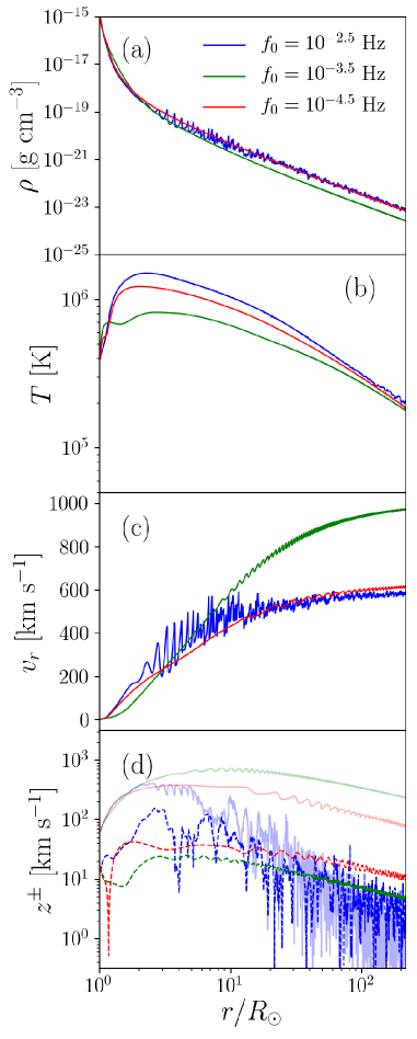
Figure 1: Snapshots of the quasi-steady states with different wave-injection frequencies. Blue, green and red lines indicate $f_{0}=10^{-2.5}{\rm\ Hz}$, $10^{-3.5}{\rm\ Hz}$, $10^{-4.5}{\rm\ Hz}$, respectively. Panels correspond to a: mass density, b: temperature, c: radial velocity, d: Elsässer variables. In Panel d, transparent and dashed lines indicate $z^{+}$ and $z^{-}$, respectively.

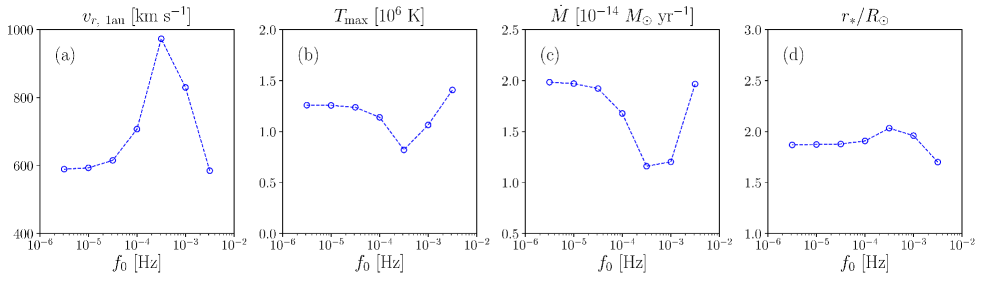
Figure 2: Parameters of the corona and solar wind as functions of wave-driving frequency. Panels indicate the a: solar wind speed at 1 au, b: maximum coronal temperature, c: mass-loss rate, and d: sonic point location. Each parameter is measured in the time-averaged quasi-steady states.

Figure 1 shows the snapshots of the quasi-steady states of different injection frequencies: $f_{0}=10^{-2.5}{\rm\ Hz\ (blue)}$, $10^{-3.5}{\rm\ Hz\ (green)}$, $10^{-4.5}{\rm\ Hz\ (red)}$. Panels indicate from top to bottom the mass density $\rho$, temperature $T$, radial velocity $v_{r}$, and Elsässer variables $z^{\pm}=\sqrt{{z_{x}^{\pm}}^{2}+{z_{y}^{\pm}}^{2}}$ (transparent: $z^{+}$, dashed: $z^{-}$).

Although the same amount of energy flux ($F_{0}=8.4\times 10^{5}{\rm\ erg\ cm^{-3}\ s^{-1}}$) was injected in each case, the corresponding quasi-steady states showed different properties. Firstly, a significant density fluctuation is observed when $f_{0}=10^{-2.5}{\rm\ Hz}$. Because the large density fluctuation is attributed to PDI, it indicates that PDI can develop only when $f_{0}>10^{-3.5}{\rm\ Hz}$. Elsässer variables also show evidence of PDI when $f_{0}=10^{-2.5}{\rm\ Hz}$. The ratio $z^{+}/z^{-}$ is smaller than unity partly in $r/R_{\odot}>50$ when $f_{0}=10^{-2.5}{\rm\ Hz}$, while $z^{+}/z^{-}\gg 1$ when $f_{0}\lesssim 10^{-3.5}{\rm\ Hz}$. A natural interpretation of low $z^{+}/z^{-}$ is that, as a result of PDI, a large amount of reflected Alfvén waves is generated (Sagdeev & Galeev, 1969; Goldstein, 1978; Suzuki & Inutsuka, 2005) and is advected to 1 au. The coronal temperature is the lowest in the medium-frequency case ($f_{0}=10^{-3.5}{\rm\ Hz}$). When $f_{0}$ is high, because PDI occurs in the sub-Alfvénic corona, the coronal plasma is heated up by the shock and turbulence driven by PDI (Shoda et al., 2018). However, when $f_{0}$ is low, Alfvén waves reflect efficiently (An et al., 1990; Velli, 1993; Cranmer & van Ballegooijen, 2005) and the turbulence heating in the corona increases (Matthaeus et al., 1999; Dmitruk et al., 2002; Oughton et al., 2006). This is why the medium-frequency case, in which PDI does not occur and reflection is weak, shows the lowest temperature of the corona. As a result of the lower-temperature corona, the mass density of the wind is smaller and the wind is faster (Hansteen & Velli, 2012).

In Figure 2, we show the dependence of solar wind parameters on $f_{0}$. From left to right, we show the solar-wind velocity $v_{r}$ at $r=1{\rm\ au}$, maximum temperature $T_{\rm max}$, mass-loss rate $\dot{M}=\rho v_{r}4\pi r^{2}$, and the sonic point $r_{\ast}$ where the sound speed $c_{s}$ is equal to the wind speed $v_{r}$. Here, we assumed $c_{s}=\sqrt{p/\rho}$ because the plasma is almost isothermal due to the strong thermal conduction near the sonic point. Every variable is averaged in time over $10^{5}{\rm\ s}$.

Figure 2 shows that the solar wind properties depend non-monotonically on $f_{0}$; slow, high-temperature, and high-density winds are driven in the cases with high and low $f_{0}$; in contrast, fast, low-temperature, and low-density winds stream out in the cases with intermediate $f_{0}$. As explained before, this bimodal behavior can be understood by the different characters of the reflection and dissipation of low- and high-frequency Alfvén waves; low-frequency waves dissipate by reflection-driven turbulence and high-frequency waves by PDI. In addition, Fig. 2 indicates that the corona and solar wind have a frequency-filtering mechanism; waves with a medium frequency $f_{0}\sim 10^{-3.5}{\rm\ Hz}$ are the least dissipative and most transparent in order to propagate through. This might be responsible for the dominance of the hour-scale Alfvén waves observed in the solar wind (Belcher & Davis, 1971).

Some features found in Fig. 2 are consistent with previous research. In the high-frequency range, the solar wind velocity (Fig. 2a) decreases as $f_{0}$ increases, and this result is consistent with Ofman & Davila (1998), who showed the inverse correlation between the injection frequency and the resultant wind speed when $0.35{\rm\ mHz}\lesssim f_{0}\lesssim 3{\rm\ mHz}$. The critical point $r_{*}$ (Fig. 2d) has a negative correlation with the temperature. This is because the critical point is closer to the Sun when the sound speed is larger (Parker, 1958).

3.2 Decay law of density fluctuation in the accelerating and expanding solar wind

Following Tenerani & Velli (2013), we derived the linear decay law for slow magnetoacoustic waves in the accelerating and expanding solar wind. We began with the conservation of mass: Eq. (4). Assuming that the density and radial velocity have mean $\rho_{0}$, $v_{r,0}$ and small fluctuation $\delta\rho$, $\delta v_{r}$ parts, we could express the linearized equation for $\delta\rho$ as

$$\frac{\partial}{\partial t}\left(\delta\rho S\right)+\frac{\partial}{\partial r}\left(\rho_{0}\delta v_{r}S\right)+\frac{\partial}{\partial r}\left(\delta\rho v_{r,0}S\right)=0.$$ (31)

where $S=r^{2}f$ represents the cross section of flux tube.

We could safely assume that the compressible fluctuations come from upward slow mode because PDI generates the slow-mode wave propagating in the same direction as the parent Alfvén wave. Therefore, $\delta\rho$ and $\delta v_{r}$ satisfy a characteristic relation of

$$\delta\rho/\rho_{0}=\delta v_{r}/c_{s}.$$ (32)

This relation holds when the slow mode has acoustic nature. When $\beta\ll 1$, magnetic and acoustic perturbations decouple with each other. In addition, the gravity effect is negligible when the wavelength is much smaller than the scale height of stratification. Therefore, Eq. (32) is a good approximation because $\beta$ is small and the scale height is large in and above the corona.

Combining Eq. (31) and Eq. (32), we had

$$\frac{\partial}{\partial t}\left(\delta\rho S\right)+\frac{\partial}{\partial r}\left[\delta\rho\left(v_{r,0}+c_{s}\right)S\right]=0.$$ (33)

$\delta\rho$ was assumed to have following form:

$$\delta\rho\propto\exp\left[i\left(kr-\omega t\right)\right],$$ (34)

From Eqs. (31) and (34), we have

$$-i\omega+ik\left(c_{s}+v_{r,0}\right)+\left(v_{r,0}+c_{s}\right)\frac{\partial}{\partial r}\ln S+\frac{\partial}{\partial r}\left(v_{r,0}+c_{s}\right)=0.$$ (35)

If the background has little variation and the third term in the left hand side is negligible, the usual dispersion relation of the acoustic wave ($\omega/k=c_{s}+v_{r,0}$) is obtained. If not, we have

$$\omega=\left(c_{s}+v_{r,0}\right)k-i\gamma_{\rm acc}-i\gamma_{\rm exp},$$ (36)

where

$$\gamma_{\rm acc}=\frac{\partial}{\partial r}\left(v_{r,0}+c_{s}\right),$$ (37)

and

$$\gamma_{\rm exp}=\left(v_{r,0}+c_{s}\right)\frac{\partial}{\partial r}\ln S,$$ (38)

are the damping rates by the acceleration and expansion of the solar wind, respectively. In the linear regime, the density fluctuations have decay rates of $\gamma_{\rm acc}+\gamma_{\rm exp}$.

Since density fluctuation should increase as a result of PDI, acceleration and expansion work to suppress the instability (Tenerani & Velli, 2013; Del Zanna et al., 2015). The effective growth rate $\gamma_{\rm eff}$ of PDI is given as

$$\gamma_{\rm eff}=\gamma_{\rm GD}-\gamma_{\rm acc}-\gamma_{\rm exp},$$ (39)

where $\gamma_{\rm GD}$ is a growth rate given by the Goldstein–Derby dispersion relation: Eq. (3).

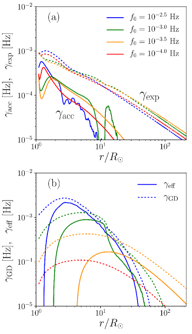
Figure 3: a: Decay rates of density fluctuation due to wind acceleration $\gamma_{\rm acc}$ (solid line) and due to wind expansion $\gamma_{\rm exp}$ (dashed line). b: Growth rate of PDI given by the Goldstein–Derby dispersion relation $\gamma_{\rm GD}$ (dashed line) and the effective growth rate $\gamma_{\rm eff}$ (solid line). Blue, green, orange, and red lines indicate $f_{0}=10^{-2.5}{\rm\ Hz}$, $10^{-3.0}{\rm\ Hz}$, $10^{-3.5}{\rm\ Hz}$, and $10^{-4.0}{\rm\ Hz}$, respectively. We note that $\gamma_{\rm eff}$ of $f_{0}=10^{-4.0}{\rm\ Hz}$ (red solid) is negative in the entire region.

3.3 Doppler effect and effective growth rate

To discuss the possibility of the onset of PDI for each $f_{0}$, we calculated $\gamma_{\rm eff}$ using Eq. (39). The normalized growth rate $\gamma_{\rm GD}/\omega$ was calculated from Eq. (3). We should note that $\omega\neq 2\pi f_{0}$ because of the Doppler effect by the acceleration of the solar wind. $\omega$ should be the intrinsic frequency, that is, the wave frequency observed in a co-moving frame of the solar wind. Because the wave frequency observed from a fixed coordinate is constant in a quasi-steady state, the wave number $k(r)$ satisfies

$$k(r)=\frac{2\pi f_{0}}{v_{A}(r)+v_{r}(r)}.$$ (40)

When we observed this wave in a co-moving frame, the wave number was invariant and the phase speed decreased to $v_{A}(r)$, and therefore,

$$\omega=v_{A}(r)k(r)=2\pi f_{0}\frac{v_{A}(r)}{v_{A}(r)+v_{r}(r)}.$$ (41)

This means that the intrinsic frequency decreases in an accelerating flow. In the accelerating expanding box model, this effect is mentioned as the box-stretching effect (Tenerani & Velli, 2017). A similar argument appears in deriving the wave-action conservation (Dewar, 1970; Heinemann & Olbert, 1980).

We should note that, the wind-acceleration effect appears in different ways. As discussed in Section 3.2, the wind acceleration works to reduce the density fluctuation. In addition, as discussed here, wind acceleration also causes the Doppler effect.

In Figure 3, we show $\gamma_{\rm eff}$, $\gamma_{\rm GD}$, $\gamma_{\rm acc}$, and $\gamma_{\rm exp}$ as functions of height to see the effects of wind acceleration and expansion on the growth rate of PDI. $\gamma_{\rm acc}$ (solid lines) and $\gamma_{\rm exp}$ (dashed lines) are shown in Figure 3a, while $\gamma_{\rm eff}$ and $\gamma_{\rm GD}$ are shown in Figure 3b. The colors represent the injection frequency as follows: $f_{0}=10^{-2.5}{\rm\ Hz}$ (blue), $f_{0}=10^{-3.0}{\rm\ Hz}$ (green), $f_{0}=10^{-3.5}{\rm\ Hz}$ (orange), and $f_{0}=10^{-4.0}{\rm\ Hz}$ (red). Figure 3a shows that the expansion ($\gamma_{\rm exp}$) dominates the acceleration ($\gamma_{\rm acc}$) in the damping of the PDI. As a result, $\gamma_{\rm GD}$ is reduced to $\gamma_{\rm eff}$. The reduction factors, $\gamma_{\rm acc}/\gamma_{\rm GD}$ and $\gamma_{\rm exp}/\gamma_{\rm GD}$, are larger for smaller injection frequencies, $f_{0}$, because $\gamma_{\rm GD}$ is proportional to $f_{0}$. Specifically when $f_{0}=10^{-4.0}{\rm\ Hz}$, $\gamma_{\rm GD}$ is smaller than the reduction factor, $\gamma_{\rm acc}+\gamma_{\rm exp}$, and the effective growth rate is negative. The local maxima of $\gamma_{\rm GD}$ is determined by the balance between plasma beta and wave amplitude (see Eq. (1)); the plasma beta is low and the wave amplitude is small in the lower corona and vice versa in the distant solar wind.

3.4 Onset and suppression of PDI

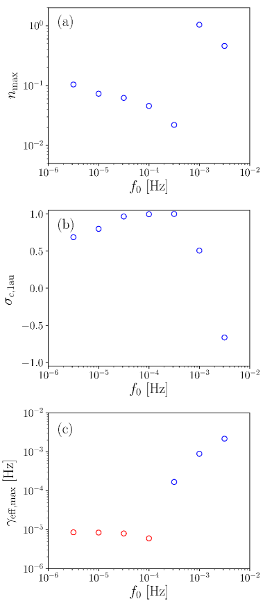
Figure 4: Solar wind parameters versus wave-injection frequency $f_{0}$. Each panel indicates a: maximum fractional density fluctuation $n$, b: normalized cross-helicity $\sigma_{c}$ at $1{\rm\ au}$, c: maximum effective growth rate $\gamma_{\rm eff}$ (blue: positive, red: negative).

To discuss the threshold of the onset of PDI, we calculated the maximum fractional density fluctuation $n_{\rm max}$ and the normalized cross-helicity (Alfvénicity) $\sigma_{c}$ at $1{\rm\ au}$. Here we defined $n_{\rm max}$ and $\sigma_{c}$ as

$$n_{\rm max} =\max\left(\frac{1}{\rho_{\rm ave}}\sqrt{\langle\left(\rho-\rho_{\rm ave}\right)^{2}\rangle}\right),\ \ \ \ \rho_{\rm ave}=\langle\rho\rangle,$$ (42)

$$\sigma_{c} =\frac{\langle z^{+}\rangle^{2}-\langle z^{-}\rangle^{2}}{\langle z^{+}\rangle^{2}+\langle z^{-}\rangle^{2}},$$ (43)

where $\langle X\rangle$ denotes the time-averaged value of $X$ and $\max\left(X\right)$ denotes the maximum value of $X$ in space. We note that the sign of ${\sigma_{c}}$ is opposite to the sign of $H_{c}=\mbox{\boldmath$v$}\cdot\mbox{\boldmath$B$}$. These values can be useful indicators of PDI because PDI generates large-amplitude density fluctuation, which increases $n$, and back-scattered Alfvén waves, which reduce $\sigma_{c}$. The latter effect works to reduce $\sigma_{c}$. According to Cranmer & van Ballegooijen (2012), without PDI, $\delta\rho_{\rm rms}/\rho_{0}\lesssim 0.1$, and thus $\delta\rho_{\rm rms}/\rho_{0}>0.1$ indicates the PDI.

In Figure 4, we show a: $n_{\rm max}$, b: $\sigma_{c}$ at $1{\rm\ au}$, and c: the maximum effective growth rate $\gamma_{\rm eff,max}$ (blue: positive, red: negative) as functions of $f_{0}$. When $f_{0}\lesssim 10^{-3.5}{\rm\ Hz}$, both $n_{\rm max}$ and $\sigma_{c}$ show monotonic trends with $f_{0}$: $n_{\rm max}$ decreases and $\sigma_{c}$ increases as $f_{0}$ increases. This is explained as follows. As $f_{0}$ becomes smaller, Alfvén waves are reflected more efficiently (Ferraro & Plumpton, 1958; An et al., 1990; Velli, 1993; Cranmer & van Ballegooijen, 2005; Hollweg & Isenberg, 2007). If Alfvén waves are reflected in the solar wind beyond the Alfvén point, reflected Alfvén waves are advected towards $1{\rm\ au}$ and contribute to reducing $\sigma_{c}$. Note that the inward waves vanish near the Alfvén point (Verdini et al., 2009; Tenerani & Velli, 2017). When the amount of reflected Alfvén waves increases, the interaction between outward and inward waves is activated. This wave-wave collision excites not only turbulence (Iroshnikov, 1964; Kraichnan, 1965; Dobrowolny et al., 1980; Goldreich & Sridhar, 1995), but also the slow-mode generation (Wentzel, 1974; Uchida & Kaburaki, 1974) by the modulation of magnetic field pressure (Hollweg, 1971; Kudoh & Shibata, 1999; Cranmer & Woolsey, 2015). Magnetic field modulation also leads to direct steepening to fast shock (Cohen & Kulsrud, 1974; Kennel et al., 1990; Suzuki, 2004). Owing to these processes, larger-density fluctuation is likely to be generated in the presence of larger-amplitude reflected Alfvén waves.

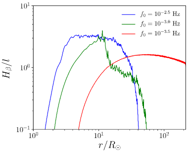
Figure 5: Scale ratio $H_{\beta}/l$ where $l$ and $H_{\beta}$ denote the typical propagation length scale during the PDI growth and the scale length of plasma beta, respectively. Blue, green, and red lines indicate $f_{0}=10^{-2.5}{\rm\ Hz}$, $10^{-3.0}{\rm\ Hz}$, and $10^{-3.5}{\rm\ Hz}$, respectively.

The monotonic trend in $10^{-5.5}{\rm\ Hz}\lesssim f_{0}\lesssim 10^{-3.5}{\rm\ Hz}$ breaks down near $f_{0}\approx 10^{-3}{\rm\ Hz}$. When $f_{0}$ gets larger than $10^{-3}{\rm\ Hz}$, $n_{\rm max}$ becomes larger than $0.1$ and $\sigma_{c}$ becomes smaller than $0.5$. Considering the fact that PDI generates large amounts of density fluctuation and reflected Alfvén waves, Figure 4 indicates that the frequency threshold of the onset of PDI is $10^{-3.5}{\rm\ Hz}<f_{0}<10^{-3}{\rm\ Hz}$. This means that, even though $\gamma_{\rm eff,max}$ is positive when $f_{0}=10^{-3.5}{\rm\ Hz}$, PDI cannot develop with this injection frequency. Tenerani & Velli (2013) argued that PDI is suppressed not only by the acceleration and expansion of the solar wind but also by the inhomogeneity of the solar wind, because the resonance condition changes as the plasma parameters such as the plasma beta, Alfvén speed and wave amplitude, vary. In Figure 5, we show the ratio between the propagation length during growth time $l$ and the scale length of the plasma beta ($H_{\beta}$):

$$l=\frac{v_{A}+v_{r}}{\gamma_{\rm eff}},\ \ \ \ H_{\beta}=\left|\frac{\beta}{\partial\beta/\partial r}\right|.$$ (44)

The ratio, $H_{\beta}/l$, can be used as a measure of how the inhomogeneity of the background field affects the onset of PDI; if $H_{\beta}/l$ is small $\lesssim 1$, the background inhomogeneity could suppress the PDI. Figure 5 shows $H_{\beta}/l$ versus height. This indicates that, when $f_{0}=10^{-3.5}{\rm\ Hz}$, PDI cannot evolve because the scale ratio $H_{\beta}/l$ is at most around unity and the inhomogeneity affects the growth of PDI.

Another possible reason that PDI is not observed when $f_{0}=10^{-3.5}{\rm\ Hz}$ is that the typical growth time is too small to develop before $1{\rm\ au}$. $\gamma_{\rm eff}$ averaged over the entire simulation box is approximately $\overline{\gamma}_{\rm eff}=5\times 10^{-5}{\rm\ Hz}$, corresponding to the timescale of $\overline{\tau}=2\times 10^{4}{\rm\ s}$. Therefore, because it takes a few $\overline{\tau}$ to reach the saturation phase of PDI, the evolution timescale ($\sim 10^{5}{\rm\ s}$) is comparable to the propagation timescale up to $1{\rm\ au}$ ($\sim 2\times 10^{5}{\rm\ s}$). This indicates that $1{\rm\ au}$ might be too short for the PDI of $f_{0}=10^{-3.5}{\rm\ Hz}$ to develop.

4 Broadband-wave injection

Next, we applied the broadband-wave injection to discuss the consistency with observation. The boundary condition is given as

$$z^{+}_{x,y}=\int^{f_{\rm max}}_{f_{\rm min}}P(f)\sin\left(2\pi ft+\phi_{x,y}(f)\right)df,$$ (45)

where $P(f)$ is determined so that the root-mean-square value is $2v_{\rm rms,0}$ and the power show $1/f$ spectrum in $f_{\rm min}\leq f\leq f_{\rm max}$ (Bruno & Carbone, 2013). $\phi_{x,y}(f)$ are random functions of $f$. We fixed $f_{\rm max}=10^{-2}{\rm\ Hz}$, corresponding to $100{\rm\ s}$ in terms of period. Note that some observations show an even higher frequency component (He et al., 2009; Okamoto & De Pontieu, 2011; Shoda & Yokoyama, 2018). $f_{\rm min}$ is the free parameter. In this study, we calculated three cases: $f_{\rm min}=10^{-3}{\rm\ Hz}$, $10^{-4}{\rm\ Hz}$, $10^{-5}{\rm\ Hz}$, each of which corresponded to the largest timescale of the photospheric transverse motion (Matsumoto & Kitai, 2010), the coronal transverse motion (Morton et al., 2015), and the solar-wind fluctuations (Tu & Marsch, 1995), respectively.

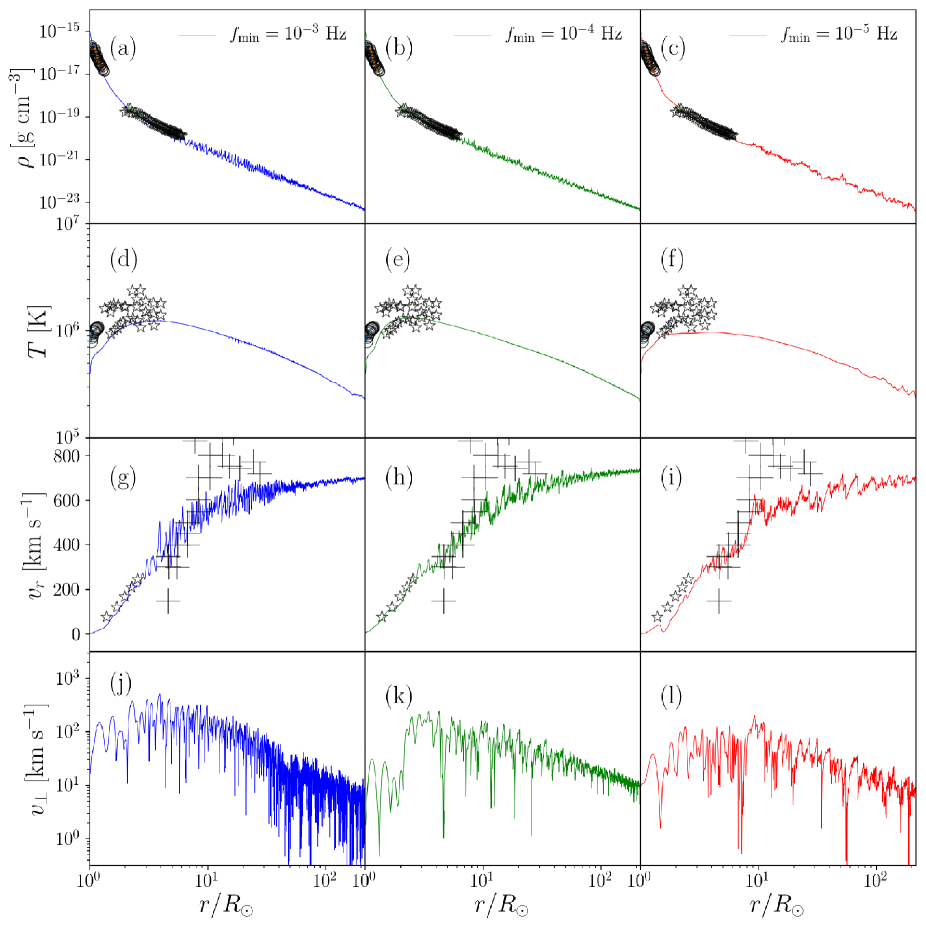
Figure 6: Quasi-steady states with different $f_{\rm min}$ values. Blue, green and red lines indicate $f_{\rm min}=10^{-3}{\rm\ Hz}$, $10^{-4}{\rm\ Hz}$, $10^{-5}{\rm\ Hz}$, respectively. a-c: mass density. Shown by circles and stars are observations by Wilhelm et al. (1998) and by Lamy et al. (1997), respectively. d-f: temperature. Shown by circles and stars are observations by Landi (2008) and compilation of observed data by Cranmer (2004, 2009), respectively. g-i: radial velocity. Shown by stars are ion outflow speed by Zangrilli et al. (2002), while the crosses represent the IPS observations (Kojima et al., 2004). j-l: transverse velocity (Alfvén-wave amplitude).

4.1 Quasi-steady state

As in Section 3, we begin by discussing the quasi-steady states. Figure 6 shows the same variables as those shown in Figure 1 except for Panel d, where the transverse velocity $v_{\perp}$ is shown instead of the Elsässer variables. Color represents $f_{\rm min}=10^{-3}{\rm\ Hz}$ (blue), $10^{-4}{\rm\ Hz}$ (green), $10^{-5}{\rm\ Hz}$ (red), respectively. Because the main motivation of broadband-wave injection is to compare to observations, we also show several observational values. In Panel a, we show the density observation by Wilhelm et al. (1998) (circles) and Lamy et al. (1997) (stars). In converting the observed electron density $n_{e}$ to mass density $\rho$, we simply assumed $\rho=m_{p}n_{e}$. In Panel b, circles and stars correspond to the results from Landi (2008) and Cranmer (2004, 2009), respectively. In Panel c, observed ion-outflow velocity is plotted by stars (Zangrilli et al., 2002), while the results of IPS observation are indicated by crosses (Kojima et al., 2004).

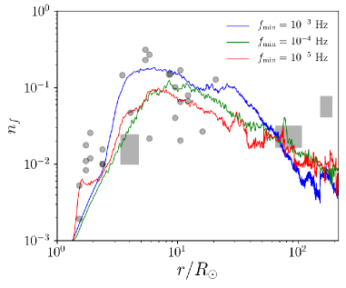
Figure 7: Fractional density fluctuation $n_{f}$ versus heliocentric distance. Blue, green and red lines indicate $f_{\rm min}=10^{-3}{\rm\ Hz}$, $10^{-4}{\rm\ Hz}$, $10^{-5}{\rm\ Hz}$, respectively. Shown by gray rectangles and circles are the observational values (see text).

4.2 Density fluctuation

The density fluctuation in the solar wind is observed by radio-wave observation. As explained in the Introduction, density fluctuation possibly plays a role in reflecting Alfvén waves in the corona and solar wind (van Ballegooijen & Asgari-Targhi, 2016).

When we applied the broadband-wave injection, it was difficult to obtain the amplitude of the density fluctuation that was solely attributed to PDI, because the density fluctuates not only by PDI but also by the time variation of the injected energy flux. Since the density fluctuation that comes from the injection has a timescale of typically $f_{\rm min}$, in this study, we defined the density fluctuation as high-frequency ($>f_{\rm min}$) components. Given that we have density $\rho(r,t)$, the fractional fluctuation $n_{f}(r)$ is given as

$$n_{f}(r)=\frac{1}{\rho_{\rm ave}}\sqrt{\frac{1}{2\pi\tau_{0}}\int_{\left|\omega\right|>2\pi f_{\rm th}}\left|\tilde{\rho}(r,\omega)\right|^{2}d\omega},$$ (46)

where

$$\tilde{\rho}(r,\omega)=\int^{\tau_{0}}_{0}dt\rho(r,t)e^{i\omega t}.$$ (47)

Note that Parseval’s identity holds as follows:

$$\int dt\left|\rho(r,t)\right|^{2}=\frac{1}{2\pi}\int d\omega\left|\tilde{\rho}\left(r,\omega\right)\right|^{2}.$$ (48)

$f_{\rm th}$ is the frequency threshold. Here, we set $f_{\rm th}=10^{-3}{\rm\ Hz}$. Although this value was a rather arbitrary choice, we confirmed that the radial trend of $n_{f}$ does not depend on $f_{\rm th}$.

Figure 7 shows the radial profiles of $n_{f}(r)$. Rectangles are observational values taken from Cranmer & van Ballegooijen (2012). The rectangle near $r=5R_{\odot}$ indicates the radio sounding data (Coles & Harmon, 1989; Spangler, 2002; Harmon & Coles, 2005) while the rectangles in $r\gtrsim 100R_{\odot}$ indicate the in-situ data by Marsch & Tu (1990). The circles indicate the observation by Miyamoto et al. (2014).

Our three cases nicely explain the overall radial profile of the observed density fluctuation peaked at $r\sim 5-10R_{\odot}$ (Miyamoto et al., 2014). The peak of $n_{f}$ in our calculation is created by the high-frequency ($f>10^{-3.5}$Hz) Alfvén waves that are subject to PDI (Fig.3b). The largest effective growth rate $\gamma_{\rm eff}$ is peaked in $r\sim 2-10R_{\odot}$ when the parent-wave frequency is $10^{-3}-10^{-2}{\rm\ Hz}$. Therefore, the large density fluctuations are excited as an outcome of the PDI in these locations. To summarize, the observed density fluctuation is explained by the evolution of the PDI of high-frequency ($10^{-2}-10^{-3}{\rm\ Hz}$) Alfvén waves.

4.3 Cross-helicity in the solar wind

Because the radial evolution of Elsässer variables $z^{\pm}$ in the heliosphere has been observed (Bavassano et al., 1982, 2000), we can test our theoretical model by comparison with these observations. In Figure 8, we show the radial profile of time-averaged Elsässer variables ($z^{+}$: solid line, $z^{-}$: dashed line) with different $f_{\rm min}$ values ($f_{\rm min}=10^{-3}{\rm\ Hz}$: blue, $10^{-4}{\rm\ Hz}$: green, $10^{-5}{\rm\ Hz}$: red). Also shown by gray transparent lines are the observational trends by Bavassano et al. (2000).

While $z^{+}$ is consistent with observation when $f_{\rm min}=10^{-4},\ 10^{-5}{\rm\ Hz}$, we have a much smaller $z^{+}$ compared with observation when $f_{\rm min}=10^{-3}{\rm\ Hz}$. Because PDI evolves when $f_{0}\gtrsim 10^{-3}{\rm Hz}$, this discrepancy indicates that, via PDI, excessive energy transfer from $z^{+}$ to $z^{-}$ occurs. When $f_{\rm min}$ becomes smaller, the intensity of high-frequency waves that are subject to PDI is reduced because the total wave power is fixed. This is why the signature of PDI is weak for smaller $f_{0}$. Our result indicates that the cross-helicity evolution in the solar wind is dominated by the linear reflection (Zhou & Matthaeus, 1990; Velli et al., 1991; Verdini & Velli, 2007). Because the simulated $z^{-}$ approaches the observational value as $f_{\rm min}$ decreases, as a result of PDI suppression, the cross-helicity evolution in the solar wind is governed by linear reflection of low-frequency ($f_{0}\sim 10^{-5}{\rm\ Hz}$) components.

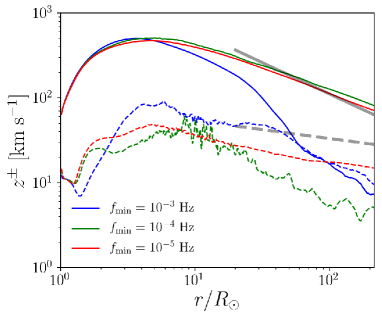
Figure 8: Radial profiles of time-averaged Elsässer variables. Solid and dashed lines indicate $z^{+}$ (anti-sunward) and $z^{-}$ (sunward) components. Blue, green and red lines indicate $f_{\rm min}=10^{-3}{\rm\ Hz}$, $10^{-4}{\rm\ Hz}$, $10^{-5}{\rm\ Hz}$, respectively. Also shown by gray lines are observational trends by Bavassano et al. (2000).

5 Summary & Discussion

In this study, using numerical simulations, we investigated the threshold of the onset of PDI by changing the Alfvén-wave injection. As discovered by Tenerani & Velli (2013) and Del Zanna et al. (2015), wind acceleration and expansion work to reduce the growth rate of PDI. We have solved the wave propagation self-consistently from the coronal base to $1{\rm\ au}$, and this was then compared with the accelerating expanding box simulation.

Firstly, we investigated the fundamental processes of PDI by applying monotonic-wave injection with frequency $f_{0}$. Our results show that PDI can develop when $f_{0}\gtrsim 10^{-3}{\rm\ Hz}$, while we observe no signature of PDI when $f_{0}\lesssim 10^{-3.5}{\rm\ Hz}$. Owing to the wind acceleration and expansion, the growth rate of PDI becomes negative when $f_{0}\lesssim 10^{-4.0}{\rm\ Hz}$. When $f_{0}\lesssim 10^{-3.5}{\rm\ Hz}$, even though the growth rate of PDI is positive, PDI cannot develop. The suppression by solar wind inhomogeneity or the long timescale of growth might be the reason for this.

The frequency-filtering mechanism can operate in the corona and solar wind due to the bimodal behavior of wave dissipation with respect to frequency. The low-frequency ($f_{0}\lesssim 10^{-4}{\rm\ Hz}$) waves undergo linear reflection and generate Alfvénic turbulence from the interaction with counter-propagating waves. The high-frequency ($f_{0}\gtrsim 10^{-3}{\rm\ Hz}$) waves dissipate through the PDI. As a result of the efficient heating, dense, hot and relatively slow winds are driven in the cases with $f_{0}\lesssim 10^{-4}{\rm\ Hz}$ or $f_{0}\gtrsim 10^{-3}{\rm\ Hz}$. In contrast, the intermediate-frequency ($f_{0}\approx 10^{-3.5}{\rm\ Hz}$) waves are not severely subjected to these damping mechanisms. As a result, fast and less dense wind emanates from the relatively cool corona in this case. This indicates that the corona and solar wind have a frequency-filtering effect of the Alfvén wave, and as a result, the medium-frequency wave is likely to permeate. This is a possible reason for the hour-scale waves observed in the solar wind (Belcher & Davis, 1971).

Secondly, we applied broadband-wave injection to compare the numerical results with observation. The observed radial trend of the density fluctuation can be well explained by the evolution of the high-frequency ($f_{0}\gtrsim 10^{-3}{\rm\ Hz}$) Alfvén waves. However, the observed trend of the cross-helicity can be explained by the linear reflection of the low-frequency ($f_{0}<10^{-4}{\rm\ Hz}$) Alfvén waves. These results show that the Alfvén waves in a wide range of frequency play an essential role in the global solar wind.

There are several limitations in our model. The most severe limitation is the treatment of turbulence. We have applied a simple one-point-closure model of Alfvén wave turbulence (Eq. (14) and (17)) with the correlation length that increases with an expanding flux tube (Eq. (19)). However, Cranmer & van Ballegooijen (2012) showed that Eq. (19) possibly underestimates the correlation length. To overcome this, we needed to solve the transport equation of $\lambda$ (Breech et al., 2008; Usmanov et al., 2011). In addition, the correlation length should be different between $z^{+}$ and $z^{-}$ (Zank et al., 2017; Shiota et al., 2017). More sophisticated treatment of the turbulence, including the shell model (Buchlin & Velli, 2007; Verdini et al., 2012), remains as a future work.

Another limitation is one-dimensional modeling. While the Alfvén wave turbulence is taken into account phenomenologically, we completely ignore the effect of phase mixing (Heyvaerts & Priest, 1983; Kaneko et al., 2015; Antolin et al., 2015; Okamoto et al., 2015) by 1D modeling. Besides, it has been shown by Del Zanna et al. (2001) that the onset (and possibly growth) of parametric decay instability is slower in 3D than in 1D. Our quantitative discussion might be slightly modified by the 1D assumption. Also, we cannot take into account the wave refraction in the lower region (Rosenthal et al., 2002; Bogdan et al., 2003). In future, we need to conduct a 3D MHD simulation for the reasons above.

In this study, we have focused on the frequency dependence. Since the growth rate of parametric decay instability depends also on plasma beta and wave amplitude (Goldstein, 1978; Derby, 1978). Suzuki & Inutsuka (2006) investigated the dependence on the injected wave amplitude. Readers probably expect that the PDI is suppressed for smaller wave injection according to Eq. (1). However, the response of the solar wind totally changes the situation. A case with smaller injection gives lower coronal temperature because of the suppressed heating. As a result, the plasma beta in the corona is lower, and larger density fluctuations are excited by more activated PDI as shown in Figure 9 of Suzuki & Inutsuka (2006). Similarly, it is expected that the density variation is large when the magnetic field is stronger and the plasma beta is lower.

There are also ambiguities in the thermal flux in the free-streaming regime. We chose $\alpha=2$ in evaluating the magnitude of free-streaming thermal flux. Although $\alpha=4$ has been sometimes used (Leer et al., 1982; Withbroe, 1988; Landi & Pantellini, 2003; Cranmer et al., 2007; van Ballegooijen & Asgari-Targhi, 2016), $\alpha=4$ might overestimate the actual flux because thermal conduction can be suppressed by the local instability and turbulence (Gary et al., 1999; Roberg-Clark et al., 2017; Komarov et al., 2017; Tong et al., 2018). Indeed Cranmer et al. (2009) showed that $\alpha=1.05$ yields good agreement with observation, and several recent studies used $\alpha=1.05$ (Usmanov et al., 2011; van der Holst et al., 2014). The precise value of $\alpha$ should depend on the solar wind condition. Since the change in $\alpha$ does not strongly affect the physical quantities of the solar wind (Cranmer et al., 2007), we expect that our findings are independent on $\alpha$.

M.S. is supported by the Leading Graduate Course for Frontiers of Mathematical Sciences and Physics (FMSP) and Grant-in-Aid for Japan Society for the Promotion of Science (JSPS) Fellows. T.Y. is supported by JSPS KAKENHI Grant Number 15H03640. T.K.S. is supported in part by Grants-in-Aid for Scientific Research from the MEXT of Japan, 17H01105. Numerical calculations were in part carried out on the PC cluster at the Center for Computational Astrophysics, National Astronomical Observatory of Japan.

References

- Alfvén (1942) Alfvén, H. 1942, Nature, 150, 405
- Alfvén (1947) —. 1947, MNRAS, 107, 211
- An et al. (1990) An, C.-H., Suess, S. T., Moore, R. L., & Musielak, Z. E. 1990, ApJ, 350, 309
- Antolin et al. (2015) Antolin, P., Okamoto, T. J., De Pontieu, B., Uitenbroek, H., Van Doorsselaere, T., & Yokoyama, T. 2015, ApJ, 809, 72
- Arge & Pizzo (2000) Arge, C. N., & Pizzo, V. J. 2000, J. Geophys. Res., 105, 10465
- Banerjee et al. (2009) Banerjee, D., Pérez-Suárez, D., & Doyle, J. G. 2009, A&A, 501, L15
- Bavassano et al. (1982) Bavassano, B., Dobrowolny, M., Mariani, F., & Ness, N. F. 1982, J. Geophys. Res., 87, 3617
- Bavassano et al. (2000) Bavassano, B., Pietropaolo, E., & Bruno, R. 2000, J. Geophys. Res., 105, 15959
- Belcher (1971) Belcher, J. W. 1971, ApJ, 168, 509
- Belcher & Davis (1971) Belcher, J. W., & Davis, Jr., L. 1971, J. Geophys. Res., 76, 3534
- Bogdan et al. (2003) Bogdan, T. J., et al. 2003, ApJ, 599, 626
- Bourdin (2017) Bourdin, P.-A. 2017, ApJ, 850, L29
- Bowen et al. (2018) Bowen, T. A., Badman, S., Hellinger, P., & Bale, S. D. 2018, ApJ, 854, L33
- Breech et al. (2008) Breech, B., Matthaeus, W. H., Minnie, J., Bieber, J. W., Oughton, S., Smith, C. W., & Isenberg, P. A. 2008, Journal of Geophysical Research (Space Physics), 113, A08105
- Bruno & Carbone (2013) Bruno, R., & Carbone, V. 2013, Living Reviews in Solar Physics, 10, 2
- Buchlin & Velli (2007) Buchlin, E., & Velli, M. 2007, ApJ, 662, 701
- Chandran (2018) Chandran, B. D. G. 2018, Journal of Plasma Physics, 84, 905840106
- Chandran & Hollweg (2009) Chandran, B. D. G., & Hollweg, J. V. 2009, ApJ, 707, 1659
- Cohen & Dewar (1974) Cohen, R. H., & Dewar, R. L. 1974, J. Geophys. Res., 79, 4174
- Cohen & Kulsrud (1974) Cohen, R. H., & Kulsrud, R. M. 1974, Physics of Fluids, 17, 2215
- Coleman (1968) Coleman, Jr., P. J. 1968, ApJ, 153, 371
- Coles & Harmon (1989) Coles, W. A., & Harmon, J. K. 1989, ApJ, 337, 1023
- Cranmer (2004) Cranmer, S. R. 2004, in ESA Special Publication, Vol. 575, SOHO 15 Coronal Heating, ed. R. W. Walsh, J. Ireland, D. Danesy, & B. Fleck, 154
- Cranmer (2009) Cranmer, S. R. 2009, Living Reviews in Solar Physics, 6, 3
- Cranmer et al. (2009) Cranmer, S. R., Matthaeus, W. H., Breech, B. A., & Kasper, J. C. 2009, ApJ, 702, 1604
- Cranmer & van Ballegooijen (2005) Cranmer, S. R., & van Ballegooijen, A. A. 2005, ApJS, 156, 265
- Cranmer & van Ballegooijen (2012) —. 2012, ApJ, 754, 92
- Cranmer et al. (2007) Cranmer, S. R., van Ballegooijen, A. A., & Edgar, R. J. 2007, ApJS, 171, 520
- Cranmer & Woolsey (2015) Cranmer, S. R., & Woolsey, L. N. 2015, ApJ, 812, 71
- De Groof & Goossens (2002) De Groof, A., & Goossens, M. 2002, A&A, 386, 691
- De Pontieu et al. (2007) De Pontieu, B., et al. 2007, Science, 318, 1574
- Del Zanna et al. (2015) Del Zanna, L., Matteini, L., Landi, S., Verdini, A., & Velli, M. 2015, Journal of Plasma Physics, 81, 325810102
- Del Zanna et al. (2001) Del Zanna, L., Velli, M., & Londrillo, P. 2001, A&A, 367, 705
- Derby (1978) Derby, Jr., N. F. 1978, ApJ, 224, 1013
- Dewar (1970) Dewar, R. L. 1970, Physics of Fluids, 13, 2710
- Dmitruk & Matthaeus (2003) Dmitruk, P., & Matthaeus, W. H. 2003, ApJ, 597, 1097
- Dmitruk et al. (2002) Dmitruk, P., Matthaeus, W. H., Milano, L. J., Oughton, S., Zank, G. P., & Mullan, D. J. 2002, ApJ, 575, 571
- Dobrowolny et al. (1980) Dobrowolny, M., Mangeney, A., & Veltri, P. 1980, Physical Review Letters, 45, 144
- Dorfman & Carter (2016) Dorfman, S., & Carter, T. A. 2016, Physical Review Letters, 116, 195002
- Elsässer (1950) Elsässer, W. M. 1950, Physical Review, 79, 183
- Ferraro & Plumpton (1958) Ferraro, C. A., & Plumpton, C. 1958, ApJ, 127, 459
- Fu et al. (2017) Fu, X., Li, H., Guo, F., Li, X., & Roytershteyn, V. 2017, ArXiv e-prints
- Fujiki et al. (2015) Fujiki, K., Tokumaru, M., Iju, T., Hakamada, K., & Kojima, M. 2015, Sol. Phys., 290, 2491
- Galeev & Oraevskii (1963) Galeev, A. A., & Oraevskii, V. N. 1963, Soviet Physics Doklady, 7, 988
- Gary (2001) Gary, G. A. 2001, Sol. Phys., 203, 71
- Gary et al. (1999) Gary, S. P., Neagu, E., Skoug, R. M., & Goldstein, B. E. 1999, J. Geophys. Res., 104, 19843
- Ghosh & Goldstein (1994) Ghosh, S., & Goldstein, M. L. 1994, J. Geophys. Res., 99, 13
- Ghosh et al. (1994) Ghosh, S., Vinas, A. F., & Goldstein, M. L. 1994, J. Geophys. Res., 99, 19
- Goldreich & Sridhar (1995) Goldreich, P., & Sridhar, S. 1995, ApJ, 438, 763
- Goldstein (1978) Goldstein, M. L. 1978, ApJ, 219, 700
- Goossens et al. (2012) Goossens, M., Andries, J., Soler, R., Van Doorsselaere, T., Arregui, I., & Terradas, J. 2012, ApJ, 753, 111
- Grappin & Velli (1996) Grappin, R., & Velli, M. 1996, J. Geophys. Res., 101, 425
- Grappin et al. (1993) Grappin, R., Velli, M., & Mangeney, A. 1993, Physical Review Letters, 70, 2190
- Hahn & Savin (2013) Hahn, M., & Savin, D. W. 2013, ApJ, 776, 78
- Hansteen & Velli (2012) Hansteen, V. H., & Velli, M. 2012, Space Sci. Rev., 172, 89
- Harmon & Coles (2005) Harmon, J. K., & Coles, W. A. 2005, Journal of Geophysical Research (Space Physics), 110, A03101
- He et al. (2009) He, J.-S., Tu, C.-Y., Marsch, E., Guo, L.-J., Yao, S., & Tian, H. 2009, A&A, 497, 525
- Heinemann & Olbert (1980) Heinemann, M., & Olbert, S. 1980, J. Geophys. Res., 85, 1311
- Heyvaerts & Priest (1983) Heyvaerts, J., & Priest, E. R. 1983, A&A, 117, 220
- Hollweg (1971) Hollweg, J. V. 1971, J. Geophys. Res., 76, 5155
- Hollweg (1974) —. 1974, J. Geophys. Res., 79, 3845
- Hollweg (1976) —. 1976, J. Geophys. Res., 81, 1649
- Hollweg et al. (1982) Hollweg, J. V., Bird, M. K., Volland, H., Edenhofer, P., Stelzried, C. T., & Seidel, B. L. 1982, J. Geophys. Res., 87, 1
- Hollweg et al. (2010) Hollweg, J. V., Cranmer, S. R., & Chandran, B. D. G. 2010, ApJ, 722, 1495
- Hollweg & Isenberg (2007) Hollweg, J. V., & Isenberg, P. A. 2007, Journal of Geophysical Research (Space Physics), 112, 8102
- Hoshino & Goldstein (1989) Hoshino, M., & Goldstein, M. L. 1989, Physics of Fluids B, 1, 1405
- Hossain et al. (1995) Hossain, M., Gray, P. C., Pontius, Jr., D. H., Matthaeus, W. H., & Oughton, S. 1995, Physics of Fluids, 7, 2886
- Iroshnikov (1964) Iroshnikov, P. S. 1964, Soviet Ast., 7, 566
- Iwai et al. (2014) Iwai, K., Shibasaki, K., Nozawa, S., Takahashi, T., Sawada, S., Kitagawa, J., Miyawaki, S., & Kashiwagi, H. 2014, Earth, Planets, and Space, 66, 149
- Jacques (1977) Jacques, S. A. 1977, ApJ, 215, 942
- Jayanti & Hollweg (1993) Jayanti, V., & Hollweg, J. V. 1993, J. Geophys. Res., 98, 19
- Kaneko et al. (2015) Kaneko, T., Goossens, M., Soler, R., Terradas, J., Van Doorsselaere, T., Yokoyama, T., & Wright, A. N. 2015, ApJ, 812, 121
- Kennel et al. (1990) Kennel, C. F., Blandford, R. D., & Wu, C. C. 1990, Physics of Fluids B, 2, 253
- Kojima et al. (2004) Kojima, M., Breen, A. R., Fujiki, K., Hayashi, K., Ohmi, T., & Tokumaru, M. 2004, Journal of Geophysical Research (Space Physics), 109, A04103
- Komarov et al. (2017) Komarov, S., Schekochihin, A., Churazov, E., & Spitkovsky, A. 2017, ArXiv e-prints
- Kopp & Holzer (1976) Kopp, R. A., & Holzer, T. E. 1976, Sol. Phys., 49, 43
- Kraichnan (1965) Kraichnan, R. H. 1965, Physics of Fluids, 8, 1385
- Kudoh & Shibata (1999) Kudoh, T., & Shibata, K. 1999, ApJ, 514, 493
- Lamy et al. (1997) Lamy, P., Quemerais, E., Llebaria, A., Bout, M., Howard, R., Schwenn, R., & Simnett, G. 1997, in ESA Special Publication, Vol. 404, Fifth SOHO Workshop: The Corona and Solar Wind Near Minimum Activity, ed. A. Wilson, 491
- Landi (2008) Landi, E. 2008, ApJ, 685, 1270
- Landi & Pantellini (2003) Landi, S., & Pantellini, F. 2003, A&A, 400, 769
- Lashmore-Davies (1976) Lashmore-Davies, C. N. 1976, Physics of Fluids, 19, 587
- Leer et al. (1982) Leer, E., Holzer, T. E., & Fla, T. 1982, Space Sci. Rev., 33, 161
- Levine et al. (1977) Levine, R. H., Altschuler, M. D., Harvey, J. W., & Jackson, B. V. 1977, ApJ, 215, 636
- Lionello et al. (2014) Lionello, R., Velli, M., Downs, C., Linker, J. A., Mikić, Z., & Verdini, A. 2014, ApJ, 784, 120
- Magyar et al. (2017) Magyar, N., Van Doorsselaere, T., & Goossens, M. 2017, Scientific Reports, 7, 14820
- Malara et al. (2000) Malara, F., Primavera, L., & Veltri, P. 2000, Physics of Plasmas, 7, 2866
- Malara & Velli (1996) Malara, F., & Velli, M. 1996, Physics of Plasmas, 3, 4427
- Marsch & Tu (1990) Marsch, E., & Tu, C.-Y. 1990, J. Geophys. Res., 95, 11945
- Matsumoto & Kitai (2010) Matsumoto, T., & Kitai, R. 2010, ApJ, 716, L19
- Matsumoto & Suzuki (2012) Matsumoto, T., & Suzuki, T. K. 2012, ApJ, 749, 8
- Matsumoto & Suzuki (2014) —. 2014, MNRAS, 440, 971
- Matthaeus et al. (1999) Matthaeus, W. H., Zank, G. P., Oughton, S., Mullan, D. J., & Dmitruk, P. 1999, ApJ, 523, L93
- McIntosh et al. (2011) McIntosh, S. W., de Pontieu, B., Carlsson, M., Hansteen, V., Boerner, P., & Goossens, M. 2011, Nature, 475, 477
- Miyamoto et al. (2014) Miyamoto, M., et al. 2014, ApJ, 797, 51
- Miyoshi & Kusano (2005) Miyoshi, T., & Kusano, K. 2005, Journal of Computational Physics, 208, 315
- Morton et al. (2015) Morton, R. J., Tomczyk, S., & Pinto, R. 2015, Nature Communications, 6, 7813
- Nariyuki et al. (2008) Nariyuki, Y., Matsukiyo, S., & Hada, T. 2008, New Journal of Physics, 10, 083004
- Ofman & Davila (1998) Ofman, L., & Davila, J. M. 1998, J. Geophys. Res., 103, 23677
- Okamoto et al. (2015) Okamoto, T. J., Antolin, P., De Pontieu, B., Uitenbroek, H., Van Doorsselaere, T., & Yokoyama, T. 2015, ApJ, 809, 71
- Okamoto & De Pontieu (2011) Okamoto, T. J., & De Pontieu, B. 2011, ApJ, 736, L24
- Osterbrock (1961) Osterbrock, D. E. 1961, ApJ, 134, 347
- Oughton et al. (2006) Oughton, S., Dmitruk, P., & Matthaeus, W. H. 2006, Physics of Plasmas, 13, 042306
- Parker (1958) Parker, E. N. 1958, ApJ, 128, 664
- Perez & Chandran (2013) Perez, J. C., & Chandran, B. D. G. 2013, ApJ, 776, 124
- Raymond et al. (2014) Raymond, J. C., McCauley, P. I., Cranmer, S. R., & Downs, C. 2014, ApJ, 788, 152
- Réville & Brun (2017) Réville, V., & Brun, A. S. 2017, ApJ, 850, 45
- Roberg-Clark et al. (2017) Roberg-Clark, G. T., Drake, J. F., Reynolds, C. S., & Swisdak, M. 2017, ArXiv e-prints
- Rosenthal et al. (2002) Rosenthal, C. S., et al. 2002, ApJ, 564, 508
- Sagdeev & Galeev (1969) Sagdeev, R. Z., & Galeev, A. A. 1969, Nonlinear Plasma Theory
- Shi et al. (2017) Shi, M., Li, H., Xiao, C., & Wang, X. 2017, ApJ, 842, 63
- Shiota et al. (2017) Shiota, D., Zank, G. P., Adhikari, L., Hunana, P., Telloni, D., & Bruno, R. 2017, ApJ, 837, 75
- Shoda & Yokoyama (2016) Shoda, M., & Yokoyama, T. 2016, ApJ, 820, 123
- Shoda & Yokoyama (2018) —. 2018, ApJ, 854, 9
- Shoda et al. (2018) Shoda, M., Yokoyama, T., & Suzuki, T. K. 2018, ApJ, 853, 190
- Shu & Osher (1988) Shu, C.-W., & Osher, S. 1988, Journal of Computational Physics, 77, 439
- Spangler (2002) Spangler, S. R. 2002, ApJ, 576, 997
- Spitzer & Härm (1953) Spitzer, L., & Härm, R. 1953, Physical Review, 89, 977
- Srivastava et al. (2017) Srivastava, A. K., et al. 2017, Scientific Reports, 7, 43147
- Suzuki (2004) Suzuki, T. K. 2004, MNRAS, 349, 1227
- Suzuki (2006) —. 2006, ApJ, 640, L75
- Suzuki & Inutsuka (2005) Suzuki, T. K., & Inutsuka, S.-i. 2005, ApJ, 632, L49
- Suzuki & Inutsuka (2006) Suzuki, T. K., & Inutsuka, S.-I. 2006, Journal of Geophysical Research (Space Physics), 111, 6101
- Tenerani & Velli (2013) Tenerani, A., & Velli, M. 2013, Journal of Geophysical Research (Space Physics), 118, 7507
- Tenerani & Velli (2017) —. 2017, ApJ, 843, 26
- Tenerani et al. (2017) Tenerani, A., Velli, M., & Hellinger, P. 2017, ApJ, 851, 99
- Terasawa et al. (1986) Terasawa, T., Hoshino, M., Sakai, J.-I., & Hada, T. 1986, J. Geophys. Res., 91, 4171
- Thompson (1987) Thompson, K. W. 1987, Journal of Computational Physics, 68, 1
- Tian et al. (2011) Tian, H., McIntosh, S. W., Habbal, S. R., & He, J. 2011, ApJ, 736, 130
- Tomczyk et al. (2007) Tomczyk, S., McIntosh, S. W., Keil, S. L., Judge, P. G., Schad, T., Seeley, D. H., & Edmondson, J. 2007, Science, 317, 1192
- Tong et al. (2018) Tong, Y., Bale, S. D., Salem, C., & Pulupa, M. 2018, ArXiv e-prints
- Tu & Marsch (1995) Tu, C.-Y., & Marsch, E. 1995, Space Sci. Rev., 73, 1
- Uchida & Kaburaki (1974) Uchida, Y., & Kaburaki, O. 1974, Sol. Phys., 35, 451
- Umeki & Terasawa (1992) Umeki, H., & Terasawa, T. 1992, J. Geophys. Res., 97, 3113
- Usmanov et al. (2011) Usmanov, A. V., Matthaeus, W. H., Breech, B. A., & Goldstein, M. L. 2011, ApJ, 727, 84
- van Ballegooijen & Asgari-Targhi (2016) van Ballegooijen, A. A., & Asgari-Targhi, M. 2016, ApJ, 821, 106
- van Ballegooijen & Asgari-Targhi (2017) —. 2017, ApJ, 835, 10
- van Ballegooijen et al. (2011) van Ballegooijen, A. A., Asgari-Targhi, M., Cranmer, S. R., & DeLuca, E. E. 2011, ApJ, 736, 3
- van der Holst et al. (2014) van der Holst, B., Sokolov, I. V., Meng, X., Jin, M., Manchester, IV, W. B., Tóth, G., & Gombosi, T. I. 2014, ApJ, 782, 81
- van Leer (1979) van Leer, B. 1979, Journal of Computational Physics, 32, 101
- Velli (1993) Velli, M. 1993, A&A, 270, 304
- Velli et al. (1991) Velli, M., Grappin, R., & Mangeney, A. 1991, Geophysical and Astrophysical Fluid Dynamics, 62, 101
- Velli et al. (1992) Velli, M., Grappin, R., & Mangeney, A. 1992, in American Institute of Physics Conference Series, Vol. 267, Electromechanical Coupling of the Solar Atmosphere, ed. D. S. Spicer & P. MacNeice, 154–159
- Verdini et al. (2012) Verdini, A., Grappin, R., & Velli, M. 2012, A&A, 538, A70
- Verdini & Velli (2007) Verdini, A., & Velli, M. 2007, ApJ, 662, 669
- Verdini et al. (2009) Verdini, A., Velli, M., & Buchlin, E. 2009, ApJ, 700, L39
- Verdini et al. (2010) Verdini, A., Velli, M., Matthaeus, W. H., Oughton, S., & Dmitruk, P. 2010, ApJ, 708, L116
- Wang & Sheeley (1990) Wang, Y.-M., & Sheeley, Jr., N. R. 1990, ApJ, 355, 726
- Wentzel (1974) Wentzel, D. G. 1974, Sol. Phys., 39, 129
- Wilhelm et al. (1998) Wilhelm, K., Marsch, E., Dwivedi, B. N., Hassler, D. M., Lemaire, P., Gabriel, A. H., & Huber, M. C. E. 1998, ApJ, 500, 1023
- Withbroe (1988) Withbroe, G. L. 1988, ApJ, 325, 442
- Withbroe & Noyes (1977) Withbroe, G. L., & Noyes, R. W. 1977, ARA&A, 15, 363
- Zangrilli et al. (2002) Zangrilli, L., Poletto, G., Nicolosi, P., Noci, G., & Romoli, M. 2002, ApJ, 574, 477
- Zank et al. (2017) Zank, G. P., Adhikari, L., Hunana, P., Shiota, D., Bruno, R., & Telloni, D. 2017, ApJ, 835, 147
- Zhou & Matthaeus (1990) Zhou, Y., & Matthaeus, W. H. 1990, J. Geophys. Res., 95, 10291