Quantum Process Identification: A Method for Characterizing Non-Markovian Quantum Dynamics

Abstract

Established methods for characterizing quantum information processes do not capture non-Markovian (history-dependent) behaviors that occur in real systems. These methods model a quantum process as a fixed map on the state space of a predefined system of interest. Such a map averages over the system’s environment, which may retain some effect of its past interactions with the system and thus have a history-dependent influence on the system. Although the theory of non-Markovian quantum dynamics is currently an active area of research, a systematic characterization method based on a general representation of non-Markovian dynamics has been lacking.

In this article we present a systematic method for experimentally characterizing the dynamics of open quantum systems. Our method, which we call quantum process identification (QPI), is based on a general theoretical framework which relates the (non-Markovian) evolution of a system over an extended period of time to a time-local (Markovian) process involving the system and an effective environment. In practical terms, QPI uses time-resolved tomographic measurements of a quantum system to construct a dynamical model with as many dynamical variables as are necessary to reproduce the evolution of the system. Through numerical simulations, we demonstrate that QPI can be used to characterize qubit operations with non-Markovian errors arising from realistic dynamics including control drift, coherent leakage, and coherent interaction with material impurities. This manuscript has been authored by UT-Battelle, LLC, under contract DE-AC05-00OR22725 with the US Department of Energy (DOE). The US government retains and the publisher, by accepting the article for publication, acknowledges that the US government retains a nonexclusive, paid-up, irrevocable, worldwide license to publish or reproduce the published form of this manuscript, or allow others to do so, for US government purposes. DOE will provide public access to these results of federally sponsored research in accordance with the DOE Public Access Plan (http://energy.gov/downloads/doe-public-access-plan).

I Introduction

The experimental characterization of dynamical processes is fundamental to physics. In the burgeoning field of quantum information science, the characterization of quantum processes in a general, systematic way has become particularly important. For example, in quantum key distribution, characterization of the information-preserving properties of the quantum channel between communicating parties is crucial to establishing the security of the generated key Scarani et al. (2009). In the circuit model of quantum computing, a computation is represented as a sequence of primitive quantum logic operations or “gates”, each of which is implemented via a controlled quantum process. Characterization of these processes essential to assessing and improving their performance Kelly et al. (2014); Dehollain et al. (2016); Sheldon et al. (2016); Blume-Kohout et al. (2017). The paradigmatic way of characterizing a process involving some quantum system of interest is quantum process tomography (QPT) Nielsen and Chuang (2011). In QPT the process is tested many times using a variety of initial states and final measurements that collectively span the state space of the system. The process is then expressed as a quantum channel—a linear, completely positive, trace-preserving (CPTP) map on the system state space—that can be estimated from the experimental results.

A modern application of QPT (and the main context of this work) is to construct models for the behavior of fabricated quantum computing devices. Each qubit operation or “gate” the device is capable of performing is characterized via QPT as a quantum channel on the targeted qubits. The execution of an arbitrary gate sequence is then modeled as a corresponding sequence of quantum channels on the device’s qubits. While newer and more robust characterization methods such as gate set tomography (GST) Blume-Kohout et al. (2015); Dehollain et al. (2016); Blume-Kohout et al. (2017) and randomized benchmarking (RB) Magesan et al. (2012a, b); Gambetta et al. (2012); Gaebler et al. (2012); Kimmel et al. (2014); Chasseur and Wilhelm (2015); Sheldon et al. (2016); Cross et al. (2016) have largely replaced QPT, these methods continue the approach of modeling each gate as a quantum channel involving only the targeted qubits.

This nearly ubiquitous approach to quantum device characterization is not valid, however, when the dynamics of interest are non-Markovian. For the purposes of this work, a process is Markovian if the dynamical map for any given time interval can be expressed as a sequence of maps representing the dynamics over successive subintervals Buscemi and Datta (2016). This property is called divisibility and may be expressed informally as the property that the (statistical) state of the system at any point in time is sufficient to determine its (statistical) state at at any future time; there is no additional dependence on prior states of the system or on any external degrees of freedom. By this definition a sequence of quantum channels constitutes a Markovian process. While the theory of non-Markovian quantum dynamics has received growing attention in recent years Breuer et al. (2016); de Vega and Alonso (2017), an explicit, systematic method for experimentally characterizing non-Markovian dynamical processes has been lacking. Meanwhile, incoherent (Markovian) noise processes in quantum information technologies have been reduced to the point that non-Markovian errors are starting to becoming significant Dehollain et al. (2016); Blume-Kohout et al. (2017).

In this paper we present a general way to empirically characterize “black box” quantum processes (i.e. processes not involving intermediate measurements), including non-Markovian dynamics of open quantum systems. More specifically, we show how to construct a minimal dynamical model of a quantum system solely from observations of that system at selected times. We call this task quantum process identification (QPI) in analogy with the systems engineering task known as system identification De Schutter (2000); Heij et al. (2007). Operationally, QPI consists of time-resolved process tomography followed by a numerical search for an appropriate model. But unlike QPT and its modern replacements, QPI assumes almost nothing about the system of interest, its environment, or their joint dynamics. In particular it does not restrict analysis to a presupposed system of interest, but identifies and characterizes as many degrees of freedom as are needed to account for the observations. It assumes no particular model, nor even quantum mechanics specifically. QPI assumes only that (1) there exists a finite-dimensional probabilistic model capable of predicting the observed behavior to desired accuracy, and (2) experiments on the system are statistically independent. Furthermore, QPI is fully self-contained; it requires no calibrated measurements or physical references. In the context of quantum computing, QPI can be used to better assess the quality of qubit operations and inform the development of more effective control and error mitigation techniques. Dynamical models produced by QPI may also be used to assess non-Markovianity or quantumness in processes of interest; however, such questions are beyond the scope of this work. We present QPI simply as a very general method—free of the usual assumptions of Markovianity—to obtain an accurate, empirically-derived mathematical model of a dynamical system’s observable behavior.

The development of QPI was motivated by studies addressing the limitations of GST and RB for processes with non-Markovian aspects Wallman and Flammia (2014); Epstein et al. (2014); Ball et al. (2016); Blume-Kohout et al. (2017) and by the emergence of ad-hoc adaptations of these methods to characterize specific types of non-Markovian errors Chasseur and Wilhelm (2015); Wood and Gambetta (2017). QPI provides a general, systematic solution to these challenges. QPI is also closely related to the characterization of quantum channels with memory Kretschmann and Werner (2005); Rybár and Ziman (2015). Those works address a slightly different problem, however , with QPI being more relevant to quantum computation and the latter being more relevant to quantum communication. Other areas of study directly related to QPI include the large subject of non-Markovian quantum dynamics Breuer et al. (2016); de Vega and Alonso (2017), the limitations of the quantum channel formalism Chitambar et al. (2015); Dominy and Lidar (2016); Pechukas (1994), and general frameworks for representing non-Markovian dynamics Cerrillo and Cao (2014); Pollock et al. (2018). More broadly, QPI falls under the general topic of learning quantum states and dynamics Mohseni and Lidar (2006); Aaronson (2007); Bisio et al. (2010); da Silva et al. (2011); Huszár and Houlsby (2012); Mahler et al. (2013); Lee and Landon-Cardinal (2015); Howland et al. (2016); Monràs and Winter (2016); Haah et al. (2017); Carleo and Troyer (2017); Dumitrescu and Humble (2016), including dimension estimation Wehner et al. (2008); Gallego et al. (2010); Ahrens et al. (2012); Brunner et al. (2013); D’Ambrosio et al. (2014). In particular, QPI can be viewed as inference of a quantum hidden Markov model Monras et al. (2010); O’Neill et al. (2012); Monràs and Winter (2016); Cholewa et al. (2017). Somewhat surprisingly, our method of quantum process identification is based on a 50-year-old method of model inference for classical discrete time linear systems, as will be explained.

In the remainder of this article we give a detailed description and numerical demonstration of QPI. We begin in Section II with a thought exercise to develop the intuition underlying QPI and illustrate several important principles. We then review in Section III.2 a model inference technique from the field of linear systems engineering that underlies QPI. The QPI protocol itself is described in Section IV, followed in Section V by simulation results which demonstrate the effectiveness of QPI for representative non-Markovian quantum processes. Lastly, in Section VI we summarize our results and identify possible directions of further development. Mathematical and algorithmic details are provided in the Appendices.

II A Thought Exercise

The means of detecting and characterizing non-Markovian behavior can be understood through a simple example. Consider a slot machine which produces a 0 or 1 each time its lever is pulled (Fig. 1). A frequent player “Alice” notices that each time the machine is powered on, the first two digits produced are equally likely to be $00$, $01$, $10,$ or $11$. If this were the extent of Alice’s observations, she might reasonably conclude that pulling the lever simply outputs a random digit. That is, she would expect the probability of observing a 1 would be 0.5, regardless of the value of previously observed digits.

But suppose Alice observes longer output sequences and discovers that each time the machine is powered on, one of two distinct behaviors occurs: In half the cases, each pull of the lever repeats whatever digit appeared first. In the remaining cases, the output alternates between 0 and 1. Note that the value of the $(k+1)$th digit is not predicted by the $k$th digit alone (the conditional probability is $1/2$), but it is predicted by the $(k-1)$th digit (they are always the same). In other words, the next output of the machine depends not only on the most recent output, but on prior outputs; the output is non-Markovian. Alice can explain the observed behavior by positing the existence of a “control” bit inside the machine which determines whether the output is constant or alternating. The control bit is set to a random value when the machine is powered on and does not change. Such a model, involving unobserved degrees of freedom that evolve according to some fixed (possibly stochastic) rule, is known as a hidden Markov model Ghahramani (2001). Hidden Markov models are widely used to model diverse phenomena in many different fields.

Let us now imagine that the slot machine contains an internal counter which causes the control bit to change state after $T$ pulls, thereby switching the behavior from constant to alternating or vice versa. If Alice only observes sequences of length $\leq T$, she will see nothing that indicates that the behavior of longer sequences is any different; her model will be incomplete.

Several general principles may be gleaned from this example. The first principle is that repeated interactions between a system and non-forgetful ancillary degrees of freedom can yield non-Markovian system behavior. (Note that if the control bit was randomized at each time step, the target bit would be randomized at each time step independent of its previous value. In this case, there would be no need to track the state of the control bit; a stochastic model of the target bit alone would suffice.) The second principle is that the pattern of system behavior over an extended period of time can be used to infer the existence of, and determine the dynamics of, hidden degrees of freedom. In this example the inference could be made simply by inspection, but we will show how to do it in a systematic way. The third principle is that since experiments can have only finite duration, it is not possible to guarantee that one has observed enough behavior to obtain a complete model, i.e. with enough degrees of freedom to accurately predict all future behavior. But as we will show, it is possible to guarantee that an experimental characterization yields a complete model if one has an upper bound for the effective dimension of the process.

Figure 1: A fictional slot machine illustrates how repeated observations of a system over time can be used to infer the existence of, and to model, latent degrees of freedom responsible for non-Markovian behavior. The slot machine produces a digit (0 or 1) each time its lever is pulled. A frequent player observes that each time the slot machine is powered on it exhibits one of two distinct behavior patterns: the output either alternates with each pull of the lever or remains constant. This behavior cannot be explained by any stochastic model involving the only the most recently output digit. However, the behavior can be explained by positing the existence of an internal bit that determines whether the output is constant or alternating.

III Theory of Quantum Process Identification

III.1 Problem Formulation

The problem we address is to how to experimentally characterize the behavior of a quantum system of interest under some dynamical process, without assuming anything about the system’s size or composition or the nature of the process. The process in question may be a repeatable procedure $\mathcal{P}$ with definitive start and end, or it may be a continuous, ongoing dynamic. In the latter case we let $\mathcal{P}$ denote evolution for some fixed time $\Delta\tau$, where $\Delta\tau$ becomes the time resolution at which the dynamics are resolved.

Ultimately, all that can be known about a system comes from one’s interactions with it. The kind of characterization we develop is relative to, and in terms of, the available ways of interacting with the system. In this work we consider only interactions in the form of “experiments” in which the system is prepared, made to evolve under $\mathcal{P}$, and subsequently measured. (In section VI we will speculate how QPI may be extended to more complicated interactions.) Let $\mathcal{I}$ be the set of ways the system can be prepared (initialized) and let $\mathcal{M}$ be the set of ways it can be measured. An experiment is a specified by a triple $(i,t,m)$ which specifies the initialization $i\in\mathcal{I}$, followed by $t$ repetitions of $\mathcal{P}$, followed by the measurement $m\in\mathcal{M}$. For notational convenience we suppose that each measurement has only two possible outcomes, YES or NO. (A measurement with $k$ possible outcomes can be cast as $k$ distinct YES/NO measurements.) Under these premises, the observable behavior of the system is the set of YES outcome probabilities for all possible experiments. The YES probability for experiment $(i,t,m)$ will be denoted by $F_{i,m}^{(t)}$.

It is worth reiterating that the characterization of $\mathcal{P}$ produced by QPI is completely relative to the set of initializations $\mathcal{I}$ and set of measurements $\mathcal{M}$ considered. $\mathcal{I}$ and $\mathcal{M}$ need not be tomographically complete for the system, but if they are not then the resulting characterization may not address all aspects of the system. Furthermore, if an “absolute” characterization is desired, $\mathcal{I}$ and $\mathcal{M}$ should include the procedures that define the reference frame. As a side result, QPI also yields a characterization of the initializations and measurements relative to one another.

For our purposes, characterization amounts to constructing a mathematical model of the process $\mathcal{P}$, initializations $\mathcal{I}$, and measurements $\mathcal{M}$. We opt not to use the traditional Hilbert-space formulation of quantum mechanics, but instead the more general framework known as generalized probabilistic theory (GPT) Hardy (2001); Barrett (2007); Masanes and MÃŒller (2011). GPT is a framework for a class of physical theories that includes quantum mechanics and classical mechanics as special cases. For us GPT has two appealing features: First, physical phenomena are described in operational terms. Rather than expressing phenomena in terms of complex operators that are not directly observable, GPT expresses phenomena in terms of the outcome probabilities of measurements that could be performed. This matches the task of experimental characterization extremely well. Secondly, the GPT formalism does not distinguish between quantum and classical behaviors; it treats all behaviors in a uniform way. This is useful because although the system of interest and the environment are nominally quantum, their behavior may have some purely classical aspects. GPT allows one to construct the most economical model of a process without choosing it to be quantum or classical. On the other hand, some symmetries required by quantum mechanics (such as complete positivity) are less conveniently expressed in GPT. We emphasize that QPI is not tied to the GPT formalism; if desired, QPI could be formulated entirely in terms of the traditional Hilbert space formalism.

One approach to representing non-Markovian dynamics is to construct dynamical maps that are not linear and/or not CPTP Dominy and Lidar (2016). Another strategy is to go beyond time-local maps and use structures that explicitly encode temporal correlations, such as spectral densities Addis et al. (2014); Guarnieri et al. (2014), convolution-like maps Cerrillo and Cao (2014), or process tensors Pollock et al. (2018). QPI takes a different approach: the system’s temporal evolution (whether Markovian not) is modeled by a fixed Markovian process involving both the system of interest and a sufficiently large abstract environment. (This is analogous to Stinespring dilation of a CPTP channel Stinespring (1955); Wood et al. (2015).) That is, an extended Markovian model is formulated to predict the system’s observable (possibly non-Markovian) behavior. In technical terms, the central premise of QPI is that the system’s observable behavior can be modeled to desired accuracy by a sufficiently large finite-dimensional, time-independent, time-local dynamical model. Significantly, such a model can be inferred from measurements that nominally involve the system alone. This is important because the experimentalist often does not have access to, or even knowledge of, all the pertinent parts of the environment. By inferring a model on an extended state space, QPI implicitly characterizes the involvement of pertinent environmental degrees of freedom (though these degrees of freedom are abstract and might not be readily associated with particular physical degrees of freedom).

The only other assumption of QPI is that each experiment is statistically independent. One way of satisfying this second assumption is to use strong initializations that erase (as far as can be detected) any correlations between the system and the environment due to previous experiments. For example, the initialization procedure may include waiting a time much longer than the plausible memory lifetime of the environment. Note, however, that we allow the initialization procedure itself to correlate the system and environment. A weaker way of satisfying the independence assumption is to randomize the order of the experiments so that any residual correlations between the system and environment at the start of each experiment are sampled fairly. In this case, QPI infers a distribution of correlated initial states.

In QPI, a model of dimension $d$ consists of a state vector $s_{i}\in\mathbb{R}^{d}$ for each initialization procedure $i\in\mathcal{I}$, a property vector $p_{m}\in\mathbb{R}^{d}$ for each measurement procedure $m\in\mathcal{M}$, and a transfer matrix $T\in\mathbb{R}^{d\times d}$ for the process $\mathcal{P}$. Then the YES probability of experiment $(i,t,m)$ is

$$F_{i,m}^{(t)} =s_{i}T^{t}p_{m}.$$ (1)

(We have adopted the convention in which states are row vectors and operators are applied on the right.) In terms of the matrices $S=[\begin{array}[]{ccc}s_{1};&s_{2};&\ldots\end{array}]$ and $P=[\begin{array}[]{ccc}p_{1}&p_{2}&\ldots\end{array}]$, we have

$$F^{(t)} =ST^{t}P.$$ (2)

The goal of QPI is to determine a value of $d$ and matrices $S$, $P$, and $T$ that accurately predict $F^{(t)}$ for all $t=0,1,2,\ldots$, i.e. the observable behavior of the system as defined above. Here $S$ and $P$ are a characterization of the state preparations and measurements, respectively, while $T$ characterizes the process $\mathcal{P}$ itself. We note that these matrices can be determined only up to a similarity transformation, since for any invertible matrix $G$ the mapping $S\rightarrow SG$, $P\rightarrow G^{-1}P$, $T\rightarrow G^{-1}TG$ leaves all probabilities unchanged. This indeterminacy of representation is known as “gauge indeterminacy”. While gauge indeterminacy does lead to a minor theoretical conundrum regarding the assessment of process fidelity Proctor et al. (2017), it has (by definition) no experimental consequence and thus is not a limitation of QPI.

In the case of a continuous-time process, QPI can be used to obtain an effective master equation. Let $\rho(\tau)\in\mathbb{R}^{d}$ denote the extended system-environment state at time $\tau$ with $F^{(\tau)}\equiv\rho(\tau)P$. From (2) we have $\rho(t\Delta\tau)=ST^{t}=\rho((t-1)\Delta\tau)T$ where $\Delta\tau$ is the chosen time resolution. For sufficiently small $\Delta\tau$, $T\approx 1+L\Delta\tau$ for some matrix $L$. Then $\rho$ approximately obeys the master equation

$$\frac{\mathrm{d}\rho(\tau)}{\mathrm{d}\tau} =\rho(\tau)L.$$ (3)

III.2 The Ho-Kalman Method

A key to solving the problem of characterizing non-Markovian quantum processes is a technique that was devised half a century ago in the context of discrete-time linear systems and is now a standard topic in introductory texts on systems engineering De Schutter (2000); Heij et al. (2007). Consider a classical input-output system whose output $x\in\mathbb{R}^{n}$ at each time $t\in\mathbb{Z}$ is a linear function of its input $u\in\mathbb{R}^{m}$ at the previous $d$ times. Ho and Kalman Ho and Kalman (1966) showed that the system can be described by a $d$-dimensional state model of the form

$$\begin{aligned} s(t+1)&=u(t)A+s(t)B\\ x(t)&=s(t)C\end{aligned}$$ (4)

where $s\in\mathbb{R}^{d}$, $A\in\mathbb{R}^{m\times d}$, $B\in\mathbb{R}^{d\times d}$, and $C\in\mathbb{R}^{d\times n}$. Furthermore, they showed how to obtain the coefficients $A,B,C$ from the observable quantities $X(1),\ldots,X(2d)$ where $X_{i,j}(t)$ is the value of the output $x_{j}(t)$ in response to a unit impulse on the $i$th input ($u_{i}$) at time 0. In this case $X(t+1)=AB^{t}C$. Let

$$H =\left[\begin{array}[]{ccc}X(1)&\cdots&X(d)\\ \vdots&&\vdots\\ X(d)&\cdots&X(2d-1)\end{array}\right]$$ (8)

and

$$H^{\prime} =\left[\begin{array}[]{ccc}X(2)&\cdots&X(d+1)\\ \vdots&&\vdots\\ X(d+1)&\cdots&X(2d)\end{array}\right].$$ (12)

The key fact here is that $H$ and $H^{\prime}$ have related rank-$d$ factorizations, $H=LR$ and $H^{\prime}=LBR$ where $L=[A;\thinspace AB;\thinspace\cdots;\thinspace AB^{d-1}]$ and $R=[C\thinspace BC\thinspace\cdots B^{d-1}C]$. The Ho-Kalman result is that a model of the form (4) can be obtained by finding any rank-$d$ factorization $H=LR$, taking the first $m$ rows of $L$ for $A$, the first $n$ columns of $R$ for $C$, and taking $B=L^{+}H^{\prime}R^{+}$ where ⁺ denotes the Moore-Penrose pseudo-inverse.

The relevance of this result to QPI becomes clear upon noting that $X(t+1)=AB^{t}C$ has the exactly same form as eq. (2). From the perspective of process tomography, $A$ describes the preparable states and $C$ describes the measurable properties. When $d>\min(m,n)$ these do not span the state space of the system, yet a full reconstruction of the process is still possible. That is, observations of the system over a sufficiently long period of time can yield complete information about the system, even when the preparable states and measurable properties are not intrinsically complete. The critical implication of this result for QPI is that the properties of a system of interest over time are sufficient to reconstruct an accurate model of all relevant dynamics, including the dynamics of any external degrees of freedom with which the system interacts.

Mathematically, the construction of a $d$-dimensional model from $H$ is possible because $H$ has rank $d$. What if $A$ and $C$ are already tomographically complete? In that case it ought to be sufficient to use just $X(1)=AC$ for $H$ and $X(2)=ABC$ for $H^{\prime}$, as in QPT. In this case, the textbook Ho-Kalman method asks for more data than is actually necessary. The following Lemma, proved in Appendix A, states that the number of time steps needed to ensure a complete characterization is determined by the number of latent (unmeasured) degrees of freedom only, not the total number of degrees of freedom:

Lemma 1.

Let $X(t)$ be the impulse response function for a linear, discrete-time, time-shift invariant system. Let

$$H^{(t;k)} \equiv\left[\begin{array}[]{cccc}X(t)&X(t+1)&\cdots&X(t+k)\\ X(t+1)&&&\vdots\\ \vdots&&&X(t+2k-1)\\ X(t+k)&\cdots&X(t+2k-1)&X(t+2k)\end{array}\right]$$ (17)

and let $r=\max_{t}\operatorname{rank}X^{(t)}$. If the system has dimension $d$, then $\operatorname{rank}H^{(1;l)}=d$ for $l\geq d-r$. Furthermore a minimal ($d$-dimensional) model of the system can be constructed from $X^{(1)},\ldots,X^{(2l+2)}$. In particular, if $LR$ is any rank factorization of $H^{(1;l)}$, then $X(t+1)=AB^{t}C$ where $A$ is the first $m$ rows of $L$, $C$ is the first $n$ columns of $R$, and $B=L^{+}H^{(2;l)}R^{+}$. Observation of the system at fewer than $2l+2$ times is generally insufficient to construct a complete model, as is observation of the system at non-consecutive times.

The Ho-Kalman method is the basis of our approach to QPI. However, there are two important differences between a (classical) linear input-output system and a quantum process that require consideration:

• In the Ho-Kalman problem $X_{i,j}(t)$ is (in principle) a directly observable quantity, whereas in QPI the measurable quantity $F_{i,m}^{(t)}$ is a probability. One consequence is that in QPI, many repetitions of an experiment are needed to obtain each value $F_{i,m}^{(t)}$. Even then, one only obtains an estimate $\tilde{F}_{i,m}^{(t)}$ whose precision is limited by the number of repetitions of the experiment. There is a large body of work on the extension of the Ho-Kalman approach to noisy data, but it considers additive or multiplicative Gaussian noise and is not applicable to QPI, where $\tilde{F}_{i,m}^{(t)}$ has a binomial distribution whose width depends on the (unknown) value of $F_{i,m}^{(t)}$.

• The observables in the Ho-Kalman method are all mutually compatible. In principle, the values $X_{i,j}(t)$ for all $j$ and all $t\geq 1$ can be obtained in a single experiment with initial state $i$. In contrast, measuring a quantum system generally disturbs it (an aspect of the uncertainty principle). Thus in QPI, not all measurable properties of the system can be measured at the same time, nor is the evolution of the system after a measurement the same as if the system had not been measured. Each $F_{i,m}^{(t)}$ must be estimated from a distinct set of experiments, in which the system evolves unobserved for $t$ process repetitions and is then measured.

In the next section we present a method for QPI based on an extension of the Ho-Kalman approach to the quantum domain.

IV The QPI Protocol

IV.1 The Experimental Protocol

QPI is accomplished by performing a series of experiments, each repeated many times (Fig. 2). Each experiment is designated by a triple $(i,t,m)$ which designates the $i$th way of initializing the system, followed by $t$ repetitions of the process to be characterized, followed by the $m$th way of measuring the system. For each experiment $(i,t,m)$ one records $N_{i,m}^{(t)}$, the number of times the experiment was performed, and $Y_{i,m}^{(t)}$, the number of times the YES outcome was observed. The frequency $\tilde{F}_{i,m}^{(t)}\equiv Y_{i,m}^{(t)}/N_{i,m}^{(t)}$ is the experimental estimate of $F_{i,m}^{(t)}$.

The set of experiments performed must be chosen with some care in order for QPI to be effective. If the experimental probabilities could be determined perfectly, then by Lemma 1 $F^{(0)},\ldots,F^{(2l+1)}$ would be sufficient to characterize any process of dimension $d\leq l+\operatorname{rank}F^{(0)}$. (Note that $\operatorname{rank}F^{(0)}$ is just the dimension of the space spanned by the initial states and measurements. If these are tomographically complete for the system of interest, $\operatorname{rank}F^{(0)}$ is just the system dimension.) However, some of the degrees of freedom may be slow to manifest in the sense that it takes many repetitions of the process for their impact on observable properties to become significant. In such cases the error-free matrix $H^{(0;l)}$ is ill-conditioned and even a small amount of statistical error in the data yields an extremely poor characterization. For this reason it is advantageous to perform experiments covering a wide range of $t$ values. As a general rule, an experiment with $2t$ process repetitions is twice as sensitive to the process parameters $T$ as an experiment with $t$ process repetitions Blume-Kohout et al. (2015).

To efficiently cover a wide range of $t$ values while ensuring the data is informationally complete, experiments are chosen to form “flights” (Fig. 3a). A flight is a set of experiments with $2l+1$ consecutive $t$ values and all values of $i,m$ for each $t$. Each flight contains enough information to determine the process on a space of dimension up to $l+\operatorname{rank}F^{(0)}$. Using many flights with widely separated ranges of $t$ provides increased sensitivity to the elements of the process matrix $T$, while presenting opportunities to detect and characterize even more latent variables. To preserve the factorable structure of $H$ required by the Ho-Kalman method, the flights are chosen to have base $t$ values that form a biexponential set $\{\varrho_{a}+\varrho_{b}:\leavevmode\nobreak\ a\in\{0,1,2,\ldots,\bar{a}\},\thinspace b\in\{0,1,2,\ldots,\bar{b}\}\}$ where $\bar{a},\bar{b}$ determine the number of flights and

$$\varrho_{i} =\begin{cases}0&i=0\\ 2^{i-1}&i>0\end{cases}$$ (18)

(see Fig. 3b). Putting this all together, the experiments performed are those with $t$ values in the set

$$\mathcal{T} =\{\varrho_{a}+\varrho_{b}+k:\leavevmode\nobreak\ a\in\{0,\ldots,\bar{a}\},\thinspace b\in\{0,\ldots,\bar{b}\},\thinspace k\in\{0,\ldots,2l\}\}$$ (19)

and with all values of $i,m$. We found that this pattern of experiments is generally necessary to obtain accurate models, especially for systems in which the non-Markovian aspects manifest only over long timescales. Notably, the characterization accuracy grows as $\max\mathcal{T}$, whereas the number of experiments to be performed grows asymptotically as only $(\log\max\mathcal{T})^{2}$.

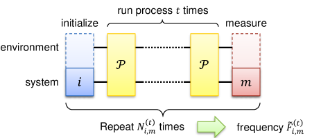
Figure 2: The experimental procedure for quantum process identification. An experiment consists of an initialization $i$, $t$ repetitions of the process, and a final YES/NO measurement $m$. Initializations and measurements nominally concern the system but are considered to involve the environment as well. Each experiment is repeated many times, yielding a frequency of YES outcomes. For the most complete and accurate results, all available initializations and measurements should be used, and the set of $t$ values should consist of widely spaced “flights” of consecutive values (see Section IV.1).

IV.2 Model Inference Procedure

Once the experiments are performed, the data is analyzed to infer a model of the process $\mathcal{P}$, the initial states, and the measurements. Our basic approach is to seek the model with the highest likelihood for the given observations. This is a challenging task for two reasons: (1) The size of the model (number of dimensions) is unknown. (2) The likelihood is extremely nonlinear in $T$: $T$ appears with powers up to $\max\mathcal{T}$, which in practice can be on the order of $10^{3}$ or more. This creates an extremely unforgiving optimization landscape with many local (and very suboptimal) maxima.

Regarding the first challenge, a number of techniques have been devised to compare the likelihood of models with different numbers of parameters (e.g. the Akaike information criterion Akaike (1974)) or to construct models whose complexity automatically scales with the complexity of the data (such as Dirichlet processes Buntine and Hutter (2010)). We use a simple but effective technique to first estimate the dimensionality of the process in question, which then determines the set of parameters to be estimated. The second challenge is essentially the same as that faced in gate set tomography. Building upon the progressive fitting approach described in Blume-Kohout et al. (2015), we devised a 4-stage model inference procedure, carefully honed over the course of our studies to reliably find concise, accurate process models. An overview of our procedure is given below; additional details are given in Appendices B-D.

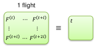
(a)

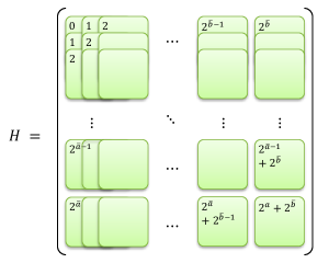
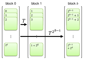
(b)	(c)

Figure 3: Arrangement of experimental data for analysis. (a) A flight is set of experiments with $2l+1$ consecutive values of process repetitions $t$, and is denoted by its lowest $t$ value. (b) For dimension estimation and initial model estimation, flights are arranged to form a large Ho-Kalman matrix. (c) Nonlinear model fitting is performed by grouping flights into blocks. The data in block $b$ is related to the data in block 0 by a factor of $T^{2^{b-1}}$, where $T$ is to be determined.

1. Estimate the Model Dimension. First, the data is arranged into a matrix $\tilde{H}$ which is the experimental estimate of the Ho-Kalman matrix $H$ (Fig. 3b). The effective dimension $d$ is estimated as the number of statistically significant non-zero singular values of $\tilde{H}$ Zeiger and McEwen (1974), where significance is assessed by a type of chi-squared test. In brief, the uncertainties in the experimental data are estimated and propagated to yield uncertainties in the singular values of $\tilde{H}$. This yields for each $k=0,1,2,\ldots$ a threshold for the sum of squares of the $k$ smallest singular values. If for some $k$ the sum falls below the threshold, those singular values are discounted (deemed insignificant). The dimension $d$ is taken to be the number of singular values that remain after the largest subset of singular values has been discounted. We note that this procedure does not determine the inherent dimension of a process so much as the dimension that is warranted by the data.

2. Obtain an Initial Model. This stage is a variation of the Ho-Kalman method, modified to account for uncertainty in the experimental data. Let $\tilde{H}^{\prime}$ be the “time shifted” version of $\tilde{H}$, i.e. the matrix obtained by increasing the $t$ value of each element of $\tilde{H}$ by 1. First, the variance of each experimental quantity $\tilde{F}_{i,m}^{(t)}$ is estimated. Then a rank-$d$ factorization $\tilde{H}\approx LR$ is found by minimizing $\sum_{i,m}W_{i,m}(LR-\tilde{H})_{i,m}^{2}$ where $W_{i,m}$ is the inverse variance of $\tilde{H}_{i,m}$. The process matrix is estimated as the matrix $T$ that minimizes $\sum_{i,m}W_{i,m}^{\prime}(LTR-\tilde{H}^{\prime})_{i,m}^{2}$ where $W_{i,m}^{\prime}$ is the inverse variance of $\tilde{H}_{i,m}^{\prime}$.

3. Obtain an Improved Model. Although the previous stage uses all the data, it uses only the fact that $\tilde{H}$ and $\tilde{H}^{\prime}$ are related by a (single) factor of $T$. It does not use the fact that data from different flights should be related by higher powers of $T$. To incorporate this relationship into the model estimate, the data is organized into groups of flights or “blocks” with exponentially increasing $t$ values (Fig. 3c). Starting with the matrices $L,T,R$ obtained in stage 2, a search is performed to find matrices $A,T,B$ that best fit the data in all the blocks, from which $S$ and $P$ are also extracted. To ensure that the search finds a good solution and does not get stuck in a local extremum, the search is performed progressively, starting with the lowest-$t$ blocks and gradually incorporating data from blocks with higher $t$ values. The low-$t$ blocks yield coarse estimates of $T$ which are gradually refined using the data in higher-$t$ blocks.

4. Obtain a physically valid model estimate. The model produced by stage 3 is usually fairly accurate, but tends to make slightly unphysical predictions (i.e., probabilities outside the interval $[0,1]$). In this last stage, the model likelihood is maximized with the addition of penalty terms to encourage the validity of predicted probabilities. As in stage 3, the log-likelihood is approximated by a weighted sum of squared errors; however, this time the weights are not based on the (fixed) experimental frequencies but are based on the predicted probabilities. Also, in this step the data is not arranged into Ho-Kalman matrices; the model (2) is fit directly to each experiment.

In our simulation studies, the model inference procedure described above proved to be both fast and reliable. In over 99% of the thousands of simulations we performed, it found a high-likelihood model without any intervention. In the few cases in which it did not, making minor adjustments to optimization parameters in stage 3 or 4 (e.g. penalty weights, convergence thresholds) invariably led to success. We found that all four stages were usually necessary to obtain accurate models. On a standard desktop computer, the time to complete all four stages ranged from just a few seconds for 7 dimensional processes to a few minutes for a 19-dimensional process.

V Simulations

To demonstrate the effectiveness of QPI, we simulated the characterization of several different non-Markovian processes relevant to quantum computing. Each process consists of a simple unitary operation on a qubit with a weak, physically-motivated non-Markovian error. In each case, the system of interest is the qubit and the non-Markovian behavior of the qubit is generated from a Markovian model of the qubit interacting with some external degree(s) of freedom. For these studies the error processes were chosen to be not only weak but also slow to reveal their non-Markovian nature, in order to present a strong characterization challenge.

For each process, we first simulated the evolution of the quantum state for several different initial states and predicted the time-dependent outcome probabilities for the standard tomographic measurements. The “standard tomographic measurements” are the measurements of the dimensionless Pauli operators $\sigma_{x},\sigma_{y},\sigma_{z}$. These operators have eigenvalues $+1$ (“YES”) and $-1$ (“ NO”) with corresponding eigenstates denoted $|\pm\rangle_{x}$,$|\pm\rangle_{y}$,$|\pm\rangle_{z}$, respectively. For simplicity, state preparation and measurement were assumed to be ideal. Then, we simulated the collection of experimental data by choosing a random number of YES outcomes for each measurement from the computed probability distribution. The simulated data for each experiment was then passed to our data analysis code, which estimated the dimension of the process and found the most likely model using the procedure outlined above. The error of the characterization was calculated by using the inferred model to predict the time-dependent qubit state and comparing the predicted state to the true (simulated) state. The error at each time step was averaged over all initial states and over 500 independent simulated characterizations (200 for the system described in section V.4).

In each plot below, black dots show the times of the (simulated) measurements and their average error, where error is defined as the trace distance $\frac{1}{2}\operatorname{Tr}\left|\rho(t)-\rho_{\text{est}}(t)\right|$ between the true state $\rho(t)$ and the state $\rho_{\text{est}}(t)$ estimated from the measurements at time $t$ only. The blue line is the QPI error, defined as the average trace distance between the true state $\rho(t)$ and the state $\rho_{\text{QPI}}(t)$ predicted by QPI, which is based on all the simulated measurements. For comparison, the dotted black line is the corresponding error for perfect quantum process tomography, obtained using the exact measurement probabilities at $t=0$ and $t=1$ only.

V.1 Qubit Rotation with Slowly Varying Systematic Error

In quantum computing technologies, operations on qubits are typically accomplished by applying control pulses that temporarily modify the Hamiltonian to induce a unitary rotation of one or more qubits. In many implementations the amount of rotation is proportional to the pulse energy. A miscalibration of the pulse intensity or duration results in over- or under-rotation of the qubits, which generally contributes to computational error Barnes et al. (2017).

In this example the process of interest is an intended $\pi$ rotation of a qubit about the $y$ axis, i.e. a bit flip. We suppose however that the intensity of the control pulse drifts sinusoidally over time, such that the actual angle of rotation produced by the pulse at time $t$ (where each pulse takes one unit of time) is

$$\theta_{t} =\pi+\epsilon\sin\Omega t.$$ (20)

We choose $\epsilon=0.01$ and $\Omega=0.02$, which yields a small, slow oscillation of the qubit about the intended state in the $x$-$z$ plane. This oscillation cannot be described by any fixed Markovian process involving only the qubit. In fact, the error can be described as phase modulation, a process which has an infinite number of sidebands. In other words, this process technically has an infinite dimension. However, relatively few dimensions are needed to accurately reproduce typical experimental data.

The evolution of the qubit under this process was simulated for two different initial states, $|+\rangle_{z}$ and $|+\rangle_{x}$. For each initial state, tomographic measurements of the qubit were simulated at 304 times ranging from $t=0$ to $t=1035$, forming 57 flights of length 12. Each measurement was repeated $10^{4}$ times. In nearly all realizations, model inference yielded an 11-dimensional model. Fig. 4 shows the average characterization error as a function of $t$.

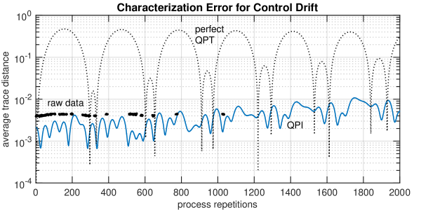
Figure 4: Average characterization error (solid line) for a qubit undergoing $\pi$ rotations with small, sinusoidally varying error in the rotation angle. Also shown for comparison are the raw measurement error (dots) and error of perfect process tomography (dotted line).

V.2 Coherent Qubit Leakage

Leakage refers to the loss of a qubit, or more precisely, the transition of a qubit to a non-computational state. This process is usually modeled as irreversible and incoherent, in which case the qubit has no effect on any subsequent operation. More realistically, qubit operations create and manipulate superpositions of computational and non-computational states Wood and Gambetta (2017). In such cases a qubit can effectively leave and later return to the computational subspace, interfering with the computational evolution. The particular details of the qubit’s behavior will depend strongly on the physics of the physical implementation of the qubit and the control mechanisms employed. For this example we use the 3-level anharmonic oscillator model which is applicable to popular qubit technologies including superconducting flux qubits and trapped ions Gambetta et al. (2011). In this model, the control pulse drives not only the intended $|0\rangle\leftrightarrow|1\rangle$ transition, but also off-resonant transitions between $|1\rangle$ and the next excited state $|2\rangle$. The interaction Hamiltonian is

$$H =\Omega(t)\left(|0\rangle\langle 1|+\sqrt{2}|1\rangle\langle 2|+\text{H.c}\right)+\Delta|2\rangle\langle 2|$$ (21)

where $\Omega(t)$ is the control amplitude and $\Delta$ is the detuning of the non-computational state. For simulations we used Gaussian control pulses of width 0.25 time steps (truncated to have 1 time step duration) and chose an excited state detuning $\Delta=20$ yielding a system in which the leakage in and out of the computational space is small but not negligible. For these parameter values the total probability of state $|2\rangle$ oscillates with a period of nearly 30 time steps, with maximal value of a few percent. Meanwhile, the computational state slowly precesses about the intended state.

The evolution of this 3-level system was simulated for four different initial qubit states ($|+\rangle_{z}=|0\rangle$, $|-\rangle_{z}=|1\rangle$, $|+\rangle_{x}$, and $|+\rangle_{y}$). For each initial state, tomographic measurements of the qubit were simulated at 196 times ranging from $t=0$ to $t=1029$, forming 57 flights of length 6. Each measurement was repeated $10^{4}$ times. In nearly all cases, the model inference yielded a 7-dimensional model. The average characterization error for this process is shown in Fig. 5.

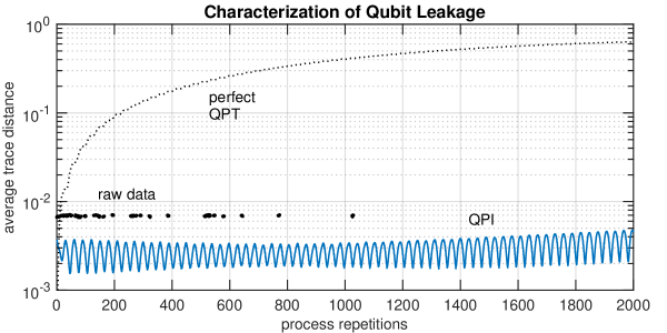
Figure 5: Average characterization error (solid line) for a qubit undergoing bit flips in the anharmonic oscillator model. Also shown for comparison are the raw measurement error (dots) and error of perfect process tomography (dotted line).

V.3 A Qubit Coupled to a Single Impurity

Another potential source of error in qubit devices is unintended coupling between qubits, or between a qubit and a nearby impurity. A simple model for such coupling is the isotropic spin exchange Hamiltonian

$$H =\gamma\left(\sigma_{x}\otimes\sigma_{x}+\sigma_{y}\otimes\sigma_{y}+\sigma_{z}\otimes\sigma_{z}\right).$$ (22)

Taking $\gamma=0.01$ to model weak coupling, the evolution of a qubit and impurity spin was simulated for three initial qubit states ($|+\rangle_{x}$, $|+\rangle_{y}$, and $|+\rangle_{z}$). The impurity is always initially in the state $|+\rangle_{z}$. For each initial state, tomographic measurements were simulated at 64 times ranging from $t=0$ to $t=1030$, forming 12 flights of length 7. Each measurement was repeated $10^{4}$ times. In nearly all cases, model inference yielded a 7-dimensional model. This may be compared with the nominal dimension $4^{2}=16$ of a two qubit system. The average characterization error for this process is shown in Fig. 6.

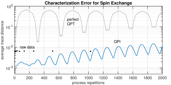
Figure 6: Average characterization error (solid line) for a qubit weakly coupled to an impurity via a spin-exchange interaction. Also shown for comparison are the raw measurement error (dots) and error of perfect process tomography (dotted line).

V.4 ³¹P Qubit in Silicon

For our final case study, we considered a ${}^{31}\text{P}$ donor in ${}^{28}\text{Si}$ with ${}^{29}\text{Si}$ impurities. The nuclear spin of the ${}^{31}\text{P}$ defines a qubit. The qubit is manipulated by a time-varying magnetic field which also affects the impurities. Meanwhile, the ${}^{31}\text{P}$ and ${}^{29}\text{Si}$ impurities interact via hyperfine coupling to the donor electron. A detailed model for this system was formulated in Lougovski and Peters (2017). We simulated the behavior of the qubit and impurities in response to a sequence of pulses that each nominally produce a $\pi$ rotation of the qubit (bit flip). For these simulations, the donor was imagined to be at the center of a $(5\thinspace\text{nm})^{3}$ cube with a ${}^{29}\text{Si}$ concentration of 800 ppm, which translates to 6 impurities in the qubit volume. The impurities were distributed randomly throughout the volume; in all, 200 random configurations were simulated. The background magnetic field $B_{z}$ was 1.5 T, the amplitude $B_{x}$ of the driving magnetic field was 0.15 T, and the ambient temperature was 250 mK. (For further details see Lougovski and Peters (2017)).

For each configuration of the impurities, the evolution of the donor and impurities was simulated for 4 different initial qubit states ($|+\rangle_{x}$,$|+\rangle_{y}$,$|+\rangle_{z}$, and $|-\rangle_{z}$) and with the impurities initially in thermal equilibrium. For each initial state, tomographic measurements of the qubit were simulated at 272 different time steps ranging from $t=0$ to $t=1033$, forming 57 flights of length 10. Each measurement was repeated $10^{3}$ times. In most realizations the inferred model dimension was 19 or 20, which is much less than the nominal dimension of the ${}^{31}\mathrm{P}+^{29}\mathrm{Si}$ system (7 nuclear spins + 1 electron spin = 8 spins with a nominal dimension of $(2^{8})^{2}=65,536$). Thus QPI reveals that the effective interaction between the qubit and the impurities involves only a small subspace of the available Hilbert space, an insight that is not readily apparent from the underlying model. The average characterization error for this system is shown in Fig. 7

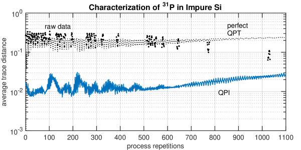
Figure 7: Average characterization error (solid line) for a ³¹P donor qubit with 6 nearby ²⁹Si impurities. Also shown for comparison are the raw measurement error (dots) and error of perfect process tomography (dotted line).

VI Discussion

In all of the simulation studies above, our QPI method was able to accurately capture and reproduce the observable behavior of the qubit over very long time scales, with trace distance errors on the order of $10^{-2}$. While this level of error would not be impressive for tomography of the state at any one time, the fact that this accuracy is maintained over more than a thousand time steps implies that the process itself is actually characterized to an accuracy on the order of $10^{-5}$. Notably, the inferred models remained accurate well beyond the times at which measurements were taken (although the errors did tend to slowly grow the farther in time the models were extrapolated).

In contrast, standard quantum process tomography (which uses measurements only at $t=0$ and $t=1$) yielded inaccurate predictions of qubit behavior past a few tens of time steps, even under the assumption of zero statistical measurement error. Arguably, it would be fairer to compare QPI with a version of QPT that incorporates the data at all times, but assumes the process is Markovian. This can be achieved in our framework by restricting the model dimension to 4 for characterization of a single qubit. In fact we attempted to perform such a comparison, but found that dimension-limited (Markovian) models were such a poor fit to the data that the model inference would not converge.

For the finite dimensional processes studied (leakage and spin exchange), QPI inferred a process dimension that was equal to or close to the true dimension. For the high-dimensional processes studied (control drift and ${}^{31}\mathrm{P}+^{29}\mathrm{Si}$ systems), QPI was able to reproduce the observed behavior using relatively low-dimensional models. Fortunately, it was not necessary to use flights as long as suggested by the worst-case bound of Lemma 1.

Although these simulation studies addressed processes nominally involving a single qubit, QPI is in principle just as applicable to the characterization of qudit or multiqubit operations. However, the state space size (and hence also the cost of data collection and data analysis) grows exponentially with the number of qubits. Thus like all forms of tomography, QPI is really only feasible for characterizing small quantum systems. Indeed, a possible concern is that QPI appears to require much more experimental data than QPT, which already requires a moderately large amount of data. To some extent this is to be expected: whereas QPT needs only enough information to produce a 4-dimensional model for a qubit process, QPI needs enough information to first of all determine the effective size of the environment’s memory and then determine all the dynamical parameters involving the qubit, the pertinent part of the environment, and their interaction. We expect, however, that QPI can be made much more efficient than the studies above would suggest. In these studies, all measurements were arbitrarily chosen to be performed the same number of times. Almost certainly some measurements are more informative than others. We expect that an adaptive testing strategy, in which the current model estimate is used to choose the most informative experiment to perform next, will significantly reduce the cost of QPI Huszár and Houlsby (2012); Mahler et al. (2013); Granade et al. (2015).

As presented here, QPI has two main limitations. The first is that it characterizes only one process. In the context of a quantum computer, one would like a self-consistent characterization of all qubit operations (“gates”) that may be performed; under the assumption of Markovianity, GST provides just such a characterization. As formulated here, QPI would yield a set of separate characterizations, one for each gate, that cannot be related. More specifically, the relationship between latent variables in the models for different gates would be indeterminate, i.e. one would not know whether different gates interact with the same or different environmental degrees of freedom. We conjecture that QPI can be extended to jointly characterize a set of processes: The principles of the Ho-Kalman method extend in a straightforward way to this case. What is unclear at present is how to extend Lemma 1, i.e. how to identify a relatively small set of operation sequences that are likely to yield a complete model. This is an obvious direction for future work.

In principle, extending QPI to multiple processes would allow cross talk and other spatial correlations to be characterized by treating different combinations of simultaneous gates as different processes. However, due to the very large number of different combinations this would constitute (even in a small device), this does not seem to be a practical approach to characterizing spatial correlations.

The other main limitation of QPI as described here is that it assumes all measurements are final; no attempt is made to model the effect of the measurement on the state of the system or environment. But intermediate measurements are a key component of quantum error correction protocols, thus the ability to characterize their impact on the remainder of a computation is important. We suspect the ability to characterize intermediate measurements would follow from the ability to characterize multiple processes, since each outcome of a measurement can be treated as a distinct, randomly selected process.

VII Conclusion

In conclusion, we have developed a new method for the characterization of quantum dynamical processes, called quantum process identification. QPI goes beyond state-of-the-art methods by providing the means to systematically characterize non-Markovian dynamics as well as Markovian dynamics. We presented a detailed experimental protocol and data analysis procedure and demonstrated their effectiveness using numerical simulations of realistic non-Markovian error processes affecting qubits. Directions for future work include extending QPI to enable the characterization of multiple processes and non-final measurements, and using adaptive strategies to reduce its experimental cost. Apart from experimental applications, the theory underlying QPI elucidates the relationship between the temporal evolution of an open quantum system and its effective environment, providing a useful alternative to existing representations of non-Markovian quantum dynamics.

This research was sponsored by the Laboratory Directed Research and Development Program of Oak Ridge National Laboratory, managed by UT-Battelle, LLC, for the U. S. Department of Energy. The authors would like to express appreciation to Nicholas Peters for helpful comments on the preparation of this manuscript.

Appendix A Proof of Lemma 1

In this section we show that the minimum number of time observations needed to guarantee complete characterization of a discrete-time linear system depends on the number of latent (unmeasured) degrees of freedom, not the total number of degrees of freedom. Let $d$ be the true dimension of the system and let $a$ be the dimension of the subspace spanned by the initial states and measured quantities. We show that $\operatorname{rank}(H_{l+1})=d$ where $l=d-a$ and $H_{l}$ is the block-Hankel matrix formed from $X(1),\ldots,X(2l-1)$. It follows from the Ho-Kalman theory that $X(1),\ldots,X(2(l+1))$ are sufficient to obtain a state model of the system .

The goal is to find matrices $L,M,R$ such that $X(k)=LM^{k-1}R$. In the remainder of this section, $X(k)$ will be denoted more compactly as $X_{k}$. For convenience, we assume that redundant initial states and redundant measurements have been omitted, so that $X(k)$ is $a\times a$. Since $\operatorname{rank}X_{i}\leq a$ for every $X_{i}$, we may choose a representation in which $L$ has the form $L=\left[\begin{array}[]{cc}1_{a\times a}&0_{a\times l}\end{array}\right]$. It follows that $R=\left[\begin{array}[]{c}X_{0}\\ Y_{0}\end{array}\right]$ where $Y_{0}$ is some unknown $l\times a$ matrix. We write $M$ as

$$M \equiv\left[\begin{array}[]{cc}A&B\\ C&D\end{array}\right]$$ (25)

where $A$ is $a\times a$, $D$ is $l\times l$, and $B$ and $C$ are sized correspondingly. We have

$$\left[\begin{array}[]{c}X_{n}\\ Y_{n}\end{array}\right] \equiv M^{n}\left[\begin{array}[]{c}X_{0}\\ Y_{0}\end{array}\right]$$ (30)

$$=\left[\begin{array}[]{cc}A&B\\ C&D\end{array}\right]\left[\begin{array}[]{c}X_{n-1}\\ Y_{n-1}\end{array}\right].$$ (35)

Then

$$X_{n+1} =AX_{n}+BY_{n}$$ (36)

$$=AX_{n}+B(CX_{n-1}+DY_{n-1})$$ (37)

$$\vdots$$ (38)

$$=AX_{n}+\left(\sum_{i=1}^{k}BD^{i-1}CX_{n-i}\right)+BD^{k}Y_{n-k}$$ (39)

or

$$X_{n+k+1}=AX_{n+k}+\left(\sum_{i=1}^{k}BD^{i-1}CX_{n+l-i}\right)+BD^{k}Y_{n}$$ (40)

for $k=0,1,2,\ldots,n$. Let $k=l$. Our goal is to eliminate $Y_{n}$ and obtain a recurrence relation involving only the $X_{j}$’s. By the Cayley-Hamilton theorem there are coefficients $\alpha_{0},\ldots,\alpha_{l-1}$ such that $D^{l}=\sum_{j=0}^{l-1}\alpha_{i}D^{i}$. Thus

$$X_{n+l+1}=AX_{n+l}+\left(\sum_{i=1}^{l}BD^{i-1}CX_{n+l-i}\right)+\sum_{j=0}^{l-1}\alpha_{j}BD^{j}Y_{n}.$$ (41)

Setting $k$ to $j$ in (40) yields

$$X_{n+j+1} =AX_{n+j}+\left(\sum_{i=1}^{j}BD^{i-1}CX_{n+j-i}\right)+BD^{j}Y_{n}.$$ (42)

Solving for $BD^{j}Y_{n}$ and substituting into (41) gives

$$X_{n+l+1} =AX_{n+l}+\left(\sum_{i=1}^{l}BD^{i-1}CX_{n+l-i}\right)+\sum_{j=0}^{l-1}\alpha_{j}\left(X_{n+j+1}-AX_{n+j}-\sum_{i=1}^{j}BD^{i-1}CX_{n+l-i}\right)$$ (43)

$$=AX_{n+l}+\sum_{i=1}^{l}\left(1-\sum_{j=i}^{l-1}\alpha_{j}\right)BD^{i-1}CX_{n+l-i}+\sum_{j=0}^{l-1}\alpha_{j}\left(X_{n+j+1}-AX_{n+j}\right)$$ (44)

The important thing to note about this last equation is that $X_{n+l+1}$ is written in terms of $X_{n},\ldots,X_{n+l}$. More precisely, there are matrices $Q_{0},\ldots,Q_{l}$ such that

$$X_{n+l+1}=\sum_{i=0}^{l}Q_{i}X_{n+i}.$$ (45)

In other words, the rows of $X_{n+l+1}$ are linear combinations of the rows of $X_{n},\ldots,X_{n+l}$. (Note that if the $Q_{i}$’s were scalars instead of matrices, the effective dimension of the system would be at most $l+1$.) By extension,

$$\mathcal{T}_{n+l+1} =\sum_{i=0}^{l}Q_{i}\mathcal{T}_{n+i}$$ (46)

where $\mathcal{T}_{k}\equiv\left[\begin{array}[]{ccc}X_{k}&X_{k+1}&\cdots\end{array}\right]$ is the $k$th block of rows of $H_{\infty}$. Thus $\mathcal{T}_{1},\ldots,\mathcal{T}_{l+1}$ span $\mathcal{T}_{l+1}$ and, by induction, all rows of $H_{\infty}$.

Now, we could just as well have chosen a representation in which $R=[\begin{array}[]{cc}1_{a\times a};&0\end{array}]$ and $L=\left[\begin{array}[]{cc}X_{0}&Z_{0}\end{array}\right]$, and written

$$\left[\begin{array}[]{c}X_{n}\\ Z_{n}\end{array}\right]=\left[\begin{array}[]{c}X_{0}\\ Z_{0}\end{array}\right]M^{n}=\left[\begin{array}[]{c}X_{n-1}\\ Z_{n-1}\end{array}\right]\left[\begin{array}[]{cc}A&B\\ C&D\end{array}\right].$$ (55)

This is the same problem as above, except that $Y_{n}$ is replaced by $Z_{n}$, $B$ and $C$ swap roles, and recurrence relations involve factors of $A,B,C,D$ on the right rather than on the left. A derivation analogous to that above would show that there exist matrices $Q_{0}^{\prime},\ldots,Q_{l}^{\prime}$ such that

$$X_{n+l+1} =\sum_{i=0}^{l}X_{n+i}Q_{i}^{\prime}$$ (56)

by which we conclude that the first $a(l+1)$ columns span all the columns of $H_{\infty}$. Thus $\operatorname{rank}(H_{l+1})=\operatorname{rank}(H_{\infty})=a+l$. It follows from the Ho-Kalman theory that $X_{1},\ldots,X_{2(l+1)}$ are sufficient to determine any system of dimension up to $a+l$.

Conversely, observing the output at less than $2(l+1)$ times is generally insufficient to reproduce the system’s behavior. We omit a detailed proof, but note that this fact can be established by constructing a $d$-dimensional system with a size $l$ shift register that does not reveal its presence until the $(l+1)$th time step. For this process $\operatorname{rank}H_{l}<\operatorname{rank}H_{l+1}=d$. Similarly, it is easy to show that observing the output at non-consecutive times is also generally insufficient to construct a correct model. Consider a scalar system whose impulse response function (starting at time $t=0$) cycles through the values $\alpha\to\beta\to\alpha\to\gamma\to\ldots$. If the outputs are observed only at $t=0,1,2,4,\ldots,2^{k},\ldots,$ the value $\gamma$ would never be observed and a two-state system with output $\alpha\rightarrow\beta\rightarrow\alpha\rightarrow\beta\rightarrow\cdots$ would be inferred.

Appendix B Dimension Estimation

In this section we consider the problem of estimating the dimension $d$ of a process from an experimental estimate $\tilde{H}$ of a Ho-Kalman matrix $H$. Ho and Kalman showed if $H$ is sufficiently large, then $d$ is just the rank of $H$. But $\tilde{H}$, which is a random perturbation of $H$, has a rank that is generally much higher than $d$. The singular values of $\tilde{H}$ are much more informative than the rank, as they reveal the magnitude of each dimension’s contribution to the data. If the statistical errors in the data are small, all but $d$ singular values of $\tilde{H}$ will be small. Here we derive a reliable criterion for determining which singular values are small enough to be considered spurious.

A naive approach would be to set a threshold for each singular value—say, based on its estimated variance—and count the number of singular values that exceed their threshold. There are problems with this approach, however, the most serious being that the number of singular values that exceed their threshold simply by chance grows with the size of $\tilde{H}$, i.e. grows with the number of experiments performed. A way to overcome this problem is to test singular values collectively rather than individually: Given a threshold for statistical significance of the $k$ smallest singular values, one finds the largest $k$ for which the threshold is not met and takes $d$ to be the number of singular values that remain.

An appropriate threshold can be derived from the uncertainty in the raw data. Each quantity $\tilde{F}_{i,m}^{(t)}$ that appears in $\tilde{H}$ is an independent random variable, distributed binomially with mean $F_{i,m}^{(t)}$ and variance $F_{i,m}^{(t)}(1-F_{i,m}^{(t)})/N_{i,m}^{(t)}$. Let $\epsilon_{i,t,m}=\tilde{F}_{i,m}^{(t)}-F_{i,m}^{(t)}$ denote the statistical deviation of $\tilde{F}_{i,m}^{(t)}$ and let $\partial_{(i,t,m)}H\equiv\partial H/\partial F_{i,m}^{(t)}$. Then

$$\tilde{H} =H+\sum_{x}(\partial_{x}H)\epsilon_{x}$$ (57)

where $x$ ranges over all experiments $(i,t,m)$. Let $h_{1}\times h_{2}$ be the size of $H$ and let $h=\min(h_{1},h_{2})$. Let $H=USV^{\dagger}$ be a “full” singular value decomposition of $H$, i.e. $U$ is $h_{1}\times h_{1}$ and $V$ is $h_{2}\times h_{2}$, and $S$ is $h_{1}\times h_{2}$ with diagonal elements $s_{1}\geq s_{2}\geq\cdots\geq s_{h}$. Let $U_{k}$ be the matrix consisting of columns $k$ through $h_{1}$ of $U$, and $V_{k}$ the matrix consisting of columns $k$ through $h_{2}$ of $V$.

Suppose $H$ has rank $r$. Then $s_{1},\ldots,s_{r}\neq 0$ and $s_{r+1}=\cdots=s_{h}=0$. According to perturbation theory, the corresponding singular values $\tilde{s}_{r+1},\ldots,\tilde{s}_{h}$ of $\tilde{H}$ are the singular values of

$$A \equiv U_{r+1}^{\dagger}\tilde{H}V_{r+1}$$ (58)

$$=U_{r+1}^{\dagger}\left(H+\sum_{x}(\partial_{x}H)\epsilon_{x}\right)V_{r+1}.$$ (59)

Since $U_{r+1}^{\dagger}HV_{r+1}=0$ we have

$$A =\sum_{x}A_{x}\epsilon_{x}$$ (60)

where

$$A_{x} \equiv U_{r+1}^{\dagger}(\partial_{x}H)V_{r+1}.$$ (61)

Let $\chi_{r}$ denote the residual “energy” of the $h-r$ smallest singular values,

$$\chi_{r} =\sum_{i>r}\tilde{s}_{i}^{2}$$ (62)

$$=\operatorname{Tr}(A^{T}A)$$ (63)

$$=\sum_{x,y}\operatorname{Tr}(A_{x}^{T}A_{y})\epsilon_{x}\epsilon_{y}.$$ (64)

Owing to the independence of experiments, we have $\left<\epsilon_{x}\epsilon_{y}\right>=0$ for $x\neq y$, yielding

$$\left<\chi_{r}\right> =\sum_{i,j>r}\sum_{x}B_{ij}^{(x)}$$

where $B^{(x)}\equiv A_{x}\sqrt{\left<\epsilon_{x}^{2}\right>}$.

If the threshold for rejecting $\tilde{s}_{r},\ldots,\tilde{s}_{h}$ were set at $\left<\chi_{r}\right>$, then approximately half of the time the subset $\tilde{s}_{d+1},\ldots,\tilde{s}_{h}$ would be incorrectly accepted as statistically significant, resulting in an overestimate of $d$. A higher threshold reduces the probability of this occurring, but increases the probability of rejecting $\tilde{s}_{d},\ldots,\tilde{s}_{h}$ and thereby underestimating $d$. Thus the threshold should be just high enough to reject $\tilde{s}_{d+1},\ldots,\tilde{s}_{h}$ a majority of the time. To that end we calculate the variance of $\chi_{r}$. We have

$$\chi_{r}^{2} =\operatorname{Tr}(A^{T}A)^{2}$$

$$=\sum_{x,y}\sum_{p,q}\operatorname{Tr}(A_{x}^{T}A_{y})\operatorname{Tr}(A_{p}^{T}A_{q})\epsilon_{x}\epsilon_{y}\epsilon_{p}\epsilon_{q}.$$

Since the deviations are independent and zero-mean, $\left<\epsilon_{x}\epsilon_{y}\epsilon_{p}\epsilon_{q}\right>$ vanishes unless it is of the form $\left<\epsilon_{x}^{4}\right>$ or $\left<\epsilon_{x}^{2}\epsilon_{y}^{2}\right>$. The second form simplifies to $\left<\epsilon_{x}^{2}\right>\left<\epsilon_{y}^{2}\right>$. Provided the statistical errors are small compared to the quantities being estimated, $\epsilon_{x}$ has an approximately normal distribution, for which $\left<\epsilon_{x}^{4}\right>=3\left<\epsilon_{x}^{2}\right>^{2}$. Then

$$\left<\chi_{r}^{2}\right> =3\sum_{x}\operatorname{Tr}(A_{x}^{T}A_{x})^{2}\left<\epsilon_{x}^{2}\right>^{2}+\sum_{x}\sum_{y\neq x}\left(\operatorname{Tr}(A_{x}^{T}A_{x})\operatorname{Tr}(A_{y}^{T}A_{y})+2\operatorname{Tr}(A_{x}^{T}A_{y})^{2}\right)\left<\epsilon_{x}^{2}\right>\left<\epsilon_{y}^{2}\right>$$

$$=\left(\sum_{x}\operatorname{Tr}(A_{x}^{T}A_{x})\left<\epsilon_{x}^{2}\right>\right)^{2}+2\sum_{x,y}\operatorname{Tr}(A_{x}^{T}A_{y})^{2}\left<\epsilon_{x}^{2}\right>\left<\epsilon_{y}^{2}\right>$$

$$=\left<\chi_{r}\right>^{2}+2\sum_{i,j>r}\sum_{k,l>r}\left(\sum_{x}B_{ij}^{(x)}B_{kl}^{(x)}\right)^{2}$$ (65)

where

$$D_{i,j;k,l} \equiv\sum_{x}B_{ij}^{(x)}B_{kl}^{(x)}.$$ (66)

Our criterion for accepting the hypothesis $s_{r+1}=s_{r+2}=\cdots=0$ is

$$\chi_{r} \leq\left<\chi_{r}\right>+\sqrt{\operatorname{Var}\chi_{r}}$$ (67)

$$=\sum_{i,j>r}\sum_{x}B_{i,j}^{(x)}+\sqrt{2\sum_{i,j>r}\sum_{k,l>r}\left(\sum_{x}B_{ij}^{(x)}B_{kl}^{(x)}\right)^{2}}.$$ (68)

We take $d$ be the smallest $r$ for which this criterion is met. In theory the probability of overestimating $d$ is then at most 0.16.

In practice this criterion cannot be applied exactly: The quantities on the right side of eq. (68) are not known, but can only be estimated. The singular values may not even be in quite the right order due to statistical variations. Furthermore, the approximations made in the derivation might not always be accurate. Nevertheless, in our simulations we observed that the criterion (68) is effective: It usually yields an estimate of $d$ quite close to the true value, provided one has taken enough data.

Appendix C Progressive Fitting of Data Blocks

For large times $t$, the experimental quantity $F^{(t)}=ST^{t}P$ is an extremely nonlinear function of $T$, presenting a considerable challenge for estimation of the parameters $S,T,P$ from the data. Building on the approach described in Blume-Kohout et al. (2015), we devised a progressive fitting method which first uses low-$t$ data to obtain a coarse estimate of $T$, then gradually incorporates data with higher $t$ to increase the accuracy of the model. Our implementation involves multiple passes over the data, alternating between optimization of $T$ given the current estimate of $S,P$ and optimization of $S,P$ given the current estimate of $T$. We found that if too much or too little data was used at any given step, either $(S,P)$ or $T$ could “lock in” to the wrong region of parameter space from which the search could not recover. The procedure below was carefully honed to ensure that at each step, only reliable intermediate estimates were used. In our studies, 5-15 passes were usually sufficient to obtain good fits to the data.

Let $H^{(b)}$ denote the $b$th block of data (Fig. 3c), $W^{(b)}$ the matrix of corresponding statistical weights, and $N_{b}$ the number of elements in these blocks. (The weights $W^{(b)}$ are adjusted to account for the different multiplicity of different experiments, so that each experiment has the same total weight.) The function to be minimized is

$$\Phi_{b}(A,T,B) \equiv\frac{1}{N_{b}}\sum_{b^{\prime}=0}^{b}\sum_{i\in\mathcal{I}}\sum_{m\in\mathcal{M}}W_{i,m}^{(b^{\prime})}(AT^{\varrho_{b^{\prime}}}B-H^{(b^{\prime})})_{i,m}^{2}$$ (69)

which is the average weighted error of the model over blocks $0$ through $b$. Under the true model, the distribution of $\Phi_{b}$ has a strong peak at 1. A value significantly larger than this (say, 1.5) indicates a poor fit. Model fitting with the correct dimension usually yields $\Phi_{b}$ values around 0.8; overfitting leads to $\Phi_{b}$ around 0.5.

Recall that $\bar{b}$ is the index of the last block. Let $b_{\text{highest}}$ denote the index of the highest block for which a fit has been attempted. The fitting procedure is as follows:

1. Let $(L,T,R)$ be the outputs of Ho-Kalman estimation. Set $A$ equal to $L$ and set $B$ equal to the first $n(l+1)$ columns of $R$. Find the smallest $b$ such that $\Phi_{b}>1.5$ and set $b_{\text{highest}}$ to this value (or to $\bar{b}$ if there is no such $b$.)

2. Keeping $T$ fixed, optimize $A,B$. This is accomplished by minimizing a modified form of eq. (69) with $b=\bar{b}$. Whereas the current estimate of $T$ is used for blocks $b^{\prime}\leq b_{\text{highest}}$, for blocks $b^{\prime}>b_{\text{highest}}$ we replace $T^{\varrho_{b^{\prime}}}$ by the matrix $Y^{(b^{\prime})}$ that is optimal with respect to $A,B$. In this way $A,B$ are made to fit all the data but are not constrained by high powers of $T$ that have not yet been determined to be accurate. Minimization can be accomplished via iterative linear algebraic methods.

3. Keeping $A,B$ as fixed, optimize $T$.

   1. Set $b=2$.

   2. If $b<b_{\text{highest}}$ and $\Phi_{b}\leq 1.5$, continue to 3.3.3. Otherwise, find $T$ that minimizes $\Phi_{b}$, keeping $A,B$ fixed. This can be accomplished by various nonlinear optimization methods; we found the Gauss-Newton method with line search to work well.

   3. If $b<\bar{b}$ and $\Phi_{b}\leq 1.5$, increase $b$ by 1, set $b_{\text{highest }}=\max(b,b_{\text{highest}})$, and go back to 3.3.2.

4. If $b=\bar{b}$ and $\Phi_{\bar{b}}$ did not improve significantly (say, by more than 0.001) compared to the previous pass, optimization has converged; continue to step 3.5. Otherwise, go back to step 3.2 (perform another pass).

5. If $\Phi_{\bar{b}}\leq 1.5$, the fit is deemed a success; in this case return $T$, return the first $m$ rows of $A$ for $S$, and return the first $n$ columns of $B$ for $P$. Otherwise, increase $d$ by one, perform Ho-Kalman estimation again (stage 2, described in Section IV.2), and start again at step 3.1.

Appendix D Final Model Optimization

The fourth and final stage of our model inference procedure is to fit the model $F^{(t)}=ST^{t}P$ directly to the data. This last stage yields the most accurate models but requires a very good starting estimate $S,T,P$. As in the previous stage, we minimize a sum of weighted squared errors. But unlike in previous stages, the weights are determined by the model itself rather than estimated from the data, making the total squared error a good proxy for the negative log likelihood. Besides being simpler to work with than the log likelihood, weighted errors allow out-of-range probabilities (less than 0 or grater than 1) to be handled much more gracefully. In this stage we also impose soft constraints on the eigenvalues $\{\lambda_{i}\}$ of $T$: Since the process in question is presumed to occur in a finite state space, the eigenvalues of $T$ should not have magnitude greater than 1, as otherwise repeated application of the process would eventually take the state out of the state space.

The function to be minimized is

$$\Psi(S,T,P) \equiv\frac{1}{\left|\mathcal{I}\right|\left|\mathcal{M}\right|\left|\mathcal{T}\right|}\sum_{t\in\mathcal{T}}\sum_{i\in\mathcal{I}}\sum_{m\in\mathcal{M}}W_{i,m}^{(t)}\left(S,T,P\right)\left(F^{(t)}-\tilde{F}^{(t)}\right)_{i,m}^{2}+E(T).$$ (70)

where $E(T)=\sum_{i}\max(0,\left|\lambda_{i}\right|-1)^{2}$ is the eigenvalue constraint. Nominally, $W_{i,m}^{(t)}$ is the inverse variance of $F_{i,m}^{(t)}$. But since the inverse variance becomes negative or infinite if the model ever predicts $F_{i,m}^{(t)}\leq 0$ or $F_{i,m}^{(t)}\geq 1$, we take

$$W_{i,m}^{(t)} =\frac{1}{V_{i,m}^{(t)}+\sqrt{V_{i,m}^{(t)2}+4\beta_{i,m}^{(t)2}}}$$ (71)

where

$$V_{i,m}^{(t)} =\frac{F_{i,m}^{(t)}(1-F_{i,m}^{(t)})}{N_{i,m}^{(t)}}$$ (72)

is the theoretical variance of $F_{i,m}^{(t)}$ and $\beta_{i,m}^{(t)}$ is a small buffer term that ensures $W_{i,m}^{(t)}$ remains finite, continuous, and positive. We start with $\beta_{i,m}^{(t)}=1/N_{i,m}^{(t)}$. We then proceed to minimize 70 using the Gauss-Newton method with line search. After each search step the validity of the model predictions are assessed. If any $F_{i,m}^{(t)}$ is not in the interval $[0,1]$, $\beta_{i,m}^{(t)}$ is reduced by 5%. This increases $W_{i,m}^{(t)}$ outside $[0,1]$ and near its endpoints, thereby more strongly encouraging $F_{i,m}^{(t)}$ to become valid. If after a search step all the predicted probabilities are valid and $\Psi$ was not significantly improved, the search concludes.

References

- Scarani et al. (2009) V. Scarani, H. Bechmann-Pasquinucci, N. J. Cerf, M. Dušek, N. Lütkenhaus, and M. Peev, Reviews of Modern Physics 81, 1301 (2009).
- Kelly et al. (2014) J. Kelly, R. Barends, B. Campbell, Y. Chen, Z. Chen, B. Chiaro, A. Dunsworth, A. G. Fowler, I.-C. Hoi, E. Jeffrey, A. Megrant, J. Mutus, C. Neill, P. J. J. O’Malley, C. Quintana, P. Roushan, D. Sank, A. Vainsencher, J. Wenner, T. C. White, A. N. Cleland, and J. M. Martinis, Physical Review Letters 112, 240504 (2014).
- Dehollain et al. (2016) J. P. Dehollain, J. T. Muhonen, R. Blume-Kohout, K. M. Rudinger, J. K. Gamble, E. Nielsen, A. Laucht, S. Simmons, R. Kalra, A. S. Dzurak, and A. Morello, New Journal of Physics 18, 103018 (2016).
- Sheldon et al. (2016) S. Sheldon, L. S. Bishop, E. Magesan, S. Filipp, J. M. Chow, and J. M. Gambetta, Physical Review A 93, 012301 (2016).
- Blume-Kohout et al. (2017) R. Blume-Kohout, J. K. Gamble, E. Nielsen, K. Rudinger, J. Mizrahi, K. Fortier, and P. Maunz, Nature Communications 8, 14485 (2017).
- Nielsen and Chuang (2011) M. A. Nielsen and I. L. Chuang, Quantum Computation and Quantum Information: 10th Anniversary Edition (Cambridge University Press, 2011).
- Blume-Kohout et al. (2015) R. J. Blume-Kohout, J. K. Gamble, E. Nielsen, P. L. W. Maunz, T. L. Scholten, and K. M. Rudinger, Turbocharging Quantum Tomography, Tech. Rep. (Sandia National Laboratories, 2015).
- Magesan et al. (2012a) E. Magesan, J. M. Gambetta, and J. Emerson, Physical Review A 85, 042311 (2012a).
- Magesan et al. (2012b) E. Magesan, J. M. Gambetta, B. R. Johnson, C. A. Ryan, J. M. Chow, S. T. Merkel, M. P. da Silva, G. A. Keefe, M. B. Rothwell, T. A. Ohki, M. B. Ketchen, and M. Steffen, Physical Review Letters 109, 080505 (2012b).
- Gambetta et al. (2012) J. M. Gambetta, A. D. Córcoles, S. T. Merkel, B. R. Johnson, J. A. Smolin, J. M. Chow, C. A. Ryan, C. Rigetti, S. Poletto, T. A. Ohki, M. B. Ketchen, and M. Steffen, Physical Review Letters 109, 240504 (2012).
- Gaebler et al. (2012) J. P. Gaebler, A. M. Meier, T. R. Tan, R. Bowler, Y. Lin, D. Hanneke, J. D. Jost, J. P. Home, E. Knill, D. Leibfried, and D. J. Wineland, Physical Review Letters 108, 260503 (2012).
- Kimmel et al. (2014) S. Kimmel, M. P. da Silva, C. A. Ryan, B. R. Johnson, and T. Ohki, Physical Review X 4, 011050 (2014).
- Chasseur and Wilhelm (2015) T. Chasseur and F. K. Wilhelm, Physical Review A 92, 042333 (2015).
- Cross et al. (2016) A. W. Cross, E. Magesan, L. S. Bishop, J. A. Smolin, and J. M. Gambetta, npj Quantum Information 2 (2016), 10.1038/npjqi.2016.12.
- Buscemi and Datta (2016) F. Buscemi and N. Datta, Physical Review A 93, 012101 (2016).
- Breuer et al. (2016) H.-P. Breuer, E.-M. Laine, J. Piilo, and B. Vacchini, Reviews of Modern Physics 88, 021002 (2016).
- de Vega and Alonso (2017) I. de Vega and D. Alonso, Reviews of Modern Physics 89, 015001 (2017).
- De Schutter (2000) B. De Schutter, Journal of Computational and Applied Mathematics 121, 331 (2000).
- Heij et al. (2007) C. Heij, A. C. M. A. C. M. Ran, and F. v. Schagen, Introduction to mathematical systems theory (Birkhäuser, Boston, 2007) christiaan Heij, André Ran, Freek van Schagen., Includes bibliographical references (p. [161]-164 ) and index., System requirements for disc: IBM PC or compatible; Windows; Adobe Reader, CD-ROM drive.
- Wallman and Flammia (2014) J. J. Wallman and S. T. Flammia, New Journal of Physics 16, 103032 (2014).
- Epstein et al. (2014) J. M. Epstein, A. W. Cross, E. Magesan, and J. M. Gambetta, Physical Review A 89, 062321 (2014).
- Ball et al. (2016) H. Ball, T. M. Stace, S. T. Flammia, and M. J. Biercuk, Physical Review A 93, 022303 (2016).
- Wood and Gambetta (2017) C. J. Wood and J. M. Gambetta, arXiv e-prints (2017), 1704.03081v1 .
- Kretschmann and Werner (2005) D. Kretschmann and R. F. Werner, Physical Review A 72, 062323 (2005).
- Rybár and Ziman (2015) T. Rybár and M. Ziman, Physical Review A 92, 042315 (2015).
- Note (1) In Kretschmann and Werner (2005); Rybár and Ziman (2015), each use of the channel involves a newly prepared input state, while the environment’s state persists between successive uses. In the present work, the output of each process (channel) becomes the input to the next; that is, both the system state and environment state persist through successive repetitions of the process.
- Chitambar et al. (2015) E. Chitambar, A. Abu-Nada, R. Ceballos, and M. Byrd, Physical Review A 92, 052110 (2015).
- Dominy and Lidar (2016) J. M. Dominy and D. A. Lidar, Quantum Information Processing 15, 1349 (2016).
- Pechukas (1994) P. Pechukas, Physical Review Letters 73, 1060 (1994).
- Cerrillo and Cao (2014) J. Cerrillo and J. Cao, Physical Review Letters 112, 110401 (2014).
- Pollock et al. (2018) F. A. Pollock, C. Rodríguez-Rosario, T. Frauenheim, M. Paternostro, and K. Modi, Physical Review A 97, 012127 (2018).
- Mohseni and Lidar (2006) M. Mohseni and D. A. Lidar, Physical Review Letters 97, 170501 (2006).
- Aaronson (2007) S. Aaronson, Proceedings of the Royal Society A: Mathematical, Physical and Engineering Sciences 463, 3089 (2007).
- Bisio et al. (2010) A. Bisio, G. Chiribella, G. M. D’Ariano, S. Facchini, and P. Perinotti, Physical Review A 81, 032324 (2010).
- da Silva et al. (2011) M. P. da Silva, O. Landon-Cardinal, and D. Poulin, Physical Review Letters 107, 210404 (2011).
- Huszár and Houlsby (2012) F. Huszár and N. M. T. Houlsby, Physical Review A 85, 052120 (2012).
- Mahler et al. (2013) D. H. Mahler, L. A. Rozema, A. Darabi, C. Ferrie, R. Blume-Kohout, and A. M. Steinberg, Physical Review Letters 111, 183601 (2013).
- Lee and Landon-Cardinal (2015) J. Y. Lee and O. Landon-Cardinal, Physical Review A 91, 062128 (2015).
- Howland et al. (2016) G. A. Howland, S. H. Knarr, J. Schneeloch, D. J. Lum, and J. C. Howell, Physical Review X 6, 021018 (2016).
- Monràs and Winter (2016) A. Monràs and A. Winter, Journal of Mathematical Physics 57, 015219 (2016).
- Haah et al. (2017) J. Haah, A. W. Harrow, Z. Ji, X. Wu, and N. Yu, IEEE Transactions on Information Theory , 1 (2017).
- Carleo and Troyer (2017) G. Carleo and M. Troyer, Science 355, 602 (2017).
- Dumitrescu and Humble (2016) E. Dumitrescu and T. S. Humble, Physical Review A 94, 042107 (2016).
- Wehner et al. (2008) S. Wehner, M. Christandl, and A. C. Doherty, Physical Review A 78 (2008), 10.1103/physreva.78.062112.
- Gallego et al. (2010) R. Gallego, N. Brunner, C. Hadley, and A. Acín, Physical Review Letters 105, 230501 (2010).
- Ahrens et al. (2012) J. Ahrens, P. Badzia̧g, A. Cabello, and M. Bourennane, Nature Physics 8, 592 (2012).
- Brunner et al. (2013) N. Brunner, M. Navascués, and T. Vértesi, Physical Review Letters 110, 150501 (2013).
- D’Ambrosio et al. (2014) V. D’Ambrosio, F. Bisesto, F. Sciarrino, J. F. Barra, G. Lima, and A. Cabello, Physical Review Letters 112, 140503 (2014).
- Monras et al. (2010) A. Monras, A. Beige, and K. Wiesner, arXiv eprints (2010), 1002.2337v2 .
- O’Neill et al. (2012) B. O’Neill, T. M. Barlow, D. Sǎfrańek, and A. Beige, in AIP Conference Proceedings, Vol. 1479 (AIP, 2012).
- Cholewa et al. (2017) M. Cholewa, P. Gawron, P. Głomb, and D. Kurzyk, Quantum Information Processing 16 (2017), 10.1007/s11128-017-1544-8.
- Ghahramani (2001) Z. Ghahramani, International Journal of Pattern Recognition and Artificial Intelligence 15, 9 (2001).
- Hardy (2001) L. Hardy, arXiv eprints (2001), quant-ph/0101012v4 .
- Barrett (2007) J. Barrett, Physical Review A 75, 032304 (2007).
- Masanes and MÃŒller (2011) L. Masanes and M. P. MÃŒller, New Journal of Physics 13, 063001 (2011).
- Addis et al. (2014) C. Addis, B. Bylicka, D. Chruściński, and S. Maniscalco, Physical Review A 90, 052103 (2014).
- Guarnieri et al. (2014) G. Guarnieri, A. Smirne, and B. Vacchini, Physical Review A 90, 022110 (2014).
- Stinespring (1955) W. F. Stinespring, Proceedings of the American Mathematical Society 6, 211 (1955).
- Wood et al. (2015) C. J. Wood, J. D. Biamonte, and D. G. Cory, Quantum Info. Comput. 15, 759 (2015).
- Note (2) Time-independent means the dynamical equations have no explicit dependence on time. Time-local means that all quantities in the dynamical equation are evaluated at the same time.
- Note (3) A measurement with a YES/NO outcome space may be regarded as a determination of whether or not a system has a particular property.
- Proctor et al. (2017) T. Proctor, K. Rudinger, K. Young, M. Sarovar, and R. Blume-Kohout, Physical Review Letters 119, 130502 (2017).
- Ho and Kalman (1966) B. L. Ho and R. E. Kalman, at - Automatisierungstechnik 14 (1966), 10.1524/auto.1966.14.112.545.
- Akaike (1974) H. Akaike, IEEE Transactions on Automatic Control 19, 716 (1974).
- Buntine and Hutter (2010) W. Buntine and M. Hutter, arXiv e-prints (2010), 1007.0296v2 .
- Zeiger and McEwen (1974) H. Zeiger and A. McEwen, IEEE Transactions on Automatic Control 19, 153 (1974).
- Barnes et al. (2017) J. P. Barnes, C. J. Trout, D. Lucarelli, and B. D. Clader, Physical Review A 95, 062338 (2017).
- Gambetta et al. (2011) J. M. Gambetta, F. Motzoi, S. T. Merkel, and F. K. Wilhelm, Physical Review A 83, 012308 (2011).
- Lougovski and Peters (2017) P. Lougovski and N. A. Peters, arXiv e-prints (2017), 1704.05504v1 .
- Granade et al. (2015) C. Granade, C. Ferrie, and D. G. Cory, New Journal of Physics 17, 013042 (2015).