Convexity of Self-Similar Transonic Shocks
and Free Boundaries for the Euler Equations
for Potential Flow

Abstract

We are concerned with geometric properties of transonic shocks as free boundaries in two-dimensional self-similar coordinates for compressible fluid flows, which are not only important for the understanding of geometric structure and stability of fluid motions in continuum mechanics but also fundamental in the mathematical theory of multidimensional conservation laws. A transonic shock for the Euler equations for self-similar potential flow separates elliptic (subsonic) and hyperbolic (supersonic) phases of the self-similar solution of the corresponding nonlinear partial differential equation in a domain under consideration, in which the location of the transonic shock is apriori unknown. We first develop a general framework under which self-similar transonic shocks, as free boundaries, are proved to be uniformly convex, and then apply this framework to prove the uniform convexity of transonic shocks in the two longstanding fundamental shock problems – the shock reflection-diffraction by wedges and the Prandtl-Meyer reflection for supersonic flows past solid ramps. To achieve this, our approach is to exploit underlying nonlocal properties of the solution and the free boundary for the potential flow equation.

1   Introduction

We are concerned with geometric properties of transonic shocks as free boundaries in two-dimensional self-similar coordinates for compressible fluid flows, which are not only important for the understanding of geometric structure and stability of fluid motions in continuum mechanics but also fundamental in the mathematical theory of multidimensional conservation laws (see bers-book1958SubsonicTransonicGas ; cf-book2014shockreflection ; Da ). Mathematically, a transonic shock for the Euler equations for potential flow separates elliptic (subsonic) and hyperbolic (supersonic) phases of the self-similar solution of the corresponding nonlinear partial differential equation (PDE) in a domain under consideration, in which the location of the transonic shock is apriori unknown. The Rankine-Hugoniot conditions on the shock, together with the nonlinear PDE in the elliptic and hyperbolic regions, provide the sufficient overdeterminancy for finding the shock location. This enforces a restriction to the shock and yields its fine properties such as its possible geometric shapes, which is the main theme of this paper. For this purpose, we formulate the transonic shock problem as a one-phase free boundary problem for the nonlinear elliptic PDE in a domain with a part of the boundary fixed, as illustrated in Fig. 2.1. More precisely, we first develop a general framework under which self-similar transonic shock waves, as the free boundaries in the one-phase problem, are proved to be uniformly convex, and then apply this framework to prove the uniform convexity of transonic shocks in the two longstanding fundamental shock problems – the shock reflection-diffraction by wedges and the Prandtl-Meyer reflection for supersonic flows past solid ramps. In particular, the convexity of transonic shocks is consistent with the geometric configurations of shocks observed in physical experiments and numerical simulations; see e.g. BD ; Chapman ; cdx-1 ; GlimmMajda , DP ; DG ; Hindman-Kutler-Anderson ; Kutler-Shankar ; Schneyer ; Shankar-Kutler-Anderson , Glaz-Colella1 ; Glaz-Colella2 ; GWGH ; IVF ; WC , and the references cited therein. Also see CCY2 ; CCY3 ; KTa ; LaxLiu ; LL2 ; SCG ; Serre for the geometric structure of numerical Riemann solutions involving transonic shocks for the Euler equations for compressible fluids.

One of our key observations in this paper is that the convexity of transonic shocks is not a local property. In fact, for the regular shock reflection-diffraction problem as described in §7.1, the uniform convexity is a result of the interaction between the cornered wedge and the incident shock, since the reflected shock remains flat when the wedge is a flat wall. Therefore, any local argument is not sufficient to lead to a proof of the uniform convexity. In this paper, we develop a global approach by exploiting some nonlocal properties of transonic shocks in self-similar coordinates and employ it to prove that the transonic shocks must be convex. Our approach is based on two features related to the global and nonlinear phenomena. One is that the convexity of transonic shocks is closely related to the monotonicity properties of the solution, which is derived from the global structure in the applications. These properties are also crucial in the proof of the existence of the two shock problems in Bae-Chen-Feldman-2 ; cf-book2014shockreflection . The other is that the Rankine-Hugoniot conditions, combined with the monotonicity properties, enforce the nonlocal dependence between the values of the velocity at the points of the transonic shock, as well as the nonlocal dependence between the velocity and the geometric shape of the shock. Moreover, for this problem, it seems to be difficult to apply directly the methods as in CS1 ; CS2 ; DM , owing to the difference and more complicated structure of the boundary conditions.

The convexity of shock waves is not only an important geometric property observed frequently in physical experiments and numerical simulations, but also crucial in the analysis of multidimensional shock waves. For example, the convexity property of transonic shocks plays an essential role in the proof of the uniqueness and stability of shock waves with large curvature in CFX2017 . Therefore, our approach can be useful for other nonlinear problems involving transonic shocks, especially for the problems that cannot be handled by the perturbation methods.

In particular, as an application of our general framework for the convexity of shocks, we prove the uniform convexity of transonic shocks in the two longstanding fundamental shock problems. The first is the problem of shock reflection-diffraction by concave cornered wedges as analyzed in §7.1. It has been analyzed in Chen-Feldman cf-annofmath20101067regularreflection ; cf-book2014shockreflection , in which von Neumann’s sonic and detachment conjectures for the existence of regular shock reflection-diffraction configurations have been solved all the way up to the detachment wedge-angle for potential flow. The second is the Prandtl-Meyer reflection problem for supersonic flow past a solid ramp as analyzed in §7.2. Elling-Liu ellingliu-CPAMPrandtlMeyerReflection20081347 made a first rigorous analysis of the problem for which the steady supersonic weak shock solution is a large-time asymptotic limit of an unsteady flow under certain assumptions for an important class of wedge angles and potential fluids. Recently, in Bae-Chen-Feldman baechenfeldman-prandtlmayerReflection ; Bae-Chen-Feldman-2 , the existence theorem for the general case all the way up to the detachment wedge-angle has been established via new techniques based on those developed in Chen-Feldman cf-book2014shockreflection . For both problems, we apply the general framework developed in this paper to prove the uniform convexity of the transonic shocks involved.

The study of geometric properties of free boundaries, such as the convexity of free boundaries and the monotonicity properties of the corresponding solutions under consideration, is fundamental in the mathematical theory of free boundary problems; see CJK ; CS1 ; CS2 ; DM ; EvansSpruck ; Friedman_book ; Toland and the references cited therein. Furthermore, as mentioned earlier, the convexity of free boundaries has played an essential role in the analysis of the uniqueness and stability of solutions of the free boundary problems, as shown in CFX2017 .

The organization of this paper is as follows: In §2, we introduce the potential flow equation and the Rankine-Hugoniot conditions on the shock, and set up a framework as a general free boundary problem on which we focus in this paper, and then we present the main theorem for this free boundary problem. In §3, we show some useful lemmas. Then we develop our approach to prove first the strict convexity of the shock, i.e., Theorem 2.1 in §4, and to prove further the uniform convexity of the shock on compact subsets of its relative interior, i.e., Theorem 2.3 in §5. In §6, we establish the relation between the strict convexity of the transonic shock and the monotonicity properties of the solution, i.e., Theorem 2.2. Finally, in §7, we apply the main theorems to prove the uniform convexity of transonic shocks in the two shock problems – the shock reflection-diffraction by wedges and the Prandtl-Meyer reflection for supersonic flows past solid ramps.

A note regarding terminology for simplicity: Since our main concern is the convexity of the elliptic (subsonic) region for which the transonic shock as a free boundary is a part of the boundary of the region throughout this paper, we use the term $-$ convexity $-$ for the free boundary, even though it corresponds to the concavity of the shock location function in a natural coordinate system. Moreover, we use the term $-$ uniform convexity $-$ for a transonic shock to represent that the transonic shock is of non-vanishing curvature on any compact subset of its relative interior.

2   The Potential Flow Equation and Free Boundary Problems

2.1   The potential flow equation

As in bcf-invent2009174505optimalregularity ; cf-annofmath20101067regularreflection , the Euler equations for potential flow consist of the conservation law of mass for the density and the Bernoulli law for the velocity potential $\Psi$:

$$\partial_{t}\rho+\nabla_{\mathbf{x}}\cdot(\rho\nabla_{\mathbf{x}}\Psi)=0,$$ (2.1)

$$\partial_{t}\Psi+\frac{1}{2}|\nabla_{\mathbf{x}}\Psi|^{2}+i(\rho)=B_{0},$$ (2.2)

where $B_{0}$ is the Bernoulli constant determined by the incoming flow and/or boundary conditions, $\mathbf{x}=(x_{1},x_{2})\in\mathbb{R}^{2}$, $i(\rho)=\int^{\rho}_{1}\frac{p^{\prime}(\tau)}{\tau}d\tau$ for the pressure function $p=p(\rho)$, and $\mathbf{v}=\nabla\Psi$ is the velocity.

For polytropic gas, by scaling,

$$p(\rho)=\frac{\rho^{\gamma}}{\gamma},\quad c^{2}(\rho)=\rho^{\gamma-1},\quad i(\rho)=\frac{\rho^{\gamma-1}-1}{\gamma-1}\qquad\mbox{for $\gamma>1$},$$

where $c(\rho)$ is the sound speed.

If the initial-boundary value problem is invariant under the self-similar scaling:

$$(\mathbf{x},t)\rightarrow(\alpha\mathbf{x},\alpha t),\quad(\rho,\Psi)\rightarrow(\rho,\frac{\Psi}{\alpha})\qquad\,\,\,\,\mbox{for $\alpha\neq 0$},$$

then we can seek self-similar solutions with the form:

$$\rho(\mathbf{x},t)=\rho(\bm{\xi}),\quad\Psi(\mathbf{x},t)=t\big{(}\varphi(\bm{\xi})+\frac{1}{2}|\bm{\xi}|^{2}\big{)}\qquad\,\,\mbox{for $\bm{\xi}=(\xi_{1},\xi_{2})=\frac{\mathbf{x}}{t}$},$$

where $\varphi$ is called a pseudo-velocity potential that satisfies $D\varphi:=(\varphi_{\xi_{1}},\varphi_{\xi_{2}})=\mathbf{v}-\bm{\xi}$, which is called a pseudo-velocity. The pseudo–potential function $\varphi$ satisfies the following potential flow equation in the self-similar coordinates:

$$\mbox{div}(\rho D\varphi)+2\rho=0,$$ (2.3)

where the density function $\rho=\rho(|D\varphi|^{2},\varphi)$ is determined by

$$\rho(|D\varphi|^{2},\varphi)=\big{(}\rho_{0}^{\gamma-1}-(\gamma-1)(\varphi+\frac{1}{2}|D\varphi|^{2})\big{)}^{\frac{1}{\gamma-1}},$$ (2.4)

with constant $\rho_{0}>0$, and the divergence div and gradient $D$ are with respect to the self-similar variables $\bm{\xi}$.

From (2.3)–(2.4), we see that the potential function $\varphi$ is governed by the following potential flow equation of second order:

$$\mathrm{div}\big{(}\rho(|D\varphi|^{2},\varphi)D\varphi\big{)}+2\rho(|D\varphi|^{2},\varphi)=0.$$ (2.5)

Equation (2.5) written in the non-divergence form is

$$(c^{2}-\varphi_{{\xi_{1}}}^{2})\varphi_{{\xi_{1}}{\xi_{1}}}-2\varphi_{\xi_{1}}\varphi_{\xi_{2}}\varphi_{{\xi_{1}}{\xi_{2}}}+(c^{2}-\varphi_{{\xi_{2}}}^{2})\varphi_{{\xi_{2}}{\xi_{2}}}+2c^{2}-|D\varphi|^{2}=0,$$ (2.6)

where the sound speed $c=c(|D\varphi|^{2},\varphi,\rho_{0})$ is determined by

$$c^{2}(|D\varphi|^{2},\varphi,\rho_{0})=\rho^{\gamma-1}(|D\varphi|^{2},\varphi,\rho_{0}^{\gamma-1})=\rho_{0}^{\gamma-1}-(\gamma-1)\big{(}\frac{1}{2}|D\varphi|^{2}+\varphi\big{)}.$$ (2.7)

Equation (2.5) is a second-order equation of mixed hyperbolic-elliptic type, as it can be seen from (2.6): It is elliptic if and only if

$$|D\varphi|<c(|D\varphi|^{2},\varphi,\rho_{0}),$$ (2.8)

which is equivalent to

$$|D\varphi|<c_{\star}(\varphi,\rho_{0}):=\sqrt{\frac{2}{\gamma+1}\big{(}\rho_{0}^{\gamma-1}-(\gamma-1)\varphi\big{)}}.$$ (2.9)

Moreover, from (2.6)–(2.7), equation (2.5) satisfies the Galilean invariance property: If $\varphi(\bm{\xi})$ is a solution, then its shift $\varphi(\bm{\xi}-\bm{\xi}_{0})$ for any constant vector $\bm{\xi}_{0}$ is also a solution. Furthermore, $\varphi(\bm{\xi})+const.$ is a solution of (2.5) with adjusted constant $\rho_{0}$ correspondingly in (2.4).

One class of solutions of (2.5) is that of constant states that are the solutions with constant velocity $\mathbf{v}=(u,v)$. This implies that the pseudo-potential $\varphi$ of a constant state satisfies $D\varphi=\mathbf{v}-\bm{\xi}$ so that

$$\varphi(\bm{\xi})=-\frac{1}{2}|\bm{\xi}|^{2}+\mathbf{v}\cdot\bm{\xi}+C,$$ (2.10)

where $C$ is a constant. For such $\varphi$, the expressions in (2.4)–(2.7) imply that the density and sonic speed are positive constants $\rho$ and $c$, i.e., independent of $\bm{\xi}$. Then, from (2.8) and (2.10), the ellipticity condition for the constant state is

$$|\bm{\xi}-\mathbf{v}|<c.$$

Thus, for a constant state $\mathbf{v}$, equation (2.5) is elliptic inside the sonic circle, with center $\mathbf{v}$ and radius $c$.

2.2   Weak solutions and the Rankine-Hugoniot conditions

Since the problem involves transonic shocks, we define the notion of weak solutions of equation (2.5), which admits shocks. As in cf-annofmath20101067regularreflection , it is defined in the distributional sense.

Definition 2.1.

A function $\varphi\in W^{1,1}_{\rm loc}(\Omega)$ is called a weak solution of (2.5) if

1. $\rho_{0}^{\gamma-1}-(\gamma-1)(\varphi+\frac{1}{2}|D\varphi|^{2})\geq 0\quad\text{a.e. in }\Omega$;

2. $(\rho(|D\varphi|^{2},\varphi),\rho(|D\varphi|^{2},\varphi)|D\varphi|)\in(L^{1}_{\rm loc}(\Omega))^{2}$;

3. For every $\zeta\in C^{\infty}_{c}(\Omega)$,

   $$\int_{\Omega}\big{(}\rho(|D\varphi|^{2},\varphi)D\varphi\cdot D\zeta-2\rho(|D\varphi|^{2},\varphi)\zeta\big{)}\mathrm{d}\bm{\xi}=0.$$ (2.11)

A piecewise $C^{2}$ solution $\varphi$ in $\Omega$, which is $C^{2}$ away from and $C^{1}$ up to the $C^{1}$–shock curve $S$, satisfies the conditions of Definition 2.1 if and only if it is a $C^{2}$–solution of (2.5) in each subregion and satisfies the following Rankine-Hugoniot conditions across curve $S$:

$$[\rho(|D\varphi|^{2},\varphi)D\varphi\cdot\bm{\nu}]_{S}=0,$$ (2.12)

$$[\varphi]_{S}=0,$$ (2.13)

where the square bracket $[\,\cdot\,]_{S}$ denotes the jump across $S$, and $\bm{\nu}$ is the unit normal vector to $S$. Condition (2.13) follows from the requirement: $\varphi\in W^{1,1}_{\rm loc}(\Omega)$ for piecewise-smooth $\varphi$, and condition (2.12) is obtained from (2.11) via integration by parts and by using (2.13) and the piecewise-smoothness of $\varphi$. Physically, condition (2.12) is owing to the conservation of mass across the shock, and (2.13) is owing to the irrotationality. From now on, we denote $D\varphi\cdot\bm{\nu}=\partial_{\bm{\nu}}\varphi=\varphi_{\bm{\nu}}$ when no confusion arises.

It is well known that there are fairly many weak solutions to conservation laws (2.5). In order to single out the physically relevant solutions, the entropy condition is required. A discontinuity of $D\varphi$ satisfying the Rankine-Hugoniot conditions (2.12)–(2.13) is called a shock if it satisfies the following physical entropy condition:

$$\begin{split}&\mbox{\it The density function $\rho$ increases across the discontinuity}\\ &\mbox{\it in the pseudo-flow direction}.\end{split}$$ (2.14)

From (2.12), the entropy condition indicates that the normal derivative function $\varphi_{\bm{\nu}}$ on a shock always decreases across the shock in the pseudo-flow direction. That is, when the pseudo-flow direction and the unit normal vector $\nu$ are both from state $(0)$ to $(1)$, then $\rho_{1}>\rho_{0}$ and $\varphi_{1\bm{\nu}}<\varphi_{0\bm{\nu}}$.

2.3   General framework and free boundary problems

Now we develop a general framework for the transonic shocks as free boundaries, on which we will focus our analysis in this paper.

As in Fig. 2.1, let $\Omega$ be a bounded, open, and connected set, and $\partial\Omega=\Gamma_{\text{\rm shock}}\cup\Gamma_{1}\cup\Gamma_{2}$, where the closed curve segment $\Gamma_{\text{\rm shock}}$ is a transonic shock that separates a pseudo-supersonic constant state $(0)$ outside $\Omega$ from a pseudo-subsonic (non-constant) state $(1)$ inside $\Omega$, and $\Gamma_{1}\cup\Gamma_{2}$ is a fixed boundary whose structure will be specified later. The dashed ball $B_{c_{0}}(O_{0})$ is the sonic circle of state $(0)$ with center $O_{0}=(u_{0},v_{0})$ and radius $c_{0}$. Note that $\Gamma_{\text{\rm shock}}$ is outside of $B_{c_{0}}(O_{0})$ because state (0) is pseudo-supersonic on $\Gamma_{\text{\rm shock}}$. $A$ and $B$ are the endpoints of the free boundary $\Gamma_{\text{\rm shock}}$, while $\bm{\tau}_{A}$ and $\bm{\tau}_{B}$ are the unit tangent vectors pointing into the interior of $\Gamma_{\text{\rm shock}}$ at $A$ and $B$, respectively.

Figure 2.1: Free boundary problems

Denote $\mathbf{v}_{0}=(u_{0},v_{0})$. Then the pseudo-potential of constant state $(0)$ with density $\rho_{0}>0$ has the form:

$$\varphi_{0}=-\frac{1}{2}(\bm{\xi}-\mathbf{v}_{0})^{2}.$$ (2.15)

Let

$$\phi:=\varphi-\varphi_{0}.$$

Then we see from (2.6) that $\phi=\varphi-\varphi_{0}$ satisfies the following equation in $\Omega$:

$$(c^{2}-\varphi_{\xi_{1}}^{2})\phi_{\xi_{1}\xi_{1}}-2\varphi_{\xi_{1}}\varphi_{\xi_{2}}\phi_{\xi_{1}\xi_{2}}+(c^{2}-\varphi_{\xi_{2}}^{2})\phi_{\xi_{2}\xi_{2}}=0,$$ (2.16)

where $c=c(|D\varphi|^{2},\varphi,\rho_{0})$ is the sound speed, determined by (2.7). Along the shock curve $\Gamma_{\text{\rm shock}}$ that separates the constant state (0) with pseudo-potential $\varphi_{0}$ from the non-constant state $\varphi$ in $\Omega$, the boundary conditions for $\phi$ are:

$$\phi=0,\,\,\,\rho(|D\phi+D\varphi_{0}|^{2},\phi+\varphi_{0})D(\phi+\varphi_{0})\cdot\bm{\nu}=\rho_{0}D\varphi_{0}\cdot\bm{\nu}\quad\,\mbox{on $\Gamma_{\text{\rm shock}}$},$$ (2.17)

from the Rankine-Hugoniot conditions (2.12)–(2.13).

Now we state the main results of this paper. We first state the following structural framework for domain $\Omega$ under consideration.

From now on, $\Gamma^{0}$ denotes the relative interior of a curve segment $\Gamma$. In particular, $\Gamma_{\text{\rm shock}}^{0}$ is the relative interior of $\Gamma_{\text{\rm shock}}$.

Framework (A) – The structural framework for domain $\Omega$:

1. Domain $\Omega$ is bounded. Its boundary $\partial\Omega$ is a continuous closed curve without self-intersections, piecewise $C^{1,\alpha}$ up to the endpoints of each smooth part for some $\alpha\in(0,1)$, and the number of smooth parts is finite.

2. At each corner point of $\partial\Omega$, angle $\theta$ between the arcs meeting at that point from the interior of $\Omega$ satisfies $\theta\in(0,\pi)$.

3. $\partial\Omega=\Gamma_{\text{\rm shock}}\cup\Gamma_{1}\cup\Gamma_{2}$, where $\Gamma_{\text{\rm shock}}$, $\Gamma_{1}$, and $\Gamma_{2}$ are connected and disjoint, and both $\Gamma_{\text{\rm shock}}^{0}$ and $\Gamma_{1}\cup\Gamma_{2}$ are non-empty. Moreover, if $\Gamma_{i}\neq\emptyset$ for some $i\in\{1,2\}$, then its relative interior is nonempty, i.e., $\Gamma_{i}^{0}\neq\emptyset$.

4. $\Gamma_{\text{\rm shock}}$ includes its endpoints $A$ and $B$ with corresponding unit tangent vectors $\bm{\tau}_{A}$ and $\bm{\tau}_{B}$ pointing into the interior of $\Gamma_{\text{\rm shock}}$ respectively. If $\Gamma_{1}\neq\emptyset$, then $A$ is a common endpoint of $\Gamma_{\text{\rm shock}}$ and $\Gamma_{1}$. If $\Gamma_{2}\neq\emptyset$, then $B$ is a common endpoint of $\Gamma_{\text{\rm shock}}$ and $\Gamma_{2}$.

If $\bm{\tau}_{A}\neq\pm\bm{\tau}_{B}$, define the cone:

$$Con:=\{r\bm{\tau}_{A}+s\bm{\tau}_{B}\;:\;r\,,s\in(0,\infty)\}.$$

Then we have

Theorem 2.1.

Assume that domain $\Omega$ satisfies Framework (A). Assume that $\phi\in C^{1}(\overline{\Omega})\cap C^{2}(\Omega\cup\Gamma_{\text{\rm shock}}^{0})\cap C^{3}(\Omega)$ is a solution of (2.16)–(2.17), which is not a constant state in $\Omega$. Moreover, let $\phi$ satisfy the following conditions:

1. The entropy condition holds across $\Gamma_{\text{\rm shock}}$: $\rho(|D\varphi|^{2},\varphi)>\rho_{0}$ and $\phi_{\bm{\nu}}<0$ along $\Gamma_{\text{\rm shock}}$, where $\bm{\nu}$ is the interior normal vector to $\Gamma_{\text{\rm shock}}$, i.e., pointing into $\Omega$;

2. There exist constants $C_{1}>0$ and $\alpha_{1}\in(0,1)$ such that $\|\phi\|_{1+\alpha_{1},\overline{\Omega}}\leq C_{1}$;

3. In $\Omega\cup\Gamma_{\text{\rm shock}}^{0}$, equation (2.16) is strictly elliptic: $c^{2}-|D(\phi+\varphi_{0})|^{2}>0$;

4. $\Gamma_{\text{\rm shock}}$ is $C^{2}$ in its relative interior;

5. $\bm{\tau}_{A}\neq\pm\bm{\tau}_{B}$, and $\{P+Con\}\cap\Omega=\emptyset$ for any point $P\in\overline{\Gamma_{\text{\rm shock}}}$;

6. There exists a vector $\mathbf{e}\in Con$ such that one of the following conditions holds:

   1. $\Gamma_{1}\neq\emptyset$, and the directional derivative $\phi_{\mathbf{e}}$ cannot have a local maximum point on $\Gamma_{1}^{0}\cup\{A\}$ and a local minimum point on $\Gamma_{2}^{0}$,

   2. $\Gamma_{2}\neq\emptyset$, and $\phi_{\mathbf{e}}$ cannot have a local minimum point on $\Gamma_{1}^{0}$ and a local maximum point on $\Gamma_{2}^{0}\cup\{B\}$,

   3. $\phi_{\mathbf{e}}$ cannot have a local minimum point on $\Gamma_{1}\cup\Gamma_{2}$,

   where all the local maximum or minimum points are relative to $\overline{\Omega}$.

Then the free boundary $\Gamma_{\text{\rm shock}}$ is a convex graph. That is, there exists a concave function $f\in C^{1,\alpha}(\mathbb{R})$ in some orthonormal coordinate system $(S,T)$ in $\mathbb{R}^{2}$ such that

$$\begin{split}&\Gamma_{\text{\rm shock}}=\{(S,T):\;S=f(T),\;T_{A}<T<T_{B}\},\\ &\Omega\cap\{T_{A}<T<T_{B}\}\subset\{S<f(T)\}\end{split}$$ (2.18)

with $f\in C^{\infty}((T_{A},T_{B}))$, and shock $\Gamma_{\text{\rm shock}}$ is strictly convex in its relative interior in the sense that, if $P=(S,T)\in\Gamma_{\text{\rm shock}}^{0}$ and $f^{\prime\prime}(T)=0$, then there exists an integer $k>1$, independent of the choice of the coordinate system $(S,T)$, such that

$$f^{(n)}(T)=0\;\;\mbox{ for $n=2,\dots,2k-1$},\qquad\,\,\,f^{(2k)}(T)<0.$$ (2.19)

The number of the points at which $f^{\prime\prime}(T)=0$ is at most finite on each compact subset of $\Gamma_{\text{\rm shock}}^{0}$. In particular, the free boundary $\Gamma_{\text{\rm shock}}$ cannot contain any straight segment.

Remark 2.2.

Conditions (A2) and (A5)–(A6) of Theorem 2.1 are the requirements on the global behavior of solutions. In fact, (A5) ensures that there is a coordinate system in which the shock is a Lipschitz graph globally.

Remark 2.3.

Condition (A6) allows us to deal with three different kinds of boundary conditions. Moreover, at each of the endpoints of $\Gamma_{\text{\rm shock}}$, the ellipticity can be either uniform or degenerate. Some applications to each case can be found in §7.

Remark 2.4.

The assumption that $\phi$ is not a constant state means that $\phi$ cannot be of the form: $\phi=a_{1}+(a_{2},a_{3})\cdot\bm{\xi}$ in $\Omega$, where $a_{j},j=1,2,3$, are constants. In fact, this assumption can be guaranteed by the boundary conditions assigned along $\Gamma_{1}\cup\Gamma_{2}$ in the applications in §7.

In the next theorem, we show that, if assumptions (A1)–(A4) and (A6) hold, then a monotonicity condition for $\phi$ near $\Gamma_{\text{\rm shock}}^{0}$, which is slightly stronger than condition ${\rm(A5)}$, is the necessary and sufficient condition for the strict convexity of shock $\Gamma_{\text{\rm shock}}$.

Theorem 2.2.

Let $\Omega$ and $\phi$ be as in Theorem 2.1 except condition ${\rm(A5)}$. Then the fact that the free boundary $\Gamma_{\text{\rm shock}}$ is a strictly convex graph in the sense of (2.18)–(2.19) in Theorem 2.1 is the necessary and sufficient condition for the monotonicity property that $\phi_{\mathbf{e}}>0$ on $\Gamma_{\text{\rm shock}}^{0}$ for any unit vector $\mathbf{e}\in\overline{Con}$, where $\Gamma_{\text{\rm shock}}^{0}$ is the relative interior of $\Gamma_{\text{\rm shock}}$.

Remark 2.5.

Let $\Omega$ and $\phi$ be as in Theorem 2.2, including that the monotonicity property (or equivalently, the strict convexity of $\Gamma_{\text{\rm shock}}$) holds. In addition, assume that, for any unit vector $\mathbf{e}\in\overline{Con}$ and any point $\bm{\xi}$ in the fixed boundary part $\Gamma_{1}\cup\Gamma_{2}$, $\phi_{\mathbf{e}}$ satisfies that either $\phi_{\mathbf{e}}(\bm{\xi})\geq 0$ or $\phi_{\mathbf{e}}$ cannot attain its local minimum at $\bm{\xi}$ with respect to $\Omega$. Then $\phi_{\mathbf{e}}>0$ in $\Omega\cup\Gamma_{\text{\rm shock}}^{0}$ for any unit vector $\mathbf{e}\in\overline{Con}$.

The proof of Remark 2.5 is given after the proof of Theorem 2.2 in §6. Moreover, the assumptions of Remark 2.5 can be justified for the two applications: the regular shock reflection problem and the Prandtl-Meyer reflection problem; see §7.

Furthermore, under some additional assumptions that are satisfied in the two applications, the shock curve is uniformly convex in its relative interior in the sense defined in the following theorem:

Theorem 2.3.

Let $\Omega$ and $\phi$ be as in Theorem 2.1. Furthermore, assume that, for any unit vector $\mathbf{e}\in\mathbb{R}^{2}$, the boundary part $\Gamma_{1}\cup\Gamma_{2}$ can be further decomposed so that

1. $\Gamma_{1}\cup\Gamma_{2}=\hat{\Gamma}_{0}\cup\hat{\Gamma}_{1}\cup\hat{\Gamma}_{2}\cup\hat{\Gamma}_{3}$, where some of $\hat{\Gamma}_{i}$ may be empty, $\hat{\Gamma}_{i}$ is connected for each $i=0,1,2,3$, and all curves $\hat{\Gamma}_{i}$ are located along $\partial\Omega$ in the order of their indices, i.e., non-empty sets $\hat{\Gamma}_{j}$ and $\hat{\Gamma}_{k}$, $k>j$, have a common endpoint if and only if either $k=j+1$ or $\Gamma_{i}=\emptyset$ for all $i=j+1,\dots,k-1$. Also, the non-empty set $\hat{\Gamma}_{i}$ with the smallest (resp. largest) index has the common endpoint $A$ (resp. $B$) with $\Gamma_{\text{\rm shock}}$. Moreover, if $\hat{\Gamma}_{i}\neq\emptyset$ for some $i\in\{0,1,2,3\}$, then its relative interior is nonempty: $\hat{\Gamma}_{i}^{0}\neq\emptyset$;

2. $\phi_{\mathbf{e}}$ is constant along $\hat{\Gamma}_{0}$ and $\hat{\Gamma}_{3}$;

3. For $i=1,2$, if $\phi_{\mathbf{e}}$ attains its local minimum or maximum relative to $\overline{\Omega}$ on $\hat{\Gamma}_{i}^{0}$, then $\phi_{\mathbf{e}}$ is constant along $\hat{\Gamma}_{i}$;

4. One of the following two conditions holds:

   1. Either $\hat{\Gamma}_{1}=\emptyset$ or $\hat{\Gamma}_{2}=\emptyset$;

   2. Both $\hat{\Gamma}_{1}$ and $\hat{\Gamma}_{2}$ are non-empty, and $\hat{\Gamma}_{3}=\emptyset$, so that $\hat{\Gamma}_{2}$ has the common endpoint $B$ with $\Gamma_{\text{\rm shock}}$. At point $B$, the following conditions hold:

      • If $\bm{\nu}_{\rm sh}(B)\cdot{\mathbf{e}}<0$, then $\phi_{\mathbf{e}}$ cannot attain its local maximum relative to $\overline{\Omega}$ at $B$,

      • If $\bm{\nu}_{\rm sh}(B)\cdot{\mathbf{e}}=0$, then $\phi_{\mathbf{e}}(B)=\phi_{\mathbf{e}}(Q^{*})$ for the common endpoint $Q^{*}$ of $\hat{\Gamma}_{1}$ and $\hat{\Gamma}_{2}$,

      where $\bm{\nu}_{\rm sh}(B):=\lim\limits_{\Gamma_{\text{\rm shock}}^{0}\ni P\to B}\bm{\nu}(P)$, which exists since $\Gamma_{\text{\rm shock}}$ is $C^{1}$ up to $B$.

Then the shock function $f(T)$ in (2.18) satisfies that $f^{\prime\prime}(T)<0$ for all $T\in(T_{A},T_{B})$; that is, $\Gamma_{\text{\rm shock}}$ is uniformly convex on closed subsets of its relative interior.

Remark 2.6.

By (2.17) and condition (A1) of Theorem 2.1, it follows that $\phi<0$ in $\Omega$ near $\Gamma_{\text{\rm shock}}$. Since $\Gamma_{\text{\rm shock}}$ is the zero level set of $\phi$, then the following statements hold $($see also Lemma 3.2(v)$)$:

1. The convexity of $\Gamma_{\text{\rm shock}}$ is equivalent to the fact that $\phi_{\bm{\tau}\bm{\tau}}\geq 0$ on $\Gamma_{\text{\rm shock}}$. Moreover, by (2.19), if $\phi_{\bm{\tau}\bm{\tau}}=0$ at some $P\in\Gamma_{\text{\rm shock}}$, then there exists an integer $k>1$ such that

   $$\partial^{n}_{\bm{\tau}}\phi=0\quad\mbox{for $n=2,\dots,2k-1$},\qquad\,\,\,\,\,\partial_{\bm{\tau}}^{(2k)}\phi>0\quad\mbox{at $P$},$$ (2.20)

   where $k$ is the same as in (2.19). In particular, this implies that $k$ is independent of the choice of the coordinate system $(S,T)$ used in (2.18);

2. The conclusion of Theorem 2.3 is equivalent to the following: $\phi_{\bm{\tau}\bm{\tau}}>0$ along $\Gamma_{\text{\rm shock}}^{0}$, where $\Gamma_{\text{\rm shock}}^{0}$ is the interior points of $\Gamma_{\text{\rm shock}}$.

Remark 2.7.

If the conclusion of Theorem 2.3 holds, then the curvature of $\Gamma_{\text{\rm shock}}$:

$$\kappa=-\frac{f^{\prime\prime}(T)}{\big{(}1+(f^{\prime}(T))^{2}\big{)}^{3/2}}$$

has a positive lower bound on any closed subset of $(T_{A},T_{B})$.

Remark 2.8.

The definition of $\hat{\Gamma}_{0}$ and $\hat{\Gamma}_{3}$ is motivated by the observation that $\phi_{\mathbf{e}}$ is constant along the sonic arcs in the two shock problems; see the applications in §7 for more details.

Remark 2.9.

We can simplify (2.15) as follows: By the Galilean invariance of the potential flow equation (2.16) (i.e., invariance with respect to the shift of coordinates), we assume without loss of generality that $\mathbf{v}_{0}=(0,0)$; indeed, this can be achieved by introducing the new coordinates $\bm{\xi}^{\prime}=(\xi_{1}-u_{0},\xi_{2}-v_{0})$. Furthermore, we choose constant $\rho_{0}$ in (2.4) to be the density of state $(0)$. Then the pseudo-potential of state $(0)$ is

$$\varphi_{0}=-\frac{1}{2}|\bm{\xi}|^{2}.$$ (2.21)

We will use this form in the proof of the main theorems.

Remark 2.10.

Rewrite the condition: $\phi_{\bm{\nu}}<0$ in (A1), as $D\varphi\cdot\bm{\nu}<D\varphi_{0}\cdot\bm{\nu}$. Then, replacing $\phi+\varphi_{0}$ by $\varphi$ in the second equality in (2.17) and using that $\rho>\rho_{0}$ by (A1) for $\rho_{0}>0$, we have

$$D\varphi_{0}\cdot\bm{\nu}>D\varphi\cdot\bm{\nu}>0\qquad\,\,\mbox{on $\Gamma_{\text{\rm shock}}$}.$$ (2.22)

The theorems stated above are proved in §3–§6. In §3, we first prove some general properties of the free boundary $\Gamma_{\text{\rm shock}}$, and then derive some additional properties from the assumptions in the theorems. In §4–§6, we employ all of these properties to prove Theorems 2.1–2.3. Specifically, we prove Theorem 2.1 in §4, Theorem 2.3 in §5, and Theorem 2.2 in §6. Then, in §7, we apply the general framework to show the convexity results for the two shock problems: the shock reflection-diffraction problem and the Prandtl-Meyer reflection problem. In the appendix, we construct paths in $\Omega$ satisfying certain properties – these paths are used in the proof of the main results.

In the rest of the paper, we use the following terminology: A statement that a function attains a local extremum at $P\in\partial\Omega$ means that the local extremum is relative to $\overline{\Omega}$. In the case when the local extremum is along (or relative to) $\partial\Omega$, we always state that explicitly.

3   Basic Properties of Solutions

In this section, we list several lemmas for the solutions of the self-similar potential flow equation (2.16), which will be used in the subsequent development. Some of them have been proved in Chen-Feldman cf-book2014shockreflection for a specific geometric situation for the shock reflection-diffraction problem. Here we list these facts under the general conditions of Theorem 2.1 and present them in the form convenient for the use in the general situation considered here. For many of them, the proofs are similar to the arguments in cf-book2014shockreflection , in which cases we omit or sketch them only below for the sake of brevity.

3.1   Additional properties from (A1)–(A5)

Let $\phi\in C(\overline{\Omega})\cap C^{2}(\Omega\cup\Gamma_{\text{\rm shock}}^{0})\cap C^{3}(\Omega)$ be a solution of (2.16)–(2.17). In this subsection, we use the results of (cf-book2014shockreflection, , Lemma 6.1.4) to show some properties as the consequences of conditions (A1)–(A5) of Theorem 2.1. First, for a given unit constant vector $\mathbf{e}\in\mathbb{R}^{2}$, we derive the equation and the boundary conditions for $\phi_{\mathbf{e}}$.

Let $\mathbf{e}^{\perp}$ be the unit vector orthogonal to $\mathbf{e}$, and let $(S,T)$ be the coordinates with basis $\{\mathbf{e},\mathbf{e}^{\perp}\}$. Then equation (2.16) in the $(S,T)$–coordinates is

$$(c^{2}-\varphi_{S}^{2})\phi_{SS}-2\varphi_{S}\varphi_{T}\phi_{ST}+(c^{2}-\varphi_{T}^{2})\phi_{TT}=0.$$ (3.1)

Differentiating (3.1) with respect to $S$ and using the Bernoulli law:

$$\partial_{S}c^{2}=-(\gamma-1)(\varphi_{S}\phi_{SS}+\varphi_{T}\phi_{ST}),$$

we obtain the following equation for $w=\partial_{S}\phi=\partial_{\mathbf{e}}\phi$:

$$\begin{split}&(c^{2}-\varphi_{S}^{2})w_{SS}-2\varphi_{S}\varphi_{T}w_{ST}+\big{(}c^{2}-\varphi_{T}^{2}\big{)}w_{TT}\\ &+\big{(}\partial_{S}(c^{2}-\varphi_{S}^{2})-(\gamma-1)\varphi_{S}\phi_{TT}\big{)}w_{S}\\ &-\big{(}2\partial_{S}(\varphi_{S}\varphi_{T})-2\varphi_{T}\phi_{TT}+(\gamma-1)\varphi_{T}\phi_{TT}\big{)}w_{T}=0.\end{split}$$ (3.2)

Since the coefficients of the second-order terms of (3.2) are the same as the ones of (3.1), we find that (3.2) is strictly elliptic in $\Omega\cup\Gamma_{\text{\rm shock}}^{0}$. Using the regularity of $\phi$ above, we find that the coefficients of (3.2) are continuous on $\Omega\cup\Gamma_{\text{\rm shock}}^{0}$. Thus, (3.2) is uniformly elliptic on compact subsets of $\Omega\cup\Gamma_{\text{\rm shock}}^{0}$.

For the boundary conditions along $\Gamma_{\text{\rm shock}}$, we first have

$$\phi=0\qquad\,\mbox{along $\Gamma_{\text{\rm shock}}$}.$$

Thus, the unit normal vector $\bm{\nu}$ and the tangent vector $\bm{\tau}$ of $\Gamma_{\text{\rm shock}}$ are

$$\bm{\nu}=(\nu_{1},\nu_{2})=\frac{D\phi}{|D\phi|},\qquad\bm{\tau}=(\tau_{1},\tau_{2})=\frac{(-\partial_{\xi_{2}}\phi,\partial_{\xi_{1}}\phi)}{|D\phi|}.$$ (3.3)

Notice that, from the entropy condition – condition (A1) of Theorem 2.1, we have

$$D\phi\neq 0,\quad\rho>\rho_{0}\qquad\,\,\mbox{on $\Gamma_{\text{\rm shock}}$},$$

so that (3.3) is well defined. Taking the tangential derivative of the second equality in (2.17) along $\Gamma_{\text{\rm shock}}$ and using (3.3), we have

$$(-\partial_{\xi_{2}}\phi\,\partial_{{\xi_{1}}}+\partial_{\xi_{1}}\phi\,\partial_{{\xi_{2}}})\big{(}(\rho D\varphi-\rho_{0}D\varphi_{0})\cdot\bm{D}\phi\big{)}=0\qquad\,\,\mbox{on $\Gamma_{\text{\rm shock}}$}.$$

From this, after a careful calculation by using equation (2.16) (see (cf-book2014shockreflection, , Sect. 5.1.3) for details), we have

$$D^{2}\phi[\bm{\tau},\bm{h}]=0\qquad\,\,\mbox{on $\Gamma_{\text{\rm shock}}$},$$ (3.4)

where $D^{2}\phi[a,b]:=\sum_{i,j=1}^{2}a_{i}b_{j}\partial_{ij}\phi$ and

$$\bm{h}=-\frac{\rho-\rho_{0}}{\rho_{0}c^{2}}\big{(}\rho(c^{2}-\varphi_{\bm{\nu}}^{2})\varphi_{\bm{\nu}}\bm{\nu}-(\rho\varphi_{\bm{\nu}}^{2}+\rho_{0}c^{2})\varphi_{\bm{\tau}}\bm{\tau}\big{)}.$$ (3.5)

Using (2.22) and conditions (A1) and (A3) of Theorem 2.1, we obtain from (3.5) that

$$\bm{h}\cdot\bm{\nu}=-\frac{\rho-\rho_{0}}{\rho_{0}c^{2}}\rho(c^{2}-\varphi_{\bm{\nu}}^{2})\varphi_{\bm{\nu}}<0\qquad\,\,\mbox{along $\Gamma_{\text{\rm shock}}^{0}$}.$$ (3.6)

Based on equation (3.2) and the boundary condition (3.4), we have the following lemma.

Lemma 3.1.

Let $\Omega$ be a domain with piecewise $C^{1}$ boundary, and let $\Gamma_{\text{\rm shock}}\subset\partial\Omega$ be $C^{2}$ in its relative interior. Let $\phi\in C^{2}(\Omega\cup\Gamma_{\text{\rm shock}}^{0})\cap C^{3}(\Omega)$ be a solution of (2.16) in $\Omega$ and satisfy (2.17) on $\Gamma_{\text{\rm shock}}$, and let $\phi$ be not a constant state in $\Omega$. Assume also that $\phi$ satisfies conditions (A1)–(A3) of Theorem 2.1. For a fixed unit vector $\mathbf{e}\in\mathbb{R}^{2}$ with $\bm{\nu}\cdot\mathbf{e}<0$, if a local minimum or maximum of $w{\rm:}=\partial_{\mathbf{e}}\phi$ in $\Omega$ is attained at $P\in\Gamma_{\text{\rm shock}}^{0}$, then $\phi_{\bm{\tau}\bm{\tau}}>0$ or $\phi_{\bm{\tau}\bm{\tau}}<0$, respectively, where $\bm{\nu}$ denotes the interior unit normal vector to $\Gamma_{\text{\rm shock}}$ pointing into $\Omega$.

Proof.

First, we note that the proof of (cf-book2014shockreflection, , Lemma 8.2.4) applies to the present case so that the conclusion of that lemma holds:

$$\bm{h}(P)=k\mathbf{e}\qquad\mbox{at $P$ for some $k\in\mathbb{R}$}.$$

Since $\bm{\nu}\cdot\mathbf{e}<0$, we follow the proof of (cf-book2014shockreflection, , Lemma 8.2.15) to obtain that $k>0$ and

$$w_{\bm{\nu}}=\frac{c^{2}}{k\rho\varphi_{\bm{\nu}}(c^{2}-\varphi_{\bm{\nu}}^{2})}\left(\rho^{2}\varphi_{\bm{\nu}}^{2}(c^{2}-|D\varphi|^{2})+\rho_{1}^{2}c^{2}\varphi_{\bm{\tau}}^{2}\right)\phi_{\bm{\tau}\bm{\tau}}\qquad\,\,\mbox{at $P$}.$$

Thus, by ellipticity and (2.22), $\phi_{\bm{\tau}\bm{\tau}}$ has the same sign as $w_{\bm{\nu}}$. Also, $w$ satisfies equation (3.2), which is strictly elliptic in $\Omega\cup\Gamma_{\text{\rm shock}}^{0}$. Then, from Hopf’s lemma, $w_{\bm{\nu}}(P)<0$ if $w$ attains its local maximum at $P$, while $w_{\bm{\nu}}(P)>0$ if $w$ attains its local minimum at $P$. Then $\phi_{\bm{\tau}\bm{\tau}}(P)<0$ if $w$ attains its local maximum at $P$, while $\phi_{\bm{\tau}\bm{\tau}}(P)>0$ if $w$ attains its local minimum at $P$. ∎

Next we consider the geometric shape of $\Gamma_{\text{\rm shock}}$ under the conditions listed in Theorem 2.1.

Lemma 3.2.

Let $\Omega$ be a domain with piecewise $C^{1}$ boundary, and let $\Gamma_{\text{\rm shock}}\subset\partial\Omega$ be $C^{2}$ in its relative interior. Let $\phi\in C(\overline{\Omega})\cap C^{2}(\Omega\cup\Gamma_{\text{\rm shock}}^{0})\cap C^{3}(\Omega)$ be a solution of (2.16)–(2.17). Assume also that conditions (A1)–(A5) of Theorem 2.1 are satisfied. For a unit vector $\mathbf{e}\in Con$, which is defined in Theorem 2.1(A5), let $\mathbf{e}^{\perp}$ be the orthogonal unit vector to $\mathbf{e}$ with $\mathbf{e}^{\perp}\cdot\bm{\tau}_{A}>0$. Let $(S,T)$ be the coordinates with respect to basis $\{\mathbf{e},\mathbf{e}^{\perp}\}$, and let $(S_{P},T_{P})$ be the coordinates of point $P$ in the $(S,T)$–coordinates. Note that $T_{B}>T_{A}$ since $\mathbf{e}^{\perp}\cdot\bm{\tau}_{A}>0$. Then there exists $f_{\mathbf{e}}\in C^{1,\alpha}(\mathbb{R})$ such that

1. $\Gamma_{\text{\rm shock}}=\{S=f_{\mathbf{e}}(T)\,:\,T_{A}<T<T_{B}\}$, $\Omega\subset\{S<f_{\mathbf{e}}(T):\,T\in\mathbb{R}\}$, $A=(f_{\mathbf{e}}(T_{A}),T_{A})$, $B=(f_{\mathbf{e}}(T_{B}),T_{B})$, and $f\in C^{2}((T_{A},T_{B}))$;

2. The directions of the tangent lines to $\Gamma_{\text{\rm shock}}$ lie between $\bm{\tau}_{A}$ and $\bm{\tau}_{B}$; that is, in the $(S,T)$–coordinates,

   $$-\infty<\frac{\bm{\tau}_{B}\cdot\mathbf{e}}{\bm{\tau}_{B}\cdot\mathbf{e}^{\perp}}=f_{\mathbf{e}}^{\prime}(T_{B})\leq f^{\prime}_{\mathbf{e}}(T)\leq f^{\prime}_{\mathbf{e}}(T_{A})=\frac{\bm{\tau}_{A}\cdot\mathbf{e}}{\bm{\tau}_{A}\cdot\mathbf{e}^{\perp}}<\infty$$

   for any $T\in(T_{A},T_{B})$;

3. $\bm{\nu}(P)\cdot\mathbf{e}<0$ for any $P\in\Gamma_{\text{\rm shock}}$;

4. $\phi_{\mathbf{e}}>0$ on $\Gamma_{\text{\rm shock}}$;

5. For any $T\in(T_{A},T_{B})$,

   $$\phi_{\bm{\tau}\bm{\tau}}(f_{\mathbf{e}}(T),T)<0\quad\Longleftrightarrow\quad f^{\prime\prime}_{\mathbf{e}}(T)>0,$$

   while

   $$\phi_{\bm{\tau}\bm{\tau}}(f_{\mathbf{e}}(T),T)>0\quad\Longleftrightarrow\quad f^{\prime\prime}_{\mathbf{e}}(T)<0.$$

Proof.

By the first condition in (2.17) and the entropy condition (A1),

$$\phi=0,\quad\phi_{\bm{\nu}}<0\qquad\,\,\mbox{ on $\Gamma_{\text{\rm shock}}$}.$$ (3.7)

From this, we have the following two facts:

1. $D\phi\neq(0,0)$ on $\Gamma_{\text{\rm shock}}$;

2. Combining (3.7) with assumption (A5), $D\phi\cdot\mathbf{e}\geq 0$ on $\Gamma_{\text{\rm shock}}$ for each $\mathbf{e}\in Con$.

Using facts (a)–(b) and recalling that $Con$ denotes the open cone, we conclude that $D\phi\cdot\mathbf{e}>0$ on $\Gamma_{\text{\rm shock}}$ for any $\mathbf{e}\in Con$. Then the implicit function theorem ensures the existence of $f_{\mathbf{e}}$ such that property (i) holds.

For property (ii), from the definition that $\mathbf{e}^{\perp}\cdot\bm{\tau}_{A}>0$ and the fact that $\{P+Con\}\cap\Omega=\emptyset$, we find that, in the $(S,T)$–coordinates, for any given $T\in(T_{A},T_{B})$ and small $\sigma>0$,

$$f_{\mathbf{e}}(T)+\frac{\bm{\tau}_{A}\cdot\mathbf{e}}{\bm{\tau}_{A}\cdot\mathbf{e}^{\perp}}\sigma\geq f_{\mathbf{e}}(T+\sigma)\geq f_{\mathbf{e}}(T)+\frac{\bm{\tau}_{B}\cdot\mathbf{e}}{\bm{\tau}_{B}\cdot\mathbf{e}^{\perp}}\sigma.$$

From this, noting that $f^{\prime}_{\mathbf{e}}(T_{A})=\frac{\bm{\tau}_{A}\cdot\mathbf{e}}{\bm{\tau}_{A}\cdot\mathbf{e}^{\perp}}$ and the similar expression for $f^{\prime}_{\mathbf{e}}(T_{B})$ follow from the definition of $f^{\prime}_{\mathbf{e}}$, we obtain (ii).

Next we show (iii). From (i), $\bm{\nu}=\frac{(f^{\prime}_{\mathbf{e}}(T),-1)}{\sqrt{1+(f^{\prime}_{\mathbf{e}}(T))^{2}}}$, $\bm{\tau}_{A}=\frac{(1,f^{\prime}_{\mathbf{e}}(T_{A}))}{\sqrt{1+(f^{\prime}_{\mathbf{e}}(T_{A}))^{2}}}$, and $\bm{\tau}_{B}=-\frac{(1,f^{\prime}_{\mathbf{e}}(T_{B}))}{\sqrt{1+(f^{\prime}_{\mathbf{e}}(T_{B}))^{2}}}$. Since $\mathbf{e}\in Con$, then $\mathbf{e}=s_{1}(1,f^{\prime}_{\mathbf{e}}(T_{A}))-s_{2}(1,f^{\prime}_{\mathbf{e}}(T_{B}))$ for some $s_{1},s_{2}>0$. Also, the condition that $\bm{\tau}_{A}\neq-\bm{\tau}_{B}$ in (A5) implies that $f^{\prime}_{\mathbf{e}}(T_{A})\neq f^{\prime}_{\mathbf{e}}(T_{B})$. Then

$$\bm{\nu}\cdot\mathbf{e}=\frac{1}{\sqrt{1+(f^{\prime}_{\mathbf{e}}(T))^{2}}}\big{(}s_{1}(f^{\prime}_{\mathbf{e}}(T)-f^{\prime}_{\mathbf{e}}(T_{A}))+s_{2}(f^{\prime}_{\mathbf{e}}(T_{B})-f^{\prime}_{\mathbf{e}}(T))\big{)}<0,$$

where we have used (ii) and the fact that $f^{\prime}_{\mathbf{e}}(T_{A})\neq f^{\prime}_{\mathbf{e}}(T_{B})$ to obtain the last inequality. Now (iii) is proved.

To show property (iv), we notice that, along $\Gamma_{\text{\rm shock}}$, $\phi_{\bm{\tau}}=0$, $\phi_{\bm{\nu}}<0$ by assumption (A1) of Theorem 2.1, and $\bm{\nu}\cdot\mathbf{e}<0$ by (iii). Therefore, $\phi_{\mathbf{e}}=(\bm{\nu}\cdot\mathbf{e})\phi_{\bm{\nu}}>0$, which is (iv).

Finally, property (v) follows from the boundary conditions along $\Gamma_{\text{\rm shock}}$. More precisely, in the $(S,T)$–coordinates, differentiating twice with respect to $T$ in the equation: $\phi(f_{\mathbf{e}}(T),T)=0$, and using that $\phi_{\bm{\tau}}=0$ and $\phi_{\mathbf{e}}\neq 0$ along $\Gamma_{\text{\rm shock}}$ by property (iv), we have

$$f^{\prime\prime}_{\mathbf{e}}(T)=-\frac{D^{2}\phi[D^{\perp}\phi,D^{\perp}\phi]}{(\phi_{\mathbf{e}})^{3}}(f_{\mathbf{e}}(T),T)=-\frac{\phi_{\bm{\nu}}^{2}\phi_{\bm{\tau}\bm{\tau}}}{\phi_{\mathbf{e}}^{3}}(f_{\mathbf{e}}(T),T).$$ (3.8)

Now property (v) directly follows from (3.8) and properties (iii)–(iv). This completes the proof. ∎

In order to show Lemma 3.4 below, we first note the following property of solutions of the potential flow equation:

Lemma 3.3 (cf-book2014shockreflection , Lemma 6.1.4).

Let $\Omega\subset\mathbb{R}^{2}$ be open, and let $\Omega$ be divided by a smooth curve $S$ into two subdomains $\Omega^{+}$ and $\Omega^{-}$. Let $\varphi\in C^{0,1}(\Omega)$ be a weak solution in $\Omega$ as defined in Definition 2.1 such that $\varphi\in C^{2}(\Omega^{\pm})\cap C^{1}(\Omega^{\pm}\cup S)$. Denote $\varphi^{\pm}:=\varphi\big{|}_{\Omega^{\pm}}$. Suppose that $\varphi$ is a constant state in $\Omega^{-}$ with density $\rho_{-}$ and sound speed $c_{-}$, that is,

$$\varphi^{-}(\bm{\xi})=-\frac{1}{2}|\bm{\xi}|^{2}+\mathbf{v}_{-}\cdot\bm{\xi}+A^{-},$$

where $\mathbf{v}_{-}$ is a constant vector and $A^{-}$ is a constant. Let $P_{k}\in S$, for $k=1,2$, be such that

• $\varphi^{-}$ is supersonic at $P_{k}$: $|D\varphi^{-}|>c_{-}:=c(|D\varphi^{-}|^{2},\varphi^{-},\rho_{0})$ at $P_{k}$;

• $D\varphi^{-}\cdot\bm{\nu}>D\varphi^{+}\cdot\bm{\nu}>0$ at $P_{k}$, where $\bm{\nu}$ is the unit normal vector to $S$ oriented from $\Omega^{-}$ to $\Omega^{+}$;

• For the tangent line $L_{P_{k}}$ to $S$ at $P_{k}$, $k=1,2$, $L_{P_{1}}$ is parallel to $L_{P_{2}}$ with $\bm{\nu}(P_{1})=\bm{\nu}(P_{2})$;

• $d(P_{1})>d(P_{2})$, where $d(P_{k})$ is the distance between line $L_{P_{k}}$ and center $O^{-}=\mathbf{v}_{-}$ of the sonic circle of state $\varphi^{-}$ for each $k=1,2$.

Then

$$\phi^{+}_{\bm{\nu}}(P_{1})<\phi^{+}_{\bm{\nu}}(P_{2}),$$

where $\phi^{+}(\bm{\xi})=\frac{1}{2}|\bm{\xi}|^{2}+\varphi^{+}(\bm{\xi})$.

Now we prove a technical fact used in the main argument of the paper.

Lemma 3.4.

Let $\Omega$, $\Gamma_{\text{\rm shock}}$, and $\phi$ be as in Lemma 3.2. For the unit vector $\mathbf{e}\in Con$, let $(S,T)$ be the coordinates defined in Lemma 3.2, and let $f_{\mathbf{e}}$ be the function from Lemma 3.2(i). Assume that, for two different points $P=(T,f_{\mathbf{e}}(T))$ and $P_{1}=(T_{1},f_{\mathbf{e}}(T_{1}))$ on $\Gamma_{\text{\rm shock}}$,

$$f_{\mathbf{e}}(T)>f_{\mathbf{e}}(T_{1})+f^{\prime}_{\mathbf{e}}(T)(T-T_{1}),\qquad f^{\prime}_{\mathbf{e}}(T)=f^{\prime}_{\mathbf{e}}(T_{1}).$$

Then

1. $d(P):=\mbox{\rm dist}(O_{0},L_{P})>\mbox{\rm dist}(O_{0},L_{P_{1}})=:d(P_{1})$, where $O_{0}$ is the center of sonic circle of state $(0)$, and $L_{P}$ and $L_{P_{1}}$ are the tangent lines of $\Gamma_{\text{\rm shock}}$ at $P$ and $P_{1}$, respectively.

2. $\phi_{\mathbf{e}}(P)>\phi_{\mathbf{e}}(P_{1}).$

Proof.

First, since $f^{\prime}_{\mathbf{e}}(T)=f^{\prime}_{\mathbf{e}}(T_{1})$, denote $\bm{\nu}:=\bm{\nu}(P)=\bm{\nu}(P_{1})$ and $\bm{\tau}:=\bm{\tau}(P)=\bm{\tau}(P_{1})$. In addition,

$$d(P)=\mbox{dist}(O_{0},L_{P})=PO_{0}\cdot\bm{\nu},\qquad d(P_{1})=\mbox{dist}(O_{0},L_{P_{1}})=P_{1}O_{0}\cdot\bm{\nu}.$$

Therefore, it suffices to find the expression of vector $PO_{0}$ in terms of vector $P_{1}O_{0}$.

From the definition of the $(S,T)$–coordinates and the shock function $f_{\mathbf{e}}$ in the previous lemmas, we have

$$(T,f_{\mathbf{e}}(T))=(T_{1},f_{\mathbf{e}}(T_{1}))+\big{(}f_{\mathbf{e}}(T)-f_{\mathbf{e}}(T_{1})\big{)}\mathbf{e}+(T-T_{1})\mathbf{e}^{\perp},$$

so that

$$(T,f_{\mathbf{e}}(T))= \,(T_{1},f_{\mathbf{e}}(T_{1}))+\big{(}f_{\mathbf{e}}(T)-f_{\mathbf{e}}(T_{1})-f_{\mathbf{e}}^{\prime}(T_{1})(T-T_{1})\big{)}\mathbf{e}$$

$$\,\,+(T-T_{1})\big{(}\mathbf{e}^{\perp}+f_{\mathbf{e}}^{\prime}(T_{1})\mathbf{e}\big{)}.$$ (3.9)

Since $\big{(}\mathbf{e}^{\perp}+f_{\mathbf{e}}^{\prime}(T_{1})\mathbf{e}\big{)}\cdot\bm{\nu}=0$,

$$PO_{0}\cdot\bm{\nu}=\big{(}O_{0}-(T,f_{\mathbf{e}}(T))\big{)}\cdot\bm{\nu}=P_{1}O_{0}\cdot\bm{\nu}-\big{(}f_{\mathbf{e}}(T)-f_{\mathbf{e}}(T_{1})-f_{\mathbf{e}}^{\prime}(T_{1})(T-T_{1})\big{)}\mathbf{e}\cdot\bm{\nu}.$$

From Lemma 3.2(iii) and the fact that $f_{\mathbf{e}}(T)>f_{\mathbf{e}}(T_{1})+f^{\prime}_{\mathbf{e}}(T_{1})(T-T_{1})$, we conclude that $PO_{0}\cdot\bm{\nu}>P_{1}O_{0}\cdot\bm{\nu}$. This implies

$$d(P)=\mbox{dist}(O_{0},L_{P})>\mbox{dist}(O_{0},L_{P_{1}})=d(P_{1}).$$

Then (i) is proved.

Now we prove (ii). By (i) and Lemma 3.3,

$$\phi_{\bm{\nu}}(P)<\phi_{\bm{\nu}}(P_{1}).$$

Also, $\partial_{\bm{\tau}}\phi=0$ on $\Gamma_{\text{\rm shock}}$ by the first condition in (2.17). Thus, $\partial_{\bm{\tau}}\phi(P)=\partial_{\bm{\tau}}\phi(P_{1})=0$. Then, using $\mathbf{e}\cdot\bm{\nu}<0$, we obtain

$$D\phi(P)\cdot\mathbf{e}=\partial_{\bm{\nu}}\phi(P)\,\bm{\nu}\cdot\mathbf{e}>\partial_{\bm{\nu}}\phi(P_{1})\,\bm{\nu}\cdot\mathbf{e}=D\phi(P_{1})\cdot\mathbf{e},$$

which is (ii). ∎

3.2   Real analyticity of the shock and related properties

In this subsection, we show that the shock, $\Gamma_{\text{\rm shock}}^{0}$, is real analytic and $\phi$ is real analytic in $\Omega\cup\Gamma_{\text{\rm shock}}^{0}$. To see that, we note that the free boundary problem (2.5) and (2.12)–(2.13) can be written in terms of $\phi=\varphi-\varphi_{0}$ with $\bm{\nu}=\frac{D\phi}{|D\phi|}$ in the form:

$$N(D^{2}\phi,D\phi,\phi,\bm{\xi})=0 \mbox{in $\Omega$},$$ (3.10)

$$M(D\phi,\phi,\bm{\xi})=0 \mbox{on $\Gamma_{\text{\rm shock}}$},$$ (3.11)

$$\phi=0 \mbox{on $\Gamma_{\text{\rm shock}}$},$$ (3.12)

where, for $(\mathbf{r},\mathbf{p},z,\bm{\xi})\in S^{2\times 2}\times\mathbb{R}^{2}\times\mathbb{R}\times\overline{\Omega}$ with $S^{2\times 2}$ as the set of symmetric $2\times 2$ matrices,

$$N(\mathbf{r},\mathbf{p},z,\bm{\xi}):=\big{(}c^{2}-(p_{1}-\xi_{1})^{2}\big{)}r_{11}-2(p_{1}-\xi_{1})(p_{2}-\xi_{2})r_{12}$$

$$\qquad\qquad\qquad\,\,\,\,+\big{(}c^{2}-(p_{2}-\xi_{2})^{2}\big{)}r_{22},$$ (3.13)

$$M(\mathbf{p},z,\bm{\xi}):=\big{(}\rho(\mathbf{p},z,\bm{\xi})(\mathbf{p}+D\varphi_{0})-\rho_{0}D\varphi_{0}\big{)}\cdot\frac{\mathbf{p}}{|\mathbf{p}|}$$ (3.14)

with

$$c^{2}(\mathbf{p},z,\bm{\xi})=\rho_{0}^{\gamma-1}-(\gamma-1)\big{(}z-\bm{\xi}\cdot\mathbf{p}+\frac{1}{2}|\mathbf{p}|^{2}\big{)},\quad\,\rho(\mathbf{p},z,\bm{\xi})=c(\mathbf{p},z,\bm{\xi})^{\frac{2}{\gamma-1}}.$$

Equation (3.10) is quasilinear, so that its ellipticity depends only on $(\mathbf{p},z,\bm{\xi})$. By assumption, the equation is strictly elliptic on solution $\phi$, i.e., for $(\mathbf{p},z,\bm{\xi})=(D\phi(P),\phi(P),P)$ for all $P\in\Omega\cup\Gamma_{\text{\rm shock}}^{0}$.

Furthermore, it is easy to check by an explicit calculation that the ellipticity of the equation and the fact that $\bm{\nu}=\frac{D\phi}{|D\phi|}$ on $\Gamma_{\text{\rm shock}}^{0}$ imply the obliqueness of the boundary condition (3.11) on $\Gamma_{\text{\rm shock}}^{0}$ for solution $\phi$:

$$D_{\mathbf{p}}M(D\phi,\phi,\bm{\xi})\cdot\bm{\nu}>0\qquad\;\mbox{ on $\Gamma_{\text{\rm shock}}^{0}$}.$$

Moreover, from the explicit expressions, $N(\mathbf{r},\mathbf{p},z,\bm{\xi})$ is real analytic on $S^{2\times 2}\times\mathbb{R}^{2}\times\mathbb{R}\times\overline{\Omega}$, and $M(\mathbf{p},z,\bm{\xi})$ is real analytic on

$$\{(\mathbf{p},z,\bm{\xi})\;:\;\rho_{0}^{\gamma-1}-(\gamma-1)\big{(}z-\bm{\xi}\cdot\mathbf{p}+\frac{1}{2}|\mathbf{p}|^{2}\big{)}>0\}.$$

Since $\varphi_{0}$ is pseudo-supersonic, $\varphi$ is pseudo-subsonic on $\Gamma_{\text{\rm shock}}$, and conditions (2.12)–(2.13) hold, we have

$$\rho(D\phi,\phi,\bm{\xi})>\rho_{0}\qquad\mbox{ for all $\bm{\xi}\in\Gamma_{\text{\rm shock}}$},$$

so that

$$\rho_{0}^{\gamma-1}-(\gamma-1)\big{(}z-\bm{\xi}\cdot\mathbf{p}+\frac{1}{2}|\mathbf{p}|^{2}\big{)}>\rho_{0}^{\gamma-1}$$

for all $(\mathbf{p},z,\bm{\xi})=(D\phi(\bm{\xi}),\phi(\bm{\xi}),\bm{\xi})$ with $\bm{\xi}\in\Gamma_{\text{\rm shock}}$. That is, $M(\mathbf{p},z,\bm{\xi})$ is real analytic in an open set containing $(\mathbf{p},z,\bm{\xi})=(D\phi(\bm{\xi}),\phi(\bm{\xi}),\bm{\xi})$ for all $\bm{\xi}\in\Gamma_{\text{\rm shock}}$.

Then, by Theorem 2 in Kinderlehrer-Nirenberg KinderlehrerNirenberg-ASNSPCS1977373 , we have the following lemma:

Lemma 3.5.

Let $\Omega$, $\Gamma_{\text{\rm shock}}$, and $\phi$ be as in Lemma 3.2. Then $\Gamma_{\text{\rm shock}}^{0}$ is real analytic in its relative interior; in particular, $f_{\mathbf{e}}$ is real analytic on $(T_{A},T_{B})$ for any $\mathbf{e}\in Con$. Moreover, $\phi$ is real analytic in $\Omega$ up to $\Gamma_{\text{\rm shock}}^{0}$.

We remark here that the assertion on the analyticity of the solution up to the free boundary is not listed in the formulation of Theorem 2 in KinderlehrerNirenberg-ASNSPCS1977373 , but is shown in its proof.

Now we show the following fact that will be repeatedly used for subsequent development.

Lemma 3.6.

Let $\Omega$, $\Gamma_{\text{\rm shock}}$, and $\phi$ be as in Lemma 3.2. Assume that $\phi$ is not a constant state in $\Omega$. Let $\mathbf{e}\in Con$, and let $T_{A},T_{B}$, and $f_{\mathbf{e}}$ be from Lemma 3.2(i). Then, for any $T_{P}\in(T_{A},T_{B})$, there exists an integer $k\geq 2$ such that $f_{\mathbf{e}}^{(k)}(T_{P})\neq 0$.

Proof.

In this proof, we use equation (3.4) in the $(S,T)$–coordinates with basis $\{\bm{\nu},\bm{\tau}\}=\{\bm{\nu}(P),\bm{\tau}(P)\}$ (constant vectors).

We argue by a contradiction. Assume that $P=(f_{\mathbf{e}}(T_{P}),T_{P})\in\Gamma_{\text{\rm shock}}^{0}$ is such that $f_{\mathbf{e}}^{(i)}(T_{P})=0$ for all $i>1$. From (3.8) and its derivatives with respect to $T$, we use assumption (A1) of Theorem 2.1 to obtain

$$\partial_{\bm{\tau}}^{i}\phi(P)=0\qquad\mbox{ for all $i>1$}.$$

Writing (3.4) in the coordinates with the basis of the normal vector $\bm{\nu}$ and tangent vector $\bm{\tau}$ on $\Gamma_{\text{\rm shock}}$ at $P$, and writing vector $\bm{h}$ given in (3.5) as $\bm{h}=h_{\bm{\nu}}\bm{\nu}+h_{\bm{\tau}}\bm{\tau}$, we have

$$h_{\bm{\tau}}\phi_{\bm{\tau}\bm{\tau}}+h_{\bm{\nu}}\phi_{\bm{\nu}\bm{\tau}}=0\qquad\,\,\mbox{ at $P$}.$$ (3.15)

From (3.6), $h_{\bm{\nu}}=\bm{h}\cdot\bm{\nu}<0$ at $P$ so that $\phi_{\bm{\tau}\bm{\tau}}=0$ implies that $\phi_{\bm{\nu}\bm{\tau}}=0$. Now, from equation (3.1) and assumption (A3) of Theorem 2.1, we obtain that $\phi_{\bm{\nu}\bm{\nu}}=0$, so that

$$\phi_{\bm{\tau}\bm{\tau}}=\phi_{\bm{\nu}\bm{\tau}}=\phi_{\bm{\nu}\bm{\nu}}=0\qquad\,\,\mbox{ at $P$}.$$ (3.16)

Continuing inductively with respect to order $k$ of differentiation, we fix $k>2$, and assume that $D^{j}\phi(P)=0$ for $j=2,\dots,k-1$. With this, taking the $(k-1)$-th tangential derivative of (3.4), we obtain

$$h_{\bm{\tau}}\partial^{k}_{\bm{\tau}}\phi+h_{\bm{\nu}}\partial^{k-1}_{\bm{\tau}}\partial_{\bm{\nu}}\phi=0\,\qquad\mbox{ at $P$}.$$

Thus, from $\partial^{k}_{\bm{\tau}}\phi(P)=0$, we have

$$\partial^{k-1}_{\bm{\tau}}\partial_{\bm{\nu}}\phi=0\;\qquad\mbox{ at $P$}.$$

Then, using the $\partial^{k-2}_{T}$–derivative of equation (3.1), we see that $\partial^{k-2}_{\bm{\tau}}\partial^{2}_{\bm{\nu}}\phi(P)=0$. Furthermore, using the $\partial^{k-3}_{T}\partial_{S}$–derivative of equation (3.1), we see that $\partial^{k-3}_{\bm{\tau}}\partial^{3}_{\bm{\nu}}\phi(P)=0$, etc. Thus, we obtain that all the derivatives of $\phi$ of order two and higher are zero at $P$. Now, from the analyticity of $\phi$ up to $\Gamma_{\text{\rm shock}}^{0}\ni P$, we conclude that $\phi$ is linear in the whole domain $\Omega$, which is a contradiction to the condition of Theorem 2.1 that $\varphi$ is not a constant state. ∎

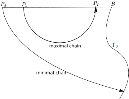
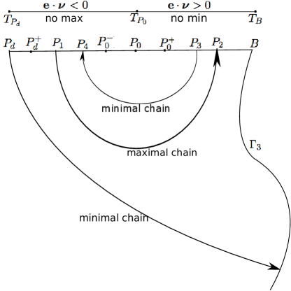
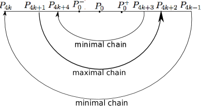
3.3   Minimal and maximal chains: Existence and properties

In this subsection, we assume that $\Omega\subset\mathbb{R}^{2}$ is open, bounded, and connected, and that $\partial\Omega$ is a continuous curve, piecewise $C^{1,\alpha}$ up to the endpoints of each smooth part and has a finite number of smooth parts. Moreover, at each corner point of $\partial\Omega$, angle $\theta$ between the arcs meeting at that point from the interior of $\Omega$ satisfies $\theta\in(0,\pi)$. Note that Theorem 2.1 requires all these conditions.

Let $\phi\in C(\overline{\Omega})\cap C^{2}(\Omega\cup\Gamma_{\text{\rm shock}}^{0})\cap C^{3}(\Omega)$ be a solution of equation (2.16) in $\Omega$ satisfying conditions (A2)–(A3) of Theorem 2.1. Let ${\mathbf{e}}\in\mathbb{R}^{2}$ be a unit vector.

Definition 3.7.

Let $E_{1},E_{2}\in\partial\Omega$. We say that points $E_{1}$ and $E_{2}$ are connected by a minimal (resp. maximal) chain with radius $r$ if there exist $r>0$, integer $k_{1}\geq 1$, and a chain of balls $\{B_{r}(C^{i})\}_{i=0}^{k_{1}}$ such that

1. $C^{0}=E_{1}$, $C^{k_{1}}=E_{2}$, and $C^{i}\in\overline{\Omega}$ for $i=0,\dots,k_{1}$;

2. $C^{i+1}\in\overline{B_{r}(C^{i})\cap\Omega}$ for $i=0,\dots,k_{1}-1$;

3. $\phi_{\mathbf{e}}(C^{i+1})={\displaystyle\min_{\overline{B_{r}(C^{i})\cap\Omega}}\phi_{\mathbf{e}}<\phi_{\mathbf{e}}(C^{i})}$ (resp. $\phi_{\mathbf{e}}(C^{i+1})={\displaystyle\max_{\overline{B_{r}(C^{i})\cap\Omega}}\phi_{\mathbf{e}}>\phi_{\mathbf{e}}(C^{i})}$) for $i=0,\dots,k_{1}-1$;

4. $\phi_{\mathbf{e}}(C^{k_{1}})={\displaystyle\min_{\overline{B_{r}(C^{k_{1}})\cap\Omega}}\phi_{\mathbf{e}}}$ (resp. $\phi_{\mathbf{e}}(C^{k_{1}})={\displaystyle\max_{\overline{B_{r}(C^{k_{1}})\cap\Omega}}\phi_{\mathbf{e}}}$).

For such a chain, we also use the following terminology: The chain starts at $E_{1}$ and ends at $E_{2}$, or the chain is from $E_{1}$ to $E_{2}$.

Remark 3.8.

This definition does not rule out the possibility that $B_{r}(C^{i})\cap\partial\Omega\neq\emptyset$, or even $C^{i}\in\partial\Omega$, for some or all $i=0,\dots,k_{1}-1$.

Remark 3.9.

Radius $r$ is a parameter in the definition of minimal or maximal chains. We do not fix $r$ at this point. In the proof of Theorems 2.1–2.3, the radii will be determined for various chains in such a way that Lemmas 3.14–3.18 below can be applied.

We now consider the minimal and maximal chains for $\phi_{\mathbf{e}}$ in $\Omega$. In the results of these subsections, all the constants depend on the parameters in the conditions listed above, i.e., the $C^{1,\alpha}$–norm of the smooth parts of $\partial\Omega$, the angles at the corner points, and $\|\phi\|_{C^{1,\alpha}(\overline{\Omega})}$, in addition to the further parameters listed in the statements.

We first show that the chains with sufficiently small radius are connected sets.

Lemma 3.10.

There exists $r^{*}>0$, depending only on the $C^{1,\alpha}$–norms of the smooth parts of $\partial\Omega$ and angles $\theta\in(0,\pi)$ in the corner points, such that, for any $E\in\overline{\Omega}$ and $r\in(0,r^{*}]$,

1. $B_{r}(E)\cap\Omega$ is connected;

2. For any $G\in\overline{B_{r}(E)\cap\Omega}$, $B_{r}(E)\cap B_{r}(G)\cap\Omega$ is nonempty.

Proof.

We only sketch the argument, since the details are standard.

We first prove (i). Denote $Q_{r}:=(-Lr,Lr)\times(-r,r)$. The conditions on $\partial\Omega$ imply that there exist $L,N>4$ such that, for any sufficiently small $r>0$, the following facts hold:

1. If $P\in\partial\Omega$ has the distance at least $Nr$ from the corner points of $\partial\Omega$, then, in some orthonormal coordinate system in $\mathbb{R}^{2}$ with the origin at $P$,

   $$\begin{split}&\Omega\cap Q_{2r}=\{(s,t)\in Q_{2r}\;:\;s>g(t)\},\\ &\partial\Omega\cap Q_{2r}=\{(s,t)\in Q_{2r}\;:\;s=g(t)\}\end{split}$$ (3.17)

   for some $g\in C^{1,\alpha}(\mathbb{R})$ with $g(0)=g^{\prime}(0)=0$;

2. If $P\in\partial\Omega$ is a corner point, then, in some orthonormal coordinate system in $\mathbb{R}^{2}$ with the origin at $P$,

   $$\begin{split}&\Omega\cap Q_{4Nr}=\{(s,t)\in Q_{4Nr}\;:\;s>\max(g_{1}(t),g_{2}(t))\},\\[2.84526pt] &\partial\Omega\cap Q_{4Nr}=\{(s,t)\in Q_{4Nr}\;:\;s=\max(g_{1}(t),g_{2}(t))\}\end{split}$$ (3.18)

   for some $g_{1}$ and $g_{2}$ satisfying

   $$\begin{split}&g_{1},g_{2}\in C^{1,\alpha}(\mathbb{R}),\;\;g_{1}(0)=g_{2}(0)=0,\;\;g_{1}^{\prime}(0)<0,\;\;g_{2}^{\prime}(0)>0,\\ &g_{1}(t)>g_{2}(t)\;\mbox{ for $t<0$},\qquad\;g_{1}(t)<g_{2}(t)\;\mbox{ for $t>0$}.\end{split}$$ (3.19)

   Note that, in order to obtain (3.18)–(3.19), we use the condition that angle $\theta$ at $P$ satisfies $\theta\in(0,\pi)$.

Let $E\in\overline{\Omega}$. Without loss of generality, we assume that ${\rm dist}(E,\partial\Omega)<r$; otherwise, (i) already holds.

The first case is that the distance from $E$ to the corner points is at least $2Nr$. Then, denoting by $P$ the nearest point on $\partial\Omega$ to $E$, it follows that $P$ satisfies the condition for Case (a) above, so that $P$ is the unique nearest point on $\partial\Omega$ to $E$, and $E=(s^{*},0)$ with $s^{*}\in[0,r)$ in the coordinate system described in (a) above. Then, denoting $f^{\pm}(t):=s^{*}\pm\sqrt{r^{2}-t^{2}}$ on $[-r,r]$, and using that $|g^{\prime}(t)|\leq Ct^{\alpha}$ and $|g(t)|\leq Ct^{1+\alpha}$ on $[-r,r]$ for $C$ depending on the $C^{1,\alpha}$–norm of the smooth parts of $\partial\Omega$, we obtain that, if $r$ is small, there exist $t^{+}\in(\frac{9}{10}r,r]$ and $t^{-}\in[-r,-\frac{9}{10}r)$ such that

$$f^{+}>g\,\,\,\mbox{on $(t^{-},t^{+})$},\qquad\,f^{+}<g\,\,\,\mbox{on $[-r,r]\setminus[t^{-},t^{+}]$},$$ (3.20)

where the last set is empty if $t^{\pm}=\pm r$, and

$$\Omega\cap B_{r}(E)=\{(s,t)\;:\;\max(f^{-}(t),g(t))<s<f^{+}(t),\;t^{-}<t<t^{+}\},$$ (3.21)

which is a connected set, by the first inequality in (3.20) and the fact that $f^{-}<f^{+}$ in $(-r,r)$.

In the other case, when the distance from $E$ to the corner points is smaller than $2Nr$, we argue similarly by using the coordinates described in Case (b) above, related to the corner point $P$ that is the nearest to $E$. The existence of such a coordinate system and the fact that ${\rm dist}(E,P)<2Nr$ also imply that the nearest corner $P$ is unique for $E$. Then, in these coordinates,

$$E=(s^{*},t^{*})\in\overline{\Omega\cap Q_{2Nr}}.$$

Let

$$\Omega^{(k)}:=\{s>g^{(k)}(t),\;\;t\in\mathbb{R}\},\,\,\,\,\Gamma^{(k)}:=\{s=g^{(k)}(t),\;\;t\in\mathbb{R}\}\qquad\mbox{ for $k=1,2$}.$$

Then, by (3.18),

$$\Omega\cap Q_{4Nr}=\Omega^{(1)}\cap\Omega^{(2)}\cap Q_{4Nr}.$$ (3.22)

If $r$ is sufficiently small, we deduce from (3.19) that there exists $\lambda\in(0,1)$ such that

$$-\lambda^{-1}\leq g_{1}^{\prime}(t)\leq-\lambda,\quad\lambda\leq g_{2}^{\prime}(t)\leq\lambda^{-1}\qquad\,\,\mbox{ for all $t\in(-4Nr,4Nr)$}.$$ (3.23)

Let $P^{(k)}=(s^{(k)},t^{(k)})$ be the nearest point to $E$ on $\Gamma^{(k)}$. Then $P^{(k)}\in\Gamma^{(k)}\cap Q_{2Nr}$.

Assume that ${{\rm dist}}(E,\Gamma^{(1)})<r$, which implies that $E\in B_{r}(P^{(1)})$. Using (3.23), $g_{1}^{\prime}(t^{(1)})<0$. Then, reducing $r$ depending on the $C^{1,\alpha}$–norm of $g_{1}$, rotating the coordinate system $(s,t)$ by angle $\arctan(|g_{1}^{\prime}(t^{(1)})|)$ clockwise, and shifting the origin into $P^{(1)}$, we conclude that, in the resulting coordinate system $(S,T)$,

$$\Omega^{(1)}\cap Q_{r}=\{(S,T)\in Q_{r}\;:\;S>G(T)\},$$

$$\Gamma^{(1)}\cap Q_{r}=\{(S,T)\in Q_{r}\;:\;S=G(T)\},$$

for some $G\in C^{1,\alpha}(\mathbb{R})$ with $G(0)=G^{\prime}(0)=0$, which is similar to (3.17). Then, arguing as in Case (a), we obtain an expression similar to (3.21) for $\Omega^{(1)}\cap B_{r}(E)$ in the $(S,T)$–coordinates. Changing back to the $(s,t)$–coordinates and possibly further reducing $r$ depending on $\lambda$, we obtain the existence of $t^{-}\in[t^{*}-r,t^{*})$ such that

$$f^{+}>g_{1}\,\,\mbox{on $(t^{-},t^{*}+r)$},\quad\,\,f^{+}<g_{1}\,\,\mbox{on $[t^{*}-r,t^{*}+r]\setminus[t^{-},t^{*}+r]$},$$ (3.24)

where the last set is empty if $t^{-}=t^{*}-r$, and

$$\Omega^{(1)}\cap B_{r}(E)=\{(s,t)\;:\;\max(f^{-}(t),g_{1}(t))<s<f^{+}(t),\;t^{-}<t<t^{*}+r\},$$ (3.25)

where $f^{\pm}(t):=s^{*}\pm\sqrt{r^{2}-(t-t^{*})^{2}}$ on $[t^{*}-r,t^{*}+r]$. Note that (3.25) also holds if ${{\rm dist}}(E,\Gamma^{(1)})\geq r$: Indeed, in this case, $\Omega^{(1)}\cap B_{r}(E)=B_{r}(E)$ and $g_{1}(t)\leq f^{-}(t)$ on $[t^{*}-r,t^{*}+r]$, so that (3.25) holds with $t^{-}=t^{*}-r$.

By a similar argument, we show the existence of $t^{+}\in(t^{*},t^{*}+r]$ such that

$$f^{+}>g_{2}\,\,\mbox{on $(t^{*}-r,t^{+})$},\quad\,\,f^{+}<g_{2}\,\,\mbox{on $[t^{*}-r,t^{*}+r]\setminus[t^{*}-r,t^{+}]$},$$ (3.26)

where the last set is empty if $t^{+}=t^{*}+r$, and

$$\Omega^{(2)}\cap B_{r}(E)=\{(s,t)\;:\;\max(f^{-}(t),g_{2}(t))<s<f^{+}(t),\;t^{*}-r<t<t^{+}\}.$$ (3.27)

From (3.22), (3.25), and (3.27), we obtain

$$\Omega\cap B_{r}(E)=\{(s,t)\;:\;\max(f^{-}(t),g_{1}(t),g_{2}(t))<s<f^{+}(t),\;t^{-}<t<t^{+}\},$$ (3.28)

which is a connected set, by the first inequalities in (3.24) and (3.26) and the fact that $f^{-}<f^{+}$ in $(t^{*}-r,t^{*}+r)$.

Now we prove assertion (ii). We can assume that $G\in B_{r}(E)\cap\partial\Omega$; otherwise, (ii) already holds. Then we again consider two cases, as above, and use expressions (3.21) and (3.28) to conclude the proof. ∎

Remark 3.11.

The condition that the interior angles $\theta$ at the corner points of $\partial\Omega$ satisfy $\theta\in(0,\pi)$ is necessary for Lemma 3.10. Indeed, let $\theta\in(\pi,2\pi)$ at some corner $Q\in\partial\Omega$. For simplicity, consider first the case when $\partial\Omega\cap B_{5R}(Q)$ consists of two straight lines intersecting at $Q$ for some $R>0$. Then it is easy to see that, for any $E\in\partial\Omega$ with $d:={\rm dist}(E,Q)\in(0,R]$, $B_{r}(E)\cap\Omega$ is not connected for all $r\in(d\sin(2\pi-\theta),\,d)$. With the assumption that $\partial\Omega$ is piecewise $C^{1,\alpha}$ up to the corner points (without assumption that $\partial\Omega\cap B_{5R}(Q)$ is piecewise-linear), the same is true for all $r\in(d_{1},d)$ for some $d_{1}\in(d\sin(2\pi-\theta),d)$ if $d$ is sufficiently small.

Lemma 3.12.

There exists $r^{*}>0$ such that any chain in Definition 3.7 with $r\in(0,r^{*})$ satisfies

1. ${\displaystyle\bigcup_{i=0}^{k_{1}}\left(B_{r}(C^{i})\cap\Omega\right)}$ is connected;

2. There exists a continuous curve ${\mathcal{S}}$ with endpoints $C^{0}$ and $C^{k_{1}}$ such that

   $${\mathcal{S}}^{0}\subset{\displaystyle\bigcup_{i=0}^{k_{1}}\left(B_{r}(C^{i})\cap\Omega\right)},\,\,\,\,\;{{\rm dist}}({\mathcal{S}}_{r},\partial\Omega)>0\qquad\;\;\mbox{for all $r>0$},$$

   where ${\mathcal{S}}_{r}={\mathcal{S}}\setminus\big{(}B_{r}(C^{0})\cup B_{r}(C^{k_{1}})\big{)}$, and ${\mathcal{S}}^{0}$ denotes the open curve that does not include the endpoints. More precisely, ${\mathcal{S}}=g([0,1])$, where $g\in C([0,1];\mathbb{R}^{2})$ and is locally Lipschitz on $(0,1)$ with $g(0)=C^{0}$, $g(1)=C^{k_{1}}$, and ${\displaystyle g(t)\in\bigcup_{i=0}^{k_{1}}\left(B_{r}(C^{i})\cap\Omega\right)}$ for all $t\in(0,1)$.

Proof.

We use $r^{*}$ in Lemma 3.10. We prove (i) by induction: We first note that $B_{r}(C^{1})\cap\Omega$ is connected by Lemma 3.10(i). Suppose that, for $m\in\{1,2,\dots,k_{1}-1\}$, ${\displaystyle A_{m}=\bigcup_{i=0}^{m}\left(B_{r}(C^{i})\cap\Omega\right)}$ is connected. We note that $A_{m}$ has a nonempty intersection with $B_{r}(C^{m+1})\cap\Omega$ by Definition 3.7(b) and Lemma 3.10(ii). Also, $B_{r}(C^{m+1})\cap\Omega$ is a connected set. Then it follows that $\displaystyle\bigcup_{i=0}^{m+1}\left(B_{r}(C^{i})\cap\Omega\right)$ is connected. This proves (i).

Assertion (ii) with reduced $r^{*}$ follows from Lemmas A.1 and A.3. ∎

Remark 3.13.

Lemma 3.12(ii) implies that ${\mathcal{S}}^{0}$ lies in the interior of $\Omega$.

Now we show the existence of minimal (resp. maximal) chains. We use $r^{*}$ from Lemma 3.12 from now on.

Lemma 3.14.

If $E_{1}\in\partial\Omega$ and is not a local minimum point (resp. maximum point) of $\phi_{\mathbf{e}}$ with respect to $\overline{\Omega}$, then, for any $r\in(0,r^{*})$, there exists a minimal (resp. maximal) chain $\{G^{i}\}_{i=0}^{k_{1}}$ for $\phi_{\mathbf{e}}$ of radius $r$ in the sense of Definition 3.7, starting at $E_{1}$, i.e., $G^{0}=E_{1}$. Moreover, $G^{k_{1}}\in\partial\Omega$ is a local minimum (resp. maximum) point of $\phi_{\mathbf{e}}$ with respect to $\overline{\Omega}$, and $\phi_{\mathbf{e}}(G^{k_{1}})<\phi_{\mathbf{e}}(E_{1})$ (resp. $\phi_{\mathbf{e}}(G^{k_{1}})>\phi_{\mathbf{e}}(E_{1})$).

Proof.

We discuss only the case of the minimal chain, since the case of the maximal chain can be considered similarly. Thus, $E_{1}$ is not a local minimum point of $\phi_{\mathbf{e}}$ with respect to $\overline{\Omega}$.

Let $G^{0}=E_{1}$. Choose $G^{i+1}$ to be the point such that the minimum of $w=\phi_{\mathbf{e}}$ in $\overline{B_{r}(G^{i})}\cap\overline{\Omega}$ is attained at $G^{i+1}$, provided that $w(G^{i+1})<w(G^{i})$; otherwise (i.e., if the minimum of $w=\phi_{\mathbf{e}}$ in $\overline{B_{r_{1}}(G^{i})}\cap\overline{\Omega}$ is attained at $G^{i}$ itself), the process ends and we set $k_{1}:=i$.

In order to show that $\{G^{i}\}_{i=0}^{k_{1}}$ is a minimal chain for $r\in(0,r^{*})$, it suffices to show that $G^{k_{1}}\in\partial\Omega$ and that $k_{1}$ is positive and finite. These can be seen as follows:

1. Since $G^{0}=E_{1}$ is not a local minimum point relative to $\overline{\Omega}$, it follows that $G^{1}\neq G^{0}$ so that $k_{1}\geq 1$ and $\phi_{\mathbf{e}}(G^{0})<\phi_{\mathbf{e}}(G^{1})$.

2. There is only a finite number of $\{G^{i}\}$. Indeed, on the contrary, since domain $\Omega$ is bounded, there exists a subsequence $\{G^{i_{m}}\}$ such that $G^{i_{m}}\rightarrow\hat{C}$ as $m\rightarrow\infty$, where $\hat{C}$ is a point lying in $\overline{\Omega}$. Thus, for any $\epsilon<r$, there is a large number $N$ such that, for any $j,\,m>N$, $\mbox{dist}\{G^{i_{j}},\,G^{i_{m}}\}<\epsilon$. On the other hand, by construction, for any $j<i-1$, $G^{i}$ cannot lie in the ball centering at $G^{j}$ with radius $r$ so that $\mbox{dist}\{G^{i},\,G^{j}\}\geq r$ for any $j<i-1$. This is a contradiction.

3. $G^{k_{1}}\in\partial\Omega$. Otherwise, $G^{k_{1}}\in\Omega$ is an interior local minimum point of $\phi_{\mathbf{e}}$, which contradicts the strong maximum principle, since $\phi_{\mathbf{e}}$ satisfies equation (3.2) that is strictly elliptic in $\Omega$, and $\phi_{\mathbf{e}}$ is not constant in $\Omega$ by the assumption that $\varphi$ is not a uniform state.

Therefore, $\{G^{i}\}_{i=0}^{k_{1}}$ is a minimal chain with $G^{k_{1}}\in\partial\Omega$. Also, from the construction, $G^{k_{1}}$ is a local minimum point of $w$ with respect to $\overline{\Omega}$ with $w(G^{k_{1}})<w(E_{1})$. ∎

Lemma 3.15.

For any $\delta>0$, there exists $r_{1}^{*}\in(0,r^{*}]$ such that the following holds: Let ${\mathcal{C}}\subset\partial\Omega$ be connected, let $E_{1}$ and $E_{2}$ be the endpoints of ${\mathcal{C}}$, and let there be a minimal chain $\{E^{i}\}_{i=0}^{k_{1}}$ of radius $r_{1}\in(0,r_{1}^{*}]$ which starts at $E_{1}$ and ends at $E_{2}$, and $H_{1}\in{\mathcal{C}}^{0}={\mathcal{C}}\setminus\{E_{1},E_{2}\}$ such that

$$\phi_{\mathbf{e}}(H_{1})\geq\phi_{\mathbf{e}}(E_{1})+\delta.$$

Then, for any $r_{2}\in(0,r_{1}]$, any maximal chain $\{H^{j}\}_{j=0}^{k_{2}}$ of radius $r_{2}$ starting from $H_{1}$ satisfies $H^{k_{2}}\in{\mathcal{C}}^{0}$, where ${\mathcal{C}}^{0}$ denotes the relative interior of curve ${\mathcal{C}}$ as before.

Proof.

Using the bound: $\|\phi\|_{1+\alpha_{1},\overline{\Omega}}\leq C$ by condition (A2) of Theorem 2.1, we can find a radius $r_{1}^{*}\in(0,r^{*}]$ small enough such that

$$\underset{B_{r_{1}^{*}}(P)\cap\Omega}{\rm osc}\,\phi_{\mathbf{e}}\leq\frac{\delta}{4}\qquad\,\,\,\mbox{for all $P\in\overline{\Omega}$}.$$

We fix this $r_{1}^{*}$ and assume that the minimal chain $\{E^{i}\}_{i=0}^{k_{1}}$ from $E_{1}$ to $E_{2}$ is of radius $r_{1}\in(0,r_{1}^{*}]$.

Recall that, from Definition 3.7 for the minimal and maximal chains, $\phi_{\mathbf{e}}(E_{1})>\phi_{\mathbf{e}}(E^{i})$ for $i=1,\dots,k_{1}$, and $\phi_{\mathbf{e}}(H_{1})<\phi_{\mathbf{e}}(H^{j})$ for $j=1,\dots,k_{2}$. Then, for each $i=0,\dots,k_{1}$, and $j=0,\dots,k_{2}$,

$$\min_{\overline{B_{r_{1}}(H^{j})\cap\Omega}}\phi_{\mathbf{e}} >\phi_{\mathbf{e}}(H^{j})-\frac{\delta}{2}\geq\phi_{\mathbf{e}}(H_{1})-\frac{\delta}{2}$$

$$\geq\phi_{\mathbf{e}}(E_{1})+\frac{\delta}{2}\geq\phi_{\mathbf{e}}(E^{i})+\frac{\delta}{2}>\max_{\overline{B_{r_{1}}(E^{i})\cap\Omega}}\phi_{\mathbf{e}}+\frac{\delta}{4},$$

where we have used that $E_{1}=E^{0}$, $H_{1}=H^{0}$, and $0<r_{1}\leq r_{1}^{*}$. Then

$$\overline{B_{r_{1}}(H^{j})\cap\Omega}\mathbin{\scalebox{1.5}{$\cap$}}\overline{B_{r_{1}}(E^{i})\cap\Omega}=\emptyset\quad\,\mbox{for each $i=0,\dots,k_{1}$, and $j=0,\dots,k_{2}$}.$$ (3.29)

From this, we have

$$B_{r_{1}}(H^{j})\cap\Omega\subset\Omega\setminus\Lambda\quad\,\,\mbox{ for each $j=1,\dots,k_{2}$},$$

where $\Lambda:=\bigcup_{i=0}^{k_{1}}\overline{B_{r_{1}}(E^{i})\cap\Omega}$.

Since $\overline{B_{r_{1}}(H^{1})\cap\Omega}$ is a connected set, then one of connected components of set $\displaystyle\overline{\Omega}\setminus\Lambda$ contains $\overline{B_{r_{1}}(H^{1})\cap\Omega}$. We denote this component by $K_{1}$. Since $\Omega$ is a connected set, then it follows from (3.29) and Lemma 3.12(i) applied to chain $\{H^{j}\}$ that

$$\bigcup_{j=0}^{k_{2}}\overline{B_{r_{2}}(H^{j})\cap\Omega}\subset K_{1}.$$

Thus, $H^{k_{2}}\in\partial K_{1}\cap\partial\Omega$. It remains to show that $\partial K_{1}\cap\partial\Omega$ lies within ${\mathcal{C}}$.

Notice that $H_{1}\in\partial K_{1}\cap{\mathcal{C}}$ so that $\partial K_{1}\cap{\mathcal{C}}\neq\emptyset$. Also, $K_{1}$ is a connected set with $K_{1}\cap\Lambda=\emptyset$. From Lemma 3.12(ii) applied to chain $\{E^{i}\}$, we obtain the existence of a continuous curve ${\mathcal{S}}\subset\Lambda$ connecting $E_{1}$ to $E_{2}$ with the properties listed in Lemma 3.12(ii). Combining these properties with Remark 3.13, we see that $K_{1}\subset\overline{\Omega}_{1}$, where $\Omega_{1}$ is the open region bounded by curves ${\mathcal{S}}$ and ${\mathcal{C}}$. Notice that $\Omega_{1}\subset\Omega$. Thus, $\partial K_{1}\cap\partial\Omega$ lies within $\partial\Omega_{1}\cap\partial\Omega={\mathcal{C}}$, which implies that $H^{k_{2}}\in{\mathcal{C}}$. Moreover, the definition of minimal and maximal chains and our assumptions in this lemma imply

$$\phi_{\mathbf{e}}(H^{k_{2}})>\phi_{\mathbf{e}}(H^{1})>\phi_{\mathbf{e}}(E_{1})>\phi_{\mathbf{e}}(E_{2}).$$

Thus, $H^{k_{2}}\in{\mathcal{C}}^{0}$. ∎

Remark 3.16.

In Lemma 3.15, we have not discussed the existence of the maximal chain $\{H^{j}\}_{j=0}^{k_{2}}$ of radius $r_{2}$ starting from $H_{1}$. If $H_{1}$ is not a local maximum point of $\phi_{\mathbf{e}}$ with respect to $\overline{\Omega}$, such an existence follows from Lemma 3.14.

We also have a version of Lemma 3.15 in which the roles of minimal and maximal chains are interchanged:

Lemma 3.17.

For any $\delta>0$, there exists $r_{1}^{*}\in(0,r^{*}]$ such that the following holds: Let ${\mathcal{C}}\subset\partial\Omega$ be connected, let $E_{1}$ and $E_{2}$ be the endpoints of ${\mathcal{C}}$, and let there exist a maximal chain $\{E^{i}\}_{i=0}^{k_{1}}$ of radius $r_{1}\in(0,r_{1}^{*}]$ which starts at $E_{1}$ and ends at $E_{2}$, and $H_{1}\in{\mathcal{C}}^{0}$ such that

$$\phi_{\mathbf{e}}(H_{1})\leq\phi_{\mathbf{e}}(E_{1})-\delta.$$

Then, for any $r_{2}\in(0,r_{1}]$, any minimal chain $\{H^{j}\}_{j=0}^{k_{2}}$ of radius $r_{2}$, starting from $H_{1}$, satisfies that $H^{k_{2}}\in{\mathcal{C}}^{0}$.

The proof follows the argument of Lemma 3.15 with the changes resulting from switching between the minimal and maximal chains and the correspondingly reversed signs in the inequalities.

Lemma 3.18.

For any $r_{1}\in(0,r^{*}]$, there exists $r_{2}^{*}=r_{2}^{*}(r_{1})\in(0,r^{*}]$ such that the following holds: Let ${\mathcal{C}}\subset\partial\Omega$ be connected, let $E_{1}$ and $E_{2}$ be the endpoints of ${\mathcal{C}}$, let there exist a minimal chain $\{E^{i}\}_{i=0}^{k_{1}}$ of radius $r_{1}\in(0,r^{*}]$ which starts at $E_{1}$ and ends at $E_{2}$, and let there exist $H_{1}\in{\mathcal{C}}^{0}$ such that

$$\phi_{\mathbf{e}}(H_{1})<\phi_{\mathbf{e}}(E_{2}).$$

Then, for any $r_{2}\in(0,r_{2}^{*}]$, any minimal chain $\{H^{j}\}_{j=0}^{k_{2}}$ of radius $r_{2}$, starting from $H_{1}$, satisfies that $H^{k_{2}}\in{\mathcal{C}}^{0}$.

Proof.

As in the proof of Lemma 3.15, we need to show (3.29). Set $\delta:=\phi_{\mathbf{e}}(E_{2})-\phi_{\mathbf{e}}(H_{1})$. Then $\delta>0$.

Using condition (A2) of Theorem 2.1, we can find a radius $r_{2}^{*}\in(0,r^{*}]$ small enough such that $\underset{B_{r_{2}^{*}}(P)\cap\Omega}{\rm osc}\,\phi_{\mathbf{e}}\leq\frac{\delta}{4}$ for all $P\in\overline{\Omega}$. We fix this $r_{2}^{*}$ and assume that the minimal chain $\{H^{j}\}_{j=0}^{k_{2}}$ starting at $H_{1}$ is of radius $r_{2}\in(0,r_{2}^{*}]$. Then, using properties (c)–(d) in Definition 3.7 for the minimal chains, we have

$$\phi_{\mathbf{e}}(E_{2})=\phi_{\mathbf{e}}(E^{k_{1}})=\min_{\overline{B_{r_{1}}(E^{k_{1}})\cap\Omega}}\phi_{\mathbf{e}}<\phi_{\mathbf{e}}(E^{k_{1}-1})=\min_{\overline{B_{r_{1}}(E^{k_{1}-1})\cap\Omega}}\phi_{\mathbf{e}}<\cdots,$$

that is,

$$\phi_{\mathbf{e}}(E_{2})\leq\min_{\overline{B_{r_{1}}(E^{i})\cap\Omega}}\phi_{\mathbf{e}}\qquad\,\,\mbox{for $i=0,\dots,k_{1}$}.$$

Then, for $i=0,\dots,k_{1}$ and $j=0,\dots,k_{2}$,

$$\max_{\overline{B_{r_{2}}(H^{j})\cap\Omega}}\phi_{\mathbf{e}}\leq\phi_{\mathbf{e}}(H^{j})+\frac{\delta}{2}\leq\phi_{\mathbf{e}}(H_{1})+\frac{\delta}{2}=\phi_{\mathbf{e}}(E_{2})-\frac{\delta}{2}\leq\min_{\overline{B_{r_{1}}(E^{i})\cap\Omega}}\phi_{\mathbf{e}}-\frac{\delta}{2}.$$

This implies (3.29). Then the rest of the proof of Lemma 3.15 applies without changes. ∎

4   Proof of Theorem 2.1

In this section, we first prove Theorem 2.1, based on the lemmas obtained in §3.

We use the $(S,T)$–coordinates from Lemma 3.2 for a unit vector $\mathbf{e}\in Con$ chosen below so that it suffices to prove that the graph of $f^{\prime\prime}_{\mathbf{e}}$ is concave:

$$f^{\prime\prime}_{\mathbf{e}}(T)\leq 0\qquad\;\mbox{for all $T\in(T_{A},T_{B})$},$$

and satisfies the strict convexity in the sense of Theorem 2.1.

In the following, we denote all the points on $\Gamma_{\text{\rm shock}}$ with respect to $T$; that is, for any point $P\in\Gamma_{\text{\rm shock}}$, there exists $T_{P}$ such that $P=(f_{\mathbf{e}}(T_{P}),T_{P})$ in the $(S,T)$–coordinates.

The proof of Theorem 2.1 consists of the following four steps, where the non-strict concavity of $f^{\prime\prime}_{\mathbf{e}}$ is shown in Steps 1–3, while the strict convexity is shown in Step 4:

1. For any fixed $\mathbf{e}\in Con$, if there exists $\hat{P}\in\Gamma_{\text{\rm shock}}^{0}$ with $f_{\mathbf{e}}^{\prime\prime}(T_{\hat{P}})>0$, we prove the existence of a point $C\in\Gamma_{\text{\rm shock}}^{0}$, depending on $\mathbf{e}$, such that $f_{\mathbf{e}}^{\prime\prime}(T_{C})\geq 0$, and $C$ is a local minimum point of $\phi_{\mathbf{e}}$ along $\Gamma_{\text{\rm shock}}$, but $C$ is not a local minimum point of $\phi_{\mathbf{e}}$ relative to $\overline{\Omega}$.

2. We fix $\mathbf{e}\in Con$ to be the vector from condition (A6). Then we prove the existence of $C_{1}\in\Gamma_{\text{\rm shock}}^{0}$ such that there exists a minimal chain with radius $r_{1}$ from $C$ to $C_{1}$.

3. Let $\mathbf{e}\in Con$ be the same as in Step 2. We show that the existence of points $C$ and $C_{1}$ described above yields a contradiction, from which we conclude that there is no $\hat{P}\in\Gamma_{\text{\rm shock}}^{0}$ with $f_{\mathbf{e}}^{\prime\prime}(T_{\hat{P}})>0$. More precisely, it will be proved by showing the following facts:

   • Let $A_{2}$ be a maximum point of $\phi_{\mathbf{e}}$ along $\Gamma_{\text{\rm shock}}$ lying between points $C$ and $C_{1}$. Then $A_{2}$ is a local maximum point of $\phi_{\mathbf{e}}$ relative to $\overline{\Omega}$, and there is no point between $C$ and $C_{1}$ on $\Gamma_{\text{\rm shock}}$ such that the tangent line at this point is parallel to the one at $A_{2}$.

   • Between $C$ and $A_{2}$, or between $C_{1}$ and $A_{2}$, there exists a local minimum point $C_{2}$ of $\phi_{\mathbf{e}}$ along $\Gamma_{\text{\rm shock}}$ such that $C_{2}\neq C$, or $C_{2}\neq C_{1}$, and $C_{2}$ is not a local minimum point of $\phi_{\mathbf{e}}$ relative to domain $\overline{\Omega}$.

   • Then, by applying the results on the minimal chains obtained in §3.3 and the facts obtained above in this step, and iterating these arguments, we can conclude our contradiction argument.

4. Fix $\mathbf{e}\in Con$. We show that, for every $P\in\Gamma_{\text{\rm shock}}^{0}$, either $f_{\mathbf{e}}^{\prime\prime}(T_{P})<0$ or there exists an even integer $k>2$ such that $f_{\mathbf{e}}^{(i)}(T_{P})=0$ for all $i=2,\dots,k-1$, and $f_{\mathbf{e}}^{(k)}(T_{P})<0$. This proves the strict convexity of the shock. We also note that $k$ is independent of the choice of $\mathbf{e}\in Con$, since, by Lemma 3.2, the above property is equivalent to the facts that $\partial_{\bm{\tau}}^{i}\phi(P)=0$ for all $i=2,\dots,k-1$, and $\partial_{\bm{\tau}}^{k}\phi(P)>0$.

Now we follow these steps to prove Theorem 2.1 in the rest of this section.

4.1   Step 1: Existence of a local minimum point $C\in\Gamma_{\text{\rm shock}}^{0}$ along $\Gamma_{\text{\rm shock}}$ in the convex part.

We choose any $\mathbf{e}\in Con$ and keep it fixed through Step 1. Assume that

There exists a point $$\hat{P}\in\Gamma_{\text{\rm shock}}^{0} f_{\mathbf{e}}^{\prime\prime}(T_{\hat{P}})>0$$ such that . (4.1)

Then, in this step, we prove that there exist points $\hat{A},\hat{B},C\in\Gamma_{\text{\rm shock}}^{0}$ such that $T_{C}\in(T_{\hat{A}},T_{\hat{B}})$ with $f_{\mathbf{e}}^{\prime\prime}(T_{C})\geq 0$, $f_{\mathbf{e}}^{\prime\prime}(T)<0$ for all $T\in(T_{\hat{A}},T_{\hat{B}})$ which are sufficiently close to $T_{\hat{A}}$ and $T_{\hat{B}}$, and

$$\phi_{\mathbf{e}}(C)=\min_{T\in[T_{\hat{A}},T_{\hat{B}}]}\phi_{\mathbf{e}}(f_{\mathbf{e}}(T),T).$$

Moreover, the minimum at $C$ is strict in the sense that

$$\phi_{\mathbf{e}}(f_{\mathbf{e}}(T),T)>\phi_{\mathbf{e}}(C)\qquad\mbox{for all $T\in(T_{\hat{A}},T_{\hat{B}})$ with $f_{\mathbf{e}}^{\prime\prime}(T)<0$}.$$

Lemma 4.1.

Let

$$I^{+}:=I^{+}(\hat{P})=(T_{A^{+}},T_{B^{+}})$$

be the maximal interval satisfying

• $I^{+}\subset(T_{A},T_{B})$,

• $T_{\hat{P}}\in I^{+}$,

• $f_{\mathbf{e}}^{\prime\prime}(T_{P})\geq 0$ for all $T_{P}\in I^{+}$,

• Maximality:  If $(T_{P_{1}},T_{P_{2}})\subset(T_{A},T_{B})$ such that $\hat{P}\in(T_{P_{1}},T_{P_{2}})$ and
  $f_{\mathbf{e}}^{\prime\prime}(T_{P})\geq 0$ for all $T_{P}\in(T_{P_{1}},T_{P_{2}})$, then $(T_{P_{1}},T_{P_{2}})\subset I^{+}$.

Note that such $I^{+}$ exists and is nonempty because $\hat{P}\in\Gamma_{\text{\rm shock}}^{0}$ and $f_{\mathbf{e}}^{\prime\prime}(T_{\hat{P}})>0$. Then

1. $T_{A}<T_{A^{+}}<T_{B^{+}}<T_{B}$,

2. $f_{\mathbf{e}}^{\prime}(T_{A^{+}})<f_{\mathbf{e}}^{\prime}(T_{\hat{P}})<f_{\mathbf{e}}^{\prime}(T_{B^{+}})$ and $f_{\mathbf{e}}^{\prime}(T_{A^{+}})\leq f_{\mathbf{e}}^{\prime}(T)\leq f_{\mathbf{e}}^{\prime}(T_{B^{+}})$ for all $T\in I^{+}$,

3. There exists an open interval $J^{+}\subset(T_{A},T_{B})$ such that $[T_{A^{+}},T_{B^{+}}]\subset J^{+}$ and

   $$f_{\mathbf{e}}^{\prime\prime}(T)<0,\,\,\,f_{\mathbf{e}}^{\prime}(T_{A^{+}})\leq f_{\mathbf{e}}^{\prime}(T)\leq f_{\mathbf{e}}^{\prime}(T_{B^{+}})\qquad\mbox{for all $T\in J^{+}\setminus\overline{I^{+}}$},$$ (4.2)

   where $J^{+}\backslash\overline{I^{+}}$ is non-empty, since $\overline{I^{+}}\subset J^{+}$ and $J^{+}$ is open.

Proof.

Assume that $T_{A^{+}}=T_{A}$. By the definition of $I^{+}$, $f_{\mathbf{e}}$ is convex on $I^{+}$. From condition (A4) of Theorem 2.1, $f_{\mathbf{e}}\in C^{2}((T_{A},T_{B}))\cap C^{1,\alpha}([T_{A},T_{B}])$. Combining these facts with $f_{\mathbf{e}}^{\prime\prime}(T_{\hat{P}})>0$, we have

$$f_{\mathbf{e}}(T_{\hat{P}})>f_{\mathbf{e}}(T_{A})+f^{\prime}_{\mathbf{e}}(T_{A})(T_{\hat{P}}-T_{A}).$$

By Lemma 3.2(i), this implies that $(A+Con)\cap\Omega\neq\emptyset$, which contradicts (A5). Then $T_{A^{+}}>T_{A}$. Similarly, $T_{B^{+}}<T_{B}$. This proves (i).

Property (ii) follows directly from the definition of $I^{+}$ and the fact that $f_{\mathbf{e}}^{\prime\prime}(T_{\hat{P}})>0$, by combining with regularity $f_{\mathbf{e}}\in C^{2}((T_{A},T_{B}))$.

It remains to show (iii). We first show that

there exists $$T_{\hat{A}_{1}}\in[T_{A},T_{A^{+}}) f_{\mathbf{e}}^{\prime\prime}<0 (T_{\hat{A}_{1}},T_{A^{+}})$$ such that on , (4.3)

where $T_{A}<T_{A^{+}}$ by (i). If (4.3) is false, then there exists a sequence $\{T^{+}_{i}\}\subset(T_{A},T_{A^{+}})$ such that $\lim_{i\to\infty}T^{+}_{i}=T_{A^{+}}$ and $f_{\mathbf{e}}^{\prime\prime}(T^{+}_{i})\geq 0$ for all $i$. Also, from the maximality part in the definition of $I^{+}$, there exists a sequence $\{T^{-}_{i}\}\subset(T_{A},T_{A^{+}})$ such that $\lim_{i\to\infty}T^{-}_{i}=T_{A^{+}}$ and $f_{\mathbf{e}}^{\prime\prime}(T^{-}_{i})<0$ for all $i$. From this, using the regularity of $f_{\mathbf{e}}$ in Lemma 3.5, it is easy to see that $f_{\mathbf{e}}^{(k)}(A^{+})=0$ for $k=2,3,\dots$, which contradicts Lemma 3.6. This proves (4.3).

Moreover, by property (ii), there exists $T_{\hat{A}}\in[T_{\hat{A}_{1}},T_{A^{+}})$ satisfying $f_{\mathbf{e}}^{\prime}(T_{\hat{A}})\leq f_{\mathbf{e}}^{\prime}(T_{B^{+}})$. Now, since $f_{\mathbf{e}}^{\prime\prime}<0$ on $(T_{\hat{A}_{1}},T_{A^{+}})$, we obtain that $f_{\mathbf{e}}^{\prime\prime}(T)<0$ and $f_{\mathbf{e}}^{\prime}(T_{A^{+}})<f_{\mathbf{e}}^{\prime}(T)\leq f_{\mathbf{e}}^{\prime}(T_{B^{+}})$ for all $T\in(T_{\hat{A}},T_{A^{+}})$.

Similarly, we show that there exists $T_{\hat{B}}\in(T_{B^{+}},T_{B}]$ such that $f_{\mathbf{e}}^{\prime\prime}(T)<0$ and $f_{\mathbf{e}}^{\prime}(T_{A^{+}})\leq f_{\mathbf{e}}^{\prime}(T)<f_{\mathbf{e}}^{\prime}(T_{B^{+}})$ for all $T\in(T_{B^{+}},T_{\hat{B}})$.

Now (iii) is proved with $J^{+}=(T_{\hat{A}},T_{\hat{B}})$. ∎

Clearly, the interval, $J^{+}$, satisfying the properties in Lemma 4.1(iii) is non-unique. From now on, we choose and fix an interval:

$$J^{+}=(T_{\hat{A}},T_{\hat{B}})$$ (4.4)

satisfying the properties stated in Lemma 4.1(iii).

Now we show the existence of a local minimum point $C\in\overline{I^{+}}$ along $\Gamma_{\text{\rm shock}}$.

Proposition 4.2.

Set

$$w:=\phi_{\mathbf{e}}.$$

Then

1. There exists $T_{C}\in\overline{I^{+}}$ such that

   $$w(C)=\min_{[T_{\hat{A}},T_{\hat{B}}]}w(f_{\mathbf{e}}(T),T){\rm;}$$

2. $C\in\Gamma_{\text{\rm shock}}^{0}$ with $f^{\prime\prime}_{\mathbf{e}}(T_{C})\geq 0$;

3. Furthermore,

   $$w(P)>w(C)\qquad\,\,\mbox{ for all $T_{P}\in(T_{\hat{A}},T_{\hat{B}})\setminus[T_{A^{+}},T_{B^{+}}]$}.$$

Proof.

Let $J^{+}$ be the open interval from (4.4), which satisfies the properties in Lemma 4.1(iii). Also, recall that $\overline{I^{+}}=[T_{A+},T_{B^{+}}]$. Then, from (i) and (iii) of Lemma 4.1, we obtain that $T_{\hat{A}}<T_{A+}<T_{B^{+}}<T_{\hat{B}}$.

Fix $T_{P}\in J^{+}\setminus\overline{I^{+}}$. Then $f^{\prime}_{\mathbf{e}}(T_{A^{+}})\leq f^{\prime}_{\mathbf{e}}(T_{P})\leq f^{\prime}_{\mathbf{e}}(T_{B^{+}})$ by Lemma 4.1(iii). Thus, there exists $T_{P_{1}}\in\overline{I^{+}}=[T_{A+},\,T_{B^{+}}]$ such that $f^{\prime}_{\mathbf{e}}(T_{P_{1}})=f^{\prime}_{\mathbf{e}}(T_{P})$. In addition, since $f_{\mathbf{e}}^{\prime\prime}\geq 0$ in $\overline{I^{+}}$ by the definition of $I^{+}$, and $f_{\mathbf{e}}^{\prime\prime}<0$ in $J^{+}\setminus[T_{A+},T_{B^{+}}]$ by Lemma 4.1(iii), then

• If $T_{P}\in[T_{B^{+}},T_{\hat{B}}]$, $f^{\prime}_{\mathbf{e}}(T)\geq f^{\prime}_{\mathbf{e}}(T_{P_{1}})$ for all $T\in[T_{P_{1}},T_{P}]$, with strict inequality $f^{\prime}_{\mathbf{e}}(T)>f^{\prime}_{\mathbf{e}}(T_{P_{1}})$ for $T\in(T_{B^{+}},T_{P})$,

• If $T_{P}\in[T_{\hat{A}},T_{A^{+}}]$, $f^{\prime}_{\mathbf{e}}(T)\leq f_{\mathbf{e}}^{\prime}(T_{P_{1}})$ for all $T\in[T_{P},T_{P_{1}}]$, with strict inequality $f^{\prime}_{\mathbf{e}}(T)<f^{\prime}_{\mathbf{e}}(T_{P_{1}})$ for $T\in(T_{P},T_{A^{+}})$.

Thus, defining the function:

$$g(T):=f_{\mathbf{e}}(T)-f_{\mathbf{e}}(T_{P_{1}})-f^{\prime}_{\mathbf{e}}(T_{P_{1}})(T-T_{P_{1}}),$$

we obtain in the two cases considered above:

• If $T_{P}\in[T_{B^{+}},T_{\hat{B}}]$, then

  $$g^{\prime}(T)\begin{cases}\geq 0\quad&\mbox{for $T\in[T_{P_{1}},T_{P}]$},\\ >0\quad&\mbox{for $T\in(T_{B^{+}},T_{P})$}.\end{cases}$$

• If $T_{P}\in[T_{\hat{A}},T_{A^{+}}]$, then

  $$g^{\prime}(T)\begin{cases}\leq 0\quad&\mbox{for $T\in[T_{P},T_{P_{1}}]$},\\ <0\quad&\mbox{for $T\in(T_{P},T_{A^{+}})$}.\end{cases}$$

Therefore, in both cases, $g(T_{P})>g(T_{P_{1}})$, which implies

$$f_{\mathbf{e}}(T_{P})>f_{\mathbf{e}}(T_{P_{1}})+f^{\prime}_{\mathbf{e}}(T_{P_{1}})(T_{P}-T_{P_{1}}).$$

Now, by Lemma 3.4,

$$w(P)>w(P_{1}).$$ (4.5)

Thus we have proved that, for any $T_{P}\in J^{+}\setminus\overline{I^{+}}$, there exists $T_{P_{1}}\in\overline{I^{+}}$ such that (4.5) holds for $P=(f_{\mathbf{e}}(T_{P}),T_{P})$ and $P_{1}=(f_{\mathbf{e}}(T_{P_{1}}),T_{P_{1}})$. This implies that there exists $T_{C}\in\overline{I^{+}}$ such that $w(f_{\mathbf{e}}(T),T)$ attains its minimum over $\overline{J^{+}}=[T_{\hat{A}},T_{\hat{B}}]$ at $T_{C}$. This proves assertion (i).

Moreover, we find from $T_{C}\in\overline{I^{+}}\subset J^{+}$ that $C\in\Gamma_{\text{\rm shock}}^{0}$. Also, from (i) and $\overline{I^{+}}\subset J^{+}=(T_{\hat{A}},T_{\hat{B}})$, $f^{\prime\prime}_{\mathbf{e}}(T_{C})\geq 0$. This proves assertion (ii).

Assertion (iii) for all $T_{P}\in(T_{\hat{A}},T_{\hat{B}})\setminus[T_{A^{+}},T_{B^{+}}]$ follows from the strict inequality in (4.5). ∎

We derive a corollary of Lemma 4.2(ii). The property, $C\in\Gamma_{\text{\rm shock}}^{0}$, guarantees the strict ellipticity of equation (2.16) at $C$, where we have used assumption (A3) of Theorem 2.1. Combining $f^{\prime\prime}_{\mathbf{e}}(T_{C})\geq 0$ with Lemma 3.2(v) implies that $\phi_{\bm{\tau}\bm{\tau}}(C)\leq 0$. Thus, from Lemma 3.1 and Lemma 3.2(iii), we obtain

Corollary 4.3.

$C$ is not a local minimum point of $\phi_{\mathbf{e}}$ with respect to $\overline{\Omega}$.

This means that, for any radius $r>0$, there is a point $C_{r}\in\overline{B_{r}(C)\cap\Omega}$ such that $w(C_{r})<w(C)$.

4.2   Step 2: Existence of $T_{C_{1}}\in(T_{A},T_{B})\setminus[T_{\hat{A}},T_{\hat{B}}]$ such that $C_{1}$ and $C$ are connected by a minimal chain with radius $r_{1}$, for vector $\mathbf{e}$ from condition (A6).

In the argument, we use the minimal and maximal chains in the sense of Definition 3.7.

Through §4.2–§4.3, we fix $\mathbf{e}\in Con$ to be the vector from condition (A6) of Theorem 2.1, and use points $\hat{A},\hat{B},C\in\Gamma_{\text{\rm shock}}^{0}$ from Step 1 (which correspond to this vector $\mathbf{e}$) and constant $r^{*}$ from Lemma 3.10. In this step, we prove the following proposition:

Proposition 4.4.

Let $\mathbf{e}\in Con$ be the vector from condition (A6) of Theorem 2.1, and let $C$ be the corresponding point obtained in Proposition 4.2. Then there exists $\hat{r}_{1}\in(0,r^{*}]$ such that, for any $r_{1}\in(0,\hat{r}_{1})$ and any minimal chain $\{C^{i}\}_{i=0}^{k_{1}}$ of radius $r_{1}$ for $w=\phi_{\mathbf{e}}$ starting from point $C$, its endpoint $C_{1}:=C^{k_{1}}$ is in $\Gamma_{\text{\rm shock}}^{0}$, i.e., $C_{1}\in\Gamma_{\text{\rm shock}}^{0}$. Moreover, $C_{1}$ is a local minimum point of $w$ relative to $\overline{\Omega}$ such that

$$w(C_{1})<w(C).$$

In order to prove Proposition 4.4, we first notice that, by Corollary 4.3 and Lemma 3.14, for any $r_{1}\in(0,r^{*})$, there exists a minimal chain $\{C^{i}\}_{i=0}^{k_{1}}$ of radius $r_{1}$ for $w=\phi_{\mathbf{e}}$ in the sense of Definition 3.7, starting at $C$, i.e., $C^{0}=C$. Moreover, $C^{k_{1}}\in\partial\Omega$ is a local minimum point of $w$ with respect to $\overline{\Omega}$, and $w(C^{k_{1}})<w(C)$.

Now, in order to complete the proof of Proposition 4.4, it suffices to prove the following lemma.

Lemma 4.5.

There exists $\hat{r}_{1}>0$ such that, if $r_{1}\in(0,\hat{r}_{1}]$, then $C^{k_{1}}\in\Gamma_{\text{\rm shock}}^{0}$.

Proof.

On the contrary, if $C^{k_{1}}\in\overline{\Gamma_{1}\cup\Gamma_{2}}$, we derive a contradiction for sufficiently small $r_{1}>0$. Now we divide the proof into five steps.

1. We first determine how small $r_{1}>0$ should be in the minimal chain $\{C^{i}\}$. Choose points $A_{1},B_{1}\in\Gamma_{\text{\rm shock}}$ such that

$$\begin{split}&T_{A_{1}}\in[T_{A},T_{C}],\;\quad\;\phi_{\mathbf{e}}(A_{1})=\max_{T\in[T_{A},\,T_{C}]}\phi_{\mathbf{e}}(f_{\mathbf{e}}(T),T),\\ &T_{B_{1}}\in[T_{C},T_{B}],\;\quad\;\phi_{\mathbf{e}}(B_{1})=\max_{T\in[T_{C},\,T_{B}]}\phi_{\mathbf{e}}(f_{\mathbf{e}}(T),T).\end{split}$$

Note that the definition of points $A_{1}$ and $B_{1}$ is independent of the choice of the minimal chain $\{C^{i}\}$ and its radius. Also, from Proposition 4.2(iii), it follows that $\phi_{\mathbf{e}}(A_{1})>\phi_{\mathbf{e}}(C)$ and $\phi_{\mathbf{e}}(B_{1})>\phi_{\mathbf{e}}(C)$. Let

$$\delta:=\min\big{\{}\phi_{\mathbf{e}}(A_{1})-\phi_{\mathbf{e}}(C),\;\phi_{\mathbf{e}}(B_{1})-\phi_{\mathbf{e}}(C)\big{\}}.$$

Then $\delta>0$. Lemma 3.15 determines $r_{1}^{*}(\delta)$, so that $r_{1}\in(0,r_{1}^{*}(\delta))$ is assumed in the minimal chain $\{C^{i}\}$.

2. We start from Case (i) of condition (A6).

Claim: Under the condition of Case (i), $A_{1}$ cannot be a local maximum point of $w=\phi_{\mathbf{e}}$ relative to $\overline{\Omega}$.

In fact, for Case (i), if $A_{1}=A$, then $A_{1}$ cannot be a local maximum point. On the other hand, if $A_{1}\neq A$, and $A_{1}$ is a local maximum point, then

$$f_{\mathbf{e}}^{\prime\prime}(T_{A_{1}})>0\qquad\mbox{in the $(S,T)$--coordinates},$$

by Lemmas 3.1–3.2. Thus, we consider the function:

$$F(T):=f_{\mathbf{e}}(T)-f_{\mathbf{e}}(T_{A_{1}})-f_{\mathbf{e}}^{\prime}(T_{A_{1}})(T-T_{A_{1}}).$$

Then $F(T_{A_{1}})=0$, $F^{\prime}(T_{A_{1}})=0$, and $F^{\prime\prime}(T_{A_{1}})>0$ so that $F(T)>0$ near $T_{A_{1}}$. Let the maximum of $F(T)$ on $[T_{A},T_{A_{1}}]$ be attained at $T_{A^{*}}$. Then $F(T_{A^{*}})>0$, which implies that $T_{A^{*}}\neq T_{A_{1}}$.

If $T_{A^{*}}\neq T_{A}$, then $F^{\prime}(T_{A^{*}})=0$, which implies that $f^{\prime}_{\mathbf{e}}(T_{A^{*}})-f^{\prime}_{\mathbf{e}}(T_{A_{1}})=0$. If $T_{A^{*}}=T_{A}$, then, using $f_{\mathbf{e}}^{\prime}(T_{A})\geq f^{\prime}_{\mathbf{e}}(T_{A_{1}})$, condition (A5), and $F^{\prime}(T_{A})\leq 0$ (since $T_{A}=T_{A^{*}}$ is a maximum point of $F(T)$ on $[T_{A},T_{A_{1}}]$), we conclude that $f_{\mathbf{e}}^{\prime}(T_{A^{*}})=f_{\mathbf{e}}^{\prime}(T_{A})=f_{\mathbf{e}}^{\prime}(T_{A_{1}})$. Thus, in both cases,

$$f^{\prime}_{\mathbf{e}}(T_{A^{*}})-f^{\prime}_{\mathbf{e}}(T_{A_{1}})=0.$$

Also, $F(T_{A^{*}})>0$ implies

$$f_{\mathbf{e}}(T_{A^{*}})>f_{\mathbf{e}}(T_{A_{1}})+f^{\prime}_{\mathbf{e}}(T_{A_{1}})(T_{A^{*}}-T_{A_{1}}).$$

Then, from Lemma 3.4, $\phi_{\mathbf{e}}(A^{*})>\phi_{\mathbf{e}}(A_{1})$, which contradicts the definition of $A_{1}$. Now the claim is proved.

3. In this step, for Case (i) of condition (A6), we obtain a contradiction to the assumption that $C^{k_{1}}\in\overline{\Gamma_{1}\cup\Gamma_{2}}$.

Since $C^{k_{1}}\in\overline{\Gamma_{1}\cup\Gamma_{2}}$ is a local minimum point of $\phi_{\mathbf{e}}$, the condition for Case (i) implies that $C^{k_{1}}\in\overline{\Gamma_{1}}\cup\{B\}$.

We first consider the case that $C^{k_{1}}\in\overline{\Gamma_{1}}\setminus\{A\}$. Since $A_{1}$ is not a local maximum point of $w=\phi_{\mathbf{e}}$, and $r_{1}\in(0,r^{*}]$, then, by Lemma 3.14, there exists a maximal chain $\{A^{j}\}_{j=0}^{k_{2}}$ of radius $r_{1}$ for $w$ in the sense of Definition 3.7, starting at $A_{1}$, i.e., $A^{0}=A_{1}$. Moreover, $A^{k_{2}}\in\partial\Omega$ is a local maximum point of $w$ with respect to $\overline{\Omega}$, and $w(A^{k_{2}})>w(A_{1})$. Furthermore, by Lemma 3.15 and the restriction for $r_{1}$ described in Step 1, it follows that one of the following three cases occurs:

1. $A^{k_{2}}$ lies on $\Gamma_{1}^{0}$ between $C^{k_{1}}$ and $A$;

2. $A^{k_{2}}=A$;

3. $A^{k_{2}}$ lies on $\Gamma_{\text{\rm shock}}^{0}$ strictly between $A$ and $C$.

Since $A^{k_{2}}$ is a local maximum point of $\phi_{\mathbf{e}}$, then it cannot lie on $\Gamma_{1}^{0}\cup\{A\}$ by the condition of Case (i). Thus, only case (c) can occur, i.e., $A^{k_{2}}$ lies on $\Gamma_{\text{\rm shock}}^{0}$ between $A$ and $C$. However, the property that $w(A^{k_{2}})>w(A_{1})$ contradicts the fact that $T_{A_{1}}$ is the maximum point of $\phi_{\mathbf{e}}(f_{\mathbf{e}}(T),T)$ on $[T_{A},T_{C}]$. Thus, the case that $C^{k_{1}}\in\overline{\Gamma_{1}}\setminus\{A\}$ is not possible.

Next, consider the case that $C^{k_{1}}=A$. Then

$$\phi_{\mathbf{e}}(C)>\phi_{\mathbf{e}}(C^{k_{1}})=\phi_{\mathbf{e}}(A),$$

so that the definition of $A_{1}$ implies that $A_{1}\neq A$. Combining with the fact that $A_{1}\neq C$ proved above, we conclude that $A_{1}$ lies on $\Gamma_{\text{\rm shock}}^{0}$ strictly between $C$ and $C^{k_{1}}=A$. Then we obtain a contradiction by following the same argument as above.

The remaining case, $C^{k_{1}}=B$, is considered similarly to the case that $C^{k_{1}}=A$. Indeed, in that argument, we have not used the condition that $A$ cannot be a local maximum point. Thus, the argument applies to the case that $C^{k_{1}}=B$, with only notational change: points $B$ and $B_{1}$ are used, instead of $A$ and $A_{1}$.

This completes the proof for Case (i) of condition (A6) of Theorem 2.1.

4. The proof for Case (ii) of condition (A6) of Theorem 2.1 is similar to Case (i). The only difference is to replace both $A$ and $A_{1}$ in the argument by $B$ and $B_{1}$.

5. Consider Case (iii) of condition (A6) of Theorem 2.1, i.e., when $\phi_{\mathbf{e}}$ cannot have a local minimum point on $\Gamma_{1}\cup\Gamma_{2}$. For the local minimum point $C^{k_{1}}\in\overline{\Gamma_{1}\cup\Gamma_{2}}$, this implies that $C^{k_{1}}\in\{A,B\}$. Then the argument is the same as for the cases: $C^{k_{1}}=A$ and $C^{k_{1}}=B$, at the end of Step 3.

Proposition 4.4 with $C_{1}=C^{k_{1}}$ follows directly from Lemma 4.5. ∎

4.3   Step 3: Existence of points $C$ and $C_{1}$ yields a contradiction

In this section, we continue to denote by $\mathbf{e}\in Con$ the vector from condition (A6) of Theorem 2.1, and use points $\hat{A},\hat{B},C\in\Gamma_{\text{\rm shock}}^{0}$ from Step 1 which correspond to this vector $\mathbf{e}$. Then, for each $r_{1}\in(0,\hat{r}_{1}]$, the corresponding point $C_{1}$ is defined in Proposition 4.4. In this step, we will arrive at a contradiction to the existence of such $C$ and $C_{1}$ if $r_{1}$ is sufficiently small. This implies that (4.1) cannot hold for $\mathbf{e}$ from condition (A6), which means that $f_{\mathbf{e}}(\cdot)$ is concave, i.e., $\Gamma_{\text{\rm shock}}$ is convex.

For $E_{1},E_{2}\in\Gamma_{\text{\rm shock}}$, denote by $\Gamma_{\text{\rm shock}}[E_{1},E_{2}]$ the part of $\Gamma_{\text{\rm shock}}$ between points $E_{1}$ and $E_{2}$, including the endpoints.

Fix $r_{1}\in(0,\hat{r}_{1}]$. This choice determines $C_{1}$. Let $A_{2}\in\Gamma_{\text{\rm shock}}[C,C_{1}]$ be such that

$$\phi_{\mathbf{e}}(A_{2})=\max_{P\in\Gamma_{\text{\rm shock}}[C,C_{1}]}\phi_{\mathbf{e}}(P).$$ (4.6)

Lemma 4.6.

There exists $\delta>0$ such that, for any $r_{1}\in(0,\hat{r}_{1}]$, the corresponding points $C$, $C_{1}$, and $A_{2}$ defined above satisfy

$$\phi_{\mathbf{e}}(A_{2})\geq\phi_{\mathbf{e}}(C)+\delta>\phi_{\mathbf{e}}(C_{1})+\delta.$$ (4.7)

Proof.

We employ Proposition 4.2 for vector $\mathbf{e}$ from condition (A6). Then, using that $\phi_{\mathbf{e}}(C)>\phi_{\mathbf{e}}(C_{1})$ by Proposition 4.4, it follows from Proposition 4.2(i) that $T_{C_{1}}\notin[T_{\hat{A}},T_{\hat{B}}]$.

Using this and (4.6), we conclude that (4.7) holds with

$$\delta=\min\big{\{}\max_{P\in\Gamma_{\text{\rm shock}}[\hat{A},C]}\phi_{\mathbf{e}}(P),\;\max_{P\in\Gamma_{\text{\rm shock}}[\hat{B},C]}\phi_{\mathbf{e}}(P)\big{\}}-\phi_{\mathbf{e}}(C),$$ (4.8)

where $\delta>0$ by Proposition 4.2(iii). Notice that the definition of points $\hat{A}$, $\hat{B}$, and $C$ is independent of $r_{1}$; see (4.4) and Proposition 4.2(i). Then the right-hand side of (4.8) is independent of $r_{1}>0$, so that $\delta>0$ is independent of $r_{1}$. ∎

The rest of the argument in this section involves only part $\Gamma_{\text{\rm shock}}[C,C_{1}]$ of the shock curve, independent of the other parts of $\partial\Omega$. Without loss of generality, we assume that $C_{1}\in\Gamma_{\text{\rm shock}}[A,C]$ so that

$$T_{C_{1}}\in[T_{A},T_{C}].$$ (4.9)

Indeed, if $C_{1}\in\Gamma_{\text{\rm shock}}[B,C]$, we re-parameterize the shock curve by

$$\Gamma_{\text{\rm shock}}=\{(\tilde{f}_{\mathbf{e}}(T),T)\;:\;-T_{B}\leq T\leq-T_{A}\},$$

where $\tilde{f}_{\mathbf{e}}(T)=f_{\mathbf{e}}(-T)$, and $T_{A}$ and $T_{B}$ are the $T$–coordinates of $A$ and $B$ with respect to the original parameterization, and then switch the notations for points $A$ and $B$. Thus, (4.9) holds in the new parametrization.

Now (4.6) has the form:

$$\phi_{\mathbf{e}}(A_{2})=\max_{T\in[T_{C_{1}},T_{C}]}\phi_{\mathbf{e}}(f_{\mathbf{e}}(T),\,T).$$ (4.10)

In particular, $T_{A_{2}}\in(T_{C_{1}},T_{C})$. See also Fig. 2.

From Lemma 4.6 and Proposition 4.4, we obtain that, for any $r_{1}\in(0,\hat{r}_{1}]$,

$$\phi_{\mathbf{e}}(A_{2})>\phi_{\mathbf{e}}(C)+\delta>\phi_{\mathbf{e}}(C_{1})+\delta.$$ (4.11)

Now we prove

Lemma 4.7.

If $r_{1}$ is sufficiently small, then

1. $A_{2}$ is a local maximum point of $\phi_{\mathbf{e}}$ with respect to $\overline{\Omega}$;

2. There is no point $Q\neq A_{2}$ between $C$ and $C_{1}$ along the shock such that the tangent line at $Q$ is parallel to the one at $A_{2}$.

Proof.

The proof consists of two steps.

1. In this step, we prove (i). We first fix $r_{1}>0$. Let $\delta$ be from Lemma 4.6, and let $r_{1}^{*}>0$ be the constant from Lemma 3.15 for this $\delta$. We fix $r_{1}=r_{1}^{*}$, and denote $C_{1}$ and $A_{2}$ as the corresponding points for this choice of $r_{1}$. Suppose that $A_{2}$ is not a local maximum point of $\phi_{\mathbf{e}}$ with respect to $\overline{\Omega}$. Using (4.11) and the existence of a minimal chain of radius $r_{1}$ from $C$ to $C_{1}$, we can apply Lemma 3.15 to obtain the existence of a maximal chain $\{A^{j}\}_{j=0}^{k_{2}}$ of radius $r_{1}$ starting from $A_{2}$ (i.e., $A_{2}=A^{0}$) such that $A^{k_{2}}$ is on $\Gamma_{\text{\rm shock}}$ between $C$ and $C_{1}$. Since $\phi_{\mathbf{e}}(A_{2})<\phi_{\mathbf{e}}(A^{k_{2}})$, we obtain a contradiction to (4.6). Thus, $A_{2}$ is a local maximum point with respect to $\overline{\Omega}$.

Figure 4.1: The graphs of function $f_{\mathbf{e}}^{\prime}(T)$

2. Now we prove (ii). We use (4.9). Assume that there is a point $Q\neq A_{2}$ between $C$ and $C_{1}$ such that the tangent line at $Q$ is parallel to the one at $A_{2}$. Since $A_{2}$ is a local maximum point of $\phi_{\mathbf{e}}$ with respect to $\overline{\Omega}$ as shown in Step 1 in this proof, we find that $f^{\prime\prime}_{\mathbf{e}}(T_{A_{2}})>0$, by Lemmas 3.1–3.2. Define

$$F(T):=f_{\mathbf{e}}(T)-f_{\mathbf{e}}(T_{A_{2}})-f_{\mathbf{e}}^{\prime}(T_{A_{2}})(T-T_{A_{2}}).$$

Then

$$F(T_{A_{2}})=F^{\prime}(T_{A_{2}})=0,\quad\;F^{\prime\prime}(T_{A_{2}})>0,$$ (4.12)

and there is a point $T_{Q}\in(T_{C_{1}},T_{A_{2}})\cup(T_{A_{2}},T_{C})$ such that $F^{\prime}(T_{Q})=0$.

If $F(T_{Q})>0$, then, by Lemma 3.4, we conclude that $\phi_{\mathbf{e}}(Q)>\phi_{\mathbf{e}}(A_{2})$, which contradicts (4.10).

If $F(T_{Q})\leq 0$, we first consider the case that $Q\in(T_{C_{1}},T_{A_{2}})$. Using ${\displaystyle\max_{T\in[T_{Q},T_{A_{2}}]}F(T)>0}$ by (4.12) so that this maximum is attained at some point $T_{Q_{1}}\in(T_{Q},T_{A_{2}})$, we obtain

$$F(T_{Q_{1}})>0,\qquad F^{\prime}(T_{Q_{1}})=0,$$

so that Lemma 3.4 can be applied to obtain that $\phi_{\mathbf{e}}(Q_{1})>\phi_{\mathbf{e}}(A_{2})$, which is a contradiction. The case that $Q\in(T_{A_{2}},T_{C})$ is considered similarly.

Therefore, point $Q$ does not exist. ∎

Figure 4.2: Proof of Step 3 of Theorem 2.1

With the facts established in Lemma 4.7, we can conclude the proof of the main assertion of Step 3 by a contradiction for sufficiently small $r_{1}>0$. The main idea of the remaining argument is illustrated in Fig. 4.2. We first notice the following facts:

Lemma 4.8.

$f_{\mathbf{e}}(T)$ satisfies the following properties:

$$f_{\mathbf{e}}^{\prime\prime}(T_{C_{1}})<0,\quad\;f_{\mathbf{e}}^{\prime\prime}(T_{A_{2}})>0,$$ (4.13)

$$f_{\mathbf{e}}^{\prime}(T)\leq f_{\mathbf{e}}^{\prime}(T_{A_{2}})\qquad\mbox{for any $T\in[T_{C_{1}},T_{A_{2}}]$},$$ (4.14)

$$f_{\mathbf{e}}^{\prime}(T)\geq f_{\mathbf{e}}^{\prime}(T_{A_{2}})\qquad\mbox{for any $T\in[T_{A_{2}},T_{C}]$}.$$ (4.15)

Proof.

Property (4.13) follows from Lemmas 3.1–3.2, since $A_{2}$ and $C_{1}$ are the local maximum and minimum points of $\phi_{\mathbf{e}}$ with respect to $\overline{\Omega}$, respectively.

To show (4.14), we note from $f_{\mathbf{e}}^{\prime\prime}(T_{A_{2}})>0$ that $f_{\mathbf{e}}^{\prime}(T)<f_{\mathbf{e}}^{\prime}(T_{A_{2}})$ in $(T_{A_{2}}-\varepsilon,\,T_{A_{2}})$ for some $\varepsilon>0$. Then, if $f_{\mathbf{e}}^{\prime}(T_{Q})>f_{\mathbf{e}}^{\prime}(T_{A_{2}})$ for some $T_{Q}\in[T_{C_{1}},T_{A_{2}})$, there exists $T_{P}\in(T_{Q},T_{A_{2}})$ with $f_{\mathbf{e}}^{\prime}(T_{P})=f_{\mathbf{e}}^{\prime}(T_{A_{2}})$, which contradicts Lemma 4.7(ii). Thus, (4.14) holds. Finally, (4.15) is proved by similar argument. ∎

Now we choose $T_{C_{2}}\in[T_{C_{1}},T_{A_{2}}]$ such that

$$\phi_{\mathbf{e}}(C_{2})=\min_{T\in[T_{C_{1}},T_{A_{2}}]}\phi_{\mathbf{e}}(f_{\mathbf{e}}(T),T).$$ (4.16)

We show that

$$\begin{cases}\phi_{\mathbf{e}}(C_{2})<\phi_{\mathbf{e}}(C_{1}),\\ \mbox{$C_{2}$ is not a local minimum point of $\phi_{\mathbf{e}}$ relative to domain $\overline{\Omega}$.}\end{cases}$$ (4.17)

To prove (4.17), we first establish the following more general property of $\Gamma_{\text{\rm shock}}$ (which will also be used in the subsequent development):

Lemma 4.9.

Assume that there exist points $E_{1}$, $E_{2}$, and $E_{3}$ on $\Gamma_{\text{\rm shock}}$ such that

1. $T_{E_{1}}<T_{E_{2}}$ and $T_{E_{3}}\in[T_{E_{1}},T_{E_{2}}]$,

2. $f_{\mathbf{e}}^{\prime\prime}(T_{E_{1}})<0$,

3. $f_{\mathbf{e}}^{\prime}(T_{E_{1}})\leq f_{\mathbf{e}}^{\prime}(T_{E_{2}})$,

4. $\phi_{\mathbf{e}}(E_{1})<\phi_{\mathbf{e}}(E_{2})$,

5. $\phi_{\mathbf{e}}(E_{3})={\displaystyle\min_{T\in[T_{E_{1}},T_{E_{2}}]}\phi_{\mathbf{e}}(f_{\mathbf{e}}(T),T)}$.

Then $\phi_{\mathbf{e}}(E_{3})<\phi_{\mathbf{e}}(E_{1})$, and $E_{3}$ is not a local minimum point of $\phi_{\mathbf{e}}$ relative to domain $\overline{\Omega}$.

Proof.

We divide the proof into two steps.

1. We first show that $\phi_{\mathbf{e}}(E_{3})<\phi_{\mathbf{e}}(E_{1})$. By condition (v), this is equivalent to the inequality:

$$\phi_{\mathbf{e}}(E_{1})>\min_{T\in[T_{E_{1}},T_{E_{2}}]}\phi_{\mathbf{e}}(f_{\mathbf{e}}(T),T).$$

Thus, it suffices to show that it is impossible that

$$\phi_{\mathbf{e}}(E_{1})=\min_{T\in[T_{E_{1}},T_{E_{2}}]}\phi_{\mathbf{e}}(f_{\mathbf{e}}(T),T).$$ (4.18)

Assume that (4.18) holds. Consider the function:

$$F(T)=f_{\mathbf{e}}(T)-f_{\mathbf{e}}(T_{E_{1}})-f_{\mathbf{e}}^{\prime}(T_{E_{1}})(T-T_{E_{1}}).$$

Then $F(T_{E_{1}})=F^{\prime}(T_{E_{1}})=0$, and $F^{\prime\prime}(T_{E_{1}})=f_{\mathbf{e}}^{\prime\prime}(T_{E_{1}})<0$ by condition (ii). This implies that $F(T)<0$ in $(T_{E_{1}},T_{E_{1}}+\delta)$ for some small $\delta>0$. Denoting by $T_{Q}$ a minimum point of $F(T)$ in $[T_{E_{1}},T_{E_{2}}]$, then $F(T_{Q})<0$. This implies that $Q\neq E_{1}$. Now we consider two cases:

If $Q\neq E_{2}$, then $F^{\prime}(T_{Q})=0$, i.e., $f_{\mathbf{e}}^{\prime}(T_{Q})=f_{\mathbf{e}}^{\prime}(T_{E_{1}})$. With this, $F(T_{Q})<0$ can be rewritten as

$$f_{\mathbf{e}}(T_{E_{1}})>f_{\mathbf{e}}(T_{Q})+f_{\mathbf{e}}^{\prime}(T_{Q})(T_{E_{1}}-T_{Q}).$$

Then, by Lemma 3.4(ii), we obtain that $\phi_{\mathbf{e}}(E_{1})>\phi_{\mathbf{e}}(Q)$, which contradicts (4.18).

If $Q=E_{2}$, then $F^{\prime}(T_{E_{2}})\leq 0$. Notice that $F^{\prime}(T_{E_{2}})=f^{\prime}_{\mathbf{e}}(T_{E_{2}})-f^{\prime}_{\mathbf{e}}(T_{E_{1}})\geq 0$ by condition (iii). Thus, $F^{\prime}(T_{E_{2}})=0$, which means that $f^{\prime}_{\mathbf{e}}(T_{E_{2}})=f^{\prime}_{\mathbf{e}}(T_{E_{1}})$. Then, using $F(T_{E_{2}})=F(T_{Q})<0$ and arguing similar to the previous case, we employ Lemma 3.4(ii) to obtain that $\phi_{\mathbf{e}}(E_{1})>\phi_{\mathbf{e}}(E_{2})$, a contradiction to (4.18).

Therefore, we have proved that (4.18) is false. This implies that $\phi_{\mathbf{e}}(E_{3})<\phi_{\mathbf{e}}(E_{1})$, as we have shown above.

2. We now show that $E_{3}$ cannot be a local minimum point of $\phi_{\mathbf{e}}$ relative to domain $\overline{\Omega}$. We have shown in Step 1 that $E_{3}\neq E_{1}$. Also, $E_{3}\neq E_{2}$ by conditions (iv)–(v). Thus, $T_{E_{3}}\in(T_{E_{1}},T_{E_{2}})$, i.e., $E_{3}\in\Gamma_{\text{\rm shock}}^{0}$. If $E_{3}$ is a local minimum point of $\phi_{\mathbf{e}}$ relative to $\overline{\Omega}$, we obtain by Lemmas 3.1 and 3.2(v) that $f^{\prime\prime}_{\mathbf{e}}(T_{E_{3}})<0$. Let

$$G(T):=f_{\mathbf{e}}(T)-f_{\mathbf{e}}(T_{E_{3}})-f^{\prime}_{\mathbf{e}}(T_{E_{3}})(T-T_{E_{3}}).$$

Then $G(T_{E_{3}})=G^{\prime}(T_{E_{3}})=0$ and $G^{\prime\prime}(T_{E_{3}})=f_{\mathbf{e}}^{\prime\prime}(T_{E_{3}})<0$. This implies that $G(T)<0$ in $(T_{E_{3}},T_{E_{3}}+\delta)$ for some $\delta>0$. Assume that $T_{Q_{1}}$ is a minimum point of $G(T)$ in $[T_{E_{3}},T_{E_{2}}]$. Then, repeating the argument in Step 1 (with $E_{3}$, $G$, and $T_{Q_{1}}$ instead of $E_{1}$, $F$, and $T_{Q}$, respectively), we obtain that $\phi_{\mathbf{e}}(E_{3})>\phi_{\mathbf{e}}(Q_{1})$, which contradicts condition (v). ∎

Lemma 4.9 also holds if $T_{E_{1}}>T_{E_{2}}$, with only change in the condition that $f_{\mathbf{e}}^{\prime}(T_{E_{1}})\leq f_{\mathbf{e}}^{\prime}(T_{E_{2}})$ that is now replaced by $f_{\mathbf{e}}^{\prime}(T_{E_{1}})\geq f_{\mathbf{e}}^{\prime}(T_{E_{2}})$. More precisely, we have

Corollary 4.10.

Assume that there exist points $E_{1}$, $E_{2}$, and $E_{3}$ on $\Gamma_{\text{\rm shock}}$ such that

1. $T_{E_{1}}>T_{E_{2}}$ and $T_{E_{3}}\in[T_{E_{2}},T_{E_{1}}]$,

2. $f_{\mathbf{e}}^{\prime\prime}(T_{E_{1}})<0$,

3. $f_{\mathbf{e}}^{\prime}(T_{E_{1}})\geq f_{\mathbf{e}}^{\prime}(T_{E_{2}})$,

4. $\phi_{\mathbf{e}}(E_{1})<\phi_{\mathbf{e}}(E_{2})$,

5. $\phi_{\mathbf{e}}(E_{3})=\min_{T\in[T_{E_{2}},T_{E_{1}}]}\phi_{\mathbf{e}}(f_{\mathbf{e}}(T),T)$.

Then $\phi_{\mathbf{e}}(E_{3})<\phi_{\mathbf{e}}(E_{1})$, and $E_{3}$ is not a local minimum point of $\phi_{\mathbf{e}}$ relative to domain $\overline{\Omega}$.

Proof.

We prove this by directly repeating the argument in the proof of Lemma 4.9 with some obvious changes. Alternatively, by re-parameterizing the shock curve by

$$\Gamma_{\text{\rm shock}}=\{(\tilde{f}_{\mathbf{e}}(T),T)\;:\>-T_{B}\leq T\leq-T_{A}\}$$

so that $\tilde{f}_{\mathbf{e}}(T)=f_{\mathbf{e}}(-T)$, and $T_{A}$ and $T_{B}$ are the $T$–coordinates of $A$ and $B$ with respect to the original parameterization, then we are under the conditions of Lemma 4.9 in the new parameterization. ∎

Proof of (4.17).

Using (4.9)–(4.11), (4.13)–(4.14), and (4.16), we can apply Lemma 4.9 with $E_{1}=C_{1}$, $E_{2}=A_{2}$, and $E_{3}=C_{2}$ to obtain (4.17). ∎

Let $r_{1}$ be the constant from Lemma 4.7, and $r_{2}\in(0,r_{1})$. Since $C_{2}$ is not a local minimum point by (4.17), we use Lemma 3.14 to obtain the existence of a minimal chain $\{C_{2}^{j}\}_{j=0}^{k_{2}}$ with radius $r_{2}$; see Fig. 4.2. Next, we restrict $r_{2}$ to be smaller than $r_{2}^{*}$ from Lemma 3.18 defined by $r_{1}$ fixed above. Then, recalling that there is a minimal chain of radius $r_{1}$ which starts at $C$ and ends at $C_{1}$, and noting that $\phi_{\mathbf{e}}(C_{2})<\phi_{\mathbf{e}}(C_{1})$ by (4.16)–(4.17), we obtain that $C_{2}^{k_{2}}$ lies on $\Gamma_{\text{\rm shock}}$ between $C$ and $C_{1}$. Now, using (4.16) and noting that $\phi_{\mathbf{e}}(C_{2}^{k_{2}})<\phi_{\mathbf{e}}(C_{2}^{0})=\phi_{\mathbf{e}}(C_{2})$, we conclude that $C_{2}^{k_{2}}$ lies on the part $[T_{A_{2}},T_{C}]$ of $\Gamma_{\text{\rm shock}}$; see Fig. 4.2. Denote $C_{3}:=C_{2}^{k_{2}}$ and notice that $C_{3}$ is a local minimum point of $\phi_{\mathbf{e}}$ relative to $\overline{\Omega}$.

From this construction, point $A_{2}$ (defined by equation (4.6) so that (4.10) holds) satisfies $T_{A_{2}}\in(T_{C_{2}},T_{C_{3}})\subset(T_{C_{1}},T_{C})$. Then

$$\phi_{\mathbf{e}}(A_{2})=\max_{T\in[T_{C_{1}},T_{C}]}\phi_{\mathbf{e}}(f_{\mathbf{e}}(T),T)=\max_{T\in[T_{C_{2}},T_{C_{3}}]}\phi_{\mathbf{e}}(f_{\mathbf{e}}(T),T).$$

Also, from (4.11), (4.16), and the definition of $C_{3}$ as the endpoint of the minimal chain from $C_{2}$, we have

$$\phi_{\mathbf{e}}(A_{2})>\phi_{\mathbf{e}}(C_{2})>\phi_{\mathbf{e}}(C_{3}),\quad f^{\prime\prime}_{\mathbf{e}}(C_{3})\leq 0,$$

where the last property holds by Lemmas 3.1–3.2, since $C_{3}$ is a local minimum point of $\phi_{\mathbf{e}}$ with respect to $\overline{\Omega}$. Moreover, from (4.15),

$$f_{\mathbf{e}}^{\prime}(T_{C_{3}})\geq f_{\mathbf{e}}^{\prime}(T_{A_{2}}).$$

Choosing $T_{C_{4}}\in[T_{A_{2}},T_{C_{3}}]$ such that

$$\phi_{\mathbf{e}}(C_{4})=\min_{T\in[T_{A_{2}},T_{C_{3}}]}\phi_{\mathbf{e}}(f_{\mathbf{e}}(T),T),$$ (4.19)

we can apply Corollary 4.10 with $E_{1}=C_{3}$, $E_{2}=A_{2}$, and $E_{3}=C_{4}$ to show that $\phi_{\mathbf{e}}(C_{4})<\phi_{\mathbf{e}}(C_{3})$ and $C_{4}$ cannot be a local minimum point.

Then we repeat the same argument as those for the minimal chain starting from $C_{2}$. Specifically, for any $r_{3}\in(0,r_{2}]$, we use Lemma 3.14 to obtain the existence of a minimal chain $\{C_{4}^{m}\}_{m=0}^{k_{3}}$ with radius $r_{3}$ starting from $C_{4}$, i.e., $C_{4}^{0}=C_{4}$; see Fig. 4.2. Next, we restrict $r_{3}$ to be smaller than $r_{2}^{*}(r_{2})$ from Lemma 3.18, i.e., $r_{2}$ fixed above is used as $r_{1}$ in Lemma 3.18 to determine $r_{2}^{*}(r_{2})$. Then, recalling that there is a minimal chain of radius $r_{2}$ which starts at $C_{2}$ and ends at $C_{3}$, and noting that $\phi_{\mathbf{e}}(C_{4})<\phi_{\mathbf{e}}(C_{3})$ as we have shown above, we obtain by Lemma 3.18 that

$$C_{4}^{k_{3}}\,\, \Gamma_{\text{\rm shock}} C_{2} C_{3}$$ lies on between and . (4.20)

However, combining the properties shown above, we have

$$\phi_{\mathbf{e}}(C_{4}) =\min_{T\in[T_{A_{2}},T_{C_{3}}]}\phi_{\mathbf{e}}(f_{\mathbf{e}}(T),T)<\phi_{\mathbf{e}}(C_{3})$$

$$<\phi_{\mathbf{e}}(C_{2})=\min_{T\in[T_{C_{1}},T_{A_{2}}]}\phi_{\mathbf{e}}(f_{\mathbf{e}}(T),T),$$

so that

$$\phi_{\mathbf{e}}(C_{4})=\min_{T\in[T_{C_{1}},T_{C_{3}}]}\phi_{\mathbf{e}}(f_{\mathbf{e}}(T),T).$$

Then the property that $\phi_{\mathbf{e}}(C_{4}^{k_{3}})<\phi_{\mathbf{e}}(C_{4})$ implies that $C^{k_{3}}_{4}$ cannot lie on $[T_{C_{2}},T_{C_{3}}]\subset[T_{C_{1}},T_{C_{3}}]$. This contradicts (4.20).

This contradiction shows that (4.1) cannot hold if $\mathbf{e}$ is the vector from condition (A6) of Theorem 2.1. Therefore, in the $(S,T)$–coordinates from Lemma 3.2 for this vector $\mathbf{e}$, we conclude that

$$f_{\mathbf{e}}^{\prime\prime}(T)\leq 0\qquad\mbox{for all $T\in(T_{A},T_{B})$}.$$

We thus completed the proof of the following fact:

Proposition 4.11.

Suppose that conditions (A1)–(A6) of Theorem 2.1 hold. Then the free boundary $\Gamma_{\text{\rm shock}}$ is a convex graph as described in Theorem 2.1.

4.4   Step 4: Strict convexity of $\Gamma_{\text{\rm shock}}$

In this step, we show the strict convexity in the sense that, for any fixed $\mathbf{e}\in Con$, using the coordinates and function $f_{\mathbf{e}}$ from Lemma 3.2(i), for every $P\in\Gamma_{\text{\rm shock}}^{0}$, either $f_{\mathbf{e}}^{\prime\prime}(T_{P})<0$ or there exists an even integer $k>2$ such that $f_{\mathbf{e}}^{(i)}(T_{P})=0$ for all $i=2,\dots,k-1$, and $f_{\mathbf{e}}^{(k)}(T_{P})<0$.

Note that $f_{\mathbf{e}}^{\prime\prime}\leq 0$ on $(T_{A},T_{B})$ by Proposition 4.11.

Let $T_{P}\in(T_{A},T_{B})$ be such that $f_{\mathbf{e}}^{\prime\prime}(T_{P})=0$. By Lemma 3.6, there exists an integer $k$ such that

$$f_{\mathbf{e}}^{(i)}(T_{P})=0\,\,\,\,\mbox{for $i=2,\,.\,.\,.\,,\,k-1$},\qquad\,f^{(k)}_{\mathbf{e}}(T_{P})\,\,\,\mbox{is nonzero}.$$

The convexity of the shock in Proposition 4.11 implies that $k$ must be even and $f^{(k)}_{\mathbf{e}}(T_{P})<0$. This shows (2.19) in the coordinate system with basis $\{\mathbf{e},\mathbf{e}^{\perp}\}$. Moreover, using Remark 2.6, we have

Proposition 4.12.

Suppose that conditions (A1)–(A6) of Theorem 2.1 hold. Then the free boundary $\Gamma_{\text{\rm shock}}$ is strictly convex in the sense that (2.19) holds at every $T\in(T_{A},T_{B})$ with $f^{\prime\prime}(T)=0$. Moreover, (2.20) holds at every point of $\Gamma_{\text{\rm shock}}^{0}$, at which $\phi_{\bm{\tau}\bm{\tau}}=0$.

Furthermore, we note the following fact:

Lemma 4.13.

Suppose that conditions (A1)–(A6) of Theorem 2.1 hold. Then, for any $\varepsilon>0$, there is no more than a finite set of points $P=(f(T),T)\in\Gamma_{\text{\rm shock}}$ with $T\in[T_{A}+\varepsilon,T_{B}-\varepsilon]$ such that $f^{\prime\prime}(T)=0$ (or equivalently, $\phi_{\bm{\tau}\bm{\tau}}(P)=0$).

Proof.

Suppose that $T_{i}\in[T_{A}+\varepsilon,T_{B}-\varepsilon]$ for $i=1,2,\dots$, are such that $f^{\prime\prime}(T_{i})=0$. Then a subsequence of $T_{i}$ converges to $T^{*}\in[T_{A}+\varepsilon,T_{B}-\varepsilon]$, and $f^{(n)}(T^{*})=0$ for each $n=2,3,\dots$, and $P^{*}=(f(T^{*}),T^{*})\in\Gamma_{\text{\rm shock}}^{0}$. It follows that $\partial^{n}_{\bm{\tau}}\phi(P^{*})=0$ for each $n=2,3,\dots$. This contradicts (2.20). ∎

By Propositions 4.11–4.12 and Lemma 4.13, the proof of Theorem 2.1 is completed.

5   Proof of Theorem 2.3: Uniform Convexity of Transonic Shocks

In this section, we show the uniform convexity of $\Gamma_{\text{\rm shock}}^{0}$ in the sense that $f^{\prime\prime}(T_{P})<0$ for every $P\in\Gamma_{\text{\rm shock}}^{0}$ for $f(\cdot)$ in (2.18), or equivalently, $f^{\prime\prime}_{\mathbf{e}}(T)<0$ on $(T_{A},T_{B})$ for any $\mathbf{e}\in Con$.

The outline of the proof is the following: By Theorem 2.1 and Remark 2.6, $\phi_{\bm{\tau}\bm{\tau}}\geq 0$ on $\Gamma_{\text{\rm shock}}^{0}$. Thus, we need to show that $\phi_{\bm{\tau}\bm{\tau}}>0$ on $\Gamma_{\text{\rm shock}}^{0}$. Assume that $\phi_{\bm{\tau}\bm{\tau}}=0$ at $P_{\rm d}\in\Gamma_{\text{\rm shock}}^{0}$. Then we obtain a contradiction by proving that there exists a unit vector $\mathbf{e}\in\mathbb{R}^{2}$ such that $P_{\rm d}$ is a local minimum point of $\phi_{\mathbf{e}}$ along $\Gamma^{0}_{\rm shock}$, but $P_{\rm d}$ is not a local minimum point of $\phi_{\mathbf{e}}$ relative to $\overline{\Omega}$. Then we can construct a minimal chain for $\phi_{\mathbf{e}}$ connecting $P_{\rm d}$ to $C^{k_{1}}\in\partial\Omega$. We show that

• $C^{k_{1}}\notin\Gamma_{0}\cup\Gamma_{3}$,

• $C^{k_{1}}\notin\Gamma_{1}\cup\Gamma_{2}$,

• $C^{k_{1}}\notin\Gamma_{\text{\rm shock}}$.

This implies that $\phi_{\bm{\tau}\bm{\tau}}>0$ on $\Gamma_{\text{\rm shock}}^{0}$ so that $f^{\prime\prime}(T)<0$ on $(T_{A},T_{B})$; see Remark 2.6.

Now we follow the procedure outlined above to prove Theorem 2.3. In the proof, we use the $(S,T)$–coordinates in (2.18). Then we have

$$\begin{split}&\Gamma_{\text{\rm shock}}=\{S=f(T)\,:\,T_{A}<T<T_{B}\},\quad\,\Omega\subset\{S<f(T):\,T\in\mathbb{R}\},\\ &\bm{\tau}=\frac{(f^{\prime}(T),1)}{\sqrt{(f^{\prime}(T))^{2}+1}},\,\,\,\bm{\nu}=\frac{(-1,f^{\prime}(T))}{\sqrt{(f^{\prime}(T))^{2}+1}},\,\,\,f^{\prime\prime}(T)\leq 0\qquad\mbox{on $(T_{A},T_{B})$},\end{split}$$ (5.1)

where we have used the convexity of $\Gamma_{\text{\rm shock}}$ proved in Theorem 2.1. Note that the orientation of the tangent vector $\bm{\tau}(P)$ at $P\in\Gamma_{\text{\rm shock}}$ has been chosen to be towards endpoint $B$.

First, from the convexity and Lemma 3.1, we have

Lemma 5.1.

Let $\phi$ be a solution as in Theorem 2.1. For any unit vector $\mathbf{e}\in\mathbb{R}^{2}$, if $\mathbf{e}\cdot\bm{\nu}<0$ (resp. $\mathbf{e}\cdot\bm{\nu}>0$) at $P\in\Gamma_{\text{\rm shock}}^{0}$, then $\phi_{\mathbf{e}}$ cannot attain its local maximum (resp. minimum) with respect to $\overline{\Omega}$ at this point.

We now prove the uniform convexity by a contradiction argument. From Theorem 2.1 and Remark 2.6, we know that (2.20) holds so that, if $f^{\prime\prime}(T_{P_{\rm d}})=0$ at some interior point $P_{\rm d}$ of $\Gamma_{\text{\rm shock}}$, then

$$\begin{split}&\phi_{\bm{\tau}\bm{\tau}}(P_{\rm d})=0,\\ &\phi_{\bm{\tau}\bm{\tau}}(P)>0\quad\mbox{ for all $P\in\Gamma_{\text{\rm shock}}\cap{\mathcal{N}}_{\varepsilon}(P_{\rm d})$ with $P\neq P_{\rm d}$},\end{split}$$ (5.2)

for some $\varepsilon>0$. First we choose a unit vector $\mathbf{e}\in\mathbb{R}^{2}$ via the following lemma.

Lemma 5.2.

There exists a unit vector $\mathbf{e}\in\mathbb{R}^{2}$ such that, for any local minimum point $P_{\rm d}$ of $\phi_{\mathbf{e}}$ along $\Gamma^{0}_{\rm shock}$, $\mathbf{e}\cdot\bm{\nu}(P_{\rm d})<0$. In addition, $P_{\rm d}$ is a strict local minimum point along $\Gamma^{0}_{\rm shock}$ in the following sense: For the unit tangent vector $\bm{\tau}=\bm{\tau}(P)$ to $\Gamma_{\text{\rm shock}}$ at $P$ defined by (5.1), $\phi_{\mathbf{e}\bm{\tau}}$ is strictly positive on $\Gamma_{\text{\rm shock}}$ near $P_{\rm d}$ in the direction of $\bm{\tau}$, and $\phi_{\mathbf{e}\bm{\tau}}$ is strictly negative on $\Gamma_{\text{\rm shock}}$ near $P_{\rm d}$ in the direction opposite to $\bm{\tau}$. More precisely, in the coordinates from (5.1), there exists $\varepsilon>0$ such that $T_{A}<T_{P_{\rm d}}-\varepsilon<T_{P_{\rm d}}+\varepsilon<T_{B}$ and

$$\begin{split}&\phi_{\mathbf{e}\bm{\tau}}(f(T),T)<0\quad\,\,\,\mbox{on $(T_{P_{\rm d}}-\varepsilon,\,T_{P_{\rm d}})$},\\ &\phi_{\mathbf{e}\bm{\tau}}(f(T),T)>0\quad\,\,\,\mbox{on $(T_{P_{\rm d}},\,T_{P_{\rm d}}+\varepsilon)$}.\end{split}$$ (5.3)

Proof.

Recall that $\phi_{\bm{\tau}\bm{\tau}}(P_{\rm d})=0$. Now we first use (3.15) at $P_{\rm d}$ with $h_{\bm{\nu}}\neq 0$ by (3.6), and then use the strictly elliptic equation (3.1) at $P_{\rm d}$ in the $(S,T)$–coordinates with basis $\{\bm{\nu}(P_{\rm d}),\bm{\tau}(P_{\rm d})\}$ to obtain

$$\phi_{\bm{\nu}\bm{\nu}}(P_{\rm d})=\phi_{\bm{\nu}\bm{\tau}}(P_{\rm d})=\phi_{\bm{\tau}\bm{\tau}}(P_{\rm d})=0.$$ (5.4)

For any unit vector $\mathbf{e}\in\mathbb{R}^{2}$, define a function $g(\cdot)\equiv g(\mathbf{e})(\cdot)$ on $\Gamma_{\text{\rm shock}}^{0}$ by

$$g(\mathbf{e})(\bm{\xi}):=\big{(}\rho(c^{2}-\varphi_{\bm{\nu}}^{2})\varphi_{\bm{\nu}}(\mathbf{e}\cdot\bm{\tau})+(\rho\varphi^{2}_{\bm{\nu}}+\rho_{0}c^{2})\varphi_{\bm{\tau}}(\mathbf{e}\cdot\bm{\nu})\big{)}(\bm{\xi}).$$ (5.5)

Then, at any point of $\Gamma_{\text{\rm shock}}^{0}$, we see from (3.15) with (3.5) that, for any unit vector $\mathbf{e}\in\mathbb{R}^{2}$,

$$\phi_{\mathbf{e}\bm{\tau}}=\phi_{\bm{\tau}\bm{\tau}}(\mathbf{e}\cdot\bm{\tau})+\phi_{\bm{\tau}\bm{\nu}}(\mathbf{e}\cdot\bm{\nu})=\frac{\phi_{\bm{\tau}\bm{\tau}}g(\mathbf{e})}{\rho(c^{2}-\varphi^{2}_{\bm{\nu}})\varphi_{\bm{\nu}}}.$$ (5.6)

Notice that, from the expression of $g(\mathbf{e})(\cdot)$ and assumption (A3) of Theorem 2.1,

$$g(\bm{\tau})>0,\quad g(-\bm{\tau})<0\,\,\qquad\text{ on $\Gamma_{\text{\rm shock}}^{0}$}.$$ (5.7)

Then we can choose a unit vector $\mathbf{e}$ such that $\mathbf{e}\cdot\bm{\nu}<0$ and $g(\mathbf{e})=0$ at $P_{\rm d}$. We fix this vector $\mathbf{e}$ for the rest of this proof. From (5.4), we have

$$\varphi_{\bm{\tau}\bm{\tau}}=\varphi_{\bm{\nu}\bm{\nu}}=-1,\quad\varphi_{\bm{\nu}\bm{\tau}}=0\qquad\,\,\mbox{at $P_{\rm d}$}.$$ (5.8)

Below we use the $(S,T)$–coordinates from (5.1). From (2.17) and (5.1), we use condition (A1) in Theorem 2.1 to obtain that $\phi_{S}>0$ on $\Gamma_{\text{\rm shock}}$ so that

$$\bm{\tau}=\frac{(-\phi_{T},\phi_{S})}{|D\phi|},\quad\bm{\nu}=-\frac{D\phi}{|D\phi|}.$$

Then we can use these expressions to define $\bm{\tau}$ and $\bm{\nu}$ in $\Omega$ near $\Gamma_{\text{\rm shock}}$, which allows to extend function $g(\mathbf{e})(\cdot)$ defined by expression (5.5) into this region. Since $\phi\in C^{2}(\Omega\cup\Gamma_{\text{\rm shock}}^{0})$, the extended $\bm{\tau}$, $\bm{\nu}$, and $g(\mathbf{e})(\cdot)$ are $C^{1}$ up to $\Gamma_{\text{\rm shock}}^{0}$. Then, from (5.4), $D_{(S,T)}\bm{\tau}=0$ and $D_{(S,T)}\bm{\nu}=0$ at point $P_{\rm d}$. Moreover, differentiating (2.4) and (2.7), and using (5.4) yield that $D_{(S,T)}\rho=0$ and $D_{(S,T)}c^{2}=0$ at point $P_{\rm d}$. Therefore, differentiating (5.5), using (5.8), and writing $g(\cdot)$ for $g(\mathbf{e})(\cdot)$, we have

$$g_{\bm{\tau}}(P_{\rm d})=-(\mathbf{e}\cdot\bm{\nu})(\rho\varphi_{\bm{\nu}}^{2}+\rho_{0}c^{2})\Big{|}_{P_{\rm d}}>0.$$

Then, by (5.1),

$$\frac{\mathrm{d}g(f(T),T)}{\mathrm{d}T}\Big{|}_{T=T_{P_{\rm d}}}=\sqrt{(f^{\prime}(T_{P_{\rm d}}))^{2}+1}\,g_{\bm{\tau}}(P_{\rm d})>0.$$

Thus, $g(f(T),T)<0$ on $(T_{P_{\rm d}}-\varepsilon,\,T_{P_{\rm d}})$ and $g(f(T),T)>0$ on $(T_{P_{\rm d}},\,T_{P_{\rm d}}+\varepsilon)$ for some $\varepsilon>0$. By (5.2) and (5.6), the same is true for $\phi_{\mathbf{e}\bm{\tau}}$.

Then $P_{\rm d}$ is a local minimum point of $\phi_{\mathbf{e}}$ along $\Gamma_{\rm shock}$, and $\phi_{\mathbf{e}\bm{\tau}}$ has the properties asserted. ∎

Remark 5.3.

The unit vector $\mathbf{e}$ is not necessarily in the cone introduced in condition (A5) of Theorem 2.1.

Lemma 5.4.

$P_{\rm d}$ is not a local minimum point of $\phi_{\mathbf{e}}$ with respect to $\overline{\Omega}$.

Proof.

If $P_{\rm d}$ is a local minimum point, it follows from Lemma 3.1 and $\mathbf{e}\cdot\bm{\nu}(P_{\rm d})<0$ that $\phi_{\bm{\tau}\bm{\tau}}(P_{\rm d})>0$, which contradicts to the fact that $\phi_{\bm{\tau}\bm{\tau}}(P_{\rm d})=0$. ∎

Now we consider a minimal chain starting at $P_{\rm d}$. In the following argument, we use the $(S,T)$–coordinates in (5.1).

To choose the radius for this chain, we note the following:

Lemma 5.5.

There exist points $P_{\rm d}^{\pm}\in\Gamma_{\text{\rm shock}}^{0}$ such that

1. $P_{\rm d}$ lies on $\Gamma_{\text{\rm shock}}$ strictly between $P_{\rm d}^{+}$ and $P_{\rm d}^{-}$:

   $$T_{A}<T_{P_{\rm d}^{-}}<T_{P_{\rm d}}<T_{P_{\rm d}^{+}}<T_{B};$$

2. Denoting by $\Gamma_{\text{\rm shock}}[P,Q]$ the segment of $\Gamma_{\text{\rm shock}}$ with endpoints $P$ and $Q$, then

   $$\begin{split}&\phi_{\mathbf{e}}(P_{\rm d})<\phi_{\mathbf{e}}(P)<\phi_{\mathbf{e}}(P_{\rm d}^{-})\quad\;\mbox{if $P\in\Gamma_{\text{\rm shock}}[P_{\rm d}^{-},P_{\rm d}]\setminus\{P_{\rm d}^{-},P_{\rm d}\}$},\\ &\phi_{\mathbf{e}}(P_{\rm d})<\phi_{\mathbf{e}}(P)<\phi_{\mathbf{e}}(P_{\rm d}^{+})\quad\;\mbox{if $P\in\Gamma_{\text{\rm shock}}[P_{\rm d}^{+},P_{\rm d}]\setminus\{P_{\rm d}^{+},P_{\rm d}\}$};\end{split}$$ (5.9)

3. $\mathbf{e}\cdot\bm{\nu}(P)<0$ for all $P\in\Gamma_{\text{\rm shock}}[P_{\rm d}^{-},P_{\rm d}^{+}]$.

Proof.

Recall the definition of $\bm{\tau}$ in (5.1). Then we use (5.3) in Lemma 5.2 to find that, for $\varepsilon>0$ defined there,

$$\frac{\mathrm{d}\phi_{\mathbf{e}}(f(T),T)}{\mathrm{d}T}\begin{cases}<0\quad\;\mbox{ if $T\in(T_{P_{\rm d}}-\varepsilon,\;T_{P_{\rm d}})$},\\[2.84526pt] >0\;\quad\mbox{ if $T\in(T_{P_{\rm d}},\;T_{P_{\rm d}}+\varepsilon)$}.\end{cases}$$

Thus, for points $P_{\rm d}^{\pm}:=(f(T_{P_{\rm d}}\pm\varepsilon),\,T_{P_{\rm d}}\pm\varepsilon)$, assertions (i)–(ii) hold. Furthermore, since $\mathbf{e}\cdot\bm{\nu}<0$ at $P_{\rm d}$, then, reducing $\varepsilon$ if necessary, we obtain property (iii). ∎

Denote

$$\delta=\min\big{\{}\max_{P\in\Gamma_{\text{\rm shock}}[P_{\rm d}^{-},\,P_{\rm d}]}\phi_{\mathbf{e}}(P),\;\max_{P\in\Gamma_{\text{\rm shock}}[P_{\rm d},\,P_{\rm d}^{+}]}\phi_{\mathbf{e}}(P)\big{\}}-\phi_{\mathbf{e}}(P_{\rm d}).$$ (5.10)

Note that $\delta>0$ by (5.9). Now let $r_{1}$ be constant $r_{1}^{*}$ from Lemma 3.15 determined by $\delta$ from (5.10).

By Lemmas 3.14 and 5.4, there exists a minimal chain with radius $r_{1}$ which starts at $P_{\rm d}$. Denote its endpoint by $C^{k}$. Then

$$C^{k}\in\partial\Omega,$$ (5.11)

and $C^{k}$ is a local minimum point of $\phi_{\mathbf{e}}$ relative to $\overline{\Omega}$. Moreover,

$$\phi_{\mathbf{e}}(P_{\rm d})>\phi_{\mathbf{e}}(C^{k}).$$ (5.12)

Now we consider case by case all parts of the decomposition:

$$\partial\Omega=\Gamma_{\text{\rm shock}}\bigcup\big{(}\bigcup_{i=0}^{3}\hat{\Gamma}_{i}\big{)}$$

defined in Framework (A)(iii) and assumption (A7) of Theorem 2.3, and show that $C^{k}$ cannot lie on the corresponding part. Eventually, we reach a contradiction by showing that $C^{k}$ cannot lie anywhere on $\partial\Omega$.

In the proof below, we note the following:

Remark 5.6.

We use condition (A10) of Theorem 2.3 only in the proof of Lemma 5.10. The other conditions of Theorem 2.3 to be used in the proof below include Framework (A), conditions (A1)–(A6) of Theorem 2.1, and (A7)–(A9) of Theorem 2.3. These conditions are symmetric for $\hat{\Gamma}_{0}$ and $\hat{\Gamma}_{3}$, for $\hat{\Gamma}_{1}$ and $\hat{\Gamma}_{2}$, and for points $A$ and $B$. Also, $\delta$ in (5.10) is defined in a symmetric way with respect to the change of direction of $T$ in (5.1). This allows without loss of generality to make a particular choice between points $A$ and $B$, and the corresponding boundary segments in order to fix the notations, as detailed in several places below.

Now we consider all the cases for the location of $C^{k}$ on $\partial\Omega$.

Lemma 5.7.

$C^{k}\notin\overline{\hat{\Gamma}_{0}}\cup\overline{\hat{\Gamma}_{3}}$.

Proof.

On the contrary, if $C^{k}\in\overline{\hat{\Gamma}_{0}}\cup\overline{\hat{\Gamma}_{3}}$, we now show in the next four steps that it leads to a contradiction.

1. We first fix the notations. In this proof, we do not use condition (A10) of Theorem 2.3. Thus, as discussed in Remark 5.6, we can assume without loss of generality that $C^{k}\in\overline{\hat{\Gamma}_{3}}$ and $B=\Gamma_{\text{\rm shock}}\cap\overline{\hat{\Gamma}_{3}}$.

From (5.12) and condition (A8) of Theorem 2.3,

$$\phi_{\mathbf{e}}(P_{\rm d})>\phi_{\mathbf{e}}(C^{k})=\phi_{\mathbf{e}}(B).$$ (5.13)

We now prove Lemma 5.7 by showing the two claims below: Claims 5.7.1–5.7.2.

2. Claim 5.7.1. It is impossible that $\mathbf{e}\cdot\bm{\nu}(B)\leq 0$ at $B$; see Fig. 5.1 for the illustration of the argument below.

Figure 5.1: Proof of Claim 5.7.1

We first show that, if $\mathbf{e}\cdot\bm{\nu}(B)\leq 0$, then, since $\mathbf{e}\cdot\bm{\nu}(P_{\rm d})<0$, the strict convexity of $\Gamma_{\text{\rm shock}}$ (as in Lemma 4.13) and the graph structure (5.1) imply that $\bm{\nu}\cdot\mathbf{e}<0$ at any point lying strictly between $P_{\rm d}$ and $B$ along $\Gamma_{\text{\rm shock}}$. Indeed, using (5.1) and writing $\mathbf{e}=(e_{1},e_{2})$ in the $(S,T)$–coordinates, we have

$$\bm{\nu}(P)\cdot\mathbf{e}=\frac{f^{\prime}(T)e_{2}-e_{1}}{\sqrt{(f^{\prime}(T))^{2}+1}}\qquad\,\,\mbox{ for $P=(f(T),T)$}.$$ (5.14)

Thus,

$$f^{\prime}(T_{P_{\rm d}})e_{2}-e_{1}<0,\qquad f^{\prime}(T_{B})e_{2}-e_{1}\leq 0.$$

Using $f^{\prime\prime}(T)\leq 0$ and Lemma 4.13, we have

$$f^{\prime}(T_{P_{\rm d}})<f^{\prime}(T)<f^{\prime}(T_{B})\qquad\,\,\mbox{for all $T\in(T_{P_{\rm d}},T_{B})$}.$$

Then it follows that

$$f^{\prime}(T)e_{2}-e_{1}<0\qquad\,\,\mbox{if $T\in[T_{P_{\rm d}},T_{B})$}.$$

Therefore, we have

$$\bm{\nu}(f(T),T)\cdot\mathbf{e}<0\qquad\;\mbox{ for all $T\in[T_{P_{\rm d}},T_{B})$}.$$ (5.15)

Now we show that (5.15) leads to a contradiction. Let $P_{1}\in\Gamma_{\text{\rm shock}}[P_{\rm d},\,B]$ be such that

$$\phi_{\mathbf{e}}(P_{1})=\max_{P\in\Gamma_{\text{\rm shock}}[P_{\rm d},\,B]}\phi_{\mathbf{e}}(P).$$ (5.16)

Since $\Gamma_{\text{\rm shock}}[P_{\rm d},\,P_{\rm d}^{+}]\subset\Gamma_{\text{\rm shock}}[P_{\rm d},\,B]$ by Lemma 5.5(i), we obtain from (5.10) that

$$\phi_{\mathbf{e}}(P_{1})\geq\phi_{\mathbf{e}}(P_{\rm d})+\delta,$$ (5.17)

so that $P_{1}\neq P_{\rm d}$. Also, by (5.13) and (5.17), we see that $P_{1}\neq B$. Thus, $\bm{\nu}(P_{1})\cdot\mathbf{e}<0$ by (5.15). Now, by Lemma 5.1, $P_{1}$ cannot be a local maximum point of $\phi_{\mathbf{e}}$ relative to $\overline{\Omega}$. Therefore, by Lemma 3.14, there exists a maximal chain of radius $r_{1}$, starting from $P_{1}$ and ending at some point $P_{2}\in\partial\Omega$ which is a local maximum point relative to $\overline{\Omega}$, and $\phi_{\mathbf{e}}(P_{1})<\phi_{\mathbf{e}}(P_{2})$.

Next, we show that

$$P_{2} \Gamma_{\text{\rm shock}}^{0} P_{\rm d} B$$    lies on strictly between and . (5.18)

Indeed, recall that there exists a minimal chain of radius $r_{1}$ from $P_{\rm d}$ to $C^{k}\in\hat{\Gamma}_{3}$. Also, $P_{1}$ lies on $\Gamma_{\text{\rm shock}}^{0}$ strictly between $P_{\rm d}$ and $B$. Then, from (5.17) and the choice of $r_{1}$ (see the lines after (5.10)), we obtain from Lemma 3.15 that either (5.18) holds or $P_{2}$ lies on $\overline{\hat{\Gamma}_{3}}$ between $B$ and $C^{k}$ (possibly including $B$). However, we use condition (A8) of Theorem 2.3, (5.13), and (5.17) to obtain that, for any $P\in\overline{\hat{\Gamma}_{3}}$,

$$\phi_{\mathbf{e}}(P)=\phi_{\mathbf{e}}(B)<\phi_{\mathbf{e}}(P_{\rm d})<\phi_{\mathbf{e}}(P_{1})<\phi_{\mathbf{e}}(P_{2}),$$

which implies that $P_{2}\neq P$. This proves (5.18).

However, (5.18) contradicts (5.16) since $\phi_{\mathbf{e}}(P_{1})<\phi_{\mathbf{e}}(P_{2})$. Now Claim 5.7.1 is proved.

3. Claim 5.7.2. It is impossible that $\mathbf{e}\cdot\bm{\nu}(B)>0$; see Figs. 5.2–5.3 for the illustration of the argument below.

If $\mathbf{e}\cdot\bm{\nu}(B)>0$, then, using $\mathbf{e}\cdot\bm{\nu}(P_{\rm d})<0$, there exists a point $P_{0}\in\Gamma_{\text{\rm shock}}[P_{\rm d},B]$ so that $\mathbf{e}\cdot\bm{\nu}(P_{0})=0$.

Then, from (5.14),

$$-e_{1}+f^{\prime}(T)e_{2}=0\qquad\,\,\mbox{at $T=T_{P_{0}}$}.$$

Now, since $f^{\prime\prime}(T)\leq 0$ by the convexity of $\Gamma_{\text{\rm shock}}$, we use Lemma 4.13 to find that the function: $T\to-e_{1}+f^{\prime}(T)e_{2}$ is strictly monotone on $(T_{A},T_{B})$, which implies that point $P_{0}$ is unique.

Figure 5.2: Proof of Claim 5.7.2: The initial step of the iteration procedure

Recall that $\mathbf{e}\cdot\bm{\nu}(P_{\rm d})<0$ and $\mathbf{e}\cdot\bm{\nu}(P_{0})=0$. Then, following the proof of (5.15), we have

$$\bm{\nu}(f(T),T)\cdot\mathbf{e}<0\qquad\;\mbox{ for all $T\in[T_{P_{\rm d}},T_{P_{0}})$}.$$ (5.19)

Similarly, using $\mathbf{e}\cdot\bm{\nu}(P_{0})=0$ and $\mathbf{e}\cdot\bm{\nu}(B)>0$, and arguing similar to the proof of (5.15), we have

$$\bm{\nu}(f(T),T)\cdot\mathbf{e}>0\qquad\;\mbox{ for all $T\in(T_{P_{0}},T_{B}]$}.$$ (5.20)

From (5.19)–(5.20) and Lemma 5.1, we conclude that

$$\begin{split}&\mbox{If $P\in\partial\Omega$ is a local maximum (resp. minimum) point of $\phi_{\mathbf{e}}$ relative}\\ &\mbox{to $\overline{\Omega}$, then $P\notin(\Gamma_{\text{\rm shock}}[P_{\rm d},P_{0}])^{0}$ (resp. $P\notin(\Gamma_{\text{\rm shock}}[P_{0},B])^{0}$)}.\end{split}$$ (5.21)

Next, since $\mathbf{e}\cdot\bm{\nu}(P_{0})=0$, then $\mathbf{e}=\pm\bm{\tau}(P_{0})$. Moreover, by (5.1), we have

$$\bm{\nu}(P_{\rm d})\cdot\bm{\tau}(P_{0})=\frac{f^{\prime}(T_{P_{\rm d}})-f^{\prime}(T_{P_{0}})}{\sqrt{\big{(}(f^{\prime}(T_{P_{\rm d}}))^{2}+1\big{)}\big{(}(f^{\prime}(T_{P_{0}}))^{2}+1\big{)}}}\geq 0,$$

because $f^{\prime\prime}(T)\leq 0$ and $T_{P_{\rm d}}\leq T_{P_{0}}\leq T_{B}$. Then, since $\bm{\nu}(P_{\rm d})\cdot\mathbf{e}<0$, we conclude

$$\mathbf{e}=-\bm{\tau}(P_{0}).$$ (5.22)

With this, recalling that $\phi_{\bm{\tau}\bm{\tau}}\geq 0$ on $\Gamma_{\text{\rm shock}}$, we use (5.6)–(5.7) and Lemma 4.13 to obtain the existence of two points $P_{0}^{-}$ and $P_{0}^{+}$ such that $P_{0}^{\pm}=(f(T_{P_{0}^{\pm}}),\,T_{P_{0}^{\pm}})\in\Gamma_{\text{\rm shock}}([P_{\rm d},B])^{0}$ and

$$T_{P_{\rm d}}<T_{P_{0}^{-}}<T_{P_{0}}<T_{P_{0}^{+}}<T_{B},$$ (5.23)

$$\phi_{\mathbf{e}\bm{\tau}}(P)<0\quad\;\;\mbox{ for all $P\in\Gamma_{\text{\rm shock}}[P_{0}^{-},P_{0}^{+}]$ and $P\neq P_{0}$}.$$ (5.24)

Then there exists $\hat{\delta}>0$ such that

$$\phi_{\mathbf{e}}(P_{0}^{-})-\hat{\delta}\geq\phi_{\mathbf{e}}(P_{0})\geq\phi_{\mathbf{e}}(P_{0}^{+})+\hat{\delta}.$$ (5.25)

Moreover, combining (5.21) with (5.24), we conclude

$$\begin{split}&\mbox{If $P\in\partial\Omega$ is a local maximum (resp. minimum) point of $\phi_{\mathbf{e}}$ relative}\\ &\mbox{to $\overline{\Omega}$, then $P\notin\Gamma_{\text{\rm shock}}[P_{\rm d},P_{0}^{+}]\setminus\{P_{\rm d}\}$ (resp. $P\notin\Gamma_{\text{\rm shock}}[P_{0}^{-},B]\setminus\{B\}$)}.\end{split}$$ (5.26)

Note that (5.26) improves (5.21), which follows from (5.23).

Let $P_{1}\in\Gamma_{\text{\rm shock}}[P_{\rm d},\,P_{0}]$ such that

$$\phi_{\mathbf{e}}(P_{1})=\max_{P\in\Gamma_{\text{\rm shock}}[P_{\rm d},\,P_{0}]}\phi_{\mathbf{e}}(P).$$

By Lemma 5.5(i)–(ii) and (5.10),

$$T_{P_{\rm d}}<T_{P_{\rm d}^{+}}\leq T_{P_{1}},\qquad\phi_{\mathbf{e}}(P_{1})\geq\phi_{\mathbf{e}}(P_{\rm d})+\delta.$$

Moreover, from (5.23) and (5.25), we obtain

$$\phi_{\mathbf{e}}(P_{1})\geq\phi_{\mathbf{e}}(P_{0}^{-})\geq\phi_{\mathbf{e}}(P_{0})+\hat{\delta}.$$

Also, by (5.24), $T_{P_{1}}\leq T_{P_{0}^{-}}$. Combining all these facts, we have

$$T_{P_{\rm d}}<T_{P_{\rm d}^{+}}\leq T_{P_{1}}\leq T_{P_{0}^{-}},$$ (5.27)

$$\phi_{\mathbf{e}}(P_{1})\geq\phi_{\mathbf{e}}(P_{\rm d})+\delta,\quad\phi_{\mathbf{e}}(P_{1})\geq\phi_{\mathbf{e}}(P_{0})+\hat{\delta}.$$ (5.28)

From (5.26) with (5.23) and (5.27), $P_{1}$ cannot be a local maximum point of $\phi_{\mathbf{e}}$ with respect to $\overline{\Omega}$.

Therefore, by Lemma 3.14, we can construct a maximal chain of any radius $r_{2}\in(0,r_{1}]$ starting from $P_{1}$. We choose $r_{2}$ so that it works in the argument below. For this, we use constant $\hat{\delta}$ from (5.25), choose $\tilde{r}_{2}$ the smaller constant $r_{1}^{*}$ from Lemmas 3.15–3.17 determined by $\hat{\delta}$, and then define

$$r_{2}:=\min\{r_{1},\tilde{r}_{2}\}.$$

Fix a maximal chain of radius $r_{2}$ starting from $P_{1}$. It ends at some point $P_{2}\in\partial\Omega$ that is a local maximum point of $\phi_{\mathbf{e}}$ relative to $\overline{\Omega}$. Moreover, by (5.28), $\phi_{\mathbf{e}}(P_{1})\geq\phi_{\mathbf{e}}(P_{\rm d})+\delta$; that is, (5.17) holds in the present case. Since $r_{2}\leq r_{1}$, then the proof of (5.18) works in the present case so that $P_{2}$ lies on $\Gamma_{\text{\rm shock}}^{0}$ strictly between $P_{\rm d}$ and $B$. Since $P_{2}$ is a local maximum point of $\phi_{\mathbf{e}}$ relative to $\overline{\Omega}$, we obtain from (5.26) with (5.23) that $P_{2}$ lies strictly between $P_{0}^{+}$ and $B$ on $\Gamma_{\text{\rm shock}}$. Combining with (5.28), we have

$$T_{P_{2}}\in(T_{P_{0}^{+}},\,T_{B})\subset(T_{P_{0}},\,T_{B}),\qquad\phi_{\mathbf{e}}(P_{2})>\phi_{\mathbf{e}}(P_{1})>\phi_{\mathbf{e}}(P_{0}).$$ (5.29)

Let $P_{3}$ be such that

$$T_{P_{3}}\in[T_{P_{0}},T_{P_{2}}],\qquad\phi_{\mathbf{e}}(P_{3})=\min_{T_{P}\in[T_{P_{0}},T_{P_{2}}]}\phi_{\mathbf{e}}(P).$$

By (5.24)–(5.25) and (5.28)–(5.29),

$$T_{P_{3}}\in(T_{P_{0}^{+}},T_{P_{2}}],$$ (5.30)

$$\phi_{\mathbf{e}}(P_{3})<\phi_{\mathbf{e}}(P_{0}^{+})\leq\phi_{\mathbf{e}}(P_{0})-\hat{\delta}<\phi_{\mathbf{e}}(P_{1})-\hat{\delta}<\phi_{\mathbf{e}}(P_{2})-\hat{\delta}.$$ (5.31)

Then, from (5.26) combined with (5.23) and (5.29), $P_{3}$ cannot be a local minimum point of $\phi_{\mathbf{e}}$ relative to $\overline{\Omega}$.

Therefore, there exists a minimal chain of radius $r_{2}$ starting from $P_{3}$ and ending at $P_{4}\in\partial\Omega$. Recall that there exists a maximal chain of radius $r_{2}$ from $P_{1}$ to $P_{2}$. Also, it follows from (5.31) that $P_{3}\neq P_{2}$ so that $P_{3}$ lies in $(\Gamma_{\text{\rm shock}}[P_{1},P_{2}])^{0}$. Moreover, $\phi_{\mathbf{e}}(P_{3})\leq\phi_{\mathbf{e}}(P_{1})-\hat{\delta}$ by (5.31). Using the choice of $r_{2}$ and Lemma 3.17, we conclude that $P_{4}\in(\Gamma_{\text{\rm shock}}[P_{1},P_{2}])^{0}$ and is a local minimum point of $\phi_{\mathbf{e}}$ relative to $\overline{\Omega}$. Then, from (5.26) combined with (5.23), (5.27), and (5.29), we obtain

$$P_{4}\in(\Gamma_{\text{\rm shock}}[P_{1},P_{0}^{-}])^{0}.$$ (5.32)

Moreover, combining the facts about the locations of points discussed above together, we have

$$T_{P_{\rm d}}<T_{P_{\rm d}^{+}}\leq T_{P_{1}}<T_{P_{4}}<T_{P_{0}^{-}}<T_{P_{0}^{+}}<T_{P_{3}}<T_{P_{2}}<T_{B}.$$ (5.33)

Now we follow the previous argument for defining points $P_{1}$, …, $P_{4}$ inductively to construct points $P_{4k+1}$, …, $P_{4k+4}$ for $k=1,2,\dots$, as follows (cf. Fig. 5.3):

Figure 5.3: Proof of Claim 5.7.2: The k-th step of the iteration procedure

Fix integer $k\geq 1$ and assume that points $P_{4k-1}$ and $P_{4k}$ have been constructed with the following properties:

$$P_{4k-1}\in(\Gamma_{\text{\rm shock}}[P_{0}^{+},B])^{0},\;\;P_{4k}\in(\Gamma_{\text{\rm shock}}[P_{\rm d},P_{0}^{-}])^{0},$$ (5.34)

$$\phi_{\mathbf{e}}(P_{4k-1})\leq\phi_{\mathbf{e}}(P_{0})-\hat{\delta},$$ (5.35)

$$\mbox{There exists a minimal chain of radius $r_{2}$ from $P_{4k-1}$ to $P_{4k}$}.$$ (5.36)

From (5.23), it follows that (5.34) can be written as

$$T_{P_{\rm d}}<T_{P_{4k}}<T_{P_{0}^{-}}<T_{P_{0}}<T_{P_{0}^{+}}<T_{P_{4k-1}}<T_{B}.$$ (5.37)

We first notice that, for $k=1$, points $P_{3}=P_{4k-1}$ and $P_{4}=P_{4k}$ satisfy conditions (5.34)–(5.36). Indeed, for (5.34), the first inclusion follows from (5.30) combined with (5.29), while the second inclusion follows from (5.32) combined with (5.27). Property (5.36) for $P_{3}$ and $P_{4}$ follows directly from the definition of these points above, and (5.35) for $P_{3}$ follows from (5.31). Thus, we have the starting point for the induction.

Now, for $k=1,2,\dots$, given $P_{4k-1}$ and $P_{4k}$, we construct $P_{4k+1}$, …, $P_{4k+4}$. Choose

$$P_{4k+1}\in\Gamma_{\text{\rm shock}}[P_{4k},P_{0}]\;\mbox{ so that $\phi_{\mathbf{e}}(P_{4k+1})=\max_{P\in\Gamma_{\text{\rm shock}}[P_{4k},P_{0}]}\phi_{\mathbf{e}}(P)$}.$$

Combining (5.25) with (5.35)–(5.37), we obtain

$$\phi_{\mathbf{e}}(P_{4k+1})\geq\phi_{\mathbf{e}}(P_{0}^{-})\geq\phi_{\mathbf{e}}(P_{0})+\hat{\delta}\geq\phi_{\mathbf{e}}(P_{4k-1})+2\hat{\delta}>\phi_{\mathbf{e}}(P_{4k})+2\hat{\delta}.$$ (5.38)

In particular, $P_{4k+1}\neq P_{4k}$. Then, from (5.24) and (5.37),

$$T_{P_{4k+1}}\in(T_{P_{4k}},T_{P_{0}^{-}}).$$ (5.39)

From (5.26),

$$P_{4k+1} \phi_{\mathbf{e}} \overline{\Omega}$$ is not a local maximum point of relative to . (5.40)

Thus, there exists a maximal chain of radius $r_{2}$ starting at $P_{4k+1}$ and ending at some point $P_{4k+2}\in\partial\Omega$, which is a local maximum point of $\phi_{\mathbf{e}}$ relative to $\overline{\Omega}$. Moreover,

$$\phi_{\mathbf{e}}(P_{4k+2})>\phi_{\mathbf{e}}(P_{4k+1}).$$ (5.41)

By (5.38), $\phi_{\mathbf{e}}(P_{4k+1})\geq\phi_{\mathbf{e}}(P_{4k-1})+2\hat{\delta}$. With this, using (5.36)–(5.37), (5.39), the choice of $r_{2}$, and Lemma 3.15, we obtain

$$P_{4k+2}\in(\Gamma_{\text{\rm shock}}[P_{4k},P_{4k-1}])^{0}.$$

Since $P_{4k+2}$ is a local maximum point of $\phi_{\mathbf{e}}$ relative to $\overline{\Omega}$, we use (5.26) and (5.37) to obtain

$$T_{P_{4k+2}}\in(T_{P_{0}^{+}},T_{P_{4k-1}}).$$ (5.42)

Now choose

$$P_{4k+3}\in\Gamma_{\text{\rm shock}}[P_{0},P_{4k+2}]\quad\mbox{ so that $\phi_{\mathbf{e}}(P_{4k+3})=\min_{P\in\Gamma_{\text{\rm shock}}[P_{0},P_{4k+2}]}\phi_{\mathbf{e}}(P)$}.$$

Note that $T_{P_{0}^{+}}\in(T_{P_{0}},T_{P_{4k+2}})$ by (5.37) and (5.42). Then, from the definition of $P_{4k+3}$, (5.25), and (5.38),

$$\phi_{\mathbf{e}}(P_{4k+3})\leq\phi_{\mathbf{e}}(P_{0}^{+})\leq\phi_{\mathbf{e}}(P_{0})-\hat{\delta}\leq\phi_{\mathbf{e}}(P_{4k+1})-2\hat{\delta}.$$ (5.43)

By (5.41) and (5.43), $\phi_{\mathbf{e}}(P_{4k+3})<\phi_{\mathbf{e}}(P_{4k+2})$ so that $P_{4k+3}\neq P_{4k+2}$. Also, by (5.23)–(5.24), $P_{4k+3}\notin\Gamma_{\text{\rm shock}}[P_{0},P_{0}^{+}]$. Then, using (5.39), we have

$$T_{P_{4k+3}}\in(T_{P_{0}^{+}},T_{P_{4k+2}})\subset(T_{P_{4k+1}},T_{P_{4k+2}}).$$ (5.44)

In particular, $T_{P_{4k+3}}\in(T_{P_{0}},T_{B})$. Thus, by (5.26) and (5.37), $T_{P_{4k+3}}$ is not a local minimum point of $\phi_{\mathbf{e}}$ relative to $\overline{\Omega}$. Then there exists a minimal chain of radius $r_{2}$ starting at $P_{4k+3}$ and ending at some point $P_{4k+4}\in\partial\Omega$ that is a local minimum point of $\phi_{\mathbf{e}}$ relative to $\overline{\Omega}$. Since there exists a maximal chain of radius $r_{2}$ from $P_{4k+1}$ to $P_{4k+2}$, we use (5.43)–(5.44) and Lemma 3.17 to conclude that $P_{4k+4}\in(\Gamma_{\text{\rm shock}}[P_{4k+1},P_{4k+2}])^{0}$. Since $P_{4k+4}$ is a local minimum point of $\phi_{\mathbf{e}}$ relative to $\overline{\Omega}$, we use (5.26), (5.37), and (5.39) to obtain

$$T_{P_{4k+4}}\in(T_{P_{4k+1}},T_{P_{0}^{-}})\subset(T_{P_{\rm d}},T_{P_{0}^{-}}).$$ (5.45)

From (5.44) combined with (5.37) and (5.42), $T_{P_{4k+3}}\in(T_{P_{0}^{+}},T_{B})$. From this and (5.45), we see that points $P_{4k+3}$ and $P_{4k+4}$ satisfy (5.34) with $k+1$ instead of $k$. Also, from (5.37), (5.39), and (5.45),

$$T_{P_{\rm d}}<T_{4k}<T_{P_{4k+4}}<T_{P_{0}^{-}}.$$ (5.46)

Therefore, we obtain local minimum points $P_{4k}\in\Gamma_{\text{\rm shock}}^{0}$, $k=1,2,\dots$, of $\phi_{\mathbf{e}}$ which satisfy (5.46) for each $k$. Then there exists a limit $P^{*}=\lim_{k\to\infty}P_{4k}$ with $T_{P^{*}}\in[T_{P_{\rm d}},T_{P_{0}^{-}}]$, which implies

$$P^{*}\in\Gamma_{\text{\rm shock}}^{0}.$$

Since $P_{4k}\in\Gamma_{\text{\rm shock}}$ is a local minimum point of $\phi_{\mathbf{e}}$, $\partial_{\bm{\tau}}\phi_{\mathbf{e}}(P_{4k})=0$, so that

$$\frac{\mathrm{d}\phi_{\mathbf{e}}(f(T),T)}{\mathrm{d}T}\Big{|}_{T=T_{P_{4k}}}=0\qquad\,\,\mbox{ for $k=1,2,\dots$}.$$

From this, since $\{T_{P_{4k}}\}$ is a strictly increasing sequence by (5.46), we obtain

$$\frac{\mathrm{d}^{n}\phi_{\mathbf{e}}(f(T),T)}{\mathrm{d}T^{n}}\Big{|}_{T=T_{P^{*}}}=0\qquad\,\,\mbox{ for $n=1,2,\dots$}.$$ (5.47)

The analyticity of functions $\phi_{\mathbf{e}}$ and $f(T)$, shown in Lemma 3.5, implies that the function: $T\mapsto\phi_{\mathbf{e}}(f(T),T)$ is real analytic on $(T_{A},T_{B})$. Then we conclude from (5.47) that $\phi_{\mathbf{e}}(f(T),T)\equiv const.$ on $(T_{A},T_{B})$. By (5.22), we see that $\mathbf{e}=-\bm{\tau}(P_{0})$, so that $\phi_{\mathbf{e}}(P_{0})=\phi_{\bm{\tau}}(P_{0})=0$, where the last equality holds by the first condition in (2.17). That is,

$$\phi_{\mathbf{e}}\equiv 0\qquad\,\mbox{on $\Gamma_{\text{\rm shock}}$}.$$

Then, using that $\phi_{\bm{\tau}}\equiv 0$ along $\Gamma_{\text{\rm shock}}$ by the first condition in (2.17) and that $\mathbf{e}\cdot\bm{\nu}<0$ at $P_{\rm d}$ by Lemma 5.2, we obtain that $D\phi=0$ at $P_{\rm d}$. This, combined with (2.21) and the first condition in (2.17), implies that $\rho=\rho_{0}$ at $P_{\rm d}$, which contradicts condition (A1) of Theorem 2.1. Therefore, Claim 5.7.2 is proved.

4. Combining Claim 5.7.1 with Claim 5.7.2, we finally conclude Lemma 5.7. ∎

Lemma 5.8.

$C^{k}\notin\hat{\Gamma}_{i}^{0}$ for $i=1,2$.

Proof.

Since $C^{k}$ is a local minimum point of $\phi_{\mathbf{e}}$, then condition (A9) of Theorem 2.3 and the regularity property $\phi\in C^{1,\alpha}(\overline{\Omega})$ imply that $\phi_{\mathbf{e}}=const.$ on $\overline{\hat{\Gamma}_{i}}$. Combining this with (A7)–(A8), we obtain that $\phi_{\mathbf{e}}=const.$ on $\overline{\hat{\Gamma}_{0}\cup\hat{\Gamma}_{1}}$ (resp. on $\overline{\hat{\Gamma}_{2}\cup\hat{\Gamma}_{3}}$) if $i=1$ (resp. $i=2$), where one or both of $\hat{\Gamma}_{0}$ and $\hat{\Gamma}_{3}$ may be empty. Then, following Remark 5.6, we can assume without loss of generality that $C^{k}\in\overline{\hat{\Gamma}_{2}}$ (i.e., $i=2$). In this case, $B\in\overline{\hat{\Gamma}_{2}\cup\hat{\Gamma}_{3}}$ so that $\phi_{\mathbf{e}}(P)=\phi_{\mathbf{e}}(B)$ for any $P\in\overline{\hat{\Gamma}_{2}\cup\hat{\Gamma}_{3}}$. From this and (5.12), we obtain that (5.13) holds in the present case.

Then we are in the same situation as in Lemma 5.7. Therefore, the proof of Lemma 5.7 applies, which yields a contradiction. ∎

Remark 5.9.

Combining Lemmas 5.7–5.8, we obtain that, if condition (i) of assumption (A10) holds, the only remaining possible location of $C^{k}$ is on $\Gamma_{\text{\rm shock}}$. On the other hand, if condition (ii) of assumption (A10) holds, then the remaining possible locations of $C^{k}$ are either on $\Gamma_{\text{\rm shock}}$ or at the common endpoint $Q^{*}$ of $\hat{\Gamma}_{1}$ and $\hat{\Gamma}_{2}$.

Lemma 5.10.

Assume that condition (ii) of assumption (A10) holds, and let $Q^{*}$ be the point defined there. Then $C^{k}\neq Q^{*}$.

Proof.

Assume $C^{k}=Q^{*}$. If $\phi_{\mathbf{e}}$ attains a local minimum or maximum relative to $\overline{\Omega}$ on $\hat{\Gamma}_{2}^{0}$, then condition (A9) of Theorem 2.3 and the regularity property $\phi\in C^{1,\alpha}(\overline{\Omega})$ imply that $\phi_{\mathbf{e}}=const.$ on $\overline{\hat{\Gamma}_{2}}$. Since $B\in\overline{\hat{\Gamma}_{2}}$ by condition (ii) of assumption (A10), we obtain that $\phi_{\mathbf{e}}(P)=\phi_{\mathbf{e}}(B)$ for all $P\in\overline{\hat{\Gamma}_{2}}$. Because of $C^{k}=Q^{*}\in\overline{\hat{\Gamma}_{2}}$, we can complete the proof as in Lemma 5.8 above.

Thus, we can assume that

$$\mbox{$\phi_{\mathbf{e}}$ does not attain its local minimum or maximum relative to $\overline{\Omega}$ on $\hat{\Gamma}_{2}^{0}$}.$$ (5.48)

Then we consider three cases, depending on whether $\mathbf{e}\cdot\bm{\nu}_{\rm sh}(B)$ is positive, negative, or zero. In the argument, we take into account that $\hat{\Gamma}_{3}=\emptyset$ by condition (ii) of (A10) so that $\hat{\Gamma}_{2}$ has endpoints $Q^{*}$ and $B$.

If $\mathbf{e}\cdot\bm{\nu}_{\rm sh}(B)<0$, then we argue similar to the proof of Claim 5.7.1, replacing $\hat{\Gamma}_{3}$ by $\hat{\Gamma}_{2}$, with the differences described below. First, we show (5.15) without changes in the argument. Next, we choose $P_{1}\in\Gamma_{\text{\rm shock}}[P_{\rm d},\,B]$ satisfying (5.16) so that the proof of (5.17) holds without changes in the present case, which implies that $P_{1}\neq P_{\rm d}$. However, since (5.13) is not available in the present case, we cannot conclude that $P_{1}\neq B$. That is, we now obtain that $P_{1}\in\Gamma_{\text{\rm shock}}[P_{\rm d},B]\setminus\{P_{\rm d}\}$. If $P_{1}\in(\Gamma_{\text{\rm shock}}[P_{\rm d},B])^{0}$, then, by (5.15) and Lemma 5.1, $P_{1}$ cannot be a local maximum point of $\phi_{\mathbf{e}}$ relative to $\overline{\Omega}$. If $P_{1}=B$, then the same conclusion follows from condition (ii) of (A10) since $\mathbf{e}\cdot\bm{\nu}_{\rm sh}(B)<0$. Thus, there exists a maximal chain of radius $r_{2}$, starting from $P_{1}$ and ending at some point $P_{2}\in\partial\Omega$ which is a local maximum point relative to $\overline{\Omega}$, and $\phi_{\mathbf{e}}(P_{1})<\phi_{\mathbf{e}}(P_{2})$. Now, instead of (5.18), we show a weaker statement,

$$P_{2}\in\Gamma_{\text{\rm shock}}[P_{\rm d},B].$$ (5.49)

To prove (5.49), recall that there exists a minimal chain of radius $r_{1}$ from $P_{\rm d}$ to $C^{k}=Q^{*}\in\overline{\hat{\Gamma}_{2}}$. Also, $P_{1}\in\Gamma_{\text{\rm shock}}[P_{\rm d},B]\setminus\{P_{\rm d}\}$. Then, from (5.17) and the choice of $r_{2}$, we obtain from Lemma 3.15 that either (5.49) holds or $P_{2}$ lies on $\Gamma_{2}^{0}$ between $B$ and $C^{k}$. On the other hand, the last case is ruled out by (5.48) since $P_{2}$ is a local maximum point of $\phi_{\mathbf{e}}$ relative to $\overline{\Omega}$. Thus, (5.49) holds. However, (5.49) contradicts (5.16) since $\phi_{\mathbf{e}}(P_{1})<\phi_{\mathbf{e}}(P_{2})$. Therefore, we reach a contradiction in the case that $\mathbf{e}\cdot\bm{\nu}(B)<0$.

If $\mathbf{e}\cdot\bm{\nu}(B)=0$, we use condition (ii) of (A10) and the fact that $C^{k}=Q^{*}$ to conclude

$$\phi_{\mathbf{e}}(P_{\rm d})>\phi_{\mathbf{e}}(C^{k})=\phi_{\mathbf{e}}(Q^{*})=\phi_{\mathbf{e}}(B),$$

which implies (5.13). Now we follow the argument of the proof of Claim 5.7.1 via replacing $\hat{\Gamma}_{3}$ by $\hat{\Gamma}_{2}$, up to (5.18). Instead of (5.18), we can show (5.49) whose proof, given above, still works in the present case without changes. Then, as shown above, (5.49) contradicts (5.16). Therefore, we reach a contradiction in the case that $\mathbf{e}\cdot\bm{\nu}(B)=0$.

If $\mathbf{e}\cdot\bm{\nu}(B)>0$, then we argue as in Claim 5.7.2, via replacing $\hat{\Gamma}_{3}$ by $\hat{\Gamma}_{2}$, and with modifications similar to the ones described above. Specifically, (5.48) is used to conclude that $P_{2}\notin\hat{\Gamma}_{2}^{0}$. From this, we conclude that $P_{2}$ lies on $\Gamma_{\text{\rm shock}}$ between $P_{0}^{+}$ and $B$, possibly including $B$. However, we now cannot rule out the possibility that $P_{2}=B$ as in the proof of Claim 5.7.2 (again, since (5.13) is not available). Thus, instead of (5.29), we have

$$T_{P_{2}}\in(T_{P_{0}^{+}},\,T_{B}]\subset(T_{P_{0}},\,T_{B}],\qquad\phi_{\mathbf{e}}(P_{2})>\phi_{\mathbf{e}}(P_{1})>\phi_{\mathbf{e}}(P_{0}).$$ (5.50)

From this, using (5.24)–(5.25) and (5.28), it follows that (5.30)–(5.31) hold. From (5.31), $P_{3}\neq P_{2}$, and then (5.30) implies

$$T_{P_{3}}\in(T_{P_{0}^{+}},T_{P_{2}})\subset(T_{P_{0}},\,T_{B}).$$

Then, from (5.26) combined with (5.23), $P_{3}$ cannot be a local minimum point of $\phi_{\mathbf{e}}$ relative to $\overline{\Omega}$. Thus, there exists a minimal chain of radius $r_{2}$ starting from $P_{3}$. The rest of the proof of Claim 5.7.2 applies without changes. Therefore, we obtain a contradiction in the case that $\mathbf{e}\cdot\bm{\nu}(B)>0$. This completes the proof. ∎

Remark 5.11.

Combining Lemmas 5.8 and 5.10, we obtain that, if condition (ii) of assumption (A10) holds, then $C^{k}$ cannot lie within $\hat{\Gamma}_{1}^{0}\cup\{Q^{*}\}\cup\hat{\Gamma}_{2}^{0}$. Combining this with Lemma 5.7, we see that, if condition (ii) of assumption (A10) holds, the only remaining possible location of $C^{k}$ is at $\Gamma_{\text{\rm shock}}$.

From Remarks 5.9 and 5.11, in order to complete the proof of Theorem 2.3, it remains to show

Lemma 5.12.

$C^{k}\notin\Gamma_{\text{\rm shock}}$.

Proof.

The proof consists of two steps.

1. Recall that $\Gamma_{\text{\rm shock}}$ includes its endpoints $A$ and $B$. Thus, we first consider the case that $C^{k}$ is either $A$ or $B$. Note that Lemma 5.7 does not cover this case if either $\hat{\Gamma}_{0}$ or $\hat{\Gamma}_{3}$, or both, are empty.

The argument below does not use condition (A10) of Theorem 2.3. Thus, as discussed in Remark 5.6, we can assume without loss of generality that $C^{k}=B$. Then, since there is a minimal chain from $P_{\rm d}$ to $C^{k}=B$, we conclude that (5.13) holds. Now the proofs of Claims 5.7.1–5.7.2 apply, with the following simplification: From Lemma 3.15 and the definition of point $P_{2}$ in each of these claims, we conclude that (5.18) holds. The rest of the proofs of Claims 5.7.1–5.7.2 work without changes. Therefore, we reach a contradiction, which shows that $C^{k}$ is neither $A$ nor $B$.

2. It remains to consider the case that $C^{k}\in\Gamma_{\text{\rm shock}}^{0}$. Notice that $C^{k}$ is a local minimum point of $\phi_{\mathbf{e}}$. Then, from Lemma 5.1, we see that $\mathbf{e}\cdot\bm{\nu}\leq 0$ at $C_{1}$. Now the argument as in Claim 5.7.1, with point $B$ replaced by point $C^{k}$, works without change. This yields a contradiction. Therefore, $C^{k}\notin\Gamma_{\text{\rm shock}}^{0}$. ∎

Proof of Theorem 2.3.

Combining Lemmas 5.7–5.8 with Lemma 5.12, we obtain that $C^{k}$ cannot lie on the set:

$$G:=\overline{\hat{\Gamma}_{0}}\cup\Gamma_{1}^{0}\cup\Gamma_{2}^{0}\cup\overline{\hat{\Gamma}_{3}}\cup\Gamma_{\text{\rm shock}}.$$

Since $\Gamma_{\text{\rm shock}}$ includes its endpoints, $G$ covers all $\partial\Omega$ except point $Q^{*}$ defined in Case (ii) of (A10), if $Q^{*}$ exists. In Case (i) of (A10), point $Q^{*}$ does not exist, so that $G=\partial\Omega$, which implies that $C^{k}\notin\partial\Omega$. In Case (ii) of (A10), point $Q^{*}$ exists, and Lemma 5.10 implies that $C^{k}\neq Q^{*}$, so that $C^{k}\notin\partial\Omega$ in this case as well. However, the fact that $C^{k}\notin\partial\Omega$ contradicts (5.11). This completes the proof of Theorem 2.3. ∎

6   Proof of Theorem 2.2: Equivalence between the Strict Convexity and the Monotonicity

Proof of Theorem 2.2.

By the boundary condition (2.17), $\phi_{\bm{\tau}}=0$ on $\Gamma_{\text{\rm shock}}$. Also, by assumption (A1), $\phi_{\bm{\nu}}<0$ on $\Gamma_{\text{\rm shock}}$ for the interior normal vector $\bm{\nu}$. Then the monotonicity property $\phi_{\mathbf{e}}>0$ in $\Gamma_{\text{\rm shock}}^{0}$ for any unit vector $\mathbf{e}\in\overline{Con}$ implies that assumption $(A5)$ in Theorem 2.1 holds. Now it follows from Theorem 2.1 that, under the assumptions of Theorem 2.2, the monotonicity property is the sufficient condition for the strict convexity of the free boundary $\Gamma_{\text{\rm shock}}$ in the sense of (2.18)–(2.19).

On the other hand, if the shock graph is strictly convex in the sense of Theorem 2.1, then, at any point on $\Gamma_{\text{\rm shock}}^{0}$, the tangent vector $\bm{\tau}$ is not in $\overline{Con}$, where we have used the strict convexity in the sense of (2.19) to have this property for the boundary directions of the cone. Then, using again that $\phi_{\bm{\tau}}=0$ and $\phi_{\bm{\nu}}<0$ on $\Gamma_{\text{\rm shock}}$ in (2.17) and condition $(A1)$ in Theorem 2.1, it follows that $\phi_{\mathbf{e}}>0$ on $\Gamma_{\text{\rm shock}}^{0}$ for any unit vector $\mathbf{e}\in\overline{Con}$; that is, the monotonicity property holds. This completes the proof of Theorem 2.2. ∎

Proof of the Assertion in Remark 2.5.

By equation (3.2) and condition $(A3)$ in Theorem 2.1, $\phi_{\mathbf{e}}$ satisfies the strong minimum principle in $\Omega$. This implies

$$\phi_{\mathbf{e}}>\min\{\min_{\Gamma_{\text{\rm shock}}}\phi_{\mathbf{e}},\;\min_{\overline{\Gamma_{1}\cup\Gamma_{2}}}\phi_{\mathbf{e}}\}\qquad\mbox{in $\Omega$},$$

where we have used the assumption in Theorem 2.1 that $\phi$ is not a constant state. Note that, by the assumption of Theorem 2.2, $\phi_{\mathbf{e}}>0$ on $\Gamma_{\text{\rm shock}}$, and $\phi_{\mathbf{e}}$ on $\Gamma_{1}\cup\Gamma_{2}$ satisfies that either $\phi_{\mathbf{e}}\geq 0$ or $\phi_{\mathbf{e}}$ cannot attain its local minimum with respect to $\Omega$. Thus, $\phi_{\mathbf{e}}>0$ in $\Omega\cup\Gamma_{\text{\rm shock}}^{0}$. ∎

7   Applications to Multidimensional Transonic Shock Problems

In this section, we apply Theorem 2.1 to prove the convexity of multidimensional transonic shocks for two longstanding shock problems.

7.1   Shock reflection-diffraction problem

When a plane incident shock hits a two-dimensional wedge, shock reflection-diffraction configurations take shape; also see Chen-Feldman cf-book2014shockreflection .

The wedge is of the shape: $\{|x_{2}|<x_{1}\tan\theta_{\rm w}\}$ with $\theta_{\rm w}\in(0,\frac{\pi}{2})$. Then the positive $x_{1}$–axis is the symmetry axis of the wedge, the wedge vertex is at the origin, and $\theta_{\rm w}$ is the (half) angle of the wedge. The incident shock $S_{0}$ separates two constant states: state $(0)$ with velocity $\mathbf{v}_{0}=(0,0)$ and density $\rho_{0}$ ahead of $S_{0}$, and state (1) with velocity $\mathbf{v}_{1}=(u_{1},0)$ and density $\rho_{1}$ behind $S_{0}$, where $\rho_{1}>\rho_{0}$, and $u_{1}>0$ is determined by $(\rho_{0},\rho_{1},\gamma)$ through the Rankine-Hugoniot conditions on $S_{0}$. The shock, $S_{0}$, moves in the direction of the $x_{1}$–axis and hits the wedge vertex at the initial time. Also, the slip boundary condition: ${\bf v}\cdot\bm{\nu}=0$ is prescribed on the solid wedge boundary, where ${\bf v}$ is the velocity of gas. Since state (1) does not satisfy the slip boundary condition, the shock reflection-diffraction configurations form at later time, which are self-similar so that the problem can be reformulated in the self-similar coordinates $\bm{\xi}=(\xi_{1},\xi_{2})=(\frac{x_{1}}{t},\frac{x_{2}}{t})$. Depending on the flow parameters and wedge angle, there may be various patterns of shock reflection-diffraction configurations, including Regular Reflection and Mach Reflection. Because of the symmetry of the problem with respect to the $\xi_{1}$–axis, it suffices to consider the problem only on the upper half-plane $\{\xi_{2}>0\}$.

The regular reflection configuration is characterized by the fact that the reflection occurs at the intersection point $P_{0}$ of the incident shock with the wedge boundary. Figs. 7.2–7.2 show the structure of regular reflection configurations in self-similar coordinates. The regular reflection solutions are piecewise-smooth; that is, they are smooth away from the incident and reflected-diffracted shocks, as well as the sonic circle $P_{1}P_{4}$ for the supersonic regular reflection case across which ${\bf v}$ is only Lipschitz.

From the description of state (1) above, its pseudo-potential is

$$\varphi_{1}(\bm{\xi})=-\frac{|\bm{\xi}|^{2}}{2}+u_{1}\xi_{1}+C_{1}.$$

A necessary condition for the existence of piecewise-smooth regular reflection configurations is the existence of the constant state $(2)$ with pseudo-potential $\varphi_{2}$ that satisfies both the slip boundary condition on the wedge boundary and the Rankine-Hugoniot conditions with state $(1)$ across the reflected shock $S_{1}:=\{\varphi_{1}=\varphi_{2}\}$. Owing to the constant state structure (2.10), it suffices to require these conditions at $P_{0}$. Thus, the conditions at $P_{0}$ are

$$\begin{split}&D\varphi_{2}\cdot\bm{\nu}_{\rm w}=0,\\ &\varphi_{2}=\varphi_{1},\\ &\rho(|D\varphi_{2}|^{2},\varphi_{2})D\varphi_{2}\cdot\bm{\nu}_{S_{1}}=\rho_{1}D\varphi_{1}\cdot\bm{\nu}_{S_{1}},\;\;\end{split}$$ (7.1)

where $\bm{\nu}_{\rm w}$ is the outward (with respect to the wedge) normal vector to the wedge boundary, $\theta_{\rm w}$ is the wedge angle in the upper half-plane, and $\bm{\nu}_{S_{1}}=\frac{D(\varphi_{1}-\varphi_{2})}{|D(\varphi_{1}-\varphi_{2})|}$. Therefore, we have three algebraic equations for parameters $(u_{2},v_{2},C_{2})$ in expression (2.10) for $\varphi_{2}$. Since the piecewise-smooth regular reflection solution must satisfy (7.1) at $P_{0}$ with $\varphi$ replaced by $\varphi_{2}$, then $(\varphi,D\varphi)=(\varphi_{2},D\varphi_{2})$ at $P_{0}$, if $\varphi_{2}$ exists.

It is well-known (see e.g. (cf-book2014shockreflection, , Chapter 7)) that, given the parameters of states $(0)$ and $(1)$, there exists a detachment angle $\theta_{\rm w}^{\rm d}\in(0,\frac{\pi}{2})$ such that equations (7.1) have two solutions for each wedge angle $\theta_{\rm w}\in(\theta_{\rm w}^{\rm d},\frac{\pi}{2})$, which become equal when $\theta_{\rm w}=\theta_{\rm w}^{\rm d}$. Thus, two types of two-shock configurations occur at $P_{0}$ in the wedge interval $\theta_{\rm w}\in(\theta_{\rm w}^{\rm d},\frac{\pi}{2})$. For each such $\theta_{\rm w}$, state $(2)$ with the smaller density is called a weak state $(2)$. The global existence of regular reflection solutions for all $\theta_{\rm w}\in(\theta_{\rm w}^{\rm d},\frac{\pi}{2})$ with $(\varphi,D\varphi)$ at $P_{0}$ determined by the weak states $(2)$ has been established in cf-annofmath20101067regularreflection ; cf-book2014shockreflection . Below, state $(2)$ always refers to the weak state $(2)$.

If state (2) exists, its pseudo-potential is

$$\varphi_{2}(\bm{\xi})=-\frac{|\bm{\xi}|^{2}}{2}+u_{2}\xi_{1}+v_{2}\xi_{2}+C_{2},$$

where $v_{2}=u_{2}\tan\theta_{\rm w}$. In particular, state (2) satisfies the first condition in (7.1) on the whole wedge boundary (in the upper half-plane $\{\xi_{2}>0\}$):

$$D\varphi_{2}\cdot\bm{\nu}_{\rm w}=0\qquad\;\mbox{ on $\{\xi_{2}=\xi_{1}\tan\theta_{\rm w},\;\xi_{1}>0\}$}.$$ (7.2)

Depending on the wedge angle, state $(2)$ can be either supersonic or subsonic at $P_{0}$. Moreover, for $\theta_{\rm w}$ near $\frac{\pi}{2}$ (resp. for $\theta_{\rm w}$ near $\theta_{\rm w}^{\rm d}$), state $(2)$ is supersonic (resp. subsonic) at $P_{0}$; see (cf-book2014shockreflection, , Chapter 7). The type of state $(2)$ at $P_{0}$ for a given wedge angle $\theta_{\rm w}$ determines the type of reflection, supersonic or subsonic, as shown in Fig. 7.2 or Fig. 7.2 respectively, when $u_{1}<c_{1}$.

Figure 7.1: Supersonic regular reflection

Figure 7.2: Subsonic regular reflection

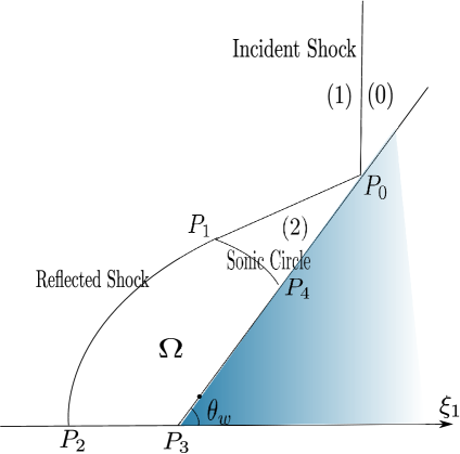
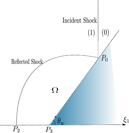
When $u_{1}>c_{1}$, besides the configurations shown in Figs. 7.2–7.2, there is an additional possibility that the reflected-diffracted shock is attached to the wedge vertex $P_{3}$, i.e., $P_{2}=P_{3}$; see Figs. 7.4–7.4.

Figure 7.3: Attached supersonic regular reflection

Figure 7.4: Attached subsonic regular reflection

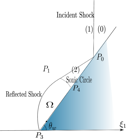
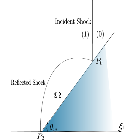
The regular reflection problem is posed in the region:

$$\Lambda=\mathbb{R}^{2}_{+}\setminus\{\bm{\xi}\;:\;\xi_{1}>0,0<\xi_{2}<\xi_{1}\tan\theta_{\rm w}\},$$

where $\mathbb{R}^{2}_{+}:=\mathbb{R}^{2}\cap\{\xi_{1}>0\}$.

Definition 7.1.

$\varphi\in C^{0,1}(\overline{\Lambda})$ is a weak solution of the shock reflection-diffraction problem if $\varphi$ satisfies equation (2.5) in $\Lambda$, the boundary conditions:

$$\partial_{\bm{\nu}}\varphi=0\qquad\mbox{on $\partial\Lambda$}$$ (7.3)

in the weak sense (defined below), and the asymptotic conditions:

$$\lim_{R\to\infty}\|\varphi-\overline{\varphi}\|_{0,\Lambda\setminus B_{R}(\mathbf{0})}=0,$$ (7.4)

where

$$\bar{\varphi}=\begin{cases}\varphi_{0}\qquad\mbox{for $\xi_{1}>\xi_{1}^{0},\,\,\,\xi_{2}>\xi_{1}\tan\theta_{\rm w}$},\\[2.84526pt] \varphi_{1}\qquad\mbox{for $\xi_{1}<\xi_{1}^{0},\,\,\,\xi_{2}>0$},\end{cases}$$

and $\xi_{1}^{0}>0$ is the location of the incident shock $S_{0}$.

In Definition 7.1, the solution is understood in the following weak sense: We consider solutions with a positive lower bound for the density, so that (7.3) is equivalent to the conormal condition:

$$\rho(|D\varphi|^{2},\varphi)\partial_{\bm{\nu}}\varphi=0.$$

Thus, a weak solution of problem (2.5) and (7.3) is given by Definition 2.1 in region $\Lambda$, with the following change: (2.11) is satisfied for any $\zeta\in C^{\infty}_{c}(\mathbb{R}^{2})$ (whose support does not have to be in $\Lambda$).

Next, we define the points and lines on Figs. 7.2–7.2. The incident shock is line $S_{0}:=\{\xi_{1}=\xi_{1}^{0}\}$ with $\xi_{1}^{0}=\frac{\rho_{1}u_{1}}{\rho_{1}-\rho_{0}}>0$. The center, $O_{2}=(u_{2},v_{2})$, of the sonic circle $B_{c_{2}}(O_{2})$ of state $(2)$ lies on the wedge boundary between the reflection point $P_{0}$ and the wedge vertex $P_{3}$ for both the supersonic and subsonic cases.

Then, for the supersonic case, i.e., when $|D\varphi_{2}(P_{0})|=|P_{0}O_{2}|>c_{2}$ with $P_{0}\notin\overline{B_{c_{2}}(O_{2})}$, we denote by $P_{4}$ the upper point of intersection of $\partial B_{c_{2}}(O_{2})$ with the wedge boundary so that $O_{2}\in P_{3}P_{4}$. Also, $\partial B_{c_{2}}(O_{2})$ of state $(2)$ intersects line $S_{1}$, and one of the points of intersection, $P_{1}\in\Lambda$, is such that segment $P_{0}P_{1}$ is outside $B_{c_{2}}(O_{2})$. We denote the arc of $\partial B_{c_{2}}(O_{2})$ by $\Gamma_{\text{\rm sonic}}=P_{1}P_{4}$. The curved part of the reflected-diffracted shock is $\Gamma_{\text{\rm shock}}=P_{1}P_{2}$, where $P_{2}\in\{\xi_{2}=0\}$. Denote the line segments $\Gamma_{\rm sym}:=P_{2}P_{3}$ and $\Gamma_{\text{\rm wedge}}:=P_{3}P_{4}$. The lines and curves $\Gamma_{\text{\rm shock}}$, $\Gamma_{\text{\rm sonic}}$, $\Gamma_{\rm sym}$, and $\Gamma_{\text{\rm wedge}}$ do not have common points, except their endpoints $P_{1}$, …, $P_{4}$. Thus, $\Gamma_{\text{\rm shock}}\cup\Gamma_{\text{\rm sonic}}\cup\Gamma_{\rm sym}\cup\Gamma_{\text{\rm wedge}}$ is a closed curve without self-intersection. Denote by $\Omega$ the domain bounded by this curve.

For the subsonic/sonic case, i.e., when $|D\varphi_{2}(P_{0})|=|P_{0}O_{2}|\leq c_{2}$ so that $P_{0}\in\overline{B_{c_{2}}(O_{2})}$, the curved reflected-diffracted shock is $\Gamma_{\text{\rm shock}}=P_{0}P_{2}$ that does not have common interior points with the line segments $\Gamma_{\rm sym}=P_{2}P_{3}$ and $\Gamma_{\text{\rm wedge}}=P_{0}P_{3}$. Then $\Gamma_{\text{\rm shock}}\cup\Gamma_{\rm sym}\cup\Gamma_{\text{\rm wedge}}$ is a closed curve without self-intersection, and $\Omega$ is the domain bounded by this curve.

Furthermore, in some parts of the argument below, it is convenient to extend problem (2.5) and (7.3), given in $\Lambda$ by even reflection about the $\xi_{1}$–axis, i.e., defining $\varphi^{\rm ext}(-\xi_{1},\xi_{2}):=\varphi(\xi_{1},\xi_{2})$ for any $\bm{\xi}=(\xi_{1},\xi_{2})\in\Lambda$. Then $\varphi^{\rm ext}$ is defined in region $\Lambda^{\rm ext}$ obtained from $\Lambda$ by adding the reflected region $\Lambda^{-}$, i.e., $\Lambda^{\rm ext}=\Lambda\cup\{(\xi_{1},0)\;:\;\xi_{1}<0\}\cup\Lambda^{-}$. In a similar way, region $\Omega$ and curve $\Gamma_{\text{\rm shock}}\subset\partial\Omega$ can be extended into the corresponding region $\Omega^{\rm ext}$ and curve $\Gamma_{\text{\rm shock}}^{\rm ext}\subset\partial\Omega^{\rm ext}$.

Now we define a class of solutions, with structure as shown on Figs. 7.2–7.2.

Definition 7.2.

Let $\theta_{\rm w}\in(\theta_{\rm w}^{\rm d},\frac{\pi}{2})$. A function $\varphi\in C^{0,1}(\overline{\Lambda})$ is an admissible solution of the regular reflection problem (2.5) and (7.3)–(7.4) if $\varphi$ is a solution in the sense of Definition 7.1 and satisfies the following properties:

1. The structure of solutions is as follows:

   • If $|D\varphi_{2}(P_{0})|>c_{2}$, then $\varphi$ is of the supersonic regular shock reflection-diffraction configuration shown on Fig. 7.2 and satisfies:

     The reflected-diffracted shock $\Gamma_{\text{\rm shock}}$ is $C^{2}$ in its relative interior. Curves $\Gamma_{\text{\rm shock}}$, $\Gamma_{\text{\rm sonic}}$, $\Gamma_{\text{\rm wedge}}$, and $\Gamma_{\rm sym}$ do not have common points except their endpoints.

     $\varphi$ satisfies the following properties:

     $$\varphi\in C^{0,1}(\Lambda)\cap C^{1}(\Lambda\setminus(S_{0}\cup\overline{P_{0}P_{1}P_{2}})),$$

     $$\varphi\in C^{1}(\overline{\Omega})\cap C^{3}(\overline{\Omega}\setminus(\overline{\Gamma}_{\text{\rm sonic}}\cup\{P_{2},\,P_{3}\})),$$

     $$\varphi=\left\{\begin{array}[]{ll}\varphi_{0}\qquad\mbox{for $\xi_{1}>\xi_{1}^{0}$ and $\xi_{2}>\xi_{1}\tan\theta_{\rm w}$},\\[5.69054pt] \varphi_{1}\qquad\mbox{for $\xi_{1}<\xi_{1}^{0}$ and above curve $P_{0}P_{1}P_{2}$},\\[5.69054pt] \varphi_{2}\qquad\mbox{in region $P_{0}P_{1}P_{4}$}.\end{array}\right.$$ (7.8)

   • If $|D\varphi_{2}(P_{0})|\leq c_{2}$, then $\varphi$ is of the subsonic regular shock reflection-diffraction configuration shown on Fig. 7.2 and satisfies:

     The reflected-diffracted shock $\Gamma_{\text{\rm shock}}$ is $C^{2}$ in its relative interior. Curves $\Gamma_{\text{\rm shock}}$, $\Gamma_{\text{\rm wedge}}$, and $\Gamma_{\rm sym}$ do not have common points except their endpoints.

     $\varphi$ satisfies the following properties:

     $$\varphi\in C^{0,1}(\Lambda)\cap C^{1}(\Lambda\setminus\overline{\Gamma}_{\text{\rm shock}}),$$

     $$\varphi\in C^{1}(\overline{\Omega})\cap C^{3}(\overline{\Omega}\setminus\{P_{0},P_{2},P_{3}\}),$$

     $$\varphi=\left\{\begin{array}[]{ll}\varphi_{0}&\mbox{for $\xi_{1}>\xi_{1}^{0}$ and $\xi_{2}>\xi_{1}\tan\theta_{\rm w}$},\\[5.69054pt] \varphi_{1}&\mbox{for $\xi_{1}<\xi_{1}^{0}$ and above curve $P_{0}P_{2}$},\\[5.69054pt] \varphi_{2}(P_{0})&\mbox{at $P_{0}$},\end{array}\right.$$ (7.12)

     $$D\varphi(P_{0})=D\varphi_{2}(P_{0}).$$

   Furthermore, in both supersonic and subsonic cases,

   $$\Gamma_{\text{\rm shock}}^{\rm ext}\,\,\,\,\mbox{is $C^{1}$ in its relative interior}.$$ (7.13)

2. Equation (2.5) is strictly elliptic in $\overline{\Omega}\setminus\,\overline{\Gamma_{\text{\rm sonic}}}$:

   $$|D\varphi|<c(|D\varphi|^{2},\varphi)\qquad\mbox{ in $\overline{\Omega}\setminus\,\overline{\Gamma_{\text{\rm sonic}}}$},$$

   where, for the subsonic and sonic cases, we have used notation $\overline{\Gamma_{\text{\rm sonic}}}=\{P_{0}\}$.

3. $\partial_{\bm{\nu}}\varphi_{1}>\partial_{\bm{\nu}}\varphi>0$ on $\Gamma_{\text{\rm shock}}$, where $\bm{\nu}$ is the normal vector to $\Gamma_{\text{\rm shock}}$ pointing into $\Omega$.

4. $\varphi_{2}\leq\varphi\leq\varphi_{1}$ in $\Omega$.

5. Let $\mathbf{e}_{S_{1}}$ be the unit vector parallel to $S_{1}:=\{\varphi_{1}=\varphi_{2}\}$, oriented so that $\mathbf{e}_{S_{1}}\cdot D\varphi_{2}(P_{0})>0$:

   $$\mathbf{e}_{S_{1}}=-\frac{(v_{2},\,u_{1}-u_{2})}{\sqrt{(u_{1}-u_{2})^{2}+v_{2}^{2}}}.$$ (7.14)

   Let $\mathbf{e}_{\xi_{2}}=(0,1)$. Then

   $$\partial_{\mathbf{e}_{S_{1}}}(\varphi_{1}-\varphi)\leq 0,\quad\,\,\partial_{\xi_{2}}(\varphi_{1}-\varphi)\leq 0\qquad\;\;\mbox{ on $\Gamma_{\text{\rm shock}}$}.$$ (7.15)

Below we continue to use the notational convention:

$$\mbox{$\overline{\Gamma_{\text{\rm sonic}}}:=\{P_{0}\}$, $\;P_{1}:=P_{0}$, $P_{4}:=P_{0}$ $\quad$ for the subsonic and sonic cases}.$$ (7.16)

Remark 7.3.

Since the admissible solution $\varphi$ in Definition 7.2 is a weak solution in the sense of Definition 7.1 and has the regularity as in Definition 7.2(i), it satisfies (2.16) classically in $\Omega$ with $\phi=\varphi-\varphi_{1}$, the Rankine-Hugoniot conditions:

$$\varphi=\varphi_{1},\quad\rho(|D\varphi|^{2},\varphi)D\varphi\cdot\bm{\nu}=\rho_{1}D\varphi_{1}\cdot\bm{\nu}\qquad\mbox{ on $\Gamma_{\text{\rm shock}}$},$$ (7.17)

and the boundary conditions:

$$\partial_{\bm{\nu}}\varphi=0\qquad\;\mbox{ on $\Gamma_{\text{\rm wedge}}\cup\Gamma_{\rm sym}$}.$$ (7.18)

Note also that, rewriting (7.18) in terms of $\phi=\varphi-\varphi_{1}$, we have

$$\begin{split}&\partial_{\bm{\nu}}\phi=-u_{1}\sin\theta_{\rm w}\qquad\;\mbox{ on $\Gamma_{\text{\rm wedge}}$},\\ &\partial_{\bm{\nu}}\phi=0\qquad\qquad\qquad\,\mbox{ on $\Gamma_{\rm sym}$}.\end{split}$$ (7.19)

Remark 7.4.

An admissible solution $\varphi$ is not a constant state in $\Omega$ $($recall that $\theta_{\rm w}<\frac{\pi}{2}$). Indeed, if $\varphi$ is a constant state in $\Omega$, then $\varphi=\varphi_{2}$ in $\Omega$: This follows from (7.8) for the supersonic case since $\varphi$ is $C^{1}$ across $\Gamma_{\text{\rm sonic}}$, and from the property that $(\varphi,D\varphi)=(\varphi_{2},D\varphi_{2})$ at $P_{0}$ for the subsonic case. However, $\varphi_{2}$ does not satisfy (7.18) on $\Gamma_{\rm sym}$ since $\mathbf{v}_{2}=(u_{2},v_{2})=(u_{2},u_{2}\tan\theta_{\rm w})$ with $u_{2}>0$ and $\theta_{\rm w}\in(0,\frac{\pi}{2})$.

Remark 7.5.

Let $\varphi$ be an admissible solution and $\phi:=\varphi-\varphi_{1}$. For a unit vector $\mathbf{e}\in\mathbb{R}^{2}$, denote

$$w=\phi_{\mathbf{e}}.$$

Then, from the regularity in Definition 7.2(i),

$$w\in C(\overline{\Omega})\cap C^{2}(\overline{\Omega}\setminus(\overline{\Gamma}_{\text{\rm sonic}}\cup\{P_{3}\})),$$

where we have used (7.16) for the subsonic and sonic cases.

We first notice that $w$ satisfies equation (3.2) in the $(S,T)$–coordinates with basis $\{\mathbf{e},\mathbf{e}^{\perp}\}$. Equation (3.2) has the same coefficients of the second-order terms as equation (2.6), so that (3.2) is strictly elliptic in $\overline{\Omega}\setminus\,\overline{\Gamma_{\text{\rm sonic}}}$ by Definition 7.2(ii).

Furthermore, by (cf-book2014shockreflection, , Lemma 5.1.3), $w$ satisfies the following boundary conditions on the straight segments $\Gamma_{\text{\rm wedge}}$ and $\Gamma_{\rm sym}$: If $\mathbf{e}\cdot\bm{\tau}\neq 0$ for a unit tangent vector $\bm{\tau}$ on $\Gamma_{\text{\rm wedge}}$ (resp. $\Gamma_{\rm sym}$), then

$$w_{\bm{\nu}}+\frac{(\mathbf{e}\cdot\bm{\nu})(c^{2}-\varphi_{\bm{\tau}}^{2})}{(\mathbf{e}\cdot\bm{\tau})(c^{2}-\varphi_{\bm{\nu}}^{2})}w_{\bm{\tau}}=0\qquad\mbox{on $\Gamma_{\text{\rm wedge}}^{0}$ {\rm(}resp. $\Gamma_{\rm sym}^{0}${\rm)}}.$$ (7.20)

The coefficients are continuous and hence locally bounded, which implies that these boundary conditions are oblique on $\Gamma_{\text{\rm wedge}}^{0}$ (resp. $\Gamma_{\rm sym}^{0}$).

Lemma 7.6.

Definition 7.2 is equivalent to the definition of admissible solutions in cf-book2014shockreflection ; see Definitions 15.1.1–15.1.2 there.

Proof.

In order to show that the solutions in Definition 7.2 satisfy all the properties in Definitions 15.1.1–15.1.2 of Chen-Feldman cf-book2014shockreflection , it requires to show that they satisfy:

$$\xi_{1P_{2}}\leq\xi_{1P_{1}},\quad\,\,\overline{\Gamma_{\text{\rm shock}}}\subset(\Lambda\setminus\overline{B_{c_{1}}(O_{1})})\cap\{\xi_{1P_{2}}\leq\xi_{1}\leq\xi_{1P_{1}}\},$$ (7.21)

$$\partial_{\mathbf{e}_{S_{1}}}(\varphi_{1}-\varphi)\leq 0,\quad\partial_{\xi_{2}}(\varphi_{1}-\varphi)\leq 0\qquad\;\;\mbox{in $\overline{\Omega}$},$$ (7.22)

where $O_{1}=(u_{1},0)$ is the center of sonic circle of state (1) and, in the subsonic reflection case (see Fig. 7.2), we have used the notational convention (7.16). Moreover, note that the inequalities in (7.15) hold on $\Gamma_{\text{\rm shock}}$, while these inequalities in (7.22) hold in the larger domain $\overline{\Omega}$.

We first show both (7.22) and the stronger property:

$$\partial_{\mathbf{e}_{S_{1}}}(\varphi_{1}-\varphi)<0,\quad\,\,\partial_{\xi_{2}}(\varphi_{1}-\varphi)<0\qquad\;\;\mbox{ in $\Omega$}.$$ (7.23)

The argument is the same as the one in the proof of Remark 2.5 (see §6) for $\phi=\varphi-\varphi_{1}$ in the present case. We only need to check for $\mathbf{e}=\mathbf{e}_{S_{1}}$ and $\mathbf{e}=\mathbf{e}_{\xi_{2}}$ that, for any point $\bm{\xi}\in\partial\Omega\setminus\Gamma_{\text{\rm shock}}^{0}$, $\phi_{\mathbf{e}}$ satisfies that

either $$\phi_{\mathbf{e}}(\bm{\xi})\geq 0 \phi_{\mathbf{e}} \bm{\xi}$$ or cannot attain its local minimum at . (7.24)

Note that $\partial\Omega\setminus\Gamma_{\text{\rm shock}}^{0}=\overline{\Gamma_{\text{\rm sonic}}}\cup\Gamma_{\text{\rm wedge}}\cup\Gamma_{\rm symm}\cup\{P_{3}\}$.

Consider first $\mathbf{e}=\mathbf{e}_{S_{1}}$. Since $D\varphi(P_{3})=(0,0)$ by (7.18) and $\varphi\in C^{1}(\overline{\Omega})$, we conclude that $w(P_{3})=0$. Next, $\mathbf{e}_{S_{1}}\cdot\bm{\tau}\neq 0$ on $\Gamma_{\text{\rm wedge}}\cup\Gamma_{\rm sym}$ by (cf-book2014shockreflection, , Lemma 7.5.12). Then, by Remark 7.5, $\phi_{\mathbf{e}}$ satisfies a homogeneous elliptic equation in $\Omega$ and the oblique boundary conditions (7.20) on $\Gamma_{\text{\rm wedge}}^{0}\cup\Gamma_{\rm sym}^{0}$, so that $w$ cannot attain its local minimum on $\Gamma_{\text{\rm wedge}}^{0}\cup\Gamma_{\rm sym}^{0}$, unless $w$ is constant in $\Omega$ in which case $w\equiv w(P_{3})=0$ in $\overline{\Omega}$. On $\overline{\Gamma}_{\text{\rm sonic}}$, $(\varphi,D\varphi)=(\varphi_{2},D\varphi_{2})$ as shown in Remark 7.4, where we have used notation (7.16). Also, $\mathbf{e}_{S_{1}}\cdot D(\varphi_{2}-\varphi_{1})=0$ by (7.14). Thus, $\phi_{\mathbf{e}_{S_{1}}}=\mathbf{e}_{S_{1}}\cdot D(\varphi_{2}-\varphi_{1})=0$ on $\overline{\Gamma}_{\text{\rm sonic}}$, which implies (7.24) for $\mathbf{e}=\mathbf{e}_{S_{1}}$.

Now we show (7.24) for $\mathbf{e}=\mathbf{e}_{\xi_{2}}$, i.e., $w=\phi_{\xi_{2}}$. The argument is similar to the previous case, with the following differences: First, $\mathbf{e}_{\xi_{2}}\cdot\bm{\tau}=0$ on $\Gamma_{\rm sym}$ so that, instead of (7.20), we obtain that $w=0$ on $\Gamma_{\rm sym}$ by (7.19). Also, on $\Gamma_{\text{\rm sonic}}$, we use again that $D\varphi=D\varphi_{2}$ to obtain that $w=\phi_{\xi_{2}}=(\varphi_{2}-\varphi_{1})_{\xi_{2}}=v_{2}\geq 0$. The rest of the argument is the same as above, which leads to (7.24) for $\mathbf{e}=\mathbf{e}_{\xi_{2}}$.

Repeating the proof of Remark 2.5 (see §6), in which $\phi$ is not a constant state by Remark 7.4, we obtain (7.23). With this, (7.22) is proved.

Next we show (7.21). Since $\overline{\Gamma_{\text{\rm shock}}}\subset\Lambda\setminus\overline{B_{c_{1}}(O_{1})}$, then $\varphi_{1}$ is supersonic on $\Gamma_{\text{\rm shock}}$. This is a standard consequence of the Rankine-Hugoniot conditions (7.17), combined with the entropy condition of Definition 7.2(iii).

It remains to show that $\xi_{1P_{2}}\leq\xi_{1P_{1}}$ and $\overline{\Gamma_{\text{\rm shock}}}\subset\{\xi_{1P_{2}}\leq\xi_{1}\leq\xi_{1P_{1}}\}$. From (7.23), $\phi_{\xi_{2}}>0$ in $\Omega$. Also, $\phi=0$ on $\Gamma_{\text{\rm shock}}$ and $\phi\leq 0$ in $\Omega$ by (iv). From these properties and the regularity of curve $\Gamma_{\text{\rm shock}}$, it follows that any vertical line that has a non-empty intersection with $\Gamma_{\text{\rm shock}}$ intersects $\Gamma_{\text{\rm shock}}$ either at one point or on a closed interval. Moreover,

If $$(\xi_{1}^{*},\xi_{2}^{*})\in\Gamma_{\text{\rm shock}} \Omega\cap\{(\xi_{1},\xi_{2})\;:\;\xi_{1}=\xi_{1}^{*}\}\subset\{(\xi_{1},\xi_{2})\;:\;\xi_{2}<\xi_{2}^{*}\}$$, then . (7.25)

From these properties, we conclude that

$$\overline{\Gamma}_{\text{\rm shock}}\subset\{\min(\xi_{1P_{1}},\,\xi_{1P_{2}})\leq\xi_{1}\leq\max(\xi_{1P_{1}},\,\xi_{1P_{2}})\}.$$

It remains to show that $\xi_{1P_{2}}\leq\xi_{1P_{1}}$. Assume that $\xi_{1P_{2}}>\xi_{1P_{1}}$. Then, from (7.25) and the structure of $\Omega$ described in Definition 7.2(i), we conclude that $\overline{\Gamma}_{\text{\rm shock}}$ is contained within the following subregion of $\{\xi_{1P_{1}}\leq\xi_{1}\leq\xi_{1P_{2}}\}$: Above $\overline{\Gamma}_{\text{\rm sonic}}$ on $\{\xi_{1P_{1}}\leq\xi_{1}\leq\min(\xi_{1P_{2}},\xi_{1P_{4}})\}$, and above $\Gamma_{\text{\rm wedge}}$ on $\{\xi_{1P_{4}}\leq\xi_{1}\leq\xi_{1P_{2}}\}$ if $\xi_{1P_{2}}\geq\xi_{1P_{4}}$. This implies that $\overline{\Gamma}_{\text{\rm shock}}\subset\{\xi_{2}>0\}$. This contradicts the fact that endpoint $P_{2}$ of $\Gamma_{\text{\rm shock}}$ lies on $\{\xi_{2}=0\}$. Now (7.21) is proved.

Therefore, we have shown that the solutions in Definition 7.2 satisfy all the properties in Definitions 15.1.1–15.1.2 of cf-book2014shockreflection .

Now we show that the admissible solutions defined in Definitions 15.1.1–15.1.2 of cf-book2014shockreflection satisfy all the properties of Definition 7.2. For that, we need to show that the admissible solutions in Definitions 15.1.1–15.1.2 of cf-book2014shockreflection satisfy property (iii) of Definition 7.2. This is proved in (cf-book2014shockreflection, , Lemma 8.1.7 and Proposition 15.2.1). ∎

From Lemma 7.6, all the estimates and properties of admissible solutions shown in cf-book2014shockreflection hold for the admissible solutions defined above. We list some of these properties in the following theorem.

Below we use the notation that, for two unit vectors $\mathbf{e},{\mathbf{f}}\in\mathbb{R}^{2}$ with $\mathbf{e}\neq\pm{\mathbf{f}}$,

$$Con(\mathbf{e},\mathbf{f}):=\{a\mathbf{e}+b\mathbf{f}\;:\;a,b>0\}.$$ (7.26)

Theorem 7.1 (Properties of admissible solutions).

   There exits a constant $\alpha=\alpha(\rho_{0},\rho_{1},\gamma)\in(0,\frac{1}{2})$ such that any admissible solution in the sense of Definition 7.2 with wedge angle $\theta_{\rm w}\in(\theta_{\rm w}^{\rm d},\frac{\pi}{2})$ has the following properties:

1. Additional regularity:

   • If $|D\varphi_{2}(P_{0})|>c_{2}$, i.e., when $\varphi$ is of the supersonic regular shock reflection-diffraction configuration as in Fig. 7.2, it satisfies

     $$\varphi\in C^{\infty}(\overline{\Omega}\backslash(\overline{\Gamma_{\text{\rm sonic}}}\cup\{P_{3}\}))\cap C^{1,1}(\overline{\Omega}\backslash\{P_{3}\})\cap C^{1,\alpha}(\overline{\Omega}).$$

     The reflected-diffracted shock $P_{0}P_{1}P_{2}$ $($where $P_{0}P_{1}$ is the straight segment and $P_{1}P_{2}=\Gamma_{\text{\rm shock}}$) is $C^{2,\beta}$ up to its endpoints for any $\beta\in[0,\frac{1}{2})$ and $C^{\infty}$ except $P_{1}$.

   • If $|D\varphi_{2}(P_{0})|\leq c_{2}$, i.e., when $\varphi$ is of the subsonic regular shock reflection-diffraction configuration as in Fig. 7.2, it satisfies

     $$\varphi\in C^{1,\beta}(\overline{\Omega})\cap C^{1,\alpha}(\overline{\Omega}\setminus\{P_{0}\})\cap C^{\infty}(\overline{\Omega}\setminus\{P_{0},P_{3}\})$$

     for some $\beta=\beta(\rho_{0},\rho_{1},\gamma,\theta_{\rm w})\in(0,\alpha]$ which is non-decreasing with respect to $\theta_{\rm w}$, and the reflected-diffracted shock $\Gamma_{\text{\rm shock}}$ is $C^{1,\beta}$ up to its endpoints and $C^{\infty}$ except $P_{0}$.

   Furthermore, in both supersonic and subsonic cases,

   $$\varphi^{\rm ext}\in C^{\infty}(\Omega^{\rm ext}\cup(\Gamma_{\text{\rm shock}}^{\rm ext})^{0}).$$

2. For each $\mathbf{e}\in Con(\mathbf{e}_{S_{1}},\mathbf{e}_{\xi_{2}})$,

   $$\partial_{\mathbf{e}}(\varphi_{1}-\varphi)<0\qquad\mbox{in $\overline{\Omega}$},$$ (7.27)

   where vectors $\mathbf{e}_{S_{1}}$ and $\mathbf{e}_{\xi_{2}}$ are introduced in Definition 7.2(v).

3. Denote by $\bm{\nu}_{\rm w}$ the unit interior normal vector to $\Gamma_{\text{\rm wedge}}$ (pointing into $\Omega$), i.e., $\bm{\nu}_{\rm w}=(-\sin\theta_{\rm w},\cos\theta_{\rm w})$. Then $\partial_{\bm{\nu}_{\rm w}}(\varphi-\varphi_{2})\leq 0$ in $\overline{\Omega}$.

Proof.

Below we use the equivalence shown in Lemma 7.6.

Assertion (i) follows from Definition 7.2(i) and (cf-book2014shockreflection, , Corollary 11.4.7, Proposition 11.5.1, Corollary 16.6.12). Assertion (ii) is obtained in (cf-book2014shockreflection, , Corollary 8.2.10, Proposition 15.2.1). Assertion (iii) follows from (cf-book2014shockreflection, , Lemma 8.2.19, Proposition 15.2.1), where ${\mathbf{n}}_{\rm w}=-\bm{\nu}_{\rm w}$. ∎

Remark 7.7.

We note that $\bm{\nu}_{\rm w}\in Con(\mathbf{e}_{S_{1}},\mathbf{e}_{\xi_{2}})$ for any wedge angle $\theta_{\rm w}\in(\theta_{\rm w}^{\rm d},\frac{\pi}{2})$, which is proved in (cf-book2014shockreflection, , Lemma 8.2.11).

Now we state the results on the existence of admissible solutions.

Theorem 7.2 (Global solutions up to the detachment angle for the case: $u_{1}\leq c_{1}$).

Let the initial data $(\rho_{0},\rho_{1},\gamma)$ satisfy that $u_{1}\leq c_{1}$. Then, for each $\theta_{\rm w}\in(\theta_{\rm w}^{\rm d},\frac{\pi}{2})$, there exists an admissible solution of the regular reflection problem in the sense of Definition 7.2, which satisfies the properties stated in Theorem 7.1.

Proof.

The existence of admissible solutions directly follows from Lemma 7.6 and (cf-book2014shockreflection, , Theorem 2.6.7 and Remark 2.6.8). ∎

When $u_{1}>c_{1}$, the results of Theorem 7.2 hold for any wedge angle $\theta_{\rm w}$ from $\frac{\pi}{2}$ until either $\theta_{\rm w}^{\rm d}$ or $\theta_{\rm w}^{\rm c}\in(\theta_{\rm w}^{\rm d},\frac{\pi}{2})$ when the shock hits the wedge vertex ${P_{3}}$.

Theorem 7.3 (Global solutions up to the detachment angle for the case: $u_{1}>c_{1}$).

Let the initial data $(\rho_{0},\rho_{1},\gamma)$ satisfy that $u_{1}>c_{1}$. Then there is $\theta_{\rm w}^{\rm c}\in[\theta^{\rm d}_{\rm w},\frac{\pi}{2})$ such that, for each $\theta_{\rm w}\in(\theta_{\rm w}^{\rm c},\frac{\pi}{2})$, there exists an admissible solution of the regular reflection problem in the sense of Definition 7.2, which satisfies the properties stated in Theorem 7.1.

If $\theta_{\rm w}^{\rm c}>\theta^{\rm d}_{\rm w}$, then, for the wedge angle $\theta_{\rm w}=\theta_{\rm w}^{\rm c}$, there exists an attached shock solution $\varphi$ with all the properties listed in Definition 7.2 and Theorem 7.1(ii)–(iii) except that $P_{3}=P_{2}$ $($we denote $P_{3}$ for that point below$)$. In addition, for the regularity of solution $\varphi$, we have

• For the supersonic case with $\theta_{\rm w}=\theta^{\rm c}_{\rm w}$,

  $$\varphi\in C^{\infty}(\overline{\Omega}\backslash(\overline{\Gamma_{\text{\rm sonic}}}\cup\{P_{3}\}))\cap C^{1,1}(\overline{\Omega}\backslash\{P_{3}\})\cap C^{0,1}(\overline{\Omega}),$$

  and the reflected shock $P_{0}P_{1}P_{3}$ is Lipschitz up to the endpoints, $C^{2,\beta}$ for any $\beta\in[0,\frac{1}{2})$ except point $P_{3}$, and $C^{\infty}$ except points $P_{1}$ and $P_{3}$.

• For the subsonic case with $\theta_{\rm w}=\theta^{\rm c}_{\rm w}$,

  $$\varphi\in C^{\infty}(\overline{\Omega}\backslash\{P_{0},\,P_{3}\})\cap C^{1,\beta}(\overline{\Omega}\backslash\{P_{3}\})\cap C^{0,1}(\overline{\Omega})$$

  for $\beta$ as in Theorem 7.1, and the reflected shock $P_{0}P_{3}$ is Lipschitz up to the endpoints, $C^{1,\beta}$ except point $P_{3}$, and $C^{\infty}$ except points $P_{0}$ and $P_{3}$.

Proof.

The existence of admissible solutions directly follows from Lemma 7.6 and (cf-book2014shockreflection, , Theorem 2.6.9 and Remark 2.6.8), where we note that (cf-book2014shockreflection, , Remark 2.6.8) applies to the case: $u_{1}>c_{1}$ as well, although this is not stated explicitly. ∎

Now we show that the admissible solutions satisfy the conditions of Theorems 2.1–2.3.

Lemma 7.8.

The following statements hold:

1. Any admissible solution in the sense of Definition 7.2 satisfies the conditions of Theorems 2.1 and 2.3.

2. Any regular reflection-diffraction solution in the sense of Definition 7.1 with properties (i)–(iv) of Definition 7.2 and with shock $\Gamma_{\text{\rm shock}}$ being a strictly convex graph in the sense of (2.18)–(2.19) satisfies property (v) of Definition 7.2.

Proof.

We divide the proof into seven steps: Assertion (i) is proved in Steps 1–6, while assertion (ii) is proved in Step 7.

1. We use $\Lambda^{\rm ext}$, $\Gamma_{\text{\rm shock}}^{\rm ext}$, and $\varphi^{\rm ext}$ defined before Definition 7.2. Combining the structure of equation (2.5) with the boundary conditions (7.3) on the negative $\xi_{1}$–axis yields that the reflected/extended function $\varphi^{\rm ext}$ is a weak solution of equation (2.5) in $\Lambda^{\rm ext}$. By the boundary conditions (7.3), state $(1)$ satisfies $\partial_{\bm{\nu}}\varphi_{1}=0$ on the $\xi_{1}$–axis. Then the structure of the constant state (see §2.1) implies that $\varphi_{1}(-\xi_{1},\xi_{2})=\varphi_{1}(\xi_{1},\xi_{2})$ in $\mathbb{R}^{2}$ so that $\varphi_{1}^{\rm ext}=\varphi_{1}$. We also note the regularity of $\varphi^{\rm ext}$ in Theorem 7.1(i). Thus, the extended shock $\Gamma_{\text{\rm shock}}^{\rm ext}$ separates the constant state $\varphi_{1}$ from the smooth solution $\varphi^{\rm ext}$ of equation (2.5) in $\Omega^{\rm ext}$, and the Rankine-Hugoniot conditions (7.17) are satisfied for $\varphi^{\rm ext}$ and $\varphi_{1}$ on $\Gamma_{\text{\rm shock}}^{\rm ext}$.

2. Region $\Omega$ satisfies the conditions in Framework (A). Indeed, for the supersonic reflection case (see Fig. 7.2), the required piecewise-regularity holds, since $\Gamma_{\text{\rm wedge}}$ and $\Gamma_{\rm sym}$ are straight segments, $\Gamma_{\text{\rm sonic}}$ is an arc of circle, and $\Gamma_{\text{\rm shock}}$ has the regularity stated in Theorem 7.1(i). The fact that all the angles of the corners of $\Omega$ are less than $\pi$ is verified as follows:

Consider first the supersonic case. Since curve $P_{0}P_{1}P_{2}$ is $C^{2}$ at $P_{1}$, and $P_{0}P_{1}$ is a straight segment, we use that the center of sonic circle of state $(2)$ is on $\Gamma^{0}_{\rm wedge}$ and $P_{0}$ is outside that circle to conclude that the angle at $P_{1}$ is between $(\frac{\pi}{2},\pi)$, and the angle at $P_{4}$ is $\frac{\pi}{2}$. Also, since (7.13) shows that $\Gamma_{\text{\rm shock}}^{\rm ext}$ is smooth near $P_{2}$, it follows that the interior angle to $\Omega$ at $P_{2}$ is $\frac{\pi}{2}$. Finally, the angle at $P_{3}$ is $\pi-\theta\in(\frac{\pi}{2},\pi)$.

For the subsonic reflection case, the angles at $P_{2}$ and $P_{3}$ are handled similarly. The angle at $P_{0}$ is in $(0,\frac{\pi}{2})$ for the following reason: By (cf-book2014shockreflection, , Lemma 8.2.11, Proposition 15.2.1), for any $\theta_{\rm w}\in(\theta_{\rm w}^{\rm d},\frac{\pi}{2})$, $\bm{\nu}_{\rm w}\in Con(\mathbf{e}_{S_{1}},\mathbf{e}_{\xi_{2}})$ so that, using the regularity of $\Gamma_{\text{\rm shock}}$ in Theorem 7.2(i), property (iii) in Theorem 7.2, and $\varphi=\varphi_{1}$ on $\Gamma_{\text{\rm shock}}$, we conclude that $\Gamma_{\text{\rm shock}}$ is a graph:

$$\Gamma_{\text{\rm shock}}=\{(f(T),T)\;:\;T_{P_{2}}\leq T\leq T_{P_{0}}\}$$

of a function $f(T)\in C^{2}([T_{P_{2}},T_{P_{0}}))\cap C^{1,\beta}([T_{P_{2}},T_{P_{0}}])$, where the $(S,T)$–coordinates are along the normal and tangent directions to $\Gamma_{\text{\rm wedge}}$.

3. The entropy condition (A1) of Theorem 2.1 follows directly from property (iii) of Definition 7.2, where state $(0)$ in Theorem 2.1 is state $(1)$ in the regular shock reflection problem.

From the regularity of $\varphi$ and $\Gamma_{\text{\rm shock}}$ in Theorem 7.1(i), we see that conditions (A2) and (A4) of Theorem 2.1 hold.

Property (ii) of Definition 7.2 implies that condition (A3) of Theorem 2.1 holds.

4. Using the notations of the endpoints of $\Gamma_{\text{\rm shock}}$ as in Framework (A) by $A:={P_{1}}$ and $B:=P_{2}$, we see from the properties of Definition 7.2(i) that

$$\bm{\tau}_{A}=\mathbf{e}_{S_{1}},\qquad\bm{\tau}_{B}=\mathbf{e}_{\xi_{2}}.$$

As we discussed in Step 2, $\Gamma_{\text{\rm shock}}$ is orthogonal to the $\xi_{1}$–axis at $P_{2}$. From this and (cf-book2014shockreflection, , Lemma 7.5.12), $\mathbf{e}_{\xi_{1}}\neq\pm\mathbf{e}_{S_{1}}$. Also, combining property (ii) of Theorem 7.1 with the fact that $\Gamma_{\text{\rm shock}}$ is the level set $\varphi-\varphi_{1}=0$, we obtain that $\{P+Con\}\cap\Omega=\emptyset$ for all $P\in\Gamma_{\text{\rm shock}}$. Thus, condition (A5) of Theorem 2.1 is satisfied.

5. Next, we discuss condition (A6) of Theorem 2.1. We recall that $\phi:=\varphi-\varphi_{1}$. All the local minima and maxima discussed below are relative to $\overline{\Omega}$. Also, we discuss the supersonic and subsonic/sonic cases together below, and use notations (7.16) for the subsonic/sonic case. Furthermore, since conditions (A1)–(A5) have been verified, we can use Lemma 3.2 in the argument below.

Fix $\mathbf{e}=\bm{\nu}_{\rm w}$, where $\bm{\nu}_{\rm w}$ is defined in Theorem 7.1(iii). By Remark 7.7, $\mathbf{e}\in Con$. We first notice that, by Remark 7.5, $w=\phi_{\mathbf{e}}$ satisfies equation (3.2), which is strictly elliptic in $\Omega\cup\Gamma_{\text{\rm shock}}^{0}\cup\overline{\Gamma_{\rm sym}}\cup\Gamma_{\text{\rm wedge}}^{0}$. Furthermore, since $\bm{\tau}=\mathbf{e}_{\xi_{1}}$ on $\Gamma_{\rm sym}$ so that $\mathbf{e}\cdot\bm{\tau}=-\sin\theta_{\rm w}\neq 0$ on $\Gamma_{\rm sym}$, then $w$ satisfies (7.20) on $\Gamma_{\rm sym}^{0}$, and this boundary condition is oblique. Thus, by Hopf’s lemma, the local maximum and minimum of $\phi_{\mathbf{e}}$ relative to $\overline{\Omega}$ cannot be attained on $\Gamma_{\rm sym}^{0}$, unless $\phi_{\mathbf{e}}$ is constant.

We now show the similar property on $\overline{\Gamma}_{\text{\rm wedge}}\cup\overline{\Gamma_{\text{\rm sonic}}}$. From (7.2) and (7.18), $\partial_{\mathbf{e}}(\varphi-\varphi_{2})=\partial_{\bm{\nu}}(\varphi-\varphi_{2})=0$ on $\overline{\Gamma}_{\text{\rm wedge}}$. Also, $D\varphi=D\varphi_{2}$ on $\overline{\Gamma_{\text{\rm sonic}}}$ by Definition 7.2(i). Thus, $\partial_{\mathbf{e}}(\varphi-\varphi_{2})=0$ on $\overline{\Gamma}_{\text{\rm wedge}}\cup\overline{\Gamma_{\text{\rm sonic}}}$, which is the global maximum over $\overline{\Omega}$ by Theorem 7.1(i). Then $\partial_{\mathbf{e}}(\varphi-\varphi_{2})$ cannot attain its local minimum at some $P\in\overline{\Gamma}_{\text{\rm wedge}}\cup\overline{\Gamma_{\text{\rm sonic}}}$ unless $\partial_{\mathbf{e}}(\varphi-\varphi_{2})\equiv 0$ in $\Omega$. Indeed, if $P\in\overline{\Gamma}_{\text{\rm wedge}}\cup\overline{\Gamma_{\text{\rm sonic}}}$ is a point of local minimum of $\partial_{\mathbf{e}}(\varphi-\varphi_{2})$, then, since $P$ is also a point of global maximum and $\partial_{\mathbf{e}}(\varphi-\varphi_{2})(P)=0$ as shown above, we obtain that $\partial_{\mathbf{e}}(\varphi-\varphi_{2})\equiv 0$ in $B_{r}(P)\cap\Omega$ for some $r>0$. Since $\partial_{\mathbf{e}}(\varphi-\varphi_{2})=\partial_{\mathbf{e}}(\varphi-\varphi_{1})+\partial_{\mathbf{e}}(\varphi_{1}-\varphi_{2})=\partial_{\mathbf{e}}\phi+u_{1}\sin\theta_{\rm w}$ (where we have used that $D\varphi_{2}\cdot\bm{\nu}_{\rm w}=0$) so that $\partial_{\mathbf{e}}(\varphi-\varphi_{2})$ satisfies the strictly elliptic equation (3.2) in $\Omega$, the strong maximum principle implies that $\partial_{\mathbf{e}}(\varphi-\varphi_{2})\equiv 0$ in $\Omega$. Recalling that $\partial_{\mathbf{e}}\phi=\partial_{\mathbf{e}}(\varphi-\varphi_{2})-u_{1}\sin\theta_{\rm w}$, we conclude that $\phi_{\mathbf{e}}\equiv-u_{1}\sin\theta_{\rm w}$ in $\overline{\Omega}$ if $\phi_{\mathbf{e}}$ attains its local minimum at some $P\in\overline{\Gamma}_{\text{\rm wedge}}\cup\overline{\Gamma_{\text{\rm sonic}}}$.

Combining the two cases discussed above, we conclude that, if $\phi_{\mathbf{e}}$ attains its local minimum at some point $P\in\overline{\Gamma}_{\text{\rm wedge}}\cup\overline{\Gamma_{\text{\rm sonic}}}\cup\Gamma_{\rm sym}^{0}$, then $\phi_{\mathbf{e}}$ is constant in $\Omega$, specifically $\phi_{\mathbf{e}}\equiv-u_{1}\sin\theta_{\rm w}=:a$.

Now we show that, if $\phi_{\mathbf{e}}\equiv a$ in $\Omega$ for an admissible solution $\varphi$, then $\varphi$ is a uniform state in $\Omega$. To fix notations, we consider first the supersonic case. We use the $(S,T)$–coordinates with basis $\{\mathbf{e},\mathbf{e}^{\perp}\}$ and the origin at $P_{3}$ for $\mathbf{e}^{\perp}$ determined as in Lemma 3.2 for $\mathbf{e}=\bm{\nu}_{\rm w}$, i.e., $\mathbf{e}^{\perp}=-(\cos\theta_{\rm w},\sin\theta_{\rm w})$. We recall that $A=P_{1}$ and $B=P_{2}$; see Step 4. Then $T_{B}=T_{P_{2}}>T_{P_{3}}=0>T_{P_{1}}=T_{A}>T_{P_{4}}$. Also,

$$\Gamma_{\text{\rm sonic}}=\{S=f_{\rm so}(T),\;T\in(T_{P_{4}},\,T_{P_{1}})\},\,\Gamma_{\rm sym}^{0}=\{S=T\tan\theta_{\rm w},\;T\in(T_{P_{3}},\,T_{P_{2}})\},$$

where $f_{\rm so}\in C^{\infty}((T_{P_{4}},\,T_{P_{1}}))$ and $f_{\rm so}>0$ on $(T_{P_{4}},\,T_{P_{1}})$. The function, $f_{\mathbf{e}}$, from Lemma 3.2(i) for $\mathbf{e}=\bm{\nu}_{\rm w}$ satisfies that $f_{\mathbf{e}}(T)>\max(T\tan\theta_{\rm w},0)$ on $(T_{P_{1}},\,T_{P_{2}})$. Also,

$$\Omega=\{(S,T):T\in(T_{P_{4}},\,T_{P_{2}}),\;\;\max(T\tan\theta_{\rm w},\;0)<S<\hat{f}(T)\},$$

where $\hat{f}\in C(T_{P_{4}},\,T_{P_{2}})$ satisfies

$$\hat{f}=f_{\rm so}\;\;\mbox{on $(T_{P_{4}},\,T_{P_{1}})$},\qquad\hat{f}=f_{\mathbf{e}}\;\mbox{on $(T_{P_{1}},\,T_{P_{2}})$}.$$

Let $\phi_{\mathbf{e}}\equiv a$ in $\Omega$. Then, from the structure of $\Omega$ described above, $\phi(S,T)=aS+g(T)$ in $\Omega$ for some $g\in C^{1}(\mathbb{R})$. Since $\phi_{\xi_{2}}=0$ on $\Gamma_{\rm sym}$ by (7.19), we see that $a\,\mathbf{e}\cdot\mathbf{e}_{\xi_{2}}+g^{\prime}(T)\,\mathbf{e}^{\perp}\cdot\mathbf{e}_{\xi_{2}}=0$ for all $T\in(T_{P_{3}},\;T_{P_{2}})$, where we have used the expression of $\Gamma_{\rm sym}^{0}$ in the $(S,T)$–coordinates given above. Note that $\mathbf{e}^{\perp}\cdot\mathbf{e}_{\xi_{2}}=-\sin\theta_{\rm w}\neq 0$. Thus, $g^{\prime}(T)$ is constant on $(T_{P_{3}},\;T_{P_{2}})$, which implies that $\phi(S,T)=aS+bT+c$ in $\hat{\Omega}$ for some $b,c\in\mathbb{R}$, where

$$\hat{\Omega}:=\{(S,T):T\in(T_{P_{3}},\,T_{P_{2}}),\;\;\max(T\tan\theta_{\rm w},\;0)<S<\hat{f}(T)\}\subset\Omega.$$

Since $\phi$ is real analytic in $\Omega$ by Lemma 3.5, it follows that $\phi(S,T)=aS+bT+c$ in $\Omega$. That is, $\varphi=\varphi_{2}+\phi$ is a constant state in $\Omega$, which contradicts Remark 7.4.

For the subsonic/sonic case, the argument is the same, except that the structure of $\Omega$ now becomes

$$\Omega=\{(S,T):T\in(T_{P_{0}},\,T_{P_{2}}),\;\;\max(T\tan\theta_{\rm w},\;0)<S<f_{\mathbf{e}}(T)\}.$$

Therefore, we have shown that $\phi$ cannot attain its local minimum on $\overline{\Gamma}_{\text{\rm wedge}}\cup\overline{\Gamma_{\text{\rm sonic}}}\cup\Gamma_{\rm sym}^{0}$.

Then we define $\Gamma_{1}:=(\overline{\Gamma}_{\text{\rm wedge}}\cup\overline{\Gamma}_{\text{\rm sonic}}\cup\Gamma_{\rm sym}^{0})\setminus\{P_{1}\}=\partial\Omega\setminus\overline{\Gamma}_{\text{\rm shock}}$, and $\Gamma_{2}:=\emptyset$ in both the supersonic and subsonic/sonic cases. Clearly, $\Gamma_{1}$ is connected. Now Case (iii) of condition (A6) of Theorem 2.1 holds in both the supersonic and subsonic/sonic cases.

6. We now check the conditions of Theorem 2.3. Since the conditions of Theorem 2.1 have been checked, the conclusions of that theorem hold; in particular, $\varphi_{\bm{\tau}\bm{\tau}}\geq 0$ on $\Gamma_{\text{\rm shock}}$.

Let $\hat{\Gamma}_{0}:=\Gamma_{\text{\rm sonic}}^{0}\cup\{P_{4}\}$ in the supersonic case, and $\hat{\Gamma}_{0}:=\emptyset$ in the subsonic case. Let $\hat{\Gamma}_{1}:=\Gamma_{\text{\rm wedge}}^{0}\cup\{P_{3}\}$, $\hat{\Gamma}_{2}:=\Gamma_{\rm sym}^{0}$, and $\hat{\Gamma}_{3}:=\emptyset$. In the supersonic case, for any nonzero $\mathbf{e}\in\mathbb{R}^{2}$, $\phi_{\mathbf{e}}=D(\varphi_{2}-\varphi_{1})\cdot\mathbf{e}$ on $\Gamma_{\text{\rm sonic}}$, i.e., $\phi_{\mathbf{e}}$ is constant on $\hat{\Gamma}_{0}$. Then (A7)–(A8) hold.

Let $\mathbf{e}\in\mathbb{R}^{2}$ be a unit vector. We have shown in Step 5 that $\phi_{\mathbf{e}}$ is not a constant in $\Omega$. Then, by (7.20), $\phi_{\mathbf{e}}$ can attain a local minimum or maximum on $\Gamma_{\text{\rm wedge}}^{0}$ only if $\mathbf{e}\cdot\bm{\tau}_{\rm w}=0$, i.e., $\mathbf{e}=\pm\bm{\nu}_{\rm w}$. In that case, by (7.19), $\phi_{\mathbf{e}}$ is constant on $\overline{\Gamma_{\text{\rm wedge}}}$. This verifies (A9) on $\hat{\Gamma}_{1}:=\Gamma_{\text{\rm wedge}}^{0}\cup\{P_{3}\}$. On $\hat{\Gamma}_{2}:=\Gamma_{\rm sym}^{0}$, (A9) is checked similarly. On $\hat{\Gamma}_{0}:=\Gamma_{\text{\rm sonic}}^{0}\cup\{P_{4}\}$ in the supersonic case, $D\varphi=D\varphi_{2}$ so that $\phi_{\mathbf{e}}=(D\varphi_{2}-D\varphi_{1})\cdot\mathbf{e}=const$. Now (A9) is proved.

To check condition (ii) of (A10) at point $B=P_{2}$, we note that, by Step 1, $\phi^{\rm ext}:=\varphi^{\rm ext}-\varphi_{1}$ satisfies equation (2.16) in $\Omega^{\rm ext}$ and conditions (2.17) on $\Gamma_{\text{\rm shock}}^{\rm ext}$. Also, we have shown above that the original problem in $\Omega$ satisfies hypotheses (A1)–(A3) of Theorem 2.1. It follows that the problem for $\phi^{\rm ext}$ in $\Omega^{\rm ext}$ satisfies (A1)–(A3) of Theorem 2.1.

Now it follows that the extended problem in $\Omega^{\rm ext}$ satisfies the conditions of Lemma 3.1. Also, $P_{2}$ is an interior point of the extended shock $\Gamma_{\text{\rm shock}}^{\rm ext}$. Furthermore, using (7.13), we have

$$\bm{\nu}^{\rm ext}(P_{2})=\bm{\nu}_{\rm sh}(P_{2}),$$

where $\bm{\nu}_{\rm sh}(P_{2})$ is defined in (A10). Since $\phi_{\bm{\tau}\bm{\tau}}\geq 0$ on $\Gamma_{\text{\rm shock}}$ as noted above, which implies that $\phi_{\bm{\tau}\bm{\tau}}(P_{2})\geq 0$ from the regularity of $\varphi$ in Theorem 7.2, we apply Lemma 3.1 for the extended problem to conclude that, if $\bm{\nu}_{\rm sh}(P_{2})\cdot\mathbf{e}<0$, then $\phi_{\mathbf{e}}$ cannot attain its local maximum at $P_{2}$. If $\bm{\nu}_{\rm sh}(P_{2})\cdot\mathbf{e}=0$, we use that $\bm{\nu}_{\rm sh}(P_{2})=\mathbf{e}_{\xi_{1}}$ by (7.13) to conclude that $\mathbf{e}=\pm\mathbf{e}_{\xi_{2}}$ in that case. Then we use the $C^{1}(\overline{\Omega})$–regularity of $\phi$ to conclude that $\phi_{\mathbf{e}}=0$ on $\overline{\Gamma}_{\rm sym}$ by (7.19). Thus, $\phi_{\mathbf{e}}(P_{2})=\phi_{\mathbf{e}}(P_{3})$ if $\bm{\nu}(P_{2})\cdot\mathbf{e}=0$, so that condition (ii) of (A10) holds.

7. Now we show assertion (ii). Any admissible solution has a strictly convex shock by Theorems 2.1 and 2.3, since we have verified the conditions of these theorems in Steps 1–6 of this proof. Then it remains to show that any regular reflection-diffraction solution in the sense of Definition 7.1, with properties (i)–(iv) of Definition 7.2 and with shock $\Gamma_{\text{\rm shock}}$ being a strictly convex graph in the sense of (2.18)–(2.19), satisfies property (v) of Definition 7.2.

Recall that (2.18) holds in the present case with $A=P_{1}$ and $B=P_{2}$ as discussed in Steps 2 and 4. Then, using the properties of Definition 7.2(i), we find that, in the coordinates of (2.18),

$$\mathbf{e}_{\rm S_{1}}=\frac{(1,f^{\prime}(T_{A}))}{|(1,f^{\prime}(T_{A}))|},\qquad\mathbf{e}_{\xi_{2}}=-\frac{(1,f^{\prime}(T_{B}))}{|(1,f^{\prime}(T_{B}))|}.$$

Also, from the strict concavity of $f$ in the sense of (2.19), we obtain that $f^{\prime}(T_{A})>f^{\prime}(T)>f^{\prime}(T_{B})$ and $f(T)<f(T_{1})+f^{\prime}(T_{1})(T-T_{1})$ for all $T,T_{1}\in(T_{A},T_{B})$. From this, we see that $\{P+Con\}\cap\Omega=\emptyset$ for any $P\in\Gamma_{\text{\rm shock}}$. Then, since $\varphi\leq\varphi_{1}$ in $\Omega$ from Definition 7.2(iv) and $\varphi=\varphi_{1}$ on $\Gamma_{\text{\rm shock}}$ by (7.17), we obtain that $\partial_{\mathbf{e}}\varphi\geq\partial_{\mathbf{e}}\varphi_{1}$ for any $\mathbf{e}\in Con$, which implies (7.15). ∎

From Lemma 7.8 and Theorems 2.1–2.3, we have

Theorem 7.4.

If $\varphi$ is an admissible solution of the shock reflection-diffraction problem, then its shock curve $\Gamma_{\text{\rm shock}}$ is uniformly convex in the sense described in Theorem 2.3.

Furthermore, if a weak solution in the sense of Definition 7.1 satisfies properties (i)–(iv) of Definition 7.2, then the transonic shock $\Gamma_{\text{\rm shock}}$ is a strictly convex graph in the sense of (2.18)–(2.19) if and only if property (v) of Definition 7.2 holds.

Proof.

The uniform convexity of $\Gamma_{\text{\rm shock}}$ for admissible solutions follows from Lemma 7.8 and Theorems 2.1 and 2.3.

Moreover, if a shock solution in the sense of Definition 7.1 satisfies properties (i)–(iv) of Definition 7.2, and its shock is a strictly convex graph, then, by Lemma 7.8(ii), the solution satisfies property (v) of Definition 7.2. ∎

7.2   Reflection problem for supersonic flows past a solid ramp

The second example is the Prandtl-Meyer reflection problem. This is a self-similar reflection that occurs when a two-dimensional supersonic flow with velocity $\mathbf{v}_{\infty}=(u_{\infty},0)$, $u_{\infty}>0$, in the direction along the wedge axis hits the wedge at $t=0$. The slip boundary condition on the wedge boundary yields a self-similar reflection pattern; see Figs. 7.6–7.6. Also see Bae-Chen-Feldman baechenfeldman-prandtlmayerReflection ; Bae-Chen-Feldman-2 .

Figure 7.5: Supersonic Prandtl-Meyer     reflection

Figure 7.6: Subsonic Prandtl-Meyer     reflection

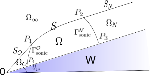
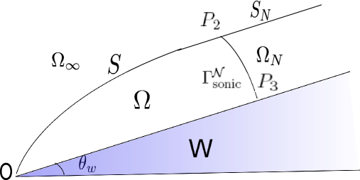
We consider this problem in the self-similar coordinates. Using the symmetry with respect to the $\xi_{1}$–axis, the problem can be posed in the region:

$$\Lambda=\mathbb{R}^{2}_{+}\setminus\{\bm{\xi}\;:\;\xi_{2}>\max(0,\xi_{1}\tan\theta_{\rm w})\}.$$

Denote by $\varphi_{\infty}$ the pseudo-potential of the incoming state.

Definition 7.9.

$\varphi\in C^{0,1}(\overline{\Lambda})$ is a weak solution of the Prandtl-Meyer reflection problem if $\varphi$ satisfies equation (2.5) in $\Lambda$, the boundary conditions (7.3) on $\partial\Lambda$, and the asymptotic conditions:

$$\lim_{R\to\infty}\|\varphi-\varphi_{\infty}\|_{C(L_{\theta}\setminus B_{R}(\mathbf{0}))}=0$$

along ray $L_{\theta}:=\{\xi_{1}=\xi_{2}\cot\theta,\xi_{2}>0\}$ for each $\theta\in(\theta_{\rm w},\pi)$ in the weak sense (as in Definition 7.1).

We consider the solutions with the structure shown in Figs. 7.6–7.6. These solutions are piecewise-smooth and equal to the constant states outside region $\Omega$ described below.

The constant states are defined as follows (see (Bae-Chen-Feldman-2, , §2) for the details and proofs): Given the constant self-similar state with velocity $\mathbf{v}_{\infty}=(u_{\infty},0)$ and density $\rho_{\infty}$ which is supersonic at the origin (the wedge vertex), there exist the detachment wedge angle $\theta_{\rm w}^{\rm d}\in(0,\frac{\pi}{2})$ and the sonic wedge angle $\theta_{\rm w}^{\rm s}\in(0,\theta_{\rm w}^{\rm d})$, which depend only on $(\rho_{\infty},u_{\infty})$, such that, for any wedge angle $\theta_{\rm w}\in(0,\theta_{\rm w}^{\rm d})$,

1. There exists a unique constant state $\varphi_{\mathcal{N}}$, which determines the normal reflection state of $\varphi_{\infty}$ from the wedge boundary $\partial W:=\{\xi_{1}>0,\xi_{2}=\xi_{1}\tan\theta_{\rm w}\}$; that is, $\varphi_{\mathcal{N}}$ satisfies that $\partial_{\bm{\nu}}\varphi_{\mathcal{N}}=0$ on $\partial W$, half-line $S_{\mathcal{N}}:=\{\bm{\xi}\;:\;\varphi_{\mathcal{N}}=\varphi_{\infty}\}\cap\{\xi_{2}>0\}$ lies in $\Lambda$ and is parallel to $\partial W$, and the Rankine-Hugoniot condition holds on $S_{\mathcal{N}}$:

   $$\rho_{\infty}\partial_{\bm{\nu}}\varphi_{\infty}=\rho_{\mathcal{N}}\partial_{\bm{\nu}}\varphi_{\mathcal{N}}\qquad\,\,\mbox{on $S_{\mathcal{N}}$}.$$

2. There exists a constant state $\varphi_{\mathcal{O}}$ such that $\partial_{\bm{\nu}}\varphi_{\mathcal{O}}=0$ on $\partial W$, half-line $S_{\mathcal{O}}:=\{\bm{\xi}\;:\;\varphi_{\mathcal{O}}=\varphi_{\infty}\}\cap\{\xi_{2}>0\}$ lies in $\Lambda$, the wedge vertex is on $\overline{S_{\mathcal{O}}}$ (i.e., $\mathbf{0}\in\overline{S_{\mathcal{O}}}$), and the Rankine-Hugoniot condition holds on $S_{\mathcal{O}}$:

   $$\rho_{\infty}\partial_{\bm{\nu}}\varphi_{\infty}=\rho_{\mathcal{O}}\partial_{\bm{\nu}}\varphi_{\mathcal{O}}\qquad\,\,\mbox{on $S_{\mathcal{O}}$}.$$

   In fact, there exist two states for $\varphi_{\mathcal{O}}$, weak and strong, and we always choose the weak one with the smaller density (so that the unique state $\varphi_{\mathcal{O}}$ is often referred).

3. $\varphi_{\mathcal{O}}$ is supersonic (resp. subsonic) at the origin for all $\theta_{\rm w}\in(0,\theta_{\rm w}^{\rm s})$ (resp. $\theta_{\rm w}\in(\theta_{\rm w}^{\rm s},\theta_{\rm w}^{\rm d}))$. This determines the supersonic and subsonic Prandtl-Meyer reflection configurations below.

Next, we define the points, lines, and regions in Figs. 7.6–7.6 for a given wedge angle $\theta_{\rm w}\in(0,\theta_{\rm w}^{\rm d})$ as follows:

1. The sonic arcs $\Gamma_{\text{\rm sonic}}^{\mathcal{N}}$ and $\Gamma_{\text{\rm sonic}}^{\mathcal{O}}$ are the arcs (defined below) of the sonic circles of the constant states $\varphi_{\mathcal{N}}$ and $\varphi_{\mathcal{O}}$, respectively, with the centers on $\partial W$, since these states satisfy the slip boundary condition on $\partial W$:

   • $\Gamma_{\text{\rm sonic}}^{\mathcal{N}}$ is the upper arc of $\partial B_{c_{\mathcal{N}}}(O_{\mathcal{N}})$ between lines $\partial W$ and $S_{\mathcal{N}}$. It follows that $\Gamma_{\text{\rm sonic}}^{\mathcal{N}}\subset\Lambda$, since $\partial B_{c_{\mathcal{N}}}(O_{\mathcal{N}})$ intersects the full line $S_{\mathcal{N}}$ at two points. Denote the endpoints of $\Gamma_{\text{\rm sonic}}^{\mathcal{N}}$ by $P_{2}$ and $P_{3}$, which lie on $S_{\mathcal{N}}$ and $\partial W$, respectively.

   • Arc $\Gamma_{\text{\rm sonic}}^{\mathcal{O}}$ is defined only for the supersonic reflection configurations, i.e., for $\theta_{\rm w}\in(0,\theta_{\rm w}^{\rm s})$. In this case, $\partial B_{c_{\mathcal{O}}}(O_{\mathcal{O}})$ intersects half-line $S_{\mathcal{O}}$ at two points within $\Lambda$, and $\Gamma_{\text{\rm sonic}}^{\mathcal{O}}$ is the lower arc of $\partial B_{c_{\mathcal{O}}}(O_{\mathcal{O}})$ between lines $\partial W$ and $S_{\mathcal{O}}$. Then $\Gamma_{\text{\rm sonic}}^{\mathcal{O}}\subset\Lambda$. Denote the endpoints of $\Gamma_{\text{\rm sonic}}^{\mathcal{O}}$ by $P_{1}$ and $P_{4}$, which lie on $S_{\mathcal{O}}$ and $\partial W$, respectively.

   • For the supersonic configurations, $S_{{\mathcal{O}},{\rm seg}}$ is segment $OP_{1}$. Note that $S_{{\mathcal{O}},{\rm seg}}\subset S_{\mathcal{O}}$.

   • $S_{{\mathcal{N}},{\rm seg}}$ is the portion of $S_{\mathcal{N}}$ with the left endpoint $P_{2}$, i.e., $S_{{\mathcal{N}},{\rm seg}}=S_{\mathcal{N}}\cap\{\xi_{1}>\xi_{1,P_{2}}\}$.

2. $\Gamma_{\text{\rm wedge}}$ is the segment of $\partial W$ between points $P_{3}$ and $P_{4}$ for the supersonic case (resp. between $\bm{0}$ and $P_{3}$ for the subsonic case).

3. There exists a smooth shock curve $\Gamma_{\text{\rm shock}}$ with the following properties:

   • For the supersonic reflection configurations, $\Gamma_{\text{\rm shock}}$ has endpoints $P_{1}$ and $P_{2}$;

   • For the subsonic reflection configurations, $\Gamma_{\text{\rm shock}}$ has endpoints $P_{2}$ and $O$;

   • $\Gamma_{\text{\rm shock}}$, $\Gamma_{\text{\rm sonic}}^{\mathcal{N}}$, $\Gamma_{\text{\rm wedge}}$, and $\Gamma_{\text{\rm sonic}}^{\mathcal{O}}$ do not have common points except at their end points.

4. $\Omega$ is the domain bounded by the curve formed by $\overline{\Gamma_{\text{\rm shock}}}$, $\overline{\Gamma_{\text{\rm sonic}}^{\mathcal{N}}}$, $\overline{\Gamma_{\text{\rm wedge}}}$, and $\overline{\Gamma_{\text{\rm sonic}}^{\mathcal{O}}}$.

5. For the supersonic reflection configurations, $\Omega_{\mathcal{O}}$ is the region bounded by arc $\overline{\Gamma_{\text{\rm sonic}}^{\mathcal{O}}}$ and the straight segments $\overline{OP_{1}}$ and $\overline{OP_{4}}$.

6. $\Omega_{\mathcal{N}}$ is the unbounded region with the boundary consisting of arc $\overline{\Gamma_{\text{\rm sonic}}^{\mathcal{N}}}$, and the straight half-lines $\partial W\cap\{\xi_{1}\geq\xi_{1P_{3}}\}$ and $S_{\mathcal{N}}\cap\{\xi_{1}\geq\xi_{1P_{2}}\}$.

7. $\Omega_{\infty}:=\Lambda\setminus\overline{\Omega_{\mathcal{O}}\cup\Omega\cup\Omega_{\mathcal{N}}}$ for the supersonic case, and $\Omega_{\infty}:=\Lambda\setminus\overline{\Omega\cup\Omega_{\mathcal{N}}}$ for the subsonic case.

Now we define a class of solutions of the Prandtl-Meyer reflection problem with the structure as in Figs. 7.6–7.6.

Definition 7.10.

Let $(\rho_{\infty},(u_{\infty},0))$ be a supersonic state in $\Omega_{\infty}$, and let $\theta_{\rm w}^{\rm d}$ and $\theta_{\rm w}^{\rm s}$ be the corresponding detachment and sonic angles. Let $\theta_{\rm w}\in(\theta_{\rm w}^{\rm d},\frac{\pi}{2})$. A function $\varphi\in C^{0,1}(\overline{\Lambda})$ is an admissible solution of the Prandtl-Meyer reflection problem if $\varphi$ is a solution in the sense of Definition 7.9 and satisfies the following properties:

1. The structure of solution is the following:

   • If $\theta_{\rm w}\in(0,\theta_{\rm w}^{\rm s})$, then the solution is of supersonic reflection configuration as in Fig. 7.6 and satisfies

     $$\varphi\in C^{1}(\overline{\Lambda}\setminus\overline{S_{{\mathcal{O}},{\rm seg}}\cup\Gamma_{\text{\rm shock}}\cup S_{{\mathcal{N}},{\rm seg}}}),$$ (7.28)

     $$\varphi\in C^{3}(\Omega)\cap C^{2}(\overline{\Omega}\setminus\overline{\Gamma_{\text{\rm sonic}}^{\mathcal{O}}\cup\Gamma_{\text{\rm sonic}}^{\mathcal{N}}})\cap C^{1}(\overline{\Omega}),$$ (7.29)

     $$\varphi=\begin{cases}\,\varphi_{\infty}\qquad&\mbox{in $\Omega_{\infty}$},\\[0.85358pt] \,\varphi_{\mathcal{O}}&\mbox{in $\Omega_{\mathcal{O}}$},\\[0.85358pt] \,\varphi_{\mathcal{N}}&\mbox{in $\Omega_{\mathcal{N}}$}{\rm;}\end{cases}$$ (7.30)

   • If $\theta_{\rm w}\in[\theta_{\rm w}^{\rm s},\theta_{\rm w}^{\rm d})$, then the solution is of subsonic reflection configuration as in Fig. 7.6 and satisfies

     $$\varphi\in C^{1}(\overline{\Lambda}\setminus\overline{\Gamma_{\text{\rm shock}}\cup S_{{\mathcal{N}},{\rm seg}}}),$$ (7.31)

     $$\varphi\in C^{3}(\Omega)\cap C^{2}(\overline{\Omega}\setminus(\{O\}\cup\overline{\Gamma_{\text{\rm sonic}}^{\mathcal{N}}}))\cap C^{1}(\overline{\Omega}),$$ (7.32)

     $$\varphi=\begin{cases}\,\varphi_{\infty}\qquad&\mbox{in $\Omega_{\infty}$},\\[0.85358pt] \,\varphi_{\mathcal{O}}(O)&\mbox{at $O$},\\[0.85358pt] \,\varphi_{\mathcal{N}}&\mbox{in $\Omega_{\mathcal{N}}$}{\rm,}\end{cases}$$ (7.33)

     $$D\varphi(O)=D\varphi_{\mathcal{O}}(O).$$ (7.34)

2. The shock curve $\Gamma_{\text{\rm shock}}$ is $C^{2}$ in its relative interior.

3. Equation (2.5) is strictly elliptic in $\overline{\Omega}\backslash(\overline{\Gamma_{\text{\rm sonic}}^{\mathcal{N}}}\cup\overline{\Gamma_{\text{\rm sonic}}^{\mathcal{O}}})$ for the supersonic case and in $\overline{\Omega}\backslash(\overline{\Gamma_{\text{\rm sonic}}^{\mathcal{N}}}\cup\{O\})$ for the subsonic case.

4. $\partial_{\bm{\nu}}\varphi_{\infty}>\partial_{\bm{\nu}}\varphi>0$ on $\Gamma_{\text{\rm shock}}$, where $\bm{\nu}$ is the normal vector to $\Gamma_{\text{\rm shock}}$ pointing into $\Omega$.

5. $\partial_{\mathbf{e}_{S_{\mathcal{O}}}}(\varphi_{\infty}-\varphi)\leq 0$ and $\partial_{\mathbf{e}_{S_{\mathcal{N}}}}(\varphi_{\infty}-\varphi)\leq 0$ in $\Omega$, where vectors $\mathbf{e}_{S_{\mathcal{O}}}$ and $\mathbf{e}_{S_{\mathcal{N}}}$ are parallel to lines $S_{\mathcal{O}}$ and $S_{\mathcal{N}}$, respectively, oriented towards the interior of $\Gamma_{\text{\rm shock}}$ from points $P_{1}$ and $P_{2}$, respectively;

Remark 7.11.

A version of Remark 7.3 holds in the present case, with the only difference that the potential function of the incoming state is $\varphi_{\infty}$ here, instead of $\varphi_{1}$.

Remark 7.12.

$\varphi$ in $\Omega$ is not a constant state. Indeed, if $\varphi$ is a constant state in $\Omega$, then $\varphi=\varphi_{\mathcal{N}}$ in $\Omega$, which follows from (7.30) and (7.33) in the supersonic and subsonic cases, respectively. On the other hand, we obtain that $\varphi=\varphi_{\mathcal{O}}$ in $\Omega$, which follows from both (7.30) for the supersonic case (since $\varphi$ is $C^{1}$ across $\Gamma_{\text{\rm sonic}}^{\mathcal{O}}$) and the property that $(\varphi,D\varphi)=(\varphi_{2},D\varphi_{2})$ at $O$ for the subsonic case. However, $\varphi_{\mathcal{O}}$ and $\varphi_{\mathcal{N}}$ are two different states, which can be seen from their definitions, since line $S_{\mathcal{N}}$ is parallel to $\partial W$ (so that these lines do not coincide), while $S_{\mathcal{O}}$ intersects $\partial W$ at point $O$.

Lemma 7.13.

Definition 7.10 is equivalent to the definition of admissible solutions in Bae-Chen-Feldman-2 ; see Definition 2.14 there.

The proof of Lemma 7.13 follows closely the proof of Lemma 7.6 with mostly notational changes, so we skip this proof here.

From Lemma 7.13, the results of baechenfeldman-prandtlmayerReflection ; Bae-Chen-Feldman-2 for the existence and properties of admissible solutions apply to the solutions in the sense of Definition 7.2. We list some of these properties in the following theorem.

Theorem 7.5.

Let $(\rho_{\infty},(u_{\infty},0))$ be a supersonic state in $\Omega_{\infty}$, and let $\theta_{\rm w}^{\rm d}$ and $\theta_{\rm w}^{\rm s}$ be the corresponding detachment and sonic angles. Then any admissible solution of the Prandtl-Meyer reflection problem with wedge angle $\theta_{\rm w}\in(0,\theta_{\rm w}^{\rm d})$ has the following properties:

1. Additional regularity:

   • If $\theta_{\rm w}\in(0,\theta_{\rm w}^{\rm s})$, i.e., when the solution is of supersonic reflection configuration as in Fig. 7.6, then $\varphi\in C^{1,1}(\overline{\Omega_{\mathcal{O}}\cup\Omega\cup\Omega_{\mathcal{N}}})$ and $\varphi\in C^{\infty}(\overline{\Omega}\setminus\overline{\Gamma_{\text{\rm sonic}}^{\mathcal{O}}\cup\Gamma_{\text{\rm sonic}}^{\mathcal{N}}})$;

   • If $\theta_{\rm w}\in[\theta_{\rm w}^{\rm s},\theta_{\rm w}^{\rm d})$, i.e., when the solution is of subsonic reflection configuration as in Fig. 7.6, then $\varphi\in C^{1,\alpha}(\overline{\Omega\cup\Omega_{\mathcal{N}}})\cap C^{1,1}(\overline{\Omega\cup\Omega_{\mathcal{N}}}\setminus\{O\})$ and $\varphi\in C^{\infty}(\overline{\Omega}\setminus(\{O\}\cup\overline{\Gamma_{\text{\rm sonic}}^{\mathcal{N}}}))$ for some $\alpha\in(0,1)$, depending on $(\rho_{\infty},u_{\infty},\theta_{\rm w})$ and non-increasing with respect to $\theta_{\rm w}$.

2. The shock curve $\Gamma_{\text{\rm shock}}$ is $C^{\infty}$ in its relative interior.

3. $\Gamma_{\text{\rm shock}}$ has the following regularity up to the endpoints: In the supersonic case, the whole shock curve $\overline{S_{{\mathcal{O}},{\rm seg}}\cup\Gamma_{\text{\rm shock}}\cup S_{{\mathcal{N}},{\rm seg}}}$ is $C^{2,\beta}$ for any $\beta\in(0,1)$. In the subsonic case, curve $\overline{\Gamma_{\text{\rm shock}}\cup S_{{\mathcal{N}},{\rm seg}}}$ is $C^{1,\alpha}$ with $\alpha$ as in (i).

4. For each $\mathbf{e}\in Con(\mathbf{e}_{S_{\mathcal{O}}},\mathbf{e}_{S_{\mathcal{N}}})$,

   $$\partial_{\mathbf{e}}(\varphi_{\infty}-\varphi)<0\qquad\,\,\mbox{in $\overline{\Omega}$},$$ (7.35)

   where vectors $\mathbf{e}_{S_{\mathcal{O}}}$ and $\mathbf{e}_{S_{\mathcal{N}}}$ are introduced in Definition 7.10(v), and notation (7.26) has been used.

5. Denote by $\bm{\nu}_{\rm w}$ the interior unit normal vector to $\Gamma_{\text{\rm wedge}}$ pointing into $\Omega$, i.e., $\bm{\nu}_{\rm w}=(-\sin\theta_{\rm w},\cos\theta_{\rm w})$. Then

   $$\partial_{\bm{\nu}_{\rm w}}(\varphi-\varphi_{\mathcal{O}})\leq 0,\quad\partial_{\bm{\nu}_{\rm w}}(\varphi-\varphi_{\mathcal{N}})\leq 0\qquad\mbox{in $\overline{\Omega}$}.$$

Proof.

Properties (i)–(iii) are from (Bae-Chen-Feldman-2, , Theorem 2.16). Properties (iv) and (v) are shown in (Bae-Chen-Feldman-2, , Lemmas 3.2 and 3.6), where the results are stated in a rotated coordinate system, in which the $\xi_{2}$–variable is in the direction of $\bm{\nu}_{\rm w}$. ∎

Theorem 7.6.

Let $(\rho_{\infty},(u_{\infty},0))$ be a supersonic state in $\Omega_{\infty}$, and let $\theta_{\rm w}^{\rm d}$ be the corresponding detachment angle. Then, for any $\theta_{\rm w}\in(0,\theta_{\rm w}^{\rm d})$, there exists an admissible solution of the Prandtl-Meyer reflection problem.

The existence of solutions follows from (Bae-Chen-Feldman-2, , Theorem 2.15).

Now, similar to Lemma 7.8, we have

Lemma 7.14.

The following statements hold:

1. Any admissible solution in the sense of Definition 7.10 satisfies the conditions of Theorems 2.1 and 2.3.

2. Any global weak solution of the Prandtl-Meyer reflection problem in the sense of Definition 7.9 with properties (i)–(iv) of Definition 7.10 and with shock $\Gamma_{\text{\rm shock}}$ being a strictly convex graph in the sense of (2.18)–(2.19) satisfies property (v) of Definition 7.10.

Proof.

We first discuss the proof of assertion (i).

Conditions (A1)–(A5) follow directly as in Lemma 7.8. In particular, in (A5), $Con=Con(\mathbf{e}_{S_{\mathcal{O}}},\mathbf{e}_{S_{\mathcal{N}}})$, where we have used (7.26). Also, $A=P_{1}$ and $B=P_{2}$, where $P_{1}:=O$ in the subsonic/sonic case.

For condition (A6), we choose $\mathbf{e}=\bm{\nu}_{\rm w}$, where $\bm{\nu}_{\rm w}$ is defined in Theorem 7.5(v). Then $\mathbf{e}\in Con$, which can be seen from the fact that $u_{\mathcal{O}}>0$ and $v_{\mathcal{O}}>0$ with $\frac{v_{\mathcal{O}}}{u_{\mathcal{O}}}>\tan\theta_{\rm w}$, and $\mathbf{e}_{{\mathcal{N}}}=-(\cos\theta_{\rm w},\sin\theta_{\rm w})$.

In the argument below, the local extrema are relative to $\overline{\Omega}$. Also, we discuss the supersonic and subsonic/sonic cases together and define $\overline{\Gamma_{\text{\rm sonic}}^{\mathcal{O}}}:=\{O\}$ and $P_{1}:=O$ for the subsonic/sonic case.

Recall the boundary conditions:

$$\partial_{\bm{\nu}}\varphi=0,\quad\partial_{\bm{\nu}}\varphi_{\mathcal{O}}=0,\quad\partial_{\bm{\nu}}\varphi_{\mathcal{N}}=0\qquad\;\;\mbox{on $\overline{\Gamma}_{\text{\rm wedge}}$}.$$

Also, $D\varphi=D\varphi_{\mathcal{O}}$ on $\overline{\Gamma_{\text{\rm sonic}}^{\mathcal{O}}}$ by Definition 7.10(i). Thus, $\partial_{\mathbf{e}}(\varphi-\varphi_{\mathcal{O}})=0$ on $\overline{\Gamma}_{\text{\rm wedge}}\cup\overline{\Gamma_{\text{\rm sonic}}^{\mathcal{O}}}$, which is the global maximum over $\overline{\Omega}$ by Theorem 7.5(v). Since $\varphi$ is not a constant state, arguing as in Step 5 of the proof of Lemma 7.8, we find that, if $\phi_{\mathbf{e}}$ attains its local minimum on $\overline{\Gamma}_{\text{\rm wedge}}\cup\overline{\Gamma_{\text{\rm sonic}}^{\mathcal{O}}}$, then $\phi_{\mathbf{e}}$ is constant in $\Omega$. Similarly, using that $D\varphi=D\varphi_{\mathcal{N}}$ on $\overline{\Gamma_{\text{\rm sonic}}^{\mathcal{N}}}$ and arguing as above, we conclude that $\phi_{\mathbf{e}}$ cannot attain its local minimum on $\overline{\Gamma_{\text{\rm sonic}}^{\mathcal{N}}}$, unless $\phi_{\mathbf{e}}$ is constant in $\Omega$. Combining all the facts together, we conclude that, if $\phi_{\mathbf{e}}$ attains its local minimum on $\overline{\Gamma_{\text{\rm sonic}}^{\mathcal{N}}}\cup\overline{\Gamma}_{\text{\rm wedge}}\cup\overline{\Gamma_{\text{\rm sonic}}^{\mathcal{O}}}$, then $\phi_{\mathbf{e}}$ is constant in $\Omega$.

We now show that, if $\phi_{\mathbf{e}}$ is constant in $\Omega$, then $\varphi$ is a constant state in $\Omega$. To fix notations, we consider first the supersonic case. Since conditions (A1)–(A5) have been verified, we can apply Lemma 3.2. We work in the $(S,T)$–coordinates with basis $\{\mathbf{e},\mathbf{e}^{\perp}\}$ and origin $O$, where the orientation of $\mathbf{e}^{\perp}$ is as in Lemma 3.2. Then $T_{P_{4}}<T_{P_{1}}<T_{P_{2}}<T_{P_{3}}$, where we have used that $A=P_{1}$ and $B=P_{2}$. Also,

$$\Gamma_{\text{\rm sonic}}^{\mathcal{O}}=\{S=f_{{\mathcal{O}}}(T),\;T\in(T_{P_{4}},\,T_{P_{1}})\},\,\,\Gamma_{\text{\rm sonic}}^{\mathcal{N}}=\{S=f_{{\mathcal{N}}}(T),\;T\in(T_{P_{2}},\,T_{P_{3}})\},$$

where $f_{{\mathcal{O}}}\in C^{\infty}((T_{P_{4}},\,T_{P_{1}}))$ and $f_{{\mathcal{N}}}\in C^{\infty}((T_{P_{2}},\,T_{P_{3}}))$ are positive. With this, we obtain

$$\Omega=\{(S,T)\,:\,T\in(T_{P_{4}},\,T_{P_{3}}),\;\;S\in(0,\,\hat{f}(T))\},$$

where $\hat{f}\in C(T_{P_{4}},\,T_{P_{3}})$ satisfies

$$\hat{f}=f_{{\mathcal{O}}}\;\mbox{on $(T_{P_{4}},\,T_{P_{1}})$},\,\,\hat{f}=f_{\mathbf{e}}\;\mbox{on $(T_{P_{1}},\,T_{P_{2}})$},\,\,\hat{f}=f_{{\mathcal{N}}}\;\mbox{on $(T_{P_{2}},\,T_{P_{3}})$}.$$ (7.36)

Let $\phi_{\mathbf{e}}\equiv a$ in $\Omega$. Then, from the structure of $\Omega$ described above, $\phi(S,T)=aS+g(T)$ in $\Omega$ for some $g\in C^{1}(\mathbb{R})$. Then, noting that $D\varphi=D\varphi_{{\mathcal{N}}}$ on $\Gamma_{\text{\rm sonic}}^{{\mathcal{N}}}$, we obtain

$$g^{\prime}(T)=\partial_{\mathbf{e}^{\perp}}\phi(f_{{\mathcal{N}}}(T),T)=D(\varphi_{{\mathcal{N}}}-\varphi_{\infty})\cdot\mathbf{e}^{\perp}\qquad\mbox{for all $T\in(T_{P_{2}},\,T_{P_{3}})$},$$

where we have used that $D(\varphi_{{\mathcal{N}}}-\varphi_{\infty})$ is a constant vector. Thus, $g^{\prime}(T)$ is constant on $(T_{P_{2}},\,T_{P_{3}})$ so that $\phi(S,T)=aS+bT+c$ in $\hat{\Omega}:=\{(S,T)\,:\,T\in(T_{P_{2}},\,T_{P_{3}}),\;S\in(0,\,f_{{\mathcal{N}}}(T))\}\subset\Omega$. Then, arguing as in Step 5 of the proof of Lemma 7.8, we conclude that $\varphi$ is a constant state in $\Omega$, which is a contradiction. For the subsonic/sonic case, the argument is the same, except the structure of $\Omega$, where now $P_{4}=P_{1}=O$, and $f_{{\mathcal{O}}}$ is not present in (7.36).

Therefore, Case (iii) of (A6) holds with $\mathbf{e}=\bm{\nu}_{\rm w}$, $\Gamma_{1}:=\Gamma_{\text{\rm sonic}}^{\mathcal{N}}\cup\overline{\Gamma}_{\text{\rm wedge}}\cup\Gamma_{\text{\rm sonic}}^{\mathcal{O}}$ for the supersonic case (resp. $\Gamma_{1}:=\Gamma_{\text{\rm sonic}}^{\mathcal{N}}\cup\overline{\Gamma}_{\text{\rm wedge}}\setminus\{P_{2}\}$ for the subsonic case), and $\Gamma_{2}=\emptyset$.

We now show that conditions (A7)–(A10) are satisfied with $\hat{\Gamma}_{0}=\overline{\Gamma_{\text{\rm sonic}}^{\mathcal{N}}}\setminus\{P_{2}\}$, $\hat{\Gamma}_{1}=\Gamma_{\text{\rm wedge}}^{0}$, $\hat{\Gamma}_{2}=\emptyset$, and $\hat{\Gamma}_{3}=\overline{\Gamma_{\text{\rm sonic}}^{\mathcal{O}}}\setminus\{P_{1}\}$ for the supersonic case (resp. $\hat{\Gamma}_{3}=\emptyset$ for the subsonic case). Indeed, then (A7) clearly holds. Also, (A8) holds since $D\varphi=D\varphi_{\mathcal{N}}$ on $\overline{\Gamma_{\text{\rm sonic}}^{\mathcal{N}}}$, and $D\varphi=D\varphi_{\mathcal{O}}$ on $\overline{\Gamma_{\text{\rm sonic}}^{\mathcal{O}}}$ for the supersonic case.

Condition (A9) on $\hat{\Gamma}_{1}=\Gamma_{\text{\rm wedge}}^{0}$ can be checked as follows: If $\mathbf{e}\cdot\bm{\tau}\neq 0$ on $\Gamma_{\text{\rm wedge}}^{0}$, then the argument of Step 5 in the proof of Lemma 7.8 applies here to yield that $\phi_{\mathbf{e}}$ cannot attain the local minima or maxima on $\Gamma_{\text{\rm wedge}}^{0}$. In the other case, when $\mathbf{e}=\pm\bm{\nu}_{\rm w}$, we use the boundary condition:

$$\partial_{\bm{\nu}}\varphi=0\qquad\mbox{on $\Gamma_{\text{\rm wedge}}^{0}$}$$

to derive that $\partial_{\bm{\nu}}\phi=-u_{\infty}\sin\theta_{\rm w}$ on $\Gamma_{\text{\rm wedge}}$, similar to (7.19). Also, on $\hat{\Gamma}_{0}=\overline{\Gamma_{\text{\rm sonic}}^{\mathcal{N}}}\setminus\{P_{2}\}$, $D\varphi=D\varphi_{\mathcal{N}}$ so that $\phi_{\mathbf{e}}=\partial_{\mathbf{e}}(\varphi_{\mathcal{N}}-\varphi_{\infty})=const$. The argument on $\hat{\Gamma}_{3}=\overline{\Gamma_{\text{\rm sonic}}^{\mathcal{O}}}\setminus\{P_{1}\}$ in the supersonic case is similar. This verifies (A9). Case (i) of (A10) clearly holds here.

To prove assertion (ii), we follow directly the argument of Step 7 in the proof of Lemma 7.8 with mostly notational changes, e.g., now $\varphi_{\infty}$ replaces $\varphi_{1}$. ∎

Therefore, we have

Theorem 7.7.

If $\varphi$ is an admissible solution of the Prandtl-Meyer reflection problem, then its shock curve $\Gamma_{\text{\rm shock}}$ is uniformly convex in the sense described in Theorem 2.3. Moreover, for a weak solution of the Prandtl-Meyer reflection problem in the sense of Definition 7.9 with properties (i)–(iv) of Definition 7.10, the transonic shock $\Gamma_{\text{\rm shock}}$ is a strictly convex graph as in (2.18)–(2.19) if and only if property (v) of Definition 7.10 holds.

Appendix A  Paths Connecting Endpoints of the Minimal and Maximal Chains

For $\Lambda\subset\mathbb{R}^{n}$, we denote

$$\Lambda_{r}:=\{\bm{\xi}\in\Lambda\;:\;{\rm dist}(\bm{\xi},\partial\Lambda)>r\}.$$ (A.1)

Lemma A.1.

Let $\Lambda\subset\mathbb{R}^{n}$ be an open set such that $\Lambda_{r}$ is connected for each $r\in[0,r_{0}]$ with given $r_{0}>0$. Let $P,Q\in\overline{\Lambda}$ be such that $B_{r}(P)\cap\Lambda_{\rho}$ and $B_{r}(Q)\cap\Lambda_{\rho}$ are connected for each $0\leq\rho<r\leq r_{0}$. Then there exists a continuous curve ${\mathcal{S}}$ with endpoints $P$ and $Q$ such that ${\mathcal{S}}^{0}\subset\Lambda$. More precisely, ${\mathcal{S}}=g([0,1])$, where $g\in C([0,1];\mathbb{R}^{n})$, $g$ is locally Lipschitz on $(0,1)$, $g(0)=P$, $g(1)=Q$, and $g(t)\in\Lambda$ for all $t\in(0,1)$.

Proof.

We first note that, after points $P$ and $Q$ are fixed, we can assume that $\Lambda$ is a bounded set; otherwise, we replace $\Lambda$ by $\Lambda\cap B$, where $B$ is an open ball and $P,Q\in B$.

We divide the proof into three steps.

1. We notice that, if $P,Q\in\Lambda_{r}$ for some $r\in[0,r_{0})$, then there exists a piecewise-linear path ${\mathcal{S}}$ with a finite number of corner points connecting $P$ to $Q$ such that ${\mathcal{S}}\subset\Lambda_{r/2}$. This is obtained via covering $\overline{\Lambda_{r}}$ by balls $B_{r/2}(\xi_{i})$, $i=1,\dots,N$, with each $\xi_{i}\in\overline{\Lambda}_{r}$ and via noting that, since $\Lambda_{r}$ is connected, then any $\xi_{i}$ and $\xi_{j}$ can be connected by a piecewise-linear path with at most $N$ corners, each section of which is a straight segment connecting centers of two intersecting balls of the cover.

Thus, the path connecting $\xi_{i}$ to $\xi_{j}$ lies in $\cup_{k=1}^{N}B_{r/2}(\xi_{k})\subset\Lambda_{r/2}$. Then we connect $P$ to $Q$ by first connecting $P$ (resp. $Q$) to the nearest center of ball $\xi_{i}$ (resp. $\xi_{j}$) via a straight segment that lies in $B_{r_{2}}(\xi_{i})$ (resp. $B_{r_{2}}(\xi_{j})$), and next connect $\xi_{i}$ to $\xi_{j}$ as above. In this way, the whole path ${\mathcal{S}}$ between $P$ and $Q$ is Lipschitz up to the endpoints and lies in $\Lambda_{r/2}$. Clearly, there exists $g\in C^{0,1}([0,1];\mathbb{R}^{n})$ with $g(0)=P$, $g(1)=Q$, and $g(t)\in\Lambda_{r/2}$ for all $t\in[0,1]$ such that ${\mathcal{S}}=g([0,1]$. Therefore, this lemma is proved for any $P,Q\in\Lambda$.

2. Now we consider the case when $P\in\partial\Lambda$ and $Q\in\Lambda$. Since $\Lambda$ is open, there exists a sequence $P_{m}\to P$ with $P_{m}\in\Lambda$ for $m=1,2,\dots$. Then $P_{m}\in\Lambda_{r_{m}}$ with $r_{m}>0$ and $r_{m}\to 0$. Thus, taking a subsequence, we can assume without loss of generality that $0<r_{m}<\frac{r_{0}}{m}$ for all $m$.

As proved in Step 1, $P_{1}$ can be connected to $Q$ by a Lipschitz curve that is parameterized by $g\in C^{0,1}([\frac{1}{2},1];\mathbb{R}^{n})$ with

$$g(\frac{1}{2})=P_{1},\,\,\,\,g(1)=Q,\quad\,\,\,g(t)\in\Lambda_{\tilde{r}}\,\,\mbox{for all $t\in[0,1]$},$$

where $\tilde{r}>0$. Since $(B_{r}(P)\cap\Lambda)_{\varepsilon}=B_{r-\varepsilon}(P)\cap\Lambda_{\varepsilon}$ for all $\varepsilon\in[0,\frac{r}{2})$, then the assumptions of this lemma allow to apply the result of Step 1 to sets $B_{r_{0}/m}(P)\cap\Lambda$ for $m=1,2,\dots$. Thus, for each $m=1,2,\dots$, we obtain a Lipschitz path between $P_{m}$ and $P_{m+1}$ which lies in $B_{r_{0}/m}(P)\cap\Lambda$ and is parameterized by $\displaystyle g\in C^{0,1}([\frac{1}{m+2},\frac{1}{m+1}];\mathbb{R}^{n})$ with

$$\begin{split}&g(\frac{1}{m+1})=P_{m},\;\;\;\;g(\frac{1}{m+2})=P_{m+1},\\ &g(t)\in B_{\frac{r_{0}}{m}}(P)\cap\Lambda_{\tilde{r}_{m}}\,\,\,\,\mbox{ for all $t\in[\frac{1}{m+2},\frac{1}{m+1}]$}.\end{split}$$

Combining the above together, we obtain a function $g:(0,1]\to\mathbb{R}^{n}$ such that $\displaystyle g\in C([0,1];\mathbb{R}^{n})\cap C^{0,1}_{\rm loc}((0,1];\mathbb{R}^{n})$ with

$$\begin{split}\lim_{t\to 0+}g(t)=P,\quad g(1)=Q,\;\quad\;g(t)\in\Lambda\;\mbox{ for all $t\in(0,1]$}.\end{split}$$

This completes the proof for the case when $P\in\partial\Lambda$ and $Q\in\Lambda$.

3. The remaining case for both $P,Q\in\partial\Lambda$ now readily follows, by connecting each of $P$ and $Q$ to some $C\in\Lambda$ and taking the union of the paths. ∎

Lemma A.2.

Let $\Omega\subset\mathbb{R}^{2}$ satisfy the conditions stated at the beginning of §3.3, and let $r^{*}$ be the constant from Lemma 3.10. Let $\Omega_{\rho}$ be defined as in (A.1). Then there exists $r_{0}\in(0,\frac{r^{*}}{10}]$ such that sets $\Omega_{\rho}$ are connected for all $\rho\in[0,r_{0}]$, and sets $B_{r}(E)\cap\Omega_{\rho}$ are connected for any $E\in\overline{\Omega}$ and $0\leq\rho<r\leq r_{0}$. Moreover, if $0\leq\rho<r\leq 2r_{0}$, $P\in\overline{\Omega}$, and ${\rm dist}(P,\partial\Omega)<r$, then

$${\rm dist}(E,\partial\Omega\cap B_{r}(P))\leq C\rho\qquad\;\mbox{ for each $E\in\partial\Omega_{\rho}\cap B_{r}(P)$},$$ (A.2)

where $C$ depends only on the constants in the assumptions on $\Omega$.

Proof.

Throughout this proof, $C$ denotes a universal constant, depending only on $\Omega$. We divide the proof into two steps.

1. We first describe the structure of $\partial\Omega_{\rho}$ for sufficiently small $\rho>0$ and show that $\Omega_{\rho}$ is connected for such $\rho$ and (A.2) holds.

Denote by $\Gamma_{i}$, $i=1,\dots,m$, the smooth regions of $\partial\Omega$ up to the corner points. Then, for $P\in\Omega$, we have

$${{\rm dist}}(P,\partial\Omega)=\min_{i=1,\dots,m}{{\rm dist}}(P,\Gamma_{i}).$$

Denote

$$\Omega_{i}=\{P\in\Omega\;:\;{\rm dist}(P,\partial\Omega)={\rm dist}(P,\Gamma_{i})\}.$$

Using that each $\Gamma_{i}$ is $C^{1,\alpha}$ up to the corner points, and the angles at the corner points are between $(0,\pi)$, we now show that there exists $r_{0}>0$ such that, for any $\rho\in(0,r_{0})$ and $i=1,\dots,m$, the set:

$$\Gamma_{i}^{\rho}:=\{P\in\Omega_{i}\;:\;{\rm dist}(P,\partial\Omega)=\rho\}$$

is a Lipschitz curve. In addition, $\Gamma_{i}^{\rho}$ is close to $\Gamma_{i}$ in the Lipschitz norm in the sense described bellow.

Consider first a curve $\Gamma=\{(s,t)\in\mathbb{R}^{2}\;:\;s=g(t)\}$ for some $g\in C^{1,\alpha}(\mathbb{R})$. Let $\rho>0$ and $\Gamma^{\rho}=\{(s,t)\in\mathbb{R}^{2}\;:\;s>g(t),\;{\rm dist}((s,t),\Gamma)=\rho\}$. Fix $t_{0}\in\mathbb{R}$ and $r>10\rho$, and denote $L:=\|g\|_{C^{0,1}([t_{0}-2r,t_{0}+2r])}$. Then we find that, for any $t_{1}\in[t_{0}-r,t_{0}+r]$, there exists $s_{1}\in[g(t_{1})+\rho,\;g(t_{1})+\rho\sqrt{L^{2}+1}]$ such that $(s_{1},t_{1})\in\Gamma^{\rho}$ and

$$\Gamma^{\rho}\cap\{(s,t)\in\mathbb{R}^{2}\;:\;|t-t_{0}|\leq r,\;s>s_{1}+L|t-t_{1}|\}=\emptyset$$

by noting that $B_{\rho}(s_{1},t_{1})\cap\Gamma=\emptyset$. From this,

$$\Gamma^{\rho}=\{(s,t)\in\mathbb{R}^{2}\;:\;s=g^{\rho}(t)\}$$

with $g^{\rho}\in C^{0,1}_{\rm loc}(\mathbb{R})$ and $\|g-g^{\rho}\|_{L^{\infty}([-r,r])}\leq\rho\sqrt{L^{2}+1}$. Moreover, fix $P\in\Gamma^{\rho}$. Then there exists $Q\in\Gamma$ such that ${\rm dist}(P,Q)=\rho$. It follows that

$$B_{\rho}(P)\cap\Gamma=\emptyset,\quad\;B_{\rho}(Q)\cap\Gamma^{\rho}=\emptyset.$$

From this, for any $r\in(0,1)$, we find that there exists $r_{0}\in(0,\frac{r}{10}]$ depending only on $r$, $\alpha$, and $\hat{L}:=\|g\|_{C^{1,\alpha}([3r,3r])}$ such that, if $\rho\in(0,r_{0}]$, then, for any $P=(g^{\rho}(t_{P}),t_{P})\in\Gamma^{\rho}\cap\{t\in[-r,r]\}$, we have

$$g^{\rho}(t) \geq g^{\rho}(t_{P})+g^{\prime}(t_{Q})(t-t_{P})-\hat{L}r^{\alpha}|t-t_{P}|$$

$$\geq g^{\rho}(t_{P})+g^{\prime}(t_{P})(t-t_{P})-\hat{L}(r^{\alpha}+\rho^{\alpha})|t-t_{P}|$$

for any $t\in[-2r,2r]$, where $Q:=(g(t_{Q}),t_{Q})$ a point such that ${\rm dist}(P,Q)=\rho$.

Then, noting that

$$|g(t)-g(t_{P})-g^{\prime}(t_{P})(t-t_{P})|\leq Lr^{\alpha}|t-t_{P}|\qquad\,\mbox{for any $t\in[-2r,2r]$},$$

and $\|g-g^{\rho}\|_{L^{\infty}([-r,r])}\leq\rho\sqrt{\hat{L}^{2}+1}$, we have

$$\|g-g^{\rho}\|_{C^{0,1}([-r,r])}\leq\hat{L}\rho^{\alpha}+\rho\sqrt{\hat{L}^{2}+1}.$$

Thus, for any $\varepsilon\in(0,1)$, reducing $r_{0}$, we obtain

$$\|g-g^{\rho}\|_{C^{0,1}([-r,r])}\leq\varepsilon\qquad\;\mbox{ if $\rho\leq r_{0}$}.$$ (A.3)

From this, under the conditions of Case (a) in the proof of Lemma 3.10, when (3.17) holds, we follow the argument in the proof of Lemma 3.10 and choosing sufficiently small $r_{0}$ and $\varepsilon$ in (A.3) to obtain that, for any positive $\rho<\min\{r,r_{0}\}$,

$$\begin{split}&\Omega_{\rho}\cap Q_{\frac{3r}{2}}=\{(s,t)\in Q_{\frac{3r}{2}}\;:\;s>g^{\rho}(t)\},\\ &\partial\Omega^{\rho}\cap Q_{\frac{3r}{2}}=\{(s,t)\in Q_{\frac{3r}{2}}\;:\;s=g^{\rho}(t)\}.\end{split}$$ (A.4)

Furthermore, under the conditions of Case (b) in the proof of Lemma 3.10, when (3.18)–(3.19) hold, we repeat the argument there by choosing small $r_{0}$ and $\varepsilon$, and conclude that, for any positive $\rho<\min\{r,r_{0}\}$,

$$\begin{split}&\Omega^{\rho}\cap Q_{3Nr}=\{(s,t)\in Q_{3Nr}\;:\;s>\max(g_{1}^{\rho}(t),g_{2}^{\rho}(t))\},\\[1.42262pt] &\partial\Omega^{\rho}\cap Q_{3Nr}=\{(s,t)\in Q_{3Nr}\;:\;s=\max(g_{1}^{\rho}(t),g_{2}^{\rho}(t))\},\end{split}$$ (A.5)

where $g_{1}^{\rho}$ and $g_{2}^{\rho}$ satisfy (A.3) with $g_{1}$ and $g_{2}$, respectively, and that there exists $t_{\rho}\in(-C\rho,C\rho)$ such that

$$\begin{split}&g_{1}^{\rho}(t)>g_{2}^{\rho}(t)\;\mbox{ for $t<t_{\rho}$},\qquad g_{1}^{\rho}(t)<g_{2}^{\rho}(t)\;\mbox{ for $t>t_{\rho}$}.\end{split}$$ (A.6)

We adjust $r_{0}$ so that $r_{0}\leq\frac{r^{*}}{10}$. Then, from (A.4)–(A.6) with $r=r^{*}$, we obtain that, for each $\rho\in(0,r_{0}]$, $\partial\Omega_{\rho}$ is a Lipschitz curve without self-intersection. It follows that $\Omega_{\rho}$ is simply-connected.

Also, combining (A.4) with (3.17) and (A.5)–(A.6) with (3.18)–(3.19) for $r=r_{0}$, choosing $\varepsilon$ small in (A.3) for $g,g_{1}$, and $g_{2}$, and adjusting $r_{0}$, we have

$${\rm dist}(\partial\Omega_{\rho},\partial\Omega)\leq C\rho\qquad\mbox{for each $\rho\in(0,r^{0})$}.$$

Then we conclude (A.2).

2. Now we show that $B_{r}(E)\cap\Omega_{\rho}$ is connected for any $E\in\Omega$ and $0\leq\rho<r\leq r_{0}$.

Assume that ${{\rm dist}}(E,\partial\Omega)<2r$ (otherwise, the result already holds). Since $r_{0}\leq\frac{r^{*}}{10}$, we obtain (3.17)–(3.19) for $2r$ instead of $r$, so that (A.4)–(A.6) hold for $2r$ instead of $r$. Then, arguing as in the proof of Lemma 3.10 and possibly reducing $r_{0}$, we obtain the following:

• If $B_{r}(E)\cap\Omega$ has expression (3.21), then

  $$\Omega_{\rho}\cap B_{r}(E)=\{(s,t)\;:\;t\in(t^{-}_{\rho},t^{+}_{\rho}),\;\max(f^{-}(t),g^{\rho}(t))<s<f^{+}(t)\},$$

  where $t^{+}_{\rho}\in(\frac{9r}{10},r]$ and $t^{-}_{\rho}\in[-r,-\frac{9r}{10})$ with $|t^{\pm}_{\rho}-t^{\pm}|\leq C\rho$, $f^{+}>g^{\rho}$ on $(t^{-}_{\rho},t^{+}_{\rho})$, and $f^{+}<g^{\rho}$ on $[-r,r]\setminus[t^{-}_{\rho},t^{+}_{\rho}]$;

• If $B_{r}(E)\cap\Omega$ has expression (3.28), then

  $$\Omega_{\rho}\cap B_{r}(E)=\{(s,t)\;:\;t\in(t^{-}_{\rho},t^{+}_{\rho}),\;\max(f^{-}(t),g_{1}^{\rho}(t),g_{2}^{\rho}(t))<s<f^{+}(t)\},$$

  where $t^{-}_{\rho}\in[t^{*}-r,t^{*})$ and $t^{+}_{\rho}\in(t^{*},t^{*}+r]$ with $|t^{\pm}_{\rho}-t^{\pm}|\leq C\rho$, and $f^{+}(t)>\max(g_{1}^{\rho}(t),g_{2}^{\rho}(t))$ on $(t^{-}_{\rho},t^{+}_{\rho})$.

The facts above imply that sets $B_{r}(E)\cap\Omega_{\rho}$ are connected. ∎

In the next lemma, we use the minimal and maximal chains in the sense of Definition 3.7.

Lemma A.3.

Let $\Omega\subset\mathbb{R}^{2}$ satisfy the conditions stated at the beginning of §3.3, and let $r_{0}$ be the constant from Lemma A.2. Let $E_{1},E_{2}\in\overline{\Omega}$, and let there exist a minimal or maximal chain $\{E^{i}\}_{i=1}^{N}$ of radius $r_{1}\in(0,r_{0}]$ connecting $E_{1}$ to $E_{2}$ in $\Omega$, i.e., $E^{0}=E_{1}$ and $E^{N}=E_{2}$. Denote

$$\Lambda=\bigcup_{i=0}^{N}B_{r_{1}}(E^{i})\cap\Omega$$

so that $E_{1},E_{2}\in\partial\Lambda$. Then there exists $\hat{r}_{0}>0$ such that set $\Lambda$ and points $\{E_{1},E_{2}\}$ satisfy the conditions of Lemma A.1 with radius $\hat{r}_{0}$.

Proof.

We divide the proof into two steps.

1. We first show the existence of $\hat{r}_{0}\in(0,r_{1})$ such that $\Lambda_{\rho}$ is connected for each $\rho\in(0,\hat{r}_{0}]$. We recall that $r_{1}\leq r_{0}\leq r^{*}$ so that the conclusions of Lemma 3.10 hold for $B_{r_{1}}(E^{i})$.

Since, for each $P\in\Lambda$,

$${{\rm dist}}(P,\partial\Lambda)=\min\big{\{}{{\rm dist}}(P,\;\partial(\bigcup_{i=0}^{N}B_{r_{1}}(E^{i}))),\;{{\rm dist}}(P,\;\partial\Omega)\big{\}},$$

then

$$\Lambda_{\rho}=\bigcup_{i=0}^{N}B_{r_{1}-\rho}(E^{i})\cap\Omega_{\rho}.$$ (A.7)

By Lemma 3.10(ii) and property (b) of Definition 3.7, we see that, if $r_{1}\leq r^{*}$, then $B_{r_{1}}(E^{i})\cap B_{r_{1}}(E^{i+1})\cap\Omega\neq\emptyset$ for $i=0,\dots,N-1$. Note that all the sets in the last intersection are open. Then, recalling that $r_{1}\leq r_{0}$ and using (A.2) in Lemma A.2, we obtain that there exists $\hat{r}^{0}\in(0,r_{1})$ such that, for any $\rho\in(0,\hat{r}_{0})$,

$$B_{r_{1}-\rho}(E^{i})\cap B_{r_{1}-\rho}(E^{i+1})\cap\Omega_{\rho}\neq\emptyset\qquad\,\mbox{for $i=0,\dots,N-1$}.$$

Also, from Lemma A.2, sets $B_{r_{1}-\rho}(E^{i})\cap\Omega_{\rho}$ are connected, since $r_{1}\leq r_{0}$. Then we obtain that $\displaystyle\bigcup_{i=0}^{N}B_{r_{1}-\rho}(E^{i})\cap\Omega_{\rho}$ is connected by using the argument in the proof of Lemma 3.12(i). Thus, by (A.7), we conclude that $\Lambda_{\rho}$ is connected for all $\rho\in(0,\hat{r}_{0})$.

2. Since $B_{r_{1}}(E^{0})\cap\Omega\subset\Lambda$, then we use (A.7) to obtain

$$B_{r}(E^{0})\cap\Lambda_{\rho}=B_{r}(E^{0})\cap\Omega_{\rho}\qquad\mbox{ for all $r\in(0,\frac{r_{1}}{10}]$ and $\rho\in(0,r)$}.$$

Sets $B_{r}(E^{0})\cap\Omega_{\rho}$ with $r$ and $\rho$ as above are connected by Lemma A.2. Thus, the assumptions of Lemma A.1 with radius $\frac{r_{1}}{10}$ hold for point $E_{1}=E^{0}$. For point $E_{2}=E^{N}$, the argument is similar. ∎

Conflict of interest

The authors declare that they have no conflict of interest.

References

- (1) M. Bae, G.-Q. Chen, and M. Feldman. Regularity of solutions to regular shock reflection for potential flow. Invent. Math. 175: 505–543, 2009.
- (2) M. Bae, G.-Q. Chen, and M. Feldman. Prandtl-Meyer reflection for supersonic flow past a solid ramp. Quart. Appl. Math. 71(3): 583–600, 2013.
- (3) M. Bae, G.-Q. Chen, and M. Feldman. Prandtl-Meyer Reflection Configurations, Transonic Shocks, and Free Boundary Problems. Research Monograph, 218 pp., Memoirs of the American Mathematical Society, AMS: Providence, 2020. Preprint arXiv:1901.05916, 2019.
- (4) G. Ben-Dor. Shock Wave Reflection Phenomena. Springer-Verlag: New York, 1991.
- (5) L. Bers. Mathemaical Aspects of Subsonic and Transonic Gas Dynamics. John Wiley & Sons: New York, 1958.
- (6) L. Caffarelli, D. Jerison, and C. E. Kenig. Some new monotonicity theorems with applications to free boundary problems. Ann. of Math. (2) 155: 369–404, 2002.
- (7) L. Caffarelli and J. Salazar. Solutions of fully non-linear elliptic equations with patches of zero gradient: existence, regularity and convexity of level curves. Trans. Amer. Math. Soc. 354(8): 3095–3115, 2002.
- (8) L. Caffarelli and J. Spruck. Convexity properties of solutions to some classical variational problems. Comm. P.D.E. 7(11): 1337–1379, 1982.
- (9) T. Chang, G.-Q. Chen, and S. Yang. On the Riemann problem for two-dimensional Euler equations I: Interaction of shocks and rarefaction waves. Discrete Contin. Dynam. Systems, 1: 555–584, 1995.
- (10) T. Chang, G.-Q. Chen, and S. Yang. On the Riemann problem for two-dimensional Euler equations II: Interaction of contact discontinuities. Discrete Contin. Dynam. Systems, 6: 419–430, 2000.
- (11) C. J. Chapman. High Speed Flow. Cambridge University Press: Cambridge, 2000.
- (12) G.-Q. Chen, X. Deng, and W. Xiang. Shock diffraction by convex cornered wedge for the nonlinear wave systems. Arch. Ration. Mech. Anal. 211: 61–112, 2014.
- (13) G.-Q. Chen and M. Feldman. Global solutions of shock reflection by large-angle wedges for potential flow. Ann. of Math. (2)171: 1067–1182, 2010.
- (14) G.-Q. Chen and M. Feldman. The Mathematics of Shock Reflection-Diffraction and Von Neumann’s Conjecture. Research Monograph, Annals of Mathematics Studies, 197, Princeton University Press: Princeton, 2018.
- (15) G.-Q. Chen, M. Feldman, and W. Xiang. Uniquenss and stability of shock reflection-diffraction problem for potetial flow. In: Hyperbolic Problems: Theory, Numerics, Applications, A. Bressan, M. Lewicka, D. Wang, and Y. Zheng (Eds.), pp. 2–24, AIMS Series on Applied Mathematics 10, AIMS: Springfield, MO (USA), 2020 [Preprint arXiv:1904.00114].
- (16) G.-Q. Chen, M. Slemrod, and D. Wang. Vanishing viscosity method for transonic flow. Arch. Ration. Mech. Anal. 189: 159–188, 2008.
- (17) C. M. Dafermos. Hyperbolic Conservation Laws in Continuum Physics. 4th Ed., Springer-Verlag: Berlin, 2016.
- (18) A. Yu. Dem’yanov and A. V. Panasenko. Numerical solution to the problem of the diffraction of a plane shock wave by a convex corner. Fluid Dynamics 16: 720–725, 1981 (Translated from the original Russian).
- (19) R L. Deschambault and I. I. Glass. An update on non-stationary oblique shock-wave reflections: actual isopycnics and numerical experiments. J. Fluid Mech. 131: 27–57, 1983.
- (20) J. Dolbeault and R. Monneau. Convexity estimates for nonlinear elliptic equations and application to free boundary problems. Ann. I.H. Poincaré–A.N. 19(6): 903–626, 2002.
- (21) V. Elling and T.-P. Liu. Supersonic flow onto a solid wedge. Comm. Pure. Appl. Math. 61: 1347–1448, 2008.
- (22) L. C. Evans and J. Spruck. Motion of level sets by mean curvature. I. J. Diff. Geom. 33: 635–681, 1991; II. Trans. Amer. Math. Soc. 330: 321–332, 1992; III. J. Geom. Anal. 2: 121–150, 1992.
- (23) A. Friedman. Variational Principles and Free-Boundary Problems, Second Ed., Robert E. Krieger Publishing Co., Inc.: Malabar, FL, 1988.
- (24) H. M. Glaz, P. Colella, I. I. Glass, and R. L. Deschambault. A numerical study of oblique shock-wave reflection with experimental comparisons. Proc. Roy. Soc. Lond. A398: 117–140, 1985.
- (25) H. M. Glaz, P. Colella, I. I. Glass, and R. L. Deschambault. A detailed numerical, graphical, and experimental study of oblique shock wave reflection. Lawrence Berkeley Laboratory Report, LBL-20033, 1985.
- (26) H. M. Glaz, P. A. Walter, I. I. Glass, and T. C. J. Hu. Oblique shock wave reflections in : A comparison of calculation and experiment. AIAA J. Prog. Astr. Aero. 106: 359–387, 1986.
- (27) J. Glimm and A. Majda. Multidimensional Hyperbolic Problems and Computations. Springer-Verlag: New York, 1991.
- (28) R. G. Hindman, P. Kutler, and D. Anderson. A two-dimensional unsteady Euler-equation solver for flow regions with arbitrary boundaries. AIAA Report 79-1465, 1979.
- (29) M. S. Ivanov, D. Vandromme, V. M. Formin, A. N. Kudryavtsev, A. Hadjadj, and D. V. Khotyanovsky. Transition between regular and Mach reflection of shock waves: new numerical and experimental results. Shock Waves, 11: 199–207, 2001.
- (30) D. Kinderlehrer and L. Nirenberg. Regularity in free boundary problems. Ann. Scuola Norm. Sup. Pisa Cl. Sci. (4)4: 373–391, 1977.
- (31) A. Kurganov and E. Tadmor. Solution of two-dimensional Riemann problems for gas dynamics without Riemann problem solvers. Numer. Methods Partial Diff. Eqs. 18: 584–608, 2002.
- (32) P. Kutler and V. Shankar. Diffraction of a shock wave by a compression corner, Part I: Regular reflection. AIAA J. 15: 197–203, 1977.
- (33) P. D. Lax and X.-D. Liu. Solution of two-dimensional Riemann problems of gas dynamics by positive schemes. SIAM J. Sci. Comput. 19: 319–340, 1998.
- (34) X. D. Liu and P. D. Lax. Positive schemes for solving multi-dimensional hyperbolic systems of conservation laws. J. Comp. Fluid Dynamics, 5: 133–156, 1996.
- (35) C. Morrey. Multiple Integrals in the Calculus of Variations. Springer-Verlag: Berlin-Heidelberg-New York-Tokyo, 2008.
- (36) G. P. Schneyer. Numerical simulation of regular and Mach reflection. Phy. Fluids, 18: 1119–1124, 1975.
- (37) C. W. Schulz-Rinne, J. P. Collins, and H. M. Glaz. Numerical solution of the Riemann problem for two-dimensional gas dynamics. SIAM J. Sci. Comput. 14: 1394–1414, 1993.
- (38) P. I. Plotnikov and J. F. Toland. Convexity of Stokes waves of extreme form. Arch. Ration. Mech. Anal. 171: 349–416, 2014.
- (39) D. Serre. Shock reflection in gas dynamics. In: Handbook of Mathematical Fluid Dynamics, Vol. 4, pp. 39–122, Elsevier: North-Holland, 2007.
- (40) V. Shankar, P. Kutler, and D. Anderson. Diffraction of a shock wave by a compression corner, Part II: Single Mach reflection. AIAA J. 16: 4–5, 1978.
- (41) P. Woodward and P. Colella. The numerical simulation of two-dimensional fluid flow with strong shocks. J. Comp. Phys. 54: 115–173, 1984.