Markov chain Monte Carlo population synthesis of single radio pulsars in the Galaxy

Abstract

We present a model of evolution of solitary neutron stars, including spin parameters, magnetic field decay, motion in the Galactic potential and birth inside spiral arms. We use two parametrizations of the radio-luminosity law and model the radio selection effects. Dispersion measure is estimated from the recent model of free electron distribution in the Galaxy (YMW16). Model parameters are optimized using the Markov Chain Monte Carlo technique. The preferred model has a short decay scale of the magnetic field of $4.27^{+0.4}_{-0.38}$ Myr. However, it has non-negligible correlation with parameters describing the pulsar radio luminosity. Based on the best-fit model, we predict that the Square Kilometre Array surveys will increase the population of known single radio pulsars by between 23 and 137 per cent. The Indri code used for simulations is publicly available to facilitate future population synthesis efforts.

1 Introduction

Evolution of neutron stars (NS) has been a subject of intense studies in the past. These objects are primarily observed as radio pulsars but can also be seen in other bands like the X-rays, gamma rays as well as in the optical range. There have been numerous efforts to model the radio population. Most notably the works of Narayan & Ostriker (1990), Faucher-Giguère & Kaspi (2006), Gonthier et al. (2007) then Kiel et al. (2008), Kiel & Hurley (2009), Osłowski et al. (2011) and in recent years Levin et al. (2013), Gullón et al. (2014), and Bates et al. (2014). For an in-depth review of population synthesis efforts see Popov & Prokhorov (2007) and Lorimer (2011).

We base our motivation to revisit the radio population of pulsars on the improved model of the electron density in the Galaxy Yao et al. (2017), and the availability of Markov Chain Monte Carlo (MCMC) to explore the multidimensional parameter space due to the extended computational power. We restrict our analysis to the evolution of the single pulsars from their birth in a supernova explosion to the moment they no longer can be detected in the radio waveband. We do not consider binary evolution and interactions therefore treatment of millisecond pulsars is beyond the scope of this paper. We do not simulate the full stellar and binary evolution that leads to formation of pulsars, such as was done by Kiel et al. (2008), Kiel & Hurley (2009) and Osłowski et al. (2011) and therefore we start with pulsars progenitor distribution as an input parameter to the simulation. We provide the Indri source code with an intent that one can fully reproduce our results upon access to a small cluster, expand the scope of the simulation, use different data cuts or jump-start further development.

The paper is arranged as follows: in section 2 we explain the Galactic model, the kinematics of pulsar population, the evolution of the pulsars period and the magnetic field, luminosity models, the selection effects as well as the mathematical representation of the model, in section 3 we describe the construction of the likelihood of the model upon comparison with survey data and describe the implementation of the Mertropolis-Hasting MCMC method, in section 4 we present the results obtained in the simulation, we discuss them in the section 5 , and we summarize in section 6.

2 The Model

There are two broadly independent parts that are needed to describe the evolution of NSs. The first part is connected with the dynamical evolution of NSs in the gravitational potential of the Milky Way, and the second describes the intrinsic evolution in time of each neutron star as a radio pulsar. The model is roughly following the one presented by Faucher-Giguère & Kaspi (2006). In the following section we concentrate on the differences between our model and Faucher-Giguère & Kaspi (2006), while the identical components are presented in the Appendix A. We assume that the pulsars birth time has a uniform distribution. We model the evolution over a period of $t_{\rm max}=50\,{\rm Myr}$. It is important to note that the characteristic age $\tau=P/2\dot{P}$ can reach much higher values than $t_{\rm max}$ because of the magnetic field decay (see discussion in 5.1.7).

2.1 The Milky Way

2.1.1 The equation of motion - integration method

We use the Verlet method (Verlet, 1967) to propagate pulsars through the Galactic potential. Following a Monte Carlo experiment (simulated motion of few millions of random pulsars), we found that the maximal time step can not exceed $dt_{\rm max}=0.1\,{\rm Myr}$ in order to limit the loss of the total energy to $1\%$ due to the numerical errors. The actual time step $dt_{\rm act}$ is lower then $dt_{\rm max}$ and it’s equal to:

$$dt_{\rm act}=\frac{t_{\rm age}}{\frac{t_{\rm age}}{dt_{\rm max}}+1}$$ (1)

We discard pulsars which are more than $35\,\rm{kpc}$ away from the Galactic centre at the end of the simulation.

2.2 The neutron star physics

We assume constant values for the radius ($R_{\rm NS}=10\,{\rm km}$), the mass ($M_{\rm NS}=1.4\,{\rm M}_{\odot}$) and the moment of inertia ($I_{\rm NS}=10^{45}\,{\rm g\,cm}^{2}$) of each neutron star.

2.2.1 The magnetic field decay

Following Osłowski et al. (2011) we assume that the magnetic field decays due to the Ohmic dissipation. For recent advanced we refer to the work of Igoshev & Popov (2015), though we simplify the time dependence of the decay to an exponential function. The decay model is parametrised by the time-scale $\Delta$:

$$B(t)=(B_{\rm init}-B_{\rm min})\exp{\left(\frac{-t}{\Delta}\right)}+B_{{\rm min}}$$ (2)

To be consistent with our previous work Osłowski et al. (2011), and with Kiel et al. (2008), we use the minimum value of the magnetic field given by Zhang & Kojima (2006). We draw it from a log-uniform distribution:

$$10^{7}\,{\rm G}<B_{{\rm min}}<10^{8}\,{\rm G}$$ (3)

The results do not depend on the choice of $B_{\rm{min}}$ since the pulsars with such small magnetic field are not included in the comparison sample as they no longer emit in radio.

2.2.2 The evolution in time

The boundary conditions for the pulsars evolution are their initial and final magnetic field strength $B_{\rm init}$, $B_{\rm min}$ as well the spin period at birth $P_{\rm init}$. To obtain a set of values $P$ and $B$ at the time $t_{\rm age}$ we integrate the radiating magnetic dipole (equation 43) by supplying it with the magnetic field decay (equation 2):

$$P(t_{{\rm age}})=\frac{1}{\eta}\sqrt{2\int_{0}^{t_{{\rm age}}}\left(B^{2}(t){\rm d}t\right)+P_{\rm init}^{2}}$$ (4)

where $\eta\simeq 3.2\times 10^{19}\,{\rm G}\,{\rm s}^{-1/2}$.

$$\begin{split}P(t_{{\rm age}})=\left(\frac{1}{\eta^{2}}\left(\left(B_{\rm init}-B_{{\rm min}}\right)^{2}\left(1-{\rm e}^{-\frac{2t_{\rm age}}{\Delta}}\right){\Delta}\right.\right.+\\ \left.\left.+4B_{{\rm min}}\left(B_{\rm init}-B_{{\rm min}}\right)\left(1-{\rm e}^{-\frac{t_{\rm age}}{\Delta}}\right){\Delta}+2B_{{\rm min}}^{2}t_{\rm age}\right)+P_{\rm init}^{2}\right)^{\frac{1}{2}}\end{split}$$ (5)

We obtain $\dot{P}$ by inserting $P(t_{{\rm age}})$ in equation 43.

2.3 Radio Properties

2.3.1 The phenomenological radio luminosities

Since the first pulsar detection (Hewish et al., 1969), their radio emission process is still in debate (Beskin et al., 2015). In our work we assume a simple model of pair creation. Though, due to the phenomenological treatment of the luminosity it does not add any constraints, it is of significance only while considering the death lines (see section 2.3.2). In this paper we use two different a priori assumptions about the radio luminosity.

The two-parameter power law.

The general approach to describe the phenomenological relation between the $P$ period, period derivative $\dot{P}$ and the radio luminosity $L_{\nu}$ at frequency $\nu$ is a power law with two parameters $\alpha,\beta$ and a scaling factor $\gamma$ see e.g. Faucher-Giguère & Kaspi (2006) and Bates et al. (2014):

$$L_{400,\rm{p-l}}=\gamma P^{\alpha}\dot{P}_{15}^{\beta}\,{\rm mJy}\times{\rm kpc}^{2},$$ (6)

for the observational frequency $\nu=400\,{\rm MHz}$.

The rotational energy power law.

A more restricted model is the one in which the luminosity is proportional to the rotational energy loss see e.g. Narayan & Ostriker (1990):

$$L_{\rm{rot}}\equiv-\dot{E}_{\rm{rot}}=\frac{4\pi^{2}\dot{P}}{P^{3}},$$ (7)

$$L_{400,\rm{rot}}=\gamma\left(\dot{P}_{15}^{\frac{1}{3}}P^{-1}\right)^{\kappa}\,\rm{mJy}\times\rm{kpc}^{2}.$$ (8)

We include the correction $L_{\rm corr}$ proposed by Faucher-Giguère & Kaspi (2006) and adopted by Bates et al. (2014) to both radio flux laws (eq. 6 and 7):

$$\log L_{400}=\log\left(L_{400,\rm{rot/p-l}}\right)+L_{\rm{corr}}$$ (9)

The $L_{\rm{corr}}$ is randomly drawn from the normal distribution with $\sigma_{corr}=0.8$ and accounts for spread of observed population around any parametric models of radio luminosity. We assume that the radio spectrum can be described by a power law:

$$L_{\nu}=L_{\nu_{0}}\left(\frac{\nu}{\nu_{0}}\right)^{\alpha_{{\rm sp}}}$$ (10)

with the spectral index $\alpha_{{\rm sp}}=-1.4$ (Maron et al., 2000). Pulsar emission is highly anisotropic. In order to model the geometry of the beam from a pulsar we incorporate the beaming factor following Tauris & Manchester (1998). For a pulsar with the period $P$ we calculate the beaming fraction $f(P)$ in percent:

$$f(P)=9\times\left(\log{\frac{P}{10\mathrm{s}}}\right)^{2}+3$$ (11)

and determine the visibility of each pulsar assuming random orientation.

2.3.2 Death lines – death areas

Figure 1: Death Area ($\mathfrak{D}_{{\rm Area}}$) - the effective emission probability. Solid dark lines - canonical death lines ($\mathfrak{D}_{{\rm Line}}$) by Rudak & Ritter (1994). Grey points - sub selection of ATNF catalogue used in the simulation.

In the canonical emission process (see Pacini, 1967; Gold, 1968) the radio waves are emitted due to the $e^{\pm}$ pair creation and their acceleration and cascade creation in the presence of strong magnetic field. The pulsars radio emission process stops when the processes cannot be sustained (Rudak & Ritter, 1994). These so-called death-lines are defined as:

$$\log{\dot{P}}=3.29\times\log{P}-16.55,$$ (12)

$$\log{\dot{P}}=0.92\times\log{P}-18.65.$$ (13)

Any pulsar crossing them during its evolution is considered radio inactive. However, such model contradicts the observations as a number of pulsars lie below these lines. This discrepancy can be attributed to the fact that death lines are devised for a specific structural model and parameters of the neutron star. Similarly to Arzoumanian et al. (2002), we propose a phenomenological function to smooth the death lines into a continuous death area (see Figure 1). We propose a following formula:

$$\mathfrak{D}_{{\rm Area}}(P,\dot{P})=\frac{1}{\pi}\arctan\left(\frac{\log P-\mathfrak{D}{{}_{\rm Line}}(\log\dot{P})}{\Psi}\right)+0.5.$$ (14)

The value of $\Psi$ parameter is set to $0.2$ in order for the probability of radio activity to change in the range of $\rm{d}\log P\sim 1$.

2.3.3 The dispersion measure

We compute the dispersion measure ${\rm DM}$ for each pulsar in the model population using the new and updated model of the electron density in the Milky Way (Yao et al., 2017, YMW16). The Indri code can also use the NE2001 model (see Cordes & Lazio, 2002, 2003).

2.4 The computations

2.4.1 The mathematical representation

To mathematically represent the model we construct pulsar density in a three-dimensional space and smooth it with a Gaussian kernel. This comparison space is spanned by the period $P$, the period derivative $\dot{P}$ and the flux at $1400\,{\rm MHz}$, $S_{1400}$ (shortened to $S$ hereafter). The Gaussian averaged number of pulsars at a particular point (specified by indices $k,l,m$) of the comparison space ${\log}P_{k}$-${\log}\dot{P}_{l}$-${\log}S_{m}$ is expressed by:

$$\begin{split}\bar{\rho}_{klm}=\sum\limits_{b}^{{\rm PSR}}\frac{1}{\left(2\pi\sigma_{{\rm cs}}\right)^{\frac{3}{2}}}\exp\left(-\frac{\left({\log}P_{b}-{\log}P_{k}\right)^{2}}{2\sigma_{{\rm cs}}^{2}}\right)\cdot\\ \exp\left(-\frac{\left({\log}\dot{P}_{b}-{\log}\dot{P}_{k}\right)^{2}}{2\sigma_{{\rm cs}}^{2}}\right)\exp\left(-\frac{\left({\log}S_{b}-{\log}S_{k}\right)^{2}}{2\sigma_{{\rm cs}}^{2}}\right),\end{split}$$ (15)

where $\sigma_{{\rm cs}}$ is equal to $0.2$. The particular value of the meta-parameter $\sigma_{{\rm cs}}$ has been heuristically chosen based on the behaviour of the model. Too low and the algorithm (described in section 3.2) would never converge. Too large and the model would reflect and find only the maximum of the three-dimensional distribution in the $\log P$-$\log\dot{P}$-$\log S$ space. To normalise the $\bar{\rho}_{klm}$ we use the sum $R$ over all relevant points (located near observations):

$$R=\sum\limits_{l,k,m}\bar{\rho}_{klm}$$ (16)

And then, construct the normalised, Gaussian averaged, pulsar density:

$$\rho_{klm}=\frac{1}{R}\bar{\rho}_{klm}$$ (17)

For the ease of notation we re-index the $k,l,m$ indices with single $i$-index traversing all combinations of the $k,l,m$ set. So that $\rho_{i}{\coloneqq}\rho_{klm}$ represents a distinct point in the ${\log}P_{k}$-${\log}\dot{P}_{l}$-${\log}S_{m}$ space.

2.4.2 The performance of the evolutionary code

We have found that the main performance bottleneck in our computations is the evaluation of the dispersion measure in the YMW16 model. The code provided by Yao et al. (2017) was not intended to be a part of a high performance computation and thus, we faced a choice. We could scale back the computation and abandon the Monte Carlo approach of the parameter search. Or we might make the galactic part of the model static losing the ability to test supernova kicks and initial position assumptions. We chose the latter option. The resulting algorithm is executed in two steps:

• We simulate the motion in the galactic potential (as described in the 2.1 section). The goal is to have one million neutron stars that are in the sky-window of the Parkes Survey. This number of pulsars is chosen for practical, computational reasons. We call this set of stars the geometrical reference population.

• We take the geometrical reference population (the age, dispersion measure and distance) and use it as an input for physical computation (the 2.2 section). We use each NS from the geometrical reference population $5$ times, i.e. we place five different model pulsars at each location, so that they have the same position in the sky and the same dispersion measure. The evolution computations finish with the radio-visibility test (the 2.3 section). We check whether the pulsar is beaming towards Earth and if it is emitting radio waves according to the death area criteria. If both conditions are satisfied we compute the luminosity $L_{400}$ and the detected flux on Earth. To finish the test we check if the pulsars flux is higher then his minimal detectable flux. The population that satisfies the radio-visibility test is called the model population. This step ends with the computations of the likelihood statistic in the comparison space (see the 3.1.2 section).

The first step is done only once while the second step is used for the intensive Monte Carlo computations described in the following section. Such scheme allows us to investigate the model by using a population of five million pulsars. We note that should the YMW16 model be rewritten in computationally efficient way, it would be possible to carry out the simulation with the inclusion of a parametrisation of the initial positions, the SN kicks, and the Galactic potential.

3 Comparison with Observations

3.1 The observations

For the verification, we compare our model with a subset of the Australia Telescope National Facility Pulsar Catalogue (Manchester et al., 2005). We perform the following cuts to select an unbiased sample of pulsars:

• we preselect single pulsars with measured necessary parameters ($P$, $\dot{P}$, $S_{1400}$, $l$, $b$, and ${\rm DM}$),

• we choose only the pulsars that have been observed by the Parkes Multibeam Survey (Manchester et al., 2001),

• since we focus on the evolution of single pulsars we neglect the potentially recycled ones by requiring the inferred surface magnetic field to be greater then $10^{10}\,{\rm G}$.

With these cuts we obtained a subset of $969$ pulsars. In order to be consistent, we perform the second and third cuts as throughout the model population as well.

3.1.1 The comparison between model and observations

The pulsars density described in section 2.4.1 can be expressed for both the model ($\rho\to m$) or the observations ($\rho\to o$). For a given $i$-th point of the comparison space, we compare the model $m_{i}$ pulsar density with the observed $o_{i}$ pulsar density. Using the central limit theorem, we assume that the probability that the measured density $o_{i}$ has its value given the model density $m_{i}$ is described by a normal distribution:

$$\mathcal{P}_{i}(\bar{\theta})=\mathcal{P}(m_{i}(\bar{\theta}),o_{i})=\frac{1}{\sqrt{2\pi}}\exp{\left(-\frac{(m_{i}(\bar{\theta})-o_{i})^{2}}{2}\right)}$$ (18)

where we denoted the model parameters as $\bar{\theta}$. For numerical reasons, it more convenient to work with the logarithm of the probability $\mathcal{P}_{i}$:

$$\ln\mathcal{P}_{i}(\bar{\theta})=-\ln(\sqrt{2\pi})-\frac{(m_{i}(\bar{\theta})-o_{i})^{2}}{2}$$ (19)

3.1.2 Likelihood

In order to find optimal parameters for the model we use the likelihood statistic. In general, the likelihood $\mathcal{L}$ of $n$ independent variables $x_{1},\ldots,x_{n}$ drawn from an unknown probability distribution parametrised by $\bar{\theta}$ is expressed by a joint probability function $f$:

$$\mathcal{L}(\bar{\theta}\,;\,x_{1},\ldots,x_{n})=f(x_{1},x_{2},\ldots,x_{n}\mid\bar{\theta})$$ (20)

The joint probability function $f$ is a product of probability functions $g$:

$$f(x_{1},x_{2},\ldots,x_{n}\mid\bar{\theta})=\prod_{i=1}^{n}g(x_{i}\mid\bar{\theta}).$$ (21)

In our case, due to the finite number of points in the comparison space, the independent variables $x_{1},\ldots,x_{n}$ are represented by the points $m_{i}$ (as defined in the section 2.4.1 and 3.1.1). The probability density function $g$ is represented by $\mathcal{P}$ (equation 18):

$$\mathcal{L}(\bar{\theta})=\prod_{i\in\Omega}\mathcal{P}_{i}(\bar{\theta})$$ (22)

where $\Omega$ denotes the set of points at which we calculate the pulsars density $\rho_{i}$. For our computation we use the logarithm of the likelihood:

$$\ln\mathcal{L}(\bar{\theta})=\sum_{i\in\Omega}\ln\mathcal{P}_{i}(\bar{\theta})$$ (23)

3.2 Markov chain Monte Carlo

To find the most probable parameters of the model we use the Markov chain Monte Carlo technique (MCMC). For the discussion of this widely used and established concept we refer to the works of Tarantola (2005), MacKay (2003) or Sharma (2017). In our case, we use the Metropolis-Hastings random walk (Hastings, 1970) approach to construct chains of likelihood values. At the start of each chain, the parameter vector $\bar{\theta}$ is randomly drawn from the whole available parameters subspace (see Table 1 and section 4 for parameters definitions) using a flat distribution in each dimension. During the random walk phase, the new set of parameters is drawn according to the normal probability distribution centered at the old set of parameters. The drawing is done independently for each $i$-th parameter:

$$P(\theta^{i}_{n},\theta^{i}_{p})=\frac{1}{\sqrt{2\pi\sigma_{\theta^{i}}^{2}}}\exp\left(\frac{-(\theta^{i}_{n}-\theta^{i}_{p})^{2}}{2\sigma_{\theta^{i}}^{2}}\right)$$ (24)

where the $\sigma_{\theta^{i}}$ is set to a $\frac{1}{3}$-th of the parameter interval (for the interval description see Table 1). To draw parameters whose initial distribution is log-normal, we replace the value of the parameter with its logarithm in equation 24. If the newly drawn parameter is outside of bounds the procedure is repeated. Following the methodology presented by Mosegaard & Tarantola (1995) we use the likelihood-modified step function to decide if the chain will move to the next location in the Metropolis-Hastings algorithm:

$$\mathcal{R}_{pn}=\frac{\mathcal{L}(\bar{\theta}_{n})}{\mathcal{L}(\bar{\theta}_{p})}$$ (25)

where $p$ and $n$ denote the previous and next set of parameters $\bar{\theta}$ of a given step. If $\mathcal{R}_{pn}\geqslant 1$, the jump is certain. If it is $\mathcal{R}_{pn}<1$ then a jump to next set of parameters is done with the probability equal to $\mathcal{R}_{pn}$. The calculations are repeated until the distribution of chain end-points becomes subjectively stable.

3.2.1 Optimization and verification of the MCMC

We have learnt that some of the Markov chains converge on the maximum too slowly or not at all (should they be initially located too far from the extrema in the parameter space). This is well known, general problem of MCMC methods. It differs between algorithms and techniques and can be, depending on the technique, minimized to some extent. Instead of implementing more sophisticated method (see Gilks et al., 1995; Foreman-Mackey et al., 2013), we did two kinds of simulations. A general one, with a broad step-size to pinpoint the general area of the maximum of the likelihood (as described in previous subsection). And a second one, starting from a single point in the vicinity of the maximum of likelihood with four times smaller step-size (a $\frac{1}{12}$-th of the parameter interval described in Table 1). . We have run $1000$ chains, each $5000$-links long. We confirmed that the chains reach stability by computing the integrated autocorrelation time IAT(see Goodman & Weare, 2010). The maximum IAT values, among all marginal parameters distributions, were 279 and 176 links for the power-law and rotational model, respectively.

4 Results

We limited our studies to two models – the power-law and the rotational model. They differ in the phenomenological description of the radio luminosity (see section 2.3.1). To describe them, we use a 8 (for the power-law model) or 7 (for the rotational model) parameters listed in Table 1. Four of the parameters are used to describe the initial conditions: distributions of magnetic fields ($\widehat{B}_{{\rm init}}$, $\sigma_{B_{{\rm init}}}$) and periods ($\widehat{P}_{{\rm init}}$, $\sigma_{P_{{\rm init}}}$). One parameter ($\Delta$) is associated with the decay scale of the magnetic field. And the remaining three ($\gamma$, $\alpha$, $\beta$) in case of the power-law or two ($\gamma$, $\kappa$) in the rotational model describe the radio luminosities.

Parameter	Min value	Max value	Space
$\alpha$	$-2.$	$2.$	$1$
$\beta$	$-0.5$	$1.$	$1$
$\kappa$	$0.2$	$1.4$	$1$
$\gamma\,{\rm mJy}$	$10^{-4}$	$10^{4}$	$\log$
$\Delta\,{\rm Myr}$	$10^{0}$	$10^{2}$	$\log$
$\widehat{B}_{\rm init}\,{\rm G}$	$10^{12}$	$10^{13}$	$\log$
$\sigma_{B_{\rm init}}\,{\rm G}$	$10^{0.25}$	$10^{0.7}$	$\log$
$\widehat{P}_{{\rm init}}\,{\rm s}$	$0.01$	$0.6$	$1$
$\sigma_{P_{{\rm init}}}\,{\rm s}$	$0.01$	$0.6$	$1$

Table 1: The constraints of the parameters. The Space column indicates whether the parameters axis is linear or logarithmic. It also correspond to the parameters jump probability distribution – normal or log-normal, respectively. The $\alpha$, $\beta$, and $\kappa$ parameters are dimensionless.

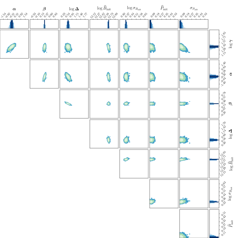
Figure 2: The power-law model – MCMC marginal parameter space. The 1D marginal distribution express the auto-scaled, normalised probability density ${\rm d}N/(N{\rm d}i)$ where $i$ is appropriate parameter according to the plot. On the 2D contour plot the colours represent the $1,2,3-\sigma$ levels. We constrained the range of the $\gamma$ posterior to zoom in on the populated part of the phase space.

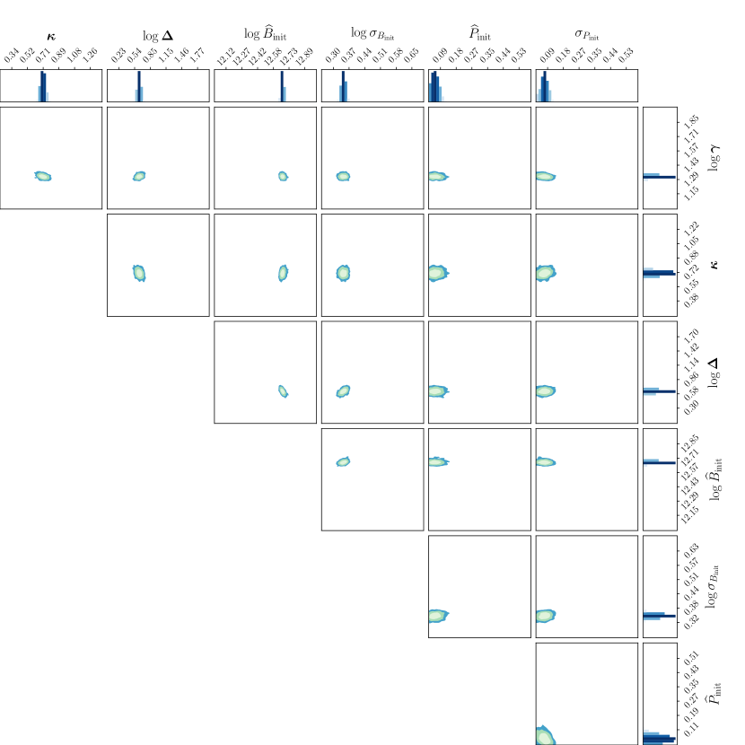
Figure 3: The rotational model – MCMC marginal parameter space. The 1D marginal distribution express the auto-scaled, normalised probability density ${\rm d}N/(N{\rm d}i)$ where $i$ is appropriate parameter according to the plot. On the 2D contour plot the colours represent the $1,2,3-\sigma$ levels. We constrained the range of the $\gamma$ posterior to zoom in on the populated part of the phase space.

The power-law model	The rotational model

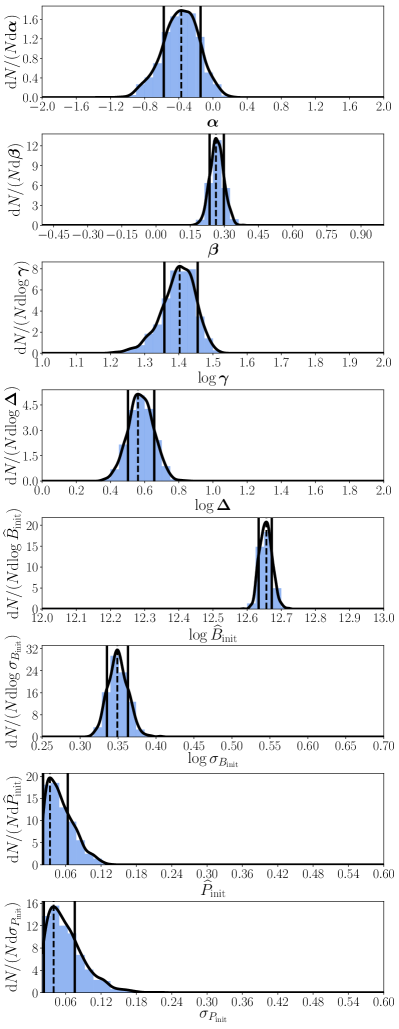
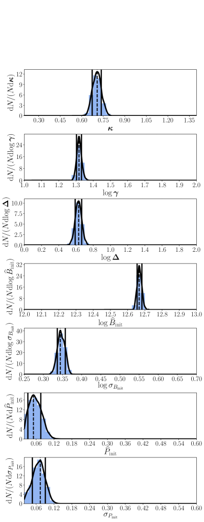
Figure 4: The comparison of the marginal distributions for both models. The 1-sigma level is derived by using Gaussian Kernel Density Estimation (black line) by integrating the probability from the Most Probable Value (dotted line). We constrained the range of the $\gamma$ posterior to zoom in on the populated part of the phase space.

4.1 The parameters marginal space

To visualize the multidimensional parameter space, we present one and two dimensional marginalised posterior distributions. The two dimensional results for power-law and rotational models are presented in Figures 2 and 3, respectively. The one-dimensional marginalised posterior distributions are shown in Figure 4.

4.1.1 The marginal distribution

The two-dimensional marginal probability distribution of the $i$-th and $j$-th parameters (denoted as $\mathcal{D}_{\theta_{ij}}$) is expressed by marginalizing the full-dimensional probability distribution $\mathcal{D}_{\bar{\theta}}$ upon all other parameters ($\Omega^{\prime}$ represents the parameter space excluding $i$-th and $j$-th dimensions):

$$\mathcal{D}_{\theta_{ij}}=\int_{\Omega^{\prime}}\mathcal{D}_{\bar{\theta}}{\rm d}\Omega^{\prime}$$ (26)

Similarly, the one-dimensional marginal distribution of the $i$-th parameter $\mathcal{D}_{\theta_{i}}$ is expressed by:

$$\mathcal{D}_{\theta_{i}}=\int_{\Omega^{\prime\prime}}\mathcal{D}_{\bar{\theta}}{\rm d}\Omega^{\prime\prime}$$ (27)

where $\Omega^{\prime\prime}$ represents the parameter space excluding all but the $i$-th dimension. To obtain the continuous probability density function ($\mathcal{C}_{\theta_{ij}}$ and $\mathcal{C}_{\theta_{i}}$) of the marginal distribution ($\mathcal{D}_{\theta_{ij}}$ and $\mathcal{D}_{\theta_{i}}$) we use the Gaussian kernel density estimation method (Scott, 2015) with a bandwidth $h$ (a function of number of points $n$ and dimensions $d$):

$$h(n,d)=n^{\frac{-1}{d+4}},$$ (28)

4.1.2 The most probable value and significance levels

We denote the most probable value (MPV) – the maximum of the marginal, continuous probability density function for each parameter (see Table 2). For confidence levels we use the $1,2,3-\sigma$ ranges corresponding to the $68.27$, $95.45$, and $99.73$ per cent of the distribution. The $\sigma$ ranges are computed by integrating the probability around the MPV.

Parameter	Most Probable Value
power-law model
${\alpha}$	$-0.37^{+0.22}_{-0.21}$
${\beta}$	$0.26^{+0.04}_{-0.02}$
$\log{\left(\gamma/{\rm mJy}\right)}$	$1.40^{+0.06}_{-0.04}$
$\log{\left(\Delta/{\rm Myr}\right)}$	$0.56^{+0.10}_{-0.06}$
$\log\left(\widehat{B}_{{\rm init}}/{\rm G}\right)$	$12.66^{+0.01}_{-0.03}$
$\log\left(\sigma_{B_{{\rm init}}}/{\rm G}\right)$	$0.35^{+0.01}_{-0.01}$
$\widehat{P}_{{\rm init}}\,{\rm s}$	$0.03^{+0.03}_{-0.01}$
$\sigma_{P_{{\rm init}}}\,{\rm s}$	$0.04^{+0.04}_{-0.02}$
rotational model
$\kappa$	$0.71^{+0.03}_{-0.04}$
$\log{\left(\gamma/{\rm mJy}\right)}$	$1.32^{+0.01}_{-0.02}$
$\log{\left(\Delta/{\rm Myr}\right)}$	$0.63^{+0.04}_{-0.04}$
$\log\left(\widehat{B}_{{\rm init}}/{\rm G}\right)$	$12.67^{+0.01}_{-0.02}$
$\log\left(\sigma_{B_{{\rm init}}}/{\rm G}\right)$	$0.34^{+0.02}_{-0.01}$
$\widehat{P}_{{\rm init}}\,{\rm s}$	$0.05^{+0.03}_{-0.02}$
$\sigma_{P_{{\rm init}}}\,{\rm s}$	$0.07^{+0.02}_{-0.02}$

Table 2: The most probable values (MPV) with one-$\sigma$ confidence level (the upper and lower limit). The $\alpha$, $\beta$, and $\kappa$ parameters are dimensionless.

4.1.3 Correlation coefficients

In the Table 3 we present the linear correlation coefficient $r$:

$$r=\frac{\sum^{n}_{i=1}(x_{i}-\bar{x})(y_{i}-\bar{y})}{\sqrt{\sum^{n}_{i=1}(x_{i}-\bar{x})^{2}}\sqrt{\sum^{n}_{i=1}(y_{i}-\bar{y})^{2}}}$$ (29)

for both models for each pair of the parameters, where $n$ is the number of chains in the final analysis.

The power-law model

The rotational model

Table 3: The linear correlation coefficient matrices. The colour represent the absolute value of correlation coefficients.

4.2 The resulting population

For both sets of the MPVs (for the power-law and rotational models) we computed a population of pulsars. We show the visible in the Parkes Multibeam Survey part of the population of the Figure 5. The method of presenting the pulsar density in two dimensional marginalisations of the comparison space ($P$-$\dot{P}$-$S$) is the final verification of the obtained results. As can be seen in the second row for the power-law model and in the third row of the Figure 5 for the rotational model, the fit of the modelled data to the observations can not be considered incorrect. We note that our simulation scheme always under estimates the data density – this behaviour can be seen as the pulsars density does not encompass the corresponding contour lines of the observations.

ATNF Catalogue

Power-law model

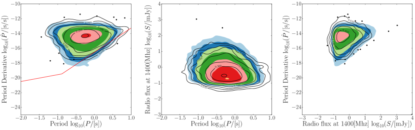
Rotational model

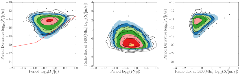
Figure 5: Observations – the subset of the ATNF catalogue (first row), power-law model (second row), and rotational model in the two-dimensional marginalisations of the comparison space $P$-$\dot{P}$-$S$. The colours indicate density levels for a given pair of dimensions $i$,$j$ (for e.g. $i=P$ and $j=\dot{P}$ for the first column). The contour lines relate to the observations in each plot. The dots represent observations that lay in the region with extremely low density.

5 Discussion

5.1 The model

5.1.1 Initial period distribution

We reached quite narrow initial period parameter distributions with most probable values equal to: $\hat{P}_{\rm init}\approx 0.03\,{\rm s}$ and $0.05\,{\rm s}$ for the power-law and rotational model, respectively. They both cover similar range of vales but the preferred mean value for the power-law model is significantly lower. In case of the standard deviation parameter of the initial period distribution we found out to be the most likely: $\sigma_{P_{\rm init}}\approx 0.03\,{\rm s}$ and $0.07\,{\rm s}$ for the power-law and rotational model, respectively.

The resulting distributions of initial periods in both cases are in agreement with the predictions made by Blondin & Mezzacappa (2007). However the hydrodynamic simulations lead to contradictory results (Rantsiou et al., 2011). In comparison to other population synthesis, in the works of Popov et al. (2010) they concluded that $\hat{P}_{\rm init}\approx 0.25\,{\rm s}$ with $\sigma_{P_{\rm init}}\approx 0.0001\,{\rm s}$, while Faucher-Giguère & Kaspi (2006) obtained the values $P_{\rm init}=0.3\,{\rm s}$ and $\sigma_{P_{\rm init}}=0.15\,{\rm s}$. The main difference between our results and Faucher-Giguère & Kaspi (2006) is the inclusion of magnetic field decay which can be interpreted as an accelerator for the pulsar movement on the $P$-$\dot{P}$ plane. Thus, the population can have faster initial periods as it evolves to the same final population. Moreover, Popov et al. (2010) included the magnetic field decay and reached similar values as Faucher-Giguère & Kaspi (2006). Therefore, we are convinced the discrepancy with previous results is due to better sampling of the parameter space. In particular, we evaluated a larger number of models and didn’t manually constrain the prior ranges.

5.1.2 Initial magnetic field distribution

The distribution of initial magnetic fields is almost identical in both models with the mean $\log B_{\rm init}\approx 12.66$ and $\log\sigma_{B_{\rm init}}\approx 0.34$). Those results are consistent with findings of Faucher-Giguère & Kaspi (2006) where they obtained ${\log}B_{\rm init}=12.65$ and $\sigma_{B_{\rm init}}=0.55$. In the work of Popov et al. (2010), authors reached larger value of the mean ${\log}B_{\rm init}=13.25$ with $\sigma_{B_{\rm init}}=0.6$. Such initial distribution of values means that no pulsar has initial field less then $\log B_{\rm init}\approx 11$. Such conclusion is consistent with the fact that if such pulsars with low magnetic field strength existed they would be clearly observable in the radio band. Furthermore, their evolution would be very slow which would increase their detection probability. The lack of observed pulsars in the region of $P\approx 0.1\,{\rm s}$ and $\dot{P}\approx 10^{-17}-10^{-18}\,{\rm ss}^{-1}$ implies that no quick spinning pulsars with magnetic field below $\log B_{\rm init}\approx 11$ are formed.

5.1.3 The rotational radio-emission model

In the rotational model we obtained the value of the exponent $\kappa$ in range between $0.67$ and $0.74$. Upon translating to $L_{\rm rot}$ (see eq. 7), we see that its exponent $\frac{1}{3}\kappa$ ranges from $0.22$ to $0.24$. This result disagrees with values obtained by Gullón et al. (2014) in the range from $0.45$ to $0.5$. We suspect that not including any radio switch-off mechanism (e.g. death lines) and limiting the comparison space to only $P$-$\dot{P}$ could play a significant role in the difference.

5.1.4 The power-law radio-emission model

We found the power-law exponents to be in range from $0.24$ to $0.30$ for the $\beta$ and from $-0.58$ to $-0.15$ for the $\alpha$. We see that our most probable values, $\alpha=-0.58$ and $\beta=0.26$, are in 2-$\sigma$ range of the results obtained by Bates et al. (2014): $\alpha=-1.12$ and $\beta=0.28$. In comparison with (Faucher-Giguère & Kaspi, 2006): $\alpha=-1.5$, $\beta=0.5$, we differ more than $3$ standard deviations. The difference can be explained by the inclusion of the magnetic field decay which does exhibit a strong correlation with other parameters describing the luminosity model (see Table 3 for $\alpha$, $\beta$, $\gamma$, and $\Delta$ parameters), and an improved sampling of the parameter space.

5.1.5 The fit of radio luminosity laws

Although the fit in the 2D marginal distributions of the comparison space (second and third column of the Figure 5) seems to be in general agreement with the observations, the comparison of the radio-flux distribution (see Figure 6) shows some discrepancies. Our models underestimates the lower radio-fluxes, and overestimates the brightest objects. Both models behave in the same way pointing to a possible systematic error in the method, or model description. The coupling of the $P$-$\dot{P}$-$S$ in both the optimisation (comparison space), period evolution and radio-luminosity law, may have degenerated the problem – leading to too few observational constraints with regard to the number of free parameters. We also note that the introduction a phenomenological death area (see eq. 14) might have altered the distribution of pulsars in the $P$-$\dot{P}$ plane (see Figure 5). We excluded the parameter $\Psi$ from our current analysis due to the complexity reduction of the computations. We plan to include the analysis of the death area in our future work.

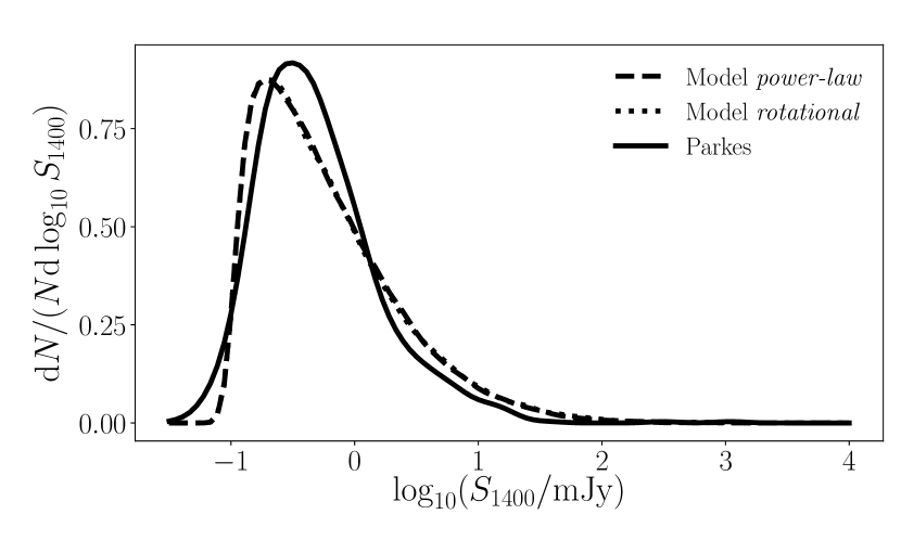
Figure 6: The comparison (upper plot) and difference (lower plot) of the distribution of the radio-flux of the observations, the power-law model, and the rotational model.

5.1.6 The kicks distribution

We are aware that Hobbs et al. (2005) may be an imperfect distribution of the SN kicks, as stated in Faucher-Giguère & Kaspi (2006) or more recently in Verbunt et al. (2017). However, the spatial distribution (see section 2.4.2 ) is beyond the scope of this work. Moreover, by employing the Parkes Multibeam Survey, we focus only on the Galactic disk towards the centre of the Galaxy (see Table 4), thus limiting our study to a younger subset of the whole Galactic population. Any possible discrepancies in the kicks model are neglected by this choice.

5.1.7 Pulsar ages

Figure 7: The cumulative distribution of the pulsars ages in the observed population. Lines – simulation limited to maximum age $t_{\rm{age}}=50\,{\rm{Myr}}$, Dots – simulation limited to maximum age $t_{\rm{age}}=200\,{\rm{Myr}}$

.

We found that, within our model, a fraction of less then $1\%$ of pulsars is older then $50\,{\rm Myr}$ (see Figure 7). Because those pulsars do not contribute in any significant way to the likelihood and as a result to MCMC and parameter estimation (a smaller 200-chains test yielded similar results to presented therein), we neglected this part of population. We limited the maximum age of pulsars to be $t_{\rm{age}}\leqslant 50\,{\rm Myr}$. We do not contradict the observed kinematic ages distribution (Noutsos et al., 2013). Our study is focused on the Galactic disk population (see Table 4) and we are unable to effectively compare with older kinematic-population. Moreover, by the inclusion of the magnetic field decay, we greatly speed up the pulsars evolution track on the $P$-$\dot{P}$ plane. This may lead to incorrect comparison between the evolution (simulation) age and the characteristic age distribution. By computing the characteristic age

$$\tau=\frac{P}{2\dot{P}},$$ (30)

we show in Figure 8 that the distribution of models resemble the observed sample and that it is possible to produce pulsars with $\tau{\geqslant}50\,{\rm Myr}$.

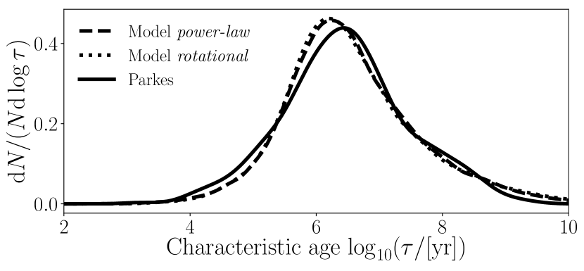
Figure 8: The probability density function of the characteristic age $\tau=P/(2\dot{P})$ in the reference ATNF subset for the Parkes Multibeam Survey and models.

Parameter	Symbol	Value	Unit
Receiver temperature	$T_{{\rm rec}}$	$24$	${\rm K}$
Bandwidth	$\Delta f$	$288$	${\rm MHz}$
Number of polarizations	$n_{{\rm p}}$	$2$	$1$
Frequency	$f$	$1400$	${\rm MHz}$
Sampling time	$\tau_{{\rm samp}}$	$0.00025$	${\rm s}$
Gain	$G$	$0.65$	${\rm K}/{\rm Jy}$
Integration time	$t_{{\rm i}}$	$2100$	${\rm s}$
Diagonal dispersion measure	${\rm DDM}$	27.61	${\rm pc}/{\rm cm}^{3}$
System loss	$\iota$	1.	1
Min. signal to noise ratio	$\left({\rm S/N}\right)_{{\rm min}}$	10.	1

The sky coverage Galactic longitude range $-100^{\circ}\leqslant l\leqslant 50^{\circ}$ Galactic latitude range $-5^{\circ}\leqslant b\leqslant 5^{\circ}$

Table 4: Parkes Multibeam Survey parameters.

5.1.8 Estimated SN rate

To derive the supernova rate from our models, we assume that the modelled and real populations have similar age ($t_{\rm max}=50\,{\rm Myr}$), and that the ratio of the number of visible pulsars $N_{\rm vis}$ to the total number of pulsars $N_{\rm tot}$ is constant:

$$\frac{N_{\rm vis}^{\rm real}}{N_{\rm tot}^{\rm real}}=\frac{N_{\rm vis}^{\rm model}}{N_{\rm tot}^{\rm model}},$$ (31)

where $N_{\rm vis}^{\rm model}$ is the number of visible pulsars in a given model equal to $60012$ and $58880$ for the power-law and rotational models respectively, the $N_{\rm tot}^{\rm model}$ is the total number of simulated pulsars equal to $5.e6$, the $N_{\rm vis}^{\rm real}$ is the observed sample of pulsars equal to $969$ pulsars, and the $N_{\rm tot}^{\rm real}$ is the total number of real pulsar and can be written as:

$$N_{\rm tot}^{\rm real}=t_{\rm max}r_{\rm SN}.$$ (32)

Where the $r_{SN}$ is the supernova rate per century. Thus, we obtain our estimate:

$$r_{\rm SN}=\frac{N_{\rm vis}^{\rm real}N_{\rm tot}^{\rm model}}{N_{\rm vis}^{\rm model}t_{\rm max}},$$ (33)

which yields:

$$r_{\rm SN}=\begin{cases}0.1615/100\,{\rm yr}&\text{{\em power-law} model}\\ 0.1646/100\,{\rm yr}&\text{{\em rotational} model}\end{cases}$$ (34)

Our estimate do not exceed the predicted rate of core-collapse supernova rate $0.5-1.1$ per century (van den Bergh & Tammann, 1991) as well the recent estimate based on INTEGRAL data for the combined type I b/c and type II supernova rate equal to $1.9\pm 1.1$ per century (Diehl et al., 2006).

5.1.9 The DM distribution

We limited our comparison space to three dimensions only – the period $P$ and its derivative $\dot{P}$ and the radio flux $S_{1400}$. Due to restriction on the computational time of the free electron distribution model of Yao et al. (2017) we excluded the geometrical part (galactic coordinates and dispersion measure) from our comparison space. Therefore we do not draw any conclusion about the pulsars spatial distribution in the Milky Way and their initial kicks, but the distances (in our case the dispersion measure) can have implication for the radio luminosity model. We present the model distribution of the dispersion measure and the one of the Parkes Multibeam Survey in Figure 9. The model distribution and the observed one are close even though they were not fitted.

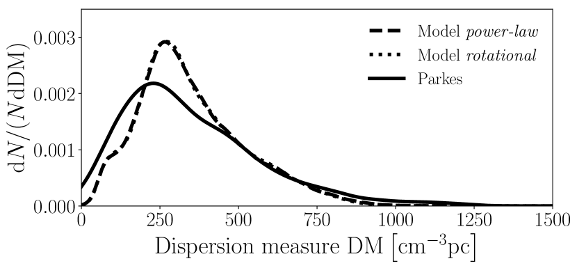
Figure 9: The probability density function of the dispersion measure in the reference ATNF subset for the Parkes Multibeam Survey and models.

5.2 Pulsar population with Square Kilometre Array

A very interesting consequence of the modelling presented here is the possibility to extend the results to the population of pulsars observable by the Square Kilometre Array (SKA). The SKA telescope is described in Carilli & Rawlings (2004), Staff & Array (2015), Kramer & Stappers (2015), and Grainge et al. (2017). We present the extrapolation of the observable pulsar population using the two models of pulsar luminosity considered above (the power-law model and rotational one) with their parameters set to the most probable values (see Table 2). We list two sets of probable parameters that describe the SKA for a mid-frequency survey in Table 5. The first one SKA-1-Mid represents our estimate of the initially planned SKA operation and the SKA-1-Mid-B a more pragmatic view of the parameters.

Parameter	Symbol	Value	Unit
Receiver temperature	$T_{{\rm rec}}$	$30$	${\rm K}$
Bandwidth	$\Delta f$	$300$	${\rm MHz}$
Number of polarizations	$n_{{\rm p}}$	$2$	$1$
Frequency	$f$	$1400$	${\rm MHz}$
Sampling time	$\tau_{{\rm sampling}}$	$0.000064$	${\rm s}$
Gain	$G$	$15$ ($2$)	${\rm K}/{\rm Jy}$
Integration time	$t_{{\rm i}}$	$2100$	${\rm s}$
Diagonal dispersion measure	${\rm DDM}$	289.49	${\rm pc}/{\rm cm}^{3}$
System loss	$\beta$	1.	1
Min. signal to noise ratio	$\left({\rm S/N}\right)_{{\rm min}}$	10.	1

Table 5: SKA-1-Mid and SKA-1-Mid-B (in brackets) survey parameters.

To perform the extrapolation we compute a pulsar population of a given size ($10^{7}$) for the best set of parameters for both models. We infer what part of this population is seen in each survey (Parkes Multibeam, SKA-1-Mid, and SKA-1-Mid-B). We then compare the ratio of modelled pulsars seen in the Parkes Multibeam Survey to the cardinality of used subsection of the ATNF catalogue. This ratio is considered the normalisation constant $W$. In order to scale the artificial SKA observation we restrict the SKA-1-Mid and SKA-1-Mid-B surveys to the same part of the sky as the Parkes Multibeam Survey. Upon scaling the SKA surveys with the normalisation constant $W$ we reach the estimated number of detectable single pulsars. We present the distribution of the detectable pulsars in the function of the radio-flux at Figure 10. By our estimate, should the SKA observatory perform a survey of the same part of sky as the Parkes Mutlibeam Survey, we would reach an increase in detected radio pulsars by $23\%$ or $137\%$ for the SKA-1-Mid-B and SKA-1-Mid survey, respectively.

The power-law model

The rotational model

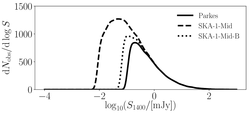
Figure 10: The distribution of pulsars radio-fluxes in the Parkes Multibeam Survey and the prediction for the SKA-1-Mid and SKA-1-Mid-B surveys. The total number of pulsars in $N_{\rm obs}$ is equal to $969$ for Parkes with our selection cuts. In case of the SKA surveys the number of pulsars is $2364$ and $2285$ for the power-law and rotational model, respectively. For the low-cost SKA survey the number of pulsar is almost the same $1241$ and $1229$ for the power-law and rotational model, respectively.

6 Conclusions

We presented a radio pulsar population synthesis model based on the one described by Faucher-Giguère & Kaspi (2006). We compared it with observations using the likelihood statistic and we used the Markov Chain Monte Carlo method to explore the parameter space. We used the recent model for the computation of the interstellar medium by Yao et al. (2017). We compared the model with observations in the space spanned by period, period derivative, and radio flux. The pulsar initial parameters and their evolution are described by five parameters. We have explored two models with two different parametrizations of the pulsar luminosity: the power-law model described by three additional parameters and the rotational model described by two parameters. This allowed us to the estimation of the parameters and their confidence level. We found that the magnetic field decay is scale quite short and is approximately $3.63^{+0.94}_{-0.47}\,{\rm Myr}$ in the power-law or $4.27^{+0.4}_{-0.38}\,{\rm Myr}$ in the rotational model. The initial period distributions are centred around $\hat{P}_{\rm init}\approx 30\,{\rm ms}$ and $50\,{\rm ms}$ with widths of $\sigma_{P_{\rm init}}\approx 40\,{\rm ms}$ and $70$ for the power-law and rotational model, respectively. The initial distribution of logarithm of magnetic field is almost identical in both models with the average $\log B_{\rm init}\approx 12.66$ and $\log\sigma_{B_{\rm init}}\approx 0.35$. We found that the preferred values of the exponents for the power-law radio-luminosity model are $\alpha=-0.37^{+0.22}_{-0.21}$ and $\beta=0.26^{+0.04}_{-0.02}$, and for the model proportional to the rotational energy loss is $\kappa=0.71^{+0.03}_{-0.04}$. Proposed parameters values differ from the works of Faucher-Giguère & Kaspi (2006), Popov et al. (2010), Gullón et al. (2014), and Bates et al. (2014). We contribute the difference to the inclusion of the radio-flux in the space that the main statistic (used to optimize the model) used as well as significantly large scope of the simulations (due to the increase of the available computational power).

In the view of the significant linear correlation between parameters exhibited by the power-law model, and the fact that two models lead to an almost identical population of observed pulsars, we believe that the rotational model should be preferred. We note, that even the rotational model has some non-negligible correlation between magnetic field decay time-scale and parameters describing the initial distribution of magnetic field. To shed some light on the possible cause of the parameters correlation, additional constraints from the observation should be provided, and more sophisticated description of the radio luminosity implemented.

We estimated the number of new observable pulsars, should the SKA survey cover the same area, as the Parkes Multibeam Survey to be increased by $23-137\%$ depending on the final parameters of the SKA survey. We release the Indri code used in this research in hopes of contributing to the advancement of dynamical models in the pulsar population synthesis research field.

Appendix A

In this appendix, for the completion purpose, we present the parts of the model that are identical to the model developed by Faucher-Giguère & Kaspi (2006).

A.1 The Milky Way

A.1.1 The Galactic potential

We use the well-established three-component Galactic potential consisting of the disk, the bulge and the halo. The bulge $\Phi_{{\rm{Bulge}}}$ and the disk $\Phi_{{\rm{Disk}}}$ gravitational potentials are adopted after Miyamoto & Nagai (1975). The formula describing the bulge is:

$$\Phi_{{\rm{Bulge}}}=-\frac{GM_{b}}{\sqrt{b_{b}^{2}+r^{2}}}$$ (35)

where $M_{b}=1.12\times 10^{10}\,{\rm M}_{\odot}$ and $b_{b}=0.277\,{\rm kpc}$, and $r=(x^{2}+y^{2}+z^{2})^{1/2}$. We model the disk potential as:

$$\Phi_{{\rm{Disk}}}=-\frac{GM_{d}}{\sqrt{{\left(a_{d}+\sqrt{b_{d}^{2}+z^{2}}\right)}^{2}+\rho^{2}}}$$ (36)

where $M_{d}=8.78\times 10^{10}\,{\rm M}_{\odot}$, $a_{d}=4.2\,{\rm kpc}$ and $b_{d}=0.198\,{\rm kpc}$, and $\rho=(x^{2}+y^{2})^{1/2}$. We use the halo potential $\Phi_{{\rm{Halo}}}$ following the model of Paczynski (1990):

$$\Phi_{{\rm{Halo}}}=-\frac{GM_{h}}{2r_{c}}{\left(2\frac{r_{c}}{r}\arctan\left(\frac{r}{r_{c}}\right)+\log\left(\frac{r^{2}}{r_{c}^{2}}+1\right)\right)}$$ (37)

where $M_{h}=5\times 10^{10}\,{\rm M}_{\odot}$ $r_{c}=6\,{\rm kpc}$. As the associated density of the halo is diverging so we cut the halo potential at $r_{cut}=100\,{\rm kpc}$, see e.g. Belczynski et al. (2010). We neglect the dependence of the galactic potential on the individual Galactic arms.

A.1.2 The initial positions of pulsars

Arm	$k\,{\rm rad}$	$\rho_{0}\,{\rm kpc}$	$\theta_{0}\,{\rm rad}$
Norma	$4.25$	$3.48$	$1.57$
Carina-Sagittarius	$4.25$	$3.48$	$4.71$
Perseus	$4.89$	$4.90$	$4.05$
Crux-Scutum	$4.89$	$4.90$	$0.95$

Table 6: Spiral arms parameters.

We adopt the initial position distribution after Faucher-Giguère & Kaspi (2006) with the assumption that pulsars are born inside the galactic spiral arms. Following them, we exclude the Local Arm as the origin of the pulsars. The centroids of each arm are described as logarithmic spirals (Wainscoat et al., 1992):

$$\theta(\rho)=k\log\left(\frac{\rho}{\rho_{0}}\right)+\theta_{0}$$ (38)

with their parameters listed in the Table 6. With equal probability we chose the arm in which pulsar is born. The distance $\rho_{{\rm raw}}$ from the centre of the Galaxy is drawn using the stellar surface density distribution in the Galactic plane (Yusifov & Küçük, 2004):

$$\xi(\rho_{{\rm raw}})\sim\left(\frac{\rho_{{\rm raw}}+R_{1}}{R_{\odot}+R_{1}}\right)^{a}\exp\left(-b\left(\frac{\rho_{{\rm raw}}-R_{\odot}}{R_{\odot}+R_{1}}\right)\right)$$ (39)

where $a=1.64$, $b=4.01$, $R_{1}=0.55\,{\rm kpc}$, and $R_{\odot}=8.5\,{\rm kpc}$ is the distance of the Sun from the Galactic centre. We insert the radial distance into equation 38 to obtain the position along the spiral arm’s centroid $(\rho_{{\rm raw}},\theta_{{\rm raw}})$. This position is then smeared by adding a correction to the angle $\theta_{{\rm raw}}$ to avoid artificial structures in the Galactic centre:

$$\theta_{{\rm wide}}=\theta_{{\rm raw}}+\theta_{{\rm corr}}\exp{\frac{-0.35\rho_{{\rm raw}}}{{\rm kpc}}}$$ (40)

where $\theta_{{\rm corr}}$ is randomly chosen from the interval of $[0,2\pi)$ radians. We introduce the internal structure of spiral arms by displacing the initial radial position of the pulsar in the galactic plane. We add a vector with random direction and a length drawn from a Gaussian distribution with $\sigma=0.07\rho_{{\rm raw}}$. The resulting initial position distribution in the Galactic plane is shown in the Figure 11. The vertical position of the pulsar is drawn from the exponential distribution with the mean $\left<z_{0}\right>=0.05\,{\rm kpc}$. We populate the Galaxy with stars by rotating spiral arms and inserting pulsars uniformly in time from their maximal simulated age, $\max(t_{\rm age})=50\,{\rm Myr}$ ago, to a present day. We assume a simple, rigid Galactic rotation with the period of $P_{\rm rot}=250\,{\rm Myr}$:

$$\theta=\theta_{{\rm wide}}-2\pi t_{\rm age}/P_{\rm rot}$$ (41)

We justify the rigid rotation assumption with the maximum possible age of a modelled pulsar $\max(t_{\rm age})=50\,{\rm Myr}$ being significantly lower then the rotation period of the Galaxy. For the discussion of this assumption see section 5.1.7.

Figure 11: Spiral Arms – initial positions distribution in the Galactic plane of randomly drawn, $10^{7}$ pulsars.

A.1.3 The initial velocity

At birth, each pulsar is subjugated to a kick due to the supernova explosion resulting in change in the initial velocity. We use the model of Hobbs et al. (2005) to draw the absolute value of the kicks velocity from a one-dimensional Maxwellian distribution with a mean $\left<v\right>=265\,{\rm km/s}$:

$$\mathcal{P}_{{\rm kick}}(v)=\sqrt{\frac{2}{\pi}}\frac{v^{2}}{\left<v\right>^{3}}\exp\left(\frac{-v^{2}}{2\left<v\right>^{2}}\right)$$ (42)

and a random direction. For the uniform spherical distribution of points we employ the algorithm of Marsaglia (1972). The resulting kick vector is added to the Keplerian motion in the Galactic potential at the neutron stars birth position.

A.2 The neutron star physics

A.2.1 The rotation evolution

To describe the spin-down process we use the canonical lighthouse model (Ostriker & Gunn, 1969). It approximates the pulsar with magnetic dipole rotating in a vacuum and assumes that the total loss of the rotation energy is emitted in the electromagnetic spectrum. This leads to the following relation between magnetic field induction, period and period derivative (for details refer to Shapiro & Teukolsky (1986) chapter 10.5):

$$B=\left({\frac{3Ic^{3}P\dot{P}}{8\pi^{2}R^{6}_{{\rm NS}}}}\right)^{1/2}=\eta(P\dot{P})^{1/2}$$ (43)

for a perpendicular rotator, where $\eta\simeq 3.2\times 10^{19}\,{\rm G}\,{\rm s}^{-1/2}$.

A.2.2 The initial parameters of pulsars

We adopted initial spin period distribution and magnetic field strength from the optimal model by Faucher-Giguère & Kaspi (2006). In case of the period it is a positive normal distribution (we redraw negative values) centred at $\widehat{P}_{\rm init}$ and with standard deviation $\sigma_{P_{\rm init}}$. We initialise the magnetic field strength with values drawn from log-normal distribution centred at a value of $\log(\widehat{B}_{\rm init})$ and with standard deviation $\log(\sigma_{B_{\rm init}})$. All four variables presented above are used to parametrize the evolution model. We list their limits in the Table 1.

A.3 Radio Properties

A.3.1 The minimal detectable flux

We follow identical prescription as Osłowski et al. (2011) to model radio selection effects. The minimal detectable flux of a pulsar is described by the radiometer equation (Dewey et al., 1985) adjusted for pulsating sources:

$$S_{{\rm min}}=\frac{\iota\left({\rm S/N}\right)_{{\rm min}}T_{{\rm sys}}}{G\sqrt{n_{{\rm p}}t_{{\rm i}}\Delta f}}\sqrt{\frac{W_{\rm e}}{P-W_{\rm e}}}$$ (44)

where the $\iota$ is a value describing system loss, $T_{\rm sys}$ is the system temperature, $G$ is the gain, $n_{\rm p}$ represents the number of polarizations, ${\Delta}f$ is the bandwidth, $t_{\rm i}$ is the integration time, $({\rm S/N})_{\rm min}$ represents the minimal signal to noise ratio, $W_{\rm e}$ is the effective width of the pulse and $P$ is the pulsar spin period. We supply the formula with values appropriate to the Parkes Multibeam Survey (see Table 4). For the system temperature $T_{\rm sys}$ we consider only the sky temperature $T_{\rm sky}$ in the direction of the measurement and the receiver noise temperatures $T_{\rm rec}$:

$$T_{{\rm sys}}=T_{{\rm rec}}+T_{{\rm sky}}$$ (45)

The effective width of the pulse $W_{\rm e}$ is a function of the intrinsic width $W_{\rm i}$, the sampling time $\tau_{\rm samp}$, the pulsar dispersion measure ${\rm DM}$, the diagonal dispersion measure ${\rm DDM}$ (characteristic to the survey) and the interstellar scattering time $\tau_{{\rm scatt}}$ describing the pulse widening due to the multipath propagation (dissipation of the signal by the free electron clouds in the Galaxy). The effective width $W_{\rm e}$ formula takes form of:

$$W_{{\rm e}}^{2}=W_{{\rm i}}^{2}+\tau_{{\rm samp}}^{2}+\left(\tau_{{\rm samp}}\frac{{\rm DM}}{{\rm DDM}}\right)^{2}+\tau_{{\rm scatt}}^{2}$$ (46)

We obtained the interstellar scattering time $\tau_{\rm scatt}$ using the model developed by Bhat et al. (2004) in which $\tau_{{\rm scatt}}$ is a function of the dispersion measure ${\rm DM}$. The minimal flux $S_{{\rm min}}$, the effective width $W_{\rm e}$, the system temperature $T_{{\rm sys}}$ and $\tau_{{\rm scattering}}$ were calculated using the functions from the PSREVOLVE code developed at the Centre for Astrophysics and Supercomputing, Swinburne University of Technology.

References

- Arzoumanian et al. (2002) Arzoumanian Z., Chernoff D. F., Cordes J. M., 2002, ApJ, 568, 289
- Bates et al. (2014) Bates S. D., Lorimer D. R., Rane A., Swiggum J., 2014, MNRAS, 439, 2893
- Belczynski et al. (2010) Belczynski K., Benacquista M., Bulik T., 2010, ApJ, 725, 816
- Beskin et al. (2015) Beskin V. S., Chernov S. V., Gwinn C. R., Tchekhovskoy A. A., 2015, Space Sci. Rev., 191, 207
- Bhat et al. (2004) Bhat N. D. R., Cordes J. M., Camilo F., Nice D. J., Lorimer D. R., 2004, ApJ, 605, 759
- Blondin & Mezzacappa (2007) Blondin J. M., Mezzacappa A., 2007, Nature, 445, 58
- Carilli & Rawlings (2004) Carilli C. L., Rawlings S., 2004, New Astron. Rev., 48, 979
- Cordes & Lazio (2002) Cordes J. M., Lazio T. J. W., 2002, ArXiv Astrophysics e-prints
- Cordes & Lazio (2003) Cordes J. M., Lazio T. J. W., 2003, ArXiv Astrophysics e-prints
- Dewey et al. (1985) Dewey R. J., Taylor J. H., Weisberg J. M., Stokes G. H., 1985, ApJ, 294, L25
- Diehl et al. (2006) Diehl R., et al., 2006, Nature, 439, 45
- Faucher-Giguère & Kaspi (2006) Faucher-Giguère C.-A., Kaspi V. M., 2006, ApJ, 643, 332
- Foreman-Mackey et al. (2013) Foreman-Mackey D., Hogg D. W., Lang D., Goodman J., 2013, PASP, 125, 306
- Gilks et al. (1995) Gilks W. R., Best N., Tan K., 1995, Applied Statistics, pp 455–472
- Gold (1968) Gold T., 1968, Nature, 218, 731
- Gonthier et al. (2007) Gonthier P. L., Story S. A., Clow B. D., Harding A. K., 2007, Ap&SS, 309, 245
- Goodman & Weare (2010) Goodman J., Weare J., 2010, Communications in Applied Mathematics and Computational Science, Vol.~5, No.~1, p.~65-80, 2010, 5, 65
- Grainge et al. (2017) Grainge K., et al., 2017, Astronomy Reports, 61, 288
- Gullón et al. (2014) Gullón M., Miralles J. A., Viganò D., Pons J. A., 2014, MNRAS, 443, 1891
- Hastings (1970) Hastings W. K., 1970, Biometrika, 57, 97
- Hewish et al. (1969) Hewish A., Bell S. J., Pilkington J. D. H., Scott P. F., Collins R. A., 1969, Nature, 224, 472
- Hobbs et al. (2005) Hobbs G., Lorimer D. R., Lyne A. G., Kramer M., 2005, MNRAS, 360, 974
- Igoshev & Popov (2015) Igoshev A. P., Popov S. B., 2015, Astronomische Nachrichten, 336, 831
- Kiel & Hurley (2009) Kiel P. D., Hurley J. R., 2009, MNRAS, 395, 2326
- Kiel et al. (2008) Kiel P. D., Hurley J. R., Bailes M., Murray J. R., 2008, MNRAS, 388, 393
- Kramer & Stappers (2015) Kramer M., Stappers B., 2015, Advancing Astrophysics with the Square Kilometre Array (AASKA14), p. 36
- Levin et al. (2013) Levin L., et al., 2013, MNRAS, 434, 1387
- Lorimer (2011) Lorimer D. R., 2011, in Torres D. F., Rea N., eds, High-Energy Emission from Pulsars and their Systems. p. 21 (arXiv:1008.1928), doi:10.1007/978-3-642-17251-9_2, http://adsabs.harvard.edu/abs/2011heep.conf...21L
- MacKay (2003) MacKay D., 2003, Information Theory, Inference and Learning Algorithms. Cambridge University Press
- Manchester et al. (2001) Manchester R. N., et al., 2001, MNRAS, 328, 17
- Manchester et al. (2005) Manchester R. N., Hobbs G. B., Teoh A., Hobbs M., 2005, AJ, 129, 1993
- Maron et al. (2000) Maron O., Kijak J., Kramer M., Wielebinski R., 2000, A&AS, 147, 195
- Marsaglia (1972) Marsaglia G., 1972, Ann. Math. Statist., 43, 645
- Matsumoto & Nishimura (1998) Matsumoto M., Nishimura T., 1998, ACM Trans. Model. Comput. Simul., 8, 3
- Miyamoto & Nagai (1975) Miyamoto M., Nagai R., 1975, PASJ, 27, 533
- Mosegaard & Tarantola (1995) Mosegaard K., Tarantola A., 1995, J. Geophys. Res., 100, 12
- Narayan & Ostriker (1990) Narayan R., Ostriker J. P., 1990, ApJ, 352, 222
- Noutsos et al. (2013) Noutsos A., Schnitzeler D. H. F. M., Keane E. F., Kramer M., Johnston S., 2013, MNRAS, 430, 2281
- Osłowski et al. (2011) Osłowski S., Bulik T., Gondek-Rosińska D., Belczyński K., 2011, MNRAS, 413, 461
- Ostriker & Gunn (1969) Ostriker J. P., Gunn J. E., 1969, ApJ, 157, 1395
- Pacini (1967) Pacini F., 1967, Nature, 216, 567
- Paczynski (1990) Paczynski B., 1990, ApJ, 348, 485
- Popov & Prokhorov (2007) Popov S. B., Prokhorov M. E., 2007, Physics Uspekhi, 50, 1123
- Popov et al. (2010) Popov S. B., Pons J. A., Miralles J. A., Boldin P. A., Posselt B., 2010, MNRAS, 401, 2675
- Rantsiou et al. (2011) Rantsiou E., Burrows A., Nordhaus J., Almgren A., 2011, ApJ, 732, 57
- Rudak & Ritter (1994) Rudak B., Ritter H., 1994, MNRAS, 267, 513
- Scott (2015) Scott D. W., 2015. John Wiley & Sons
- Shapiro & Teukolsky (1986) Shapiro S. L., Teukolsky S. A., 1986, Black Holes, White Dwarfs and Neutron Stars: The Physics of Compact Objects. http://adsabs.harvard.edu/abs/1986bhwd.book.....S
- Sharma (2017) Sharma S., 2017, ARA&A, 55, 213
- Staff & Array (2015) Staff S. O., Array S., 2015, Advancing Astrophysics with the Square Kilometer Array. Dolman Scott Limited
- Tarantola (2005) Tarantola A., 2005, Inverse Problem Theory and Methods for Model Parameter Estimation. EngineeringPro collection, Society for Industrial and Applied Mathematics
- Tauris & Manchester (1998) Tauris T. M., Manchester R. N., 1998, MNRAS, 298, 625
- Verbunt et al. (2017) Verbunt F., Igoshev A., Cator E., 2017, A&A, 608, A57
- Verlet (1967) Verlet L., 1967, Physical Review, 159, 98
- Wainscoat et al. (1992) Wainscoat R. J., Cohen M., Volk K., Walker H. J., Schwartz D. E., 1992, ApJS, 83, 111
- Yao et al. (2017) Yao J. M., Manchester R. N., Wang N., 2017, ApJ, 835, 29
- Yusifov & Küçük (2004) Yusifov I., Küçük I., 2004, A&A, 422, 545
- Zhang & Kojima (2006) Zhang C. M., Kojima Y., 2006, MNRAS, 366, 137
- van den Bergh & Tammann (1991) van den Bergh S., Tammann G. A., 1991, ARA&A, 29, 363