Study of a chemo-repulsion model with quadratic production. Part I: Analysis of the continuous problem and time-discrete numerical schemes

Abstract

We consider a chemo-repulsion model with quadratic production in a bounded domain. Firstly, we obtain global in time weak solutions, and give a regularity criterion (which is satisfied for $1D$ and $2D$ domains) to deduce uniqueness and global regularity. After, we study two cell-conservative and unconditionally energy-stable first-order time schemes: a (nonlinear and positive) Backward Euler scheme and a linearized coupled version, proving solvability, convergence towards weak solutions and error estimates. In particular, the linear scheme does not preserve positivity and the uniqueness of the nonlinear scheme is proved assuming small time step with respect to a strong norm of the discrete solution. This hypothesis is reduced to small time step in $nD$ domains ($n\leq 2$) where global in time strong estimates are proved. Finally, we show the behavior of the schemes through some numerical simulations.

2010 Mathematics Subject Classification. 35K51, 35Q92, 65M12, 65M15, 92C17.

Keywords: Chemo-repulsion model, quadratic production, first-order time schemes, energy-stability, convergence, error estimates.

1 Introduction

Chemotaxis is understood as the biological process of the movement of living organisms in response to a chemical stimulus which can be given towards a higher (attractive) or lower (repulsive) concentration of a chemical substance. At the same time, the presence of living organisms can produce or consume chemical substance. A chemo-repulsive model with generic production can be given by the following parabolic PDE’s system:

$$\left\{\begin{array}[c]{lll}\partial_{t}u-\Delta u=\nabla\cdot(u\nabla v)\quad\mbox{in}\ \Omega,\ t>0,\\ \partial_{t}v-\Delta v+v=f(u)\quad\mbox{in}\ \Omega,\ t>0,\end{array}\right.$$ (1)

where $\Omega\subset\mathbb{R}^{d}$, $d=2,3$, is an open bounded domain with boundary $\partial\Omega$. The unknowns for this model are $u(\boldsymbol{x},t)\geq 0$, the cell density, and $v(\boldsymbol{x},t)\geq 0$, the chemical concentration. Moreover, $f(u)$ is a function which is nonnegative for any $u\geq 0$. In this paper, we consider the particular case in which the production term is quadratic, that is $f(u)=u^{2}$, and then we focus on the following initial-boundary value problem:

$$\left\{\begin{array}[c]{lll}\partial_{t}u-\Delta u=\nabla\cdot(u\nabla v)\quad\mbox{in}\ \Omega,\ t>0,\\ \partial_{t}v-\Delta v+v=u^{2}\quad\mbox{in}\ \Omega,\ t>0,\\ \displaystyle\frac{\partial u}{\partial\boldsymbol{n}}=\frac{\partial v}{\partial\boldsymbol{n}}=0\ \ \mbox{on}\ \partial\Omega,\ t>0,\\ u(\boldsymbol{x},0)=u_{0}(\boldsymbol{x})\geq 0,\ v(\boldsymbol{x},0)=v_{0}(\boldsymbol{x})\geq 0\ \ \mbox{in}\ \Omega.\end{array}\right.$$ (2)

In the case of linear production, that is $f(u)=u$, model (1) is well-posed in the following sense ([3]): there exist global in time weak solutions (based on an energy inequality) and, for $1D$ and $2D$ domains, there exists a unique global in time strong solution. However, it is interesting to analyze the case of nonlinear production which is justified biologicaly when the process of signal production through cells need no longer dependence on the population density in a linear manner, for instance when saturation effects at large (or short) densities are taken into account (see [20] and references therein). In particular, we focus in model (2) because the quadratic production term allows to control an energy in $L^{2}(\Omega)$-norm for $u$ (see (24)-(25)), which is very useful for performing numerical analysis; and, as far as we know, there are not works studying problem (2).

The aim of this paper is twofold; first to obtain existence of global in time weak solution, which is unique and regular in $1D$ and $2D$ domains, and second to design two energy-stable time-discrete schemes approaching model (2). Some other properties like solvability, positivity, convergence towards weak solutions and error estimates will be studied.

There are some works about numerical analysis for chemotaxis models. For instance, for the Keller-Segel system (i.e. with chemo-attraction and linear production), in [8] it was studied the convergence of a finite volume scheme. Some error estimates were proved for a fully discrete discontinuous Finite Element (FE) method in [6]. In [4], the nonnegativity of numerical solutions to a generalized Keller-Segel model was analyzed. A mixed FE approximation was studied in [14]; and in [16, 17], were proved error estimates for a conservative FE approximation. In [10], the authors studied unconditionally energy stable fully discrete FE schemes for a chemo-repulsion model with linear production. The convergence of a combined finite volume-nonconforming FE scheme was studied in [2], in the case where the chemotaxis occurs in heterogeneous medium. In [21], the convergence of a mass-conservative characteristic FE method was studied and some error estimates were proved.

In order to develop our analysis, we reformulate (2) by introducing the auxiliary variable ${\boldsymbol{\sigma}}=\nabla v$. Then, the model (2) is rewritten as follows:

$$\left\{\begin{array}[c]{lll}\partial_{t}u-\nabla\cdot(\nabla u)=\nabla\cdot(u{\boldsymbol{\sigma}})\quad\mbox{in}\ \Omega,\ t>0,\\ \partial_{t}{\boldsymbol{\sigma}}-\nabla(\nabla\cdot{\boldsymbol{\sigma}})+\mbox{rot}(\mbox{rot }{\boldsymbol{\sigma}})+{\boldsymbol{\sigma}}=\nabla(u^{2})\quad\mbox{in}\ \Omega,\ t>0,\\ \displaystyle\frac{\partial u}{\partial\boldsymbol{n}}=0\quad\mbox{on}\ \partial\Omega,\ t>0,\\ {\boldsymbol{\sigma}}\cdot\boldsymbol{n}=0,\ \ \left[\mbox{rot }{\boldsymbol{\sigma}}\times\boldsymbol{n}\right]_{tang}=0\quad\mbox{on}\ \partial\Omega,\ t>0,\\ u(\boldsymbol{x},0)=u_{0}(\boldsymbol{x})\geq 0,\ {\boldsymbol{\sigma}}(\boldsymbol{x},0)=\nabla v_{0}(\boldsymbol{x})\quad\mbox{in}\ \Omega,\end{array}\right.$$ (3)

where (3)₂ is obtained by applying the gradient operator to equation (2)₂ and adding the term $\mbox{rot}(\mbox{rot }{\boldsymbol{\sigma}})$ using the fact that $\mbox{rot }{\boldsymbol{\sigma}}=\mbox{rot}(\nabla v)=0$. Once solved (3), $v$ can be recovered from $u^{2}$ solving

$$\left\{\begin{array}[c]{lll}\partial_{t}v-\Delta v+v=u^{2}\quad\mbox{in}\ \Omega,\ t>0,\\ \displaystyle\frac{\partial v}{\partial\boldsymbol{n}}=0\quad\mbox{on}\ \partial\Omega,\ t>0,\\ v(\boldsymbol{x},0)=v_{0}(\boldsymbol{x})\geq 0\quad\mbox{in}\ \Omega.\end{array}\right.$$ (4)

The use of the variable ${\boldsymbol{\sigma}}$ let simplify the notation throughout the paper. On the other hand, the role of ${\boldsymbol{\sigma}}$ will be different for fully discrete schemes where problem (2) and (3)-(4) are not equivalent. In fact, as will be analyzed in the forthcoming paper [9], by using a FE spatial discretization it will be very convenient to use the variables $(u,{\boldsymbol{\sigma}})$ in order to obtain an unconditionally energy-stable scheme.

The outline of this paper is as follows. In Section 2, the notation and preliminary results are given. In Section 3, the continuous problem (2) is analyzed, defining the concept of global in time weak solutions, and obtaining global in time strong regularity of the model by assuming the regularity criterion (38), which is satisfied for $1D$ and $2D$ domains. In Section 4, the Backward Euler scheme corresponding to problem (3)-(4) is analyzed, including cell-conservation, unconditional energy-stability, solvability, positivity and error estimates of the scheme. In particular, uniqueness of solution of the scheme is proved under a hypothesis that assumes small time step multiplied by a strong norm of the scheme (the discrete version of (38)), which can be simplified in the case of $1D$ and $2D$ domains where strong estimates are obtained for the scheme. Moreover, the existence of weak solutions of model (2) is proved throughout the convergence of this scheme when the time step goes to $0$. In Section 5, a linearized coupled scheme for model (3)-(4) is proposed, and again some properties of this linear scheme are analyzed, comparing to the previous nonlinear scheme. Finally, in Section 6, some numerical simulations using FE approximations associated to both time schemes are shown, in order to verify numerically the theoretical results obtained in terms of positivity and unconditional energy-stability.

2 Notations and preliminary results

Recall some functional spaces which will be used throughout this paper. We consider the Lebesgue spaces $L^{p}(\Omega)$, $1\leq p\leq\infty$, and the Sobolev spaces $H^{m}(\Omega)$, by denoting their norms by $\|\cdot\|_{L^{p}}$ and $\|\cdot\|_{m}$, respectively. In particular, the $L^{2}(\Omega)$-norm will be represented by $\|\cdot\|_{0}$. Corresponding Sobolev spaces of vector valued functions will be denoted by $\boldsymbol{H}^{1}(\Omega)$, $\boldsymbol{L}^{2}(\Omega),$ and so on; and we consider the vectorial space

$$\boldsymbol{H}^{1}_{\sigma}(\Omega):=\{\boldsymbol{\sigma}\in\boldsymbol{H}^{1}(\Omega);\boldsymbol{\sigma}\cdot\boldsymbol{n}=0\mbox{ on }\partial\Omega\}.$$

The following norms are equivalent in $H^{1}(\Omega)$, $H^{2}(\Omega)$ ([15]) and $\boldsymbol{H}_{\sigma}^{1}(\Omega)$ ([1, Corollary 3.5]) respectively:

$$\|u\|_{1}^{2}\sim\|\nabla u\|_{0}^{2}+\left(\int_{\Omega}u\right)^{2}\quad\forall u\in H^{1}(\Omega),$$ (5)

$$\|v\|_{2}^{2}\sim\|\Delta v\|_{0}^{2}+\|v\|_{0}^{2}\quad\forall v\in H^{2}(\Omega),$$ (6)

$$\|{\boldsymbol{\sigma}}\|_{1}^{2}\sim\|{\boldsymbol{\sigma}}\|_{0}^{2}+\|\mbox{rot }{\boldsymbol{\sigma}}\|_{0}^{2}+\|\nabla\cdot{\boldsymbol{\sigma}}\|_{0}^{2}\quad\forall{\boldsymbol{\sigma}}\in\boldsymbol{H}^{1}_{\sigma}(\Omega).$$ (7)

In particular, (7) implies that, for all $\boldsymbol{\sigma}=\nabla v\in\boldsymbol{H}^{1}_{\sigma}(\Omega)$, the following norms are equivalent

$$\|\nabla v\|_{1}^{2}\sim\|\nabla v\|_{0}^{2}+\|\Delta v\|_{0}^{2}.$$ (8)

If $Z$ is a Banach space, then $Z^{\prime}$ will denote its topological dual. Moreover, the letters $C,K$ will denote different positive constants always independent of the time step. The following linear elliptic operators are introduced

$$\widehat{A}u=g\quad\Longleftrightarrow\quad\left\{\begin{array}[]{l}-\Delta u+\int_{\Omega}u=g\ \mbox{ in }\Omega,\\ \displaystyle\frac{\partial u}{\partial\boldsymbol{n}}=0\ \mbox{ on }\partial\Omega,\vspace{0,2 cm}\\ \end{array}\right.$$ (9)

$$Av=g\quad\Longleftrightarrow\quad\left\{\begin{array}[]{l}-\Delta v+v=g\ \mbox{ in }\Omega,\\ \displaystyle\frac{\partial v}{\partial\boldsymbol{n}}=0\ \mbox{ on }\partial\Omega,\vspace{0,2 cm}\\ \end{array}\right.$$ (10)

and

$$B{\boldsymbol{\sigma}}={\textbf{{f}}}\quad\Longleftrightarrow\quad\left\{\begin{array}[]{l}-\nabla(\nabla\cdot{\boldsymbol{\sigma}})+\mbox{rot(rot }{\boldsymbol{\sigma}}\mbox{)}+{\boldsymbol{\sigma}}={\textbf{{f}}}\ \mbox{ in }\Omega,\\ {\boldsymbol{\sigma}}\cdot\boldsymbol{n}=0,\ \ \left[\mbox{rot }{\boldsymbol{\sigma}}\times\boldsymbol{n}\right]_{tang}={\bf 0}\ \mbox{ on }\partial\Omega.\end{array}\right.$$ (11)

The corresponding variational forms are given by $\widehat{A},A:H^{1}(\Omega)\rightarrow H^{1}(\Omega)^{\prime}$ and $B:\boldsymbol{H}^{1}_{\sigma}(\Omega)\rightarrow\boldsymbol{H}^{1}_{\sigma}(\Omega)^{\prime}$ such that

$$\langle\widehat{A}u,\bar{u}\rangle=(\nabla u,\nabla\bar{u})+\left(\int_{\Omega}u\right)\left(\int_{\Omega}\bar{u}\right),\ \ \forall u,\bar{u}\in{H}^{1}(\Omega),$$

$$\langle Av,\bar{v}\rangle=(\nabla v,\nabla\bar{v})+(v,\bar{v}),\ \ \forall v,\bar{v}\in{H}^{1}(\Omega),$$

$$\langle B{\boldsymbol{\sigma}},\bar{{\boldsymbol{\sigma}}}\rangle=(\nabla\cdot{\boldsymbol{\sigma}},\nabla\cdot\bar{\boldsymbol{\sigma}})+(\mbox{rot }{\boldsymbol{\sigma}},\mbox{rot }\bar{\boldsymbol{\sigma}})+({\boldsymbol{\sigma}},\bar{{\boldsymbol{\sigma}}}),\ \ \forall{\boldsymbol{\sigma}},\bar{{\boldsymbol{\sigma}}}\in\boldsymbol{H}^{1}_{\sigma}(\Omega).$$

One assumes the $H^{2}$ and $H^{3}$-regularity of problems (9) and (10) (see for instance [5]). Consequently, there exist some constants $C>0$ such that

$$\|u\|_{2}\leq C\|\widehat{A}u\|_{0}\ \ \forall u\in H^{2}(\Omega);\quad\|v\|_{3}\leq C\|Av\|_{1}\ \ \forall v\in H^{3}(\Omega).$$ (12)

If the right hand side of problem (11) is given by ${\textbf{{f}}}=\nabla h$ with $h\in H^{1}(\Omega)$, then taking ${\boldsymbol{\sigma}}=\nabla v$, the $H^{2}$-regularity of problem (11) can be proved as follows:

Lemma 2.1.

If ${\textbf{{f}}}=\nabla h$ with $h\in H^{1}(\Omega)$, then the solution ${\boldsymbol{\sigma}}$ of problem (11) belongs to $\boldsymbol{H}^{2}(\Omega)$. Moreover,

$$\|{\boldsymbol{\sigma}}\|_{2}\leq C\,\|\nabla h\|_{0}\ \big{(}=C\,\|B{\boldsymbol{\sigma}}\|_{0}\big{)}.$$ (13)

Proof.

From $H^{3}$-regularity of problem (10) taking the zero mean value function $g=h-\frac{1}{|\Omega|}\int_{\Omega}h$, we have that $v\in H^{3}(\Omega)$, $=Av=h-\frac{1}{|\Omega|}\int_{\Omega}h$ and $\|v\|_{3}\leq C\,\|h-\frac{1}{|\Omega|}\int_{\Omega}h\|_{1}\leq C\|\nabla h\|_{0}$. Then, taking ${\boldsymbol{\sigma}}=\nabla v$, one has that ${\boldsymbol{\sigma}}\in\boldsymbol{H}^{2}(\Omega)$ solves (11) with ${\textbf{{f}}}=\nabla(h-\frac{1}{|\Omega|}\int_{\Omega}h)=\nabla h$, and (13) holds. ∎

Along this paper, the following classical interpolation inequalities will be repeatedly used

$$\|w\|_{L^{4}}\leq C\|w\|_{0}^{1/2}\|w\|_{1}^{1/2}\ \ \forall w\in H^{1}(\Omega)\ \ \mbox{ (in 2D domains)},$$ (14)

$$\|w\|_{L^{3}}\leq C\|w\|_{0}^{1/2}\|w\|_{1}^{1/2}\ \ \forall w\in H^{1}(\Omega)\ \ \mbox{ (in 3D domains)}.$$ (15)

Finally, in order to obtain uniform in time strong estimates for the continuous problem and the numerical schemes, the following results will be used (see [19] and [18], respectively):

Lemma 2.2.

(Uniform Gronwall Lemma) Let $g=g(t)$, $h=h(t)$, $z=z(t)$ be three positive locally integrable functions defined in $(0,+\infty)$ with $z^{\prime}(t)$ locally integrable in $(0,+\infty)$, such that

$$z^{\prime}(t)\leq g(t)z(t)+h(t)\quad\mbox{a.e.}\ t\geq 0.$$

If for any $T>0$ there exist $a_{1}(T)$, $a_{2}(T)$ and $a_{3}(T)$ such that

$$\int_{t}^{t+T}g(s)ds\leq a_{1}(T),\ \ \int_{t}^{t+T}h(s)ds\leq a_{2}(T),\^{A}~\ \ \int_{t}^{t+T}z(s)ds\leq a_{3}(T)\^{A}~,\quad\forall\,t\geq 0,$$

then

$$z(t)\leq\left(a_{2}(T)+\frac{a_{3}(T)}{T}\right)\mbox{exp}(a_{1}(T)),\ \ \forall t\geq T.$$

Lemma 2.3.

(Uniform discrete Gronwall lemma) Let $k>0$ and $z^{n},g^{n},h^{n}\geq 0$ such that

$$\frac{z^{n+1}-z^{n}}{k}\leq g^{n}z^{n}+h^{n},\quad\forall n\geq 0.$$ (16)

If for any $r\in\mathbb{N}$ with $t_{r}=kr$, there exist $a_{1}(t_{r})$, $a_{2}(t_{r})$ and $a_{3}(t_{r})$, such that

$$k\underset{n=n_{0}}{\overset{n_{0}+r-1}{\sum}}g^{n}\leq a_{1}(t_{r}),\ \ k\underset{n=n_{0}}{\overset{n_{0}+r-1}{\sum}}h^{n}\leq a_{2}(t_{r}),\ \ k\underset{n=n_{0}}{\overset{n_{0}+r-1}{\sum}}z^{n}\leq a_{3}(t_{r}),\quad\forall\,n_{0}\geq 0,$$

then

$$z^{n}\leq\left(a_{2}(t_{r})+\frac{a_{3}(t_{r})}{t_{r}}\right)\mbox{exp}\left\{a_{1}(t_{r})\right\},\ \ \forall n\geq r.$$

As consequence of Lemma 2.3 (estimating $z^{n}$ for any $n\geq r$) and the classical discrete Gronwall Lemma (estimating $z^{n}$ for $n=1,\dots,r-1$), the following result can be proved:

Corollary 2.4.

Assume conditions of Lemma 2.3. Let $k_{0}\in\mathbb{N}$ be fixed, then the following estimate holds for all $k\leq k_{0}$:

$$z^{n}\leq C(z^{0},k_{0})\ \ \ \forall n=n(k)\geq 0.$$ (17)

Proof.

We fix $T=2k_{0}$ and $k\leq k_{0}$, and choose $r_{0}\in\mathbb{N}$ such that $k(r_{0}-1)<T\leq k\,r_{0}:=t_{r_{0}}$. Then, from Lemma 2.3 we have

$$z^{n} \!\!\!\leq\left(a_{2}(t_{r_{0}})+\frac{a_{3}(t_{r_{0}})}{T}\right)\mbox{exp}\left\{a_{1}(t_{r_{0}})\right\}:=C_{1}(k_{0}),\ \ \forall n\geq r_{0}.$$ (18)

On the other hand, applying the classical discrete Gronwall Lemma to (16), one has

$$z^{n}\leq\left(a_{2}(t_{r_{0}})+z^{0}\right)\mbox{exp}\left\{a_{1}(t_{r_{0}})\right\}:=C_{2}(z^{0},k_{0}),\ \ \forall n<r_{0}.$$ (19)

Therefore, from (18)-(19) the bound (17) is deduced. ∎

3 Analysis of the continuous model

In this section, the weak and strong regularity of problem (2) is analyzed. Sometimes, we distinguish for simplicity between $2D$ or $3D$ domains, although all results valid for $2D$ are also valid for $1D$ domains.

3.1 The $(u,v)$-problem (2)

Definition 3.1.

(Weak-strong solutions of (2)) Given $(u_{0},v_{0})\in L^{2}(\Omega)\times H^{1}(\Omega)$ with $u_{0}\geq 0$, $v_{0}\geq 0$ a.e. $\boldsymbol{x}\in\Omega$ and let $m_{0}=\frac{1}{|\Omega|}\int u_{0}$. A pair $(u,v)$ is called weak-strong solution of problem (2) in $(0,+\infty)$, if $u\geq 0$, $v\geq 0$ a.e. $(t,\boldsymbol{x})\in(0,+\infty)\times\Omega$,

$$(u-m_{0},v-m_{0}^{2})\in L^{\infty}(0,+\infty;L^{2}(\Omega)\times H^{1}(\Omega))\cap L^{2}(0,+\infty;H^{1}(\Omega)\times H^{2}(\Omega)),$$ (20)

$$(\partial_{t}u,\partial_{t}v)\in L^{q^{\prime}}(0,T;H^{1}(\Omega)^{\prime}\times L^{2}(\Omega)),\ \ \forall T>0,$$ (21)

where $q^{\prime}=2$ in the $2$-dimensional case $(2D)$ and $q^{\prime}=4/3$ in the $3$-dimensional case $(3D)$ ($q^{\prime}$ is the conjugate exponent of $q=2$ in $2D$ and $q=4$ in $3D$); the following variational formulation holds

$$\int_{0}^{T}\langle\partial_{t}u,\overline{u}\rangle+\int_{0}^{T}(\nabla u,\nabla\overline{u})+\int_{0}^{T}(u\nabla v,\nabla\overline{u})=0,\ \ \forall\overline{u}\in L^{q}(0,T;H^{1}(\Omega)),\ \ \forall T>0,$$ (22)

the following equation holds pointwisely

$$\partial_{t}v+Av=u^{2}\ \ \mbox{ a.e. }(t,\boldsymbol{x})\in(0,+\infty)\times\Omega,$$ (23)

the initial conditions $(\ref{modelf00})_{4}$ are satisfied and the following energy inequality (in integral version) holds a.e. $t_{0},t_{1}$ with $t_{1}\geq t_{0}\geq 0$:

$$\mathcal{E}(u(t_{1}),v(t_{1}))-\mathcal{E}(u(t_{0}),v(t_{0}))+\int_{t_{0}}^{t_{1}}\left(\|\nabla u(s)\|_{0}^{2}+\frac{1}{2}\|\nabla v(s)\|_{1}^{2}\right)\ ds\leq 0,$$ (24)

where

$$\mathcal{E}(u,v)=\displaystyle\frac{1}{2}\|u\|_{0}^{2}+\frac{1}{4}\|\nabla v\|_{0}^{2}.$$ (25)

Remark 3.2.

Observe that any weak-strong solution of (2) is $u$-conservative, because the total cell mass $\displaystyle\int_{\Omega}u(t)$ remains constant in time. Indeed, by taking $\overline{u}=1$ in (22), one holds

$$\int_{\Omega}u(t)=\int_{\Omega}u_{0}=m_{0}|\Omega|,\ \ \forall t>0.$$ (26)

In particular, $u-m_{0}$ is a zero mean value function, hence $\|u-m_{0}\|_{1}$ is equivalent to $\|\nabla u\|_{0}$.

Remark 3.3.

In 2D domains, we can take $\overline{u}=u$ in (22), and testing (23) by $-\displaystyle\frac{1}{2}\Delta v$, integrating by parts and using (8), we arrive at the following energy law (in differential version):

$$\frac{d}{dt}\mathcal{E}(u(t),v(t))+\|\nabla u(t)\|_{0}^{2}+\frac{1}{2}\|\nabla v(t)\|_{1}^{2}=0\quad\hbox{a.e.\leavevmode\nobreak\ $t>0$}.$$ (27)

Naturally, this equality is also true in $3D$ domains for regular enough solutions.

3.1.1 Justification of the Weak-Strong Regularity (20)-(21)

Observe that from the energy law (24), and using (8), one can deduce

$$\left\{\begin{array}[]{l}(u,\nabla v)\in L^{\infty}(0,+\infty;L^{2}(\Omega)\times\boldsymbol{L}^{2}(\Omega)),\\ (\nabla u,\nabla v)\in L^{2}(0,+\infty;\boldsymbol{L}^{2}(\Omega)\times\boldsymbol{H}^{1}(\Omega)).\end{array}\right.$$ (28)

In particular, using (5) and (26), one has

$$u-m_{0}\in L^{2}(0,+\infty;H^{1}(\Omega)).$$ (29)

Rewriting (23) as

$$\partial_{t}(v-m_{0}^{2})-\Delta(v-m_{0}^{2})+(v-m_{0}^{2})=(u+m_{0})(u-m_{0})$$

and testing by $(v-m_{0}^{2})$ and using (29), one has

$$\frac{d}{dt}\|v-m_{0}^{2}\|_{0}^{2}+\|v-m_{0}^{2}\|_{1}^{2}\leq C\|u+m_{0}\|_{L^{2}}^{2}\|u-m_{0}\|_{L^{3}}^{2}\leq C\|u-m_{0}\|_{1}^{2}\in L^{1}(0,+\infty).$$

Therefore, $v-m_{0}^{2}\in L^{\infty}(0,+\infty;L^{2}(\Omega))\cap L^{2}(0,+\infty;H^{1}(\Omega))$ which, together with (28), imply

$$v-m_{0}^{2}\in L^{\infty}(0,+\infty;H^{1}(\Omega))\cap L^{2}(0,+\infty;H^{2}(\Omega)).$$

Finally, the time derivative regularity (21) is deduced from the system (22)-(23) using $L^{p}$-interpolation inequalities and the regularity (20).

Remark 3.4.

In $2D$ domains, by using the interpolation inequality (14) (arguing as for the Navier-Stokes equations [12]), one can deduce the uniqueness of weak-strong solutions of (2).

3.2 The $(u,\boldsymbol{\sigma})$-problem (3)

Definition 3.5.

(Weak solutions of (3)) Given $(u_{0},{\boldsymbol{\sigma}}_{0})\in L^{2}(\Omega)\times\boldsymbol{L}^{2}(\Omega)$ with $u_{0}\geq 0$ a.e. $\boldsymbol{x}\in\Omega$ and $m_{0}=\frac{1}{|\Omega|}\int_{\Omega}u_{0}$. A pair $(u,{\boldsymbol{\sigma}})$ is called weak solution of problem $(\ref{modelf01})$ in $(0,+\infty)$, if $u\geq 0$ a.e. $(t,\boldsymbol{x})\in(0,+\infty)\times\Omega$,

$$(u-m_{0},{\boldsymbol{\sigma}})\in L^{\infty}(0,+\infty;L^{2}(\Omega)\times\boldsymbol{L}^{2}(\Omega))\cap L^{2}(0,+\infty;H^{1}(\Omega)\times\boldsymbol{H}^{1}(\Omega)),$$

$$(\partial_{t}u,\partial_{t}{\boldsymbol{\sigma}})\in L^{q^{\prime}}(0,T;H^{1}(\Omega)^{\prime}\times\boldsymbol{H}^{1}(\Omega)^{\prime}),\ \ \forall T>0,$$

where $q^{\prime}$ is as in Definition 3.1; the following variational formulations hold

$$\int_{0}^{T}\langle\partial_{t}u,\overline{u}\rangle+\int_{0}^{T}(\nabla u,\nabla\overline{u})+\int_{0}^{T}(u\,{\boldsymbol{\sigma}},\nabla\overline{u})=0,\ \ \forall\overline{u}\in L^{q}(0,T;H^{1}(\Omega)),\ \ \forall T>0,$$ (30)

$$\int_{0}^{T}\langle\partial_{t}{\boldsymbol{\sigma}},\overline{\boldsymbol{\sigma}}\rangle+\int_{0}^{T}\langle B{\boldsymbol{\sigma}},\overline{\boldsymbol{\sigma}}\rangle=2\int_{0}^{T}(u\nabla u,\overline{\boldsymbol{\sigma}}),\ \forall\overline{\boldsymbol{\sigma}}\in L^{q}(0,T;\boldsymbol{H}^{1}(\Omega)),\ \ \forall T>0,$$ (31)

the initial conditions $(\ref{modelf01})_{5}$ are satisfied and the following energy inequality (in integral version) holds a.e. $t_{0},t_{1}$ with $t_{1}\geq t_{0}\geq 0$:

$$\mathcal{E}(u(t_{1}),{\boldsymbol{\sigma}}(t_{1}))-\mathcal{E}(u(t_{0}),{\boldsymbol{\sigma}}(t_{0}))+\int_{t_{0}}^{t_{1}}(\|\nabla u(s)\|_{0}^{2}+\frac{1}{2}\,\|{\boldsymbol{\sigma}}(s)\|_{1}^{2})\ ds\leq 0,$$ (32)

where

$$\mathcal{E}(u,{\boldsymbol{\sigma}})=\displaystyle\frac{1}{2}\|u\|_{0}^{2}+\frac{1}{4}\|{\boldsymbol{\sigma}}\|_{0}^{2}.$$ (33)

3.3 Problems (2) and (3)-(4) are equivalent

Lemma 3.6.

If ${\boldsymbol{\sigma}}_{0}=\nabla v_{0}$, problems (2) and (3)-(4) are equivalent in the following sense:

• If $(u,v)$ is a weak-strong solution of (2) then $(u,{\boldsymbol{\sigma}})$ with ${\boldsymbol{\sigma}}=\nabla v$ is a weak solution of (3).

• Reciprocally, if $(u,{\boldsymbol{\sigma}})$ is a weak solution of (3) and $v=v(u^{2})$ is the unique strong solution of problem (4), then ${\boldsymbol{\sigma}}=\nabla v$ and $(u,v)$ is a weak-strong solution of (2). Indeed, since $u^{2}\in L^{p}(0,T;L^{p}(\Omega))\cap L^{q^{\prime}}(0,T;L^{2}(\Omega))$ for $p=5/3$ in $3D$ or $p=2$ in $2D$ and $q^{\prime}$ is given in Definition 3.1, by applying the $L^{p}$-regularity of problem (4), [7, Theorem 10.22], one has $v\in L^{p}(0,T;W^{2,p}(\Omega))\cap L^{\infty}(0,T;W^{2-2/p,p}(\Omega))\cap L^{q^{\prime}}(0,T;H^{2}(\Omega))$.

Proof.

Suppose that $(u,v)$ is a weak-strong solution of (2), then testing (23) by $-\nabla\cdot\overline{\mathbf{w}}$, for any $\overline{\mathbf{w}}\in L^{q}(0,T;\boldsymbol{H}^{1}(\Omega))$, and taking into account that $\mbox{rot}(\nabla v)=0$, one obtains

$$\int_{0}^{T}\langle\partial_{t}\nabla v,\overline{\mathbf{w}}\rangle+\int_{0}^{T}\langle B\nabla v,\overline{\mathbf{w}}\rangle=2\int_{0}^{T}(u\nabla u,\overline{\mathbf{w}}),\ \ \forall\,\overline{\mathbf{w}}\in L^{q}(0,T;\boldsymbol{H}^{1}(\Omega)).$$ (34)

Then, defining ${\boldsymbol{\sigma}}=\nabla v$ and assuming the hypothesis ${\boldsymbol{\sigma}}_{0}=\nabla v_{0}$, from (34) one can conclude that $(u,{\boldsymbol{\sigma}})$ is a weak solution of (3). On the other hand, if $(u,{\boldsymbol{\sigma}})$ is a weak solution of (3) and $v=v(u^{2})$ is the unique strong solution of problem (4), reasoning as above, it can be concluded that $\nabla v$ satisfies (34). Therefore, from (31) and (34), one obtains

$$\int_{0}^{T}\langle\partial_{t}({\boldsymbol{\sigma}}-\nabla v),\overline{\mathbf{w}}\rangle+\int_{0}^{T}\langle B({\boldsymbol{\sigma}}-\nabla v),\overline{\mathbf{w}}\rangle=0,\ \ \forall\,\overline{\mathbf{w}}\in L^{q}(0,T;\boldsymbol{H}^{1}(\Omega)).$$ (35)

Then, since ${\boldsymbol{\sigma}}-\nabla v\in L^{\infty}(0,T;\boldsymbol{H}^{1}(\Omega)^{\prime})$, taking $\overline{\mathbf{w}}=B^{-1}({\boldsymbol{\sigma}}-\nabla v)\in L^{\infty}(0,T;\boldsymbol{H}^{1}(\Omega))$ in (35), we deduce

$$\frac{1}{2}\|B^{-1}({\boldsymbol{\sigma}}(T)-\nabla v(T))\|_{1}^{2}+\int_{0}^{T}\|{\boldsymbol{\sigma}}-\nabla v\|_{0}^{2}=\frac{1}{2}\|B^{-1}({\boldsymbol{\sigma}}(0)-\nabla v(0))\|_{1}^{2}=0,$$

where, in the last equality, the relation ${\boldsymbol{\sigma}}(0)=\nabla v(0)$ was used, and therefore one can deduce ${\boldsymbol{\sigma}}=\nabla v$. Thus, $(u,v)$ is a weak-strong solution of (2). ∎

Remark 3.7.

Since $v_{0}\geq 0$ in $\Omega$, then the unique strong solution $v=v(u^{2})$ of problem (4) satisfies $v\geq 0$ in $(0,+\infty)\times\Omega$.

Later, in Section 4, uniform estimates of a time discrete scheme approximating problem (3)-(4) will be proved, which will allow to pass to the limit in the discrete problem in order to obtain the existence of weak solutions of problem (3)-(4) (in the sense of Definition 3.5). Finally, taking into account Lemma 3.6, one also has the existence of weak-strong solutions of problem (2) (in the sense of Definition 3.1).

3.4 A regularity criterium implying global in time strong regularity

Strong regularity of problem (2) is going to be deduced in a formal manner, without justifying the computations and assuming sufficient regularity for the initial data $(u_{0},v_{0})$. In fact, a rigorous proof could be made via a regularization argument or a Galerkin approximation.

In order to abbreviate, we introduce the notation:

$$(\hat{u},\hat{v})=(u-m_{0},v-m_{0}^{2}).$$

We consider the following formulation of the problem (2):

$$\left\{\begin{array}[c]{lll}\partial_{t}\hat{u}+\widehat{A}\hat{u}=\nabla\cdot((\hat{u}+m_{0})\nabla v),\\ \partial_{t}\hat{v}+A\hat{v}=(\hat{u}+2m_{0})\hat{u}.\end{array}\right.$$ (36)

Lemma 3.8.

(Strong inequality for $(\hat{u},\hat{v})$) It holds

$$\frac{d}{dt}\Big{(}\|(\hat{u},\hat{v})\|_{1\times 2}^{2}+\|\partial_{t}\hat{v}\|_{0}^{2}\Big{)}+\|(\hat{u},\hat{v})\|_{2\times 3}^{2}+\|(\partial_{t}\hat{u},\partial_{t}\hat{v})\|_{0\times 1}^{2}\leq C_{1}(\|(\hat{u},\hat{v})\|_{1\times 2}^{2})^{d}+C_{2}\|(\hat{u},\hat{v})\|_{1\times 2}^{2}$$ (37)

where $d=2$ for $2D$ domains and $d=3$ for $3D$ domains.

Proof.

By testing (36)₁ by $\widehat{A}\hat{u}+\partial_{t}\hat{u}$ and (36)₂ by $A(A\hat{v}+\partial_{t}\hat{v})$, bounding the right hand side using either (14) in $2D$ or (15) in $3D$, and the Young inequality, one has

$$\displaystyle\frac{d}{dt}\|(\nabla\hat{u},A\hat{v})\|_{0}^{2}+\|(\partial_{t}\hat{u},\partial_{t}\hat{v})\|_{0\times 1}^{2}+\|(\widehat{A}\hat{u},A\hat{v})\|_{0\times 1}^{2}$$

$$\quad\leq C(\|(\hat{u}+m_{0})(\nabla\hat{v}+\hat{u})\|_{1}^{2}\leq C\,\|(\hat{u}+m_{0},\nabla\hat{v})\|^{d}_{1}\|(\hat{u},\nabla\hat{v})\|_{2}$$

$$\quad\leq\frac{1}{2}\|(\widehat{A}\hat{u},A\hat{v})\|_{0\times 1}^{2}+C_{1}\Big{(}\|(\nabla\hat{u},A\hat{v})\|_{0}^{2}\Big{)}^{d}+C_{2}\|(\hat{u},\hat{v})\|_{1\times 2}^{2}$$

hence (37) holds, taking into account that $\|\nabla\hat{u}\|_{0}$ is equivalent to $\|\hat{u}\|_{1}$ thanks to (5), $\|A\hat{v}\|_{0}$ is equivalent to $\|\hat{v}\|_{3}$ thanks to (10), and $\|\hat{A}\hat{u}\|_{0}$ is equivalent to $\|\hat{u}\|_{2}$ thanks to (9). ∎

Corollary 3.9.

(Strong regularity for $(u,v)$) Let $(u_{0},v_{0})\in H^{1}(\Omega)\times H^{2}(\Omega)$. Assume

• either $dD$ domains with $d\leq 2$, or

• $3D$ domains and the following regularity criterion:

  $$(u,v)\in L^{\infty}(0,+\infty;H^{1}(\Omega)\times H^{2}(\Omega)).$$ (38)

Then, the following regularity holds

$$(\hat{u},\hat{v})\in L^{\infty}(0,+\infty;H^{1}(\Omega)\times H^{2}(\Omega))\cap L^{2}(0,+\infty;H^{2}(\Omega)\times H^{3}(\Omega)),$$ (39)

$$(\partial_{t}u,\partial_{t}v)\in L^{2}(0,+\infty;L^{2}(\Omega)\times H^{1}(\Omega)).$$ (40)

Proof.

By using the weak regularity (20), it suffices to apply Lemma 2.2 to (37), directly for $2D$ domains, and using previously (38) for $3D$ domains. ∎

Moreover, taking the time derivative of (2)₂ and testing by $\partial_{t}v$, one obtains

$$\begin{array}[]{l}\displaystyle\frac{1}{2}\frac{d}{dt}\|\partial_{t}v\|_{0}^{2}+\|\partial_{t}v\|_{1}^{2}\leq 2\|u\|_{L^{6}}\|\partial_{t}u\|_{0}\|\partial_{t}v\|_{L^{3}}\leq\varepsilon\|\partial_{t}v\|_{1}^{2}+C_{\varepsilon}\|u\|_{1}^{2}\|\partial_{t}u\|_{0}^{2},\end{array}$$

hence, since $\|u\|_{1}^{2}\|\partial_{t}u\|_{0}^{2}\in L^{1}(0,+\infty)$, one arrives at

$$\partial_{t}v\in L^{\infty}(0,+\infty;L^{2}(\Omega))\cap L^{2}(0,+\infty;H^{1}(\Omega)).$$ (41)

3.5 Global in time higher regularity

Denote $\widetilde{u}=\partial_{t}u$ and $\widetilde{v}=\partial_{t}v$. Then, derivating in time (2) one deduces that $(\widetilde{u},\widetilde{v})$ satisfies

$$\left\{\begin{array}[c]{lll}\partial_{t}\widetilde{u}-\Delta\widetilde{u}=-\nabla\cdot(\widetilde{u}\nabla v)-\nabla\cdot(u\nabla\widetilde{v}),\\ \partial_{t}\widetilde{v}-\Delta\widetilde{v}+\widetilde{v}=2u\widetilde{u}.\end{array}\right.$$ (42)

Lemma 3.10.

Under conditions of Corollary 3.9, it holds

$$\frac{d}{dt}\left(\|\widetilde{u}\|^{2}_{0}+\frac{1}{2}\|\nabla\widetilde{v}\|^{2}_{0}\right)+\|\widetilde{u}\|^{2}_{1}+\displaystyle\frac{1}{2}\|\nabla\widetilde{v}\|^{2}_{1}\leq C\|\widetilde{u}\|_{0}^{2}.$$ (43)

Proof.

Testing (42)₁ by $\widetilde{u}$ and (42)₂ by $\displaystyle-\frac{1}{2}\Delta\widetilde{v}$ and adding, the terms $(u\nabla\tilde{v},\tilde{u})$ cancel, taking into account that $\displaystyle\int_{\Omega}\widetilde{u}=0$, using the $3D$ interpolation inequality (15) and regularity (38), one has

$$\displaystyle\frac{1}{2}\frac{d}{dt} \!\!\!\!\!\left(\|\widetilde{u}\|^{2}_{0}+\frac{1}{2}\|\nabla\widetilde{v}\|^{2}_{0}\right)+\|\widetilde{u}\|^{2}_{1}+\displaystyle\frac{1}{2}\|\nabla\widetilde{v}\|^{2}_{1}=-(\widetilde{u}\nabla v,\nabla\widetilde{u})+(\widetilde{u}\nabla u,\nabla\widetilde{v})$$

$$\!\!\!\!\!\!\!\leq\|\widetilde{u}\|_{L^{3}}\Big{(}\|\nabla v\|_{L^{6}}\|\nabla\widetilde{u}\|_{0}+\|\nabla\widetilde{v}\|_{L^{6}}\|\nabla u\|_{0}\Big{)}\leq\frac{1}{2}\Big{(}\|\widetilde{u}\|_{1}^{2}+\frac{1}{2}\|\nabla\widetilde{v}\|_{1}^{2}\Big{)}+C\|\widetilde{u}\|_{0}^{2},$$

hence (43) holds. ∎

Therefore, since $\|\widetilde{u}\|_{0}^{2}\in L^{1}(0,+\infty)$ (owing to (40)) and using (41), one has

Corollary 3.11.

Let $(u_{0},v_{0})\in H^{2}(\Omega)\times H^{3}(\Omega)$. Under hypotheses of Corollary 3.9, the following regularity holds

$$(\partial_{t}u,\partial_{t}v)\in L^{\infty}(0,+\infty;L^{2}(\Omega)\times H^{1}(\Omega))\cap L^{2}(0,+\infty;H^{1}(\Omega)\times H^{2}(\Omega)).$$

Finally, from system (42) and taking into account (39)-(40), one has

$$(\partial_{tt}u,\partial_{tt}v)\in L^{2}(0,+\infty;H^{1}(\Omega)^{\prime}\times L^{2}(\Omega)).$$

Remark 3.12.

By following with a bootstrap argument, it is possible to obtain more regularity for $(u,v)$. For instance, by assuming the $H^{3}$ and $H^{4}$-regularity of problems (9) and (10), one obtains $(\hat{u},\hat{v})\in L^{\infty}(0,+\infty;H^{2}(\Omega)\times H^{3}(\Omega))\cap L^{2}(0,+\infty;H^{3}(\Omega)\times H^{4}(\Omega))$, which in particular implies $(u,v)\in L^{\infty}(0,+\infty;L^{\infty}(\Omega)\times L^{\infty}(\Omega))$. Therefore, any global in time weak-strong solution satisfying (38) does not blow-up, neither at finite time nor infinite one. But we stop here, because the regularity obtained so far is sufficient to guarantee the hypotheses required later in order to prove error estimates (see Theorems 4.23, 4.25, 5.6 and 5.7 below).

4 Euler time discretization

In this section, the Euler time discretization for the problem (3)-(4) is studied, proving its solvability, unconditional stability (in weak norms, see Definition 4.6 below), and convergence towards weak solutions of (3)-(4). Moreover, some additional properties as positivity, $u$-conservation, and error estimates are also studied. Finally, unique solvability of the scheme will be proved under a hypothesis that relates the time step and a strong norm of the scheme (see (50) below, which is the discrete version of (38)). This strong norm is bounded in the case of $1D$ and $2D$ domains.

Let us consider a fixed partition of the time interval $[0,+\infty)$ given by $t_{n}=nk$, where $k>0$ denotes the time step (that we take constant for simplicity). Taking into account the $(u,v)$-problem (2) and the $(u,\boldsymbol{\sigma})$-problem (3), the two following first-order, nonlinear and coupled (Backward Euler) schemes are considered (hereafter, we denote $\delta_{t}a_{n}=(a_{n}-a_{n-1})/k$):

• Scheme UV:
  Initialization: We take $(u_{0},v_{0})=(u(0),v(0))$.
  Time step n: Given $(u_{n-1},v_{n-1})\in H^{1}(\Omega)\times{H}^{2}(\Omega)$ with $u_{n-1}\geq 0$ and $v_{n-1}\geq 0$, compute $(u_{n},v_{n})\in H^{1}(\Omega)\times{H}^{2}(\Omega)$ with $u_{n}\geq 0$, $v_{n}\geq 0$ and solving

  $$\left\{\begin{array}[c]{lll}(\delta_{t}u_{n},\overline{u})+(\nabla u_{n},\nabla\overline{u})+(u_{n}\nabla v_{n},\nabla\overline{u})=0,\ \ \forall\overline{u}\in H^{1}(\Omega),\\ \delta_{t}v_{n}+Av_{n}-u_{n}^{2}=0\ \ \mbox{ a.e.\leavevmode\nobreak\ in $\Omega$}.\end{array}\right.$$ (44)

• Scheme US:
  Initialization: We take $(u_{0},v_{0})=(u(0),v(0))$ and ${\boldsymbol{\sigma}}_{0}=\nabla v_{0}$.
  Time step n: Given $(u_{n-1},{\boldsymbol{\sigma}}_{n-1})\in H^{1}(\Omega)\times\boldsymbol{H}^{1}_{\sigma}(\Omega)$ with $u_{n-1}\geq 0$, compute $(u_{n},{\boldsymbol{\sigma}}_{n})\in H^{1}(\Omega)\times\boldsymbol{H}^{1}_{\sigma}(\Omega)$ with $u_{n}\geq 0$ and solving

  $$\left\{\begin{array}[c]{lll}(\delta_{t}u_{n},\overline{u})+(\nabla u_{n},\nabla\overline{u})+(u_{n}{\boldsymbol{\sigma}}_{n},\nabla\overline{u})=0,\ \ \forall\overline{u}\in H^{1}(\Omega),\\ (\delta_{t}{\boldsymbol{\sigma}}_{n},\overline{\boldsymbol{\sigma}})+\langle B{\boldsymbol{\sigma}}_{n},\overline{\boldsymbol{\sigma}}\rangle-2(u_{n}\nabla u_{n},\overline{\boldsymbol{\sigma}})=0,\ \ \forall\overline{\boldsymbol{\sigma}}\in\boldsymbol{H}^{1}_{\sigma}(\Omega).\end{array}\right.$$ (45)

  Once (45) is solved, given $v_{n-1}\in{H}^{2}(\Omega)$ with $v_{n-1}\geq 0$, then $v_{n}=v_{n}(u_{n}^{2})\in H^{2}(\Omega)$ (with $v_{n}\geq 0$) can be recovered by solving:

  $$\delta_{t}v_{n}+Av_{n}=u_{n}^{2}\ \ \mbox{ a.e.\leavevmode\nobreak\ in $\Omega$}.$$ (46)

Remark 4.1 (Regularity and positivity of $v_{n}$).

It is not difficult to prove that, given $u_{n}\in H^{1}(\Omega)$ and $v_{n-1}\in{H}^{2}(\Omega)$, there exists a unique $v_{n}\in H^{2}(\Omega)$ solution of (46). Even more, using the $H^{3}$-regularity of problem (10), we can prove that $v_{n}\in H^{3}(\Omega)$. Moreover, if $v_{n-1}\geq 0$ then $v_{n}\geq 0$. Indeed, testing (46) by $(v_{n})_{-}=\min\{v_{n},0\}\leq 0$, and taking into account that $(v_{n})_{-}\in H^{1}(\Omega)$ with $\nabla((v_{n})_{-})=\nabla(v_{n})$ if $(v_{n})\leq 0$, and $\nabla((v_{n})_{-})=0$ if $(v_{n})>0$, we obtain

$$\frac{1}{k}\|(v_{n})_{-}\|_{0}^{2}-\frac{1}{k}\int_{\Omega}v_{n-1}(v_{n})_{-}+\|\nabla((v_{n})_{-})\|_{0}^{2}+\|(v_{n})_{-}\|_{0}^{2}=\int_{\Omega}u_{n}^{2}(v_{n})_{-}\leq 0.$$

Then, since $v_{n-1}\geq 0$, we conclude $\|(v_{n})_{-}\|_{1}^{2}\leq 0$, hence $(v_{n})_{-}=0$ a.e. in $\Omega$, i.e. $v_{n}\geq 0$ in $\Omega$.

Lemma 4.2 (Equivalence of both schemes).

If ${\boldsymbol{\sigma}}_{n-1}=\nabla v_{n-1}$, the schemes UV and US are equivalent in the following sense:

• If $(u_{n},v_{n})$ solves scheme UV then $(u_{n},{\boldsymbol{\sigma}}_{n})$ with ${\boldsymbol{\sigma}}_{n}=\nabla v_{n}$ solves scheme US.

• Reciprocally, if $(u_{n},{\boldsymbol{\sigma}}_{n})$ solves scheme US and $v_{n}=v_{n}(u_{n}^{2})$ is the unique solution of (46), then ${\boldsymbol{\sigma}}_{n}=\nabla v_{n}$ and $(u_{n},v_{n})$ solves scheme UV.

Proof.

Suppose that $(u_{n},v_{n})$ is a solution of the scheme UV, then testing (44)₂ by $-\nabla\cdot\overline{\mathbf{w}}$, for any $\overline{\mathbf{w}}\in\boldsymbol{H}^{1}_{\sigma}(\Omega)$, and taking into account that $\mbox{rot}(\nabla v_{n})=0$, we obtain

$$(\delta_{t}\nabla v_{n},\overline{\mathbf{w}})+\langle B\nabla v_{n},\overline{\mathbf{w}}\rangle=2(u_{n}\nabla u_{n},\overline{\mathbf{w}}),\ \ \forall\,\overline{\mathbf{w}}\in\boldsymbol{H}^{1}_{\sigma}(\Omega).$$ (47)

Then, defining ${\boldsymbol{\sigma}}_{n}=\nabla v_{n}$ and assuming the hypothesis ${\boldsymbol{\sigma}}_{n-1}=\nabla v_{n-1}$, from (47) we conclude that $(u_{n},{\boldsymbol{\sigma}}_{n})$ is solution of the scheme US. On the other hand, if $(u_{n},{\boldsymbol{\sigma}}_{n})$ is a solution of the scheme US and $v_{n}$ satisfies (46), reasoning as above, we conclude that $\nabla v_{n}$ satisfies (47). Therefore, from (45)₂ and (47), we obtain

$$(\delta_{t}({\boldsymbol{\sigma}}_{n}-\nabla v_{n}),\overline{\boldsymbol{\sigma}})+\langle B({\boldsymbol{\sigma}}_{n}-\nabla v_{n}),\overline{\boldsymbol{\sigma}}\rangle=0,\ \ \forall\,\overline{\boldsymbol{\sigma}}\in\boldsymbol{H}^{1}_{\sigma}(\Omega).$$ (48)

Then, taking $\overline{\boldsymbol{\sigma}}={\boldsymbol{\sigma}}_{n}-\nabla v_{n}$ in (48) and using the formula $a(a-b)=\displaystyle\frac{1}{2}(a^{2}-b^{2})+\displaystyle\frac{1}{2}(a-b)^{2}$, we deduce

$$\delta_{t}\left(\frac{1}{2}\|{\boldsymbol{\sigma}}_{n}-\nabla v_{n}\|_{0}^{2}\right)+\frac{k}{2}\|\delta_{t}({\boldsymbol{\sigma}}_{n}-\nabla v_{n})\|_{0}^{2}+\|{\boldsymbol{\sigma}}_{n}-\nabla v_{n}\|_{1}^{2}=0,$$

which implies that ${\boldsymbol{\sigma}}_{n}=\nabla v_{n}$ using that ${\boldsymbol{\sigma}}_{n-1}=\nabla v_{n-1}$. Thus, we conclude that $(u_{n},v_{n})$ is solution of the scheme UV. ∎

Remark 4.3.

Since both time schemes UV and US are equivalent, we will study the scheme US in order to facilitate the notation throughout the paper. On the other hand, both schemes will furnish different fully discrete schemes when considering for instance a Finite Element spatial approximation, which will be analyzed in the forthcoming paper [9]. In fact, it will be necessary to use the variable ${\boldsymbol{\sigma}}_{n}$ in order to obtain a fully discrete unconditionally energy-stable scheme.

4.1 Conservation, Solvability, Energy-Stability and Convergence

4.1.1 Conservation

Taking $\bar{u}=1$ in (45)₁ we see that the scheme US is $u$-conservative, that is:

$$\int_{\Omega}u_{n}=\int_{\Omega}u_{n-1}=\cdot\cdot\cdot=\int_{\Omega}u_{0}.$$ (49)

In particular, if we denote $\hat{u}_{n}=u_{n}-m_{0}$, then $\displaystyle\int_{\Omega}\hat{u}_{n}=0$.

4.1.2 Solvability

Theorem 4.4.

(Unconditional existence and conditional uniqueness) There exists $(u_{n},{\boldsymbol{\sigma}}_{n})\in H^{1}(\Omega)\times\boldsymbol{H}^{1}_{\sigma}(\Omega)$ solution of the scheme US, such that $u_{n}\geq 0$. Moreover, if

$$k\,\|(u_{n},{\boldsymbol{\sigma}}_{n})\|_{1}^{4}\quad\hbox{is small enough,}$$ (50)

then the solution of the scheme US is unique.

Proof.

Let $(u_{n-1},{\boldsymbol{\sigma}}_{n-1})\in H^{1}(\Omega)\times\boldsymbol{H}^{1}_{\sigma}(\Omega)$ be given, with $u_{n-1}\geq 0$. The proof is divided into two parts.
Part 1: Existence of $(u_{n},{\boldsymbol{\sigma}}_{n})\in H^{1}(\Omega)\times\boldsymbol{H}^{1}_{\sigma}(\Omega)$ solution of the scheme US, such that $u_{n}\geq 0$.

We consider the following auxiliary problem:

$$\left\{\begin{array}[c]{lll}(\delta_{t}u_{n},\overline{u})+(\nabla u_{n},\nabla\overline{u})+((u_{n})_{+}{\boldsymbol{\sigma}}_{n},\nabla\overline{u})=0,\ \ \forall\overline{u}\in H^{1}(\Omega),\\ (\delta_{t}{\boldsymbol{\sigma}}_{n},\overline{\boldsymbol{\sigma}})+\langle B{\boldsymbol{\sigma}}_{n},\overline{\boldsymbol{\sigma}}\rangle-2(u_{n}\nabla u_{n},\overline{\boldsymbol{\sigma}})=0,\ \ \forall\overline{\boldsymbol{\sigma}}\in\boldsymbol{H}^{1}_{\sigma}(\Omega),\end{array}\right.$$ (51)

where $(u_{n})_{+}=\max\{u_{n},0\}$. In fact, it is the same scheme US but changing $u_{n}$ by $(u_{n})_{+}$ in the chemotaxis term.
A. Positivity of $u_{n}$: First, we will see that if $(u_{n},{\boldsymbol{\sigma}}_{n})$ is a solution of (51), then $u_{n}\geq 0$. Taking $\overline{u}=(u_{n})_{-}=\min\{u_{n},0\}\leq 0$ in (51), and using that $((u_{n})_{+}{\boldsymbol{\sigma}}_{n},\nabla((u_{n})_{-}))=0$, we obtain

$$\frac{1}{k}\|(u_{n})_{-}\|_{0}^{2}-\frac{1}{k}\int_{\Omega}u_{n-1}(u_{n})_{-}+\|\nabla((u_{n})_{-})\|_{0}^{2}=0.$$

Then, using the fact that $u_{n-1}\geq 0$, one has that $\|(u_{n})_{-}\|_{1}^{2}\leq 0$, and thus $u_{n}\geq 0$ in $\Omega$.
B. Existence of solution of (51): It can be proved by using the Leray-Schauder fixed-point theorem (see Appendix A).
Then, from parts A and B, we conclude that there exists $(u_{n},{\boldsymbol{\sigma}}_{n})$ solution of (51) with $u_{n}\geq 0$. In particular, taking into account that $u_{n}=(u_{n})_{+}$, we conclude that $(u_{n},{\boldsymbol{\sigma}}_{n})$ is also a solution of the scheme US, with $u_{n}\geq 0$.

Part 2: Uniqueness of solution $(u_{n},{\boldsymbol{\sigma}}_{n})$ of the scheme US.

Let $(u_{n}^{1},{\boldsymbol{\sigma}}_{n}^{1}),(u_{n}^{2},{\boldsymbol{\sigma}}_{n}^{2})\in H^{1}(\Omega)\times\boldsymbol{H}^{1}_{\sigma}(\Omega)$ be two possible solutions of (45). Then, defining $u_{n}=u_{n}^{1}-u_{n}^{2}$ and ${\boldsymbol{\sigma}}_{n}={\boldsymbol{\sigma}}_{n}^{1}-{\boldsymbol{\sigma}}_{n}^{2}$, one has that $(u_{n},{\boldsymbol{\sigma}}_{n})\in H^{1}(\Omega)\times\boldsymbol{H}^{1}_{\sigma}(\Omega)$ satisfies

$$\displaystyle\frac{1}{k}(u_{n},\overline{u})+(\nabla u_{n},\nabla\overline{u})+(u_{n}^{1}{\boldsymbol{\sigma}}_{n},\nabla\overline{u})+(u_{n}{\boldsymbol{\sigma}}_{n}^{2},\nabla\overline{u})=0,\quad\forall\,\overline{u}\in H^{1}(\Omega),$$ (52)

$$\displaystyle\frac{1}{k}({\boldsymbol{\sigma}}_{n},\overline{\boldsymbol{\sigma}})+\langle B{\boldsymbol{\sigma}}_{n},\overline{\boldsymbol{\sigma}}\rangle-2(u_{n}^{1}\nabla u_{n},\overline{\boldsymbol{\sigma}})-2(u_{n}\nabla u_{n}^{2},\overline{\boldsymbol{\sigma}})=0,\quad\forall\,\overline{\boldsymbol{\sigma}}\in\boldsymbol{H}^{1}_{\sigma}(\Omega).$$ (53)

Taking $\overline{u}=u_{n}$, $\overline{\boldsymbol{\sigma}}=\displaystyle\frac{1}{2}{\boldsymbol{\sigma}}_{n}$ in (52)-(53) and adding the resulting expressions, the terms $(u_{n}^{1}{\boldsymbol{\sigma}}_{n},\nabla u_{n})$ cancel, and using the fact that $\displaystyle\int_{\Omega}u_{n}=0$, one obtains

$$\displaystyle\frac{1}{2k} \!\!\!\!\|(u_{n},{\boldsymbol{\sigma}}_{n})\|_{0}^{2}+\frac{1}{2}\|(u_{n},{\boldsymbol{\sigma}}_{n})\|_{1}^{2}\leq\|u_{n}\|_{L^{3}}\Big{(}\|{\boldsymbol{\sigma}}_{n}^{2}\|_{L^{6}}\|\nabla u_{n}\|_{0}+\|\nabla u_{n}^{2}\|_{0}\|{\boldsymbol{\sigma}}_{n}\|_{L^{6}}\Big{)}$$

$$\leq C\|u_{n}\|_{0}^{1/2}\|u_{n}\|_{1}^{1/2}\Big{(}\|{\boldsymbol{\sigma}}_{n}^{2}\|_{1}\|u_{n}\|_{1}+\|u_{n}^{2}\|_{1}\|{\boldsymbol{\sigma}}_{n}\|_{1}\Big{)}\leq\displaystyle\frac{1}{4}\|(u_{n},{\boldsymbol{\sigma}}_{n})\|_{1}^{2}+C\|u_{n}\|_{0}^{2}\,\|(u_{n}^{2},{\boldsymbol{\sigma}}_{n}^{2})\|_{1}^{4}.$$

Therefore, assuming hypothesis (50), one has $\|(u_{n},{\boldsymbol{\sigma}}_{n})\|_{1}=0$, thus $u_{n}^{1}=u_{n}^{2}$ and ${\boldsymbol{\sigma}}_{n}^{1}={\boldsymbol{\sigma}}_{n}^{2}$. ∎

Remark 4.5.

In the case of $2D$ domains, using estimate (69) (see Theorem 4.22 below), the uniqueness restriction (50) can be relaxed to $k\,K_{0}^{2}$ small enough, where $K_{0}$ is the constant appearing in (69) depending on data $(\Omega,u_{0},{\boldsymbol{\sigma}}_{0})$, but it is independent of $k$ and $n$.

4.1.3 Energy-Stability and uniform weak estimates

Definition 4.6.

A numerical scheme with solution $(u_{n},{\boldsymbol{\sigma}}_{n})$ is called energy-stable with respect to the energy $\mathcal{E}(u,{\boldsymbol{\sigma}})$ given in (33) if this energy is time decreasing, that is,

$$\mathcal{E}(u_{n},{\boldsymbol{\sigma}}_{n})\leq\mathcal{E}(u_{n-1},{\boldsymbol{\sigma}}_{n-1}),\ \ \forall n.$$ (54)

Lemma 4.7.

(Unconditional energy-stability) The scheme US is unconditionally energy-stable with respect to $\mathcal{E}(u,{\boldsymbol{\sigma}})$. In fact, for any $(u_{n},{\boldsymbol{\sigma}}_{n})$ solution of scheme US, the following discrete energy law holds

$$\delta_{t}\mathcal{E}(u_{n},{\boldsymbol{\sigma}}_{n}) \!\!\!\!\!+\frac{k}{2}\|\delta_{t}u_{n}\|_{0}^{2}+\frac{k}{4}\|\delta_{t}{\boldsymbol{\sigma}}_{n}\|_{0}^{2}+\|\nabla u_{n}\|_{0}^{2}+\displaystyle\frac{1}{2}\|{\boldsymbol{\sigma}}_{n}\|_{1}^{2}=0.$$ (55)

Proof.

Taking $\overline{u}=u_{n}$ in (45)₁ and $\overline{\boldsymbol{\sigma}}=\frac{1}{2}{\boldsymbol{\sigma}}_{n}$ in (45)₂ and adding the resulting expressions, the chemotaxis and production terms cancel, obtaining (55). ∎

Remark 4.8.

Comparing the energy law (27) and the discrete version (55), we can say that the scheme US introduces the following two first order “numerical dissipation terms”:

$$\frac{k}{2}\|\delta_{t}u_{n}\|_{0}^{2}\quad\hbox{and}\quad\frac{k}{4}\|\delta_{t}{\boldsymbol{\sigma}}_{n}\|_{0}^{2}.$$

Starting from the (local in time) discrete energy law (55), global in time estimates of the scheme US will be deduced. We will denote by $C,C_{i},K_{i}$ to different positive constants possibly depending on the continuous data $(u_{0},{\boldsymbol{\sigma}}_{0},\Omega)$, but independent of time size $k$ and time step $n$.

Theorem 4.9.

(Uniform weak estimates for $(u_{n},{\boldsymbol{\sigma}}_{n})$) Let $(u_{n},{\boldsymbol{\sigma}}_{n})$ be a solution of the scheme US. Then, the following estimates hold

$$\|(u_{n},{\boldsymbol{\sigma}}_{n})\|_{0}^{2}+k\underset{m=1}{\overset{n}{\sum}}\|(\hat{u}_{m},{\boldsymbol{\sigma}}_{m})\|_{1}^{2}\leq K_{0},\ \ \ \forall n\geq 1.$$ (56)

Proof.

It suffices adding (55) from $m=1,\cdots,n$ and bound the initial energy. ∎

Corollary 4.10.

(Uniform strong estimates for $v_{n}$) If $v_{n}=v_{n}(u_{n}^{2})$ is the solution of (46) and $\hat{v}_{n}=v_{n}-m_{0}^{2}$, then

$$\|v_{n}\|_{1}^{2}+k\underset{m=1}{\overset{n}{\sum}}\|\hat{v}_{m}\|_{2}^{2}\leq K_{1},\ \ \ \forall n\geq 1.$$ (57)

Proof.

Rewriting (46) as

$$\delta_{t}\hat{v}_{n}-\Delta\hat{v}_{n}+\hat{v}_{n}=(\hat{u}_{n}+2\,m_{0})\hat{u}_{n}$$

and testing by $\hat{v}_{n}$ one has

$$\delta_{t}\|\hat{v}_{n}\|_{0}^{2}+\|\hat{v}_{n}\|_{1}^{2}\leq C\|(\hat{u}_{n}+2\,m_{0})\|_{L^{3/2}}^{2}\|\hat{u}_{n}\|_{L^{6}}^{2}\leq C\|\hat{u}_{n}\|_{1}^{2}.$$

By adding from $m=1,\cdots,n$ and using (56), one has

$$\|\hat{v}_{n}\|_{0}^{2}+k\underset{m=1}{\overset{n}{\sum}}\|\hat{v}_{m}\|_{1}^{2}\leq K,\ \ \ \forall n\geq 1.$$

Finally, since ${\boldsymbol{\sigma}}_{n}=\nabla v_{n}$, then (57) holds from (56) and this last estimate. ∎

4.1.4 Convergence to weak solutions

Starting from the previous stability estimates, following the ideas of [13] the convergence towards weak solutions as $k\rightarrow 0$ can be proved. For this, let us to introduce the functions:

• $(\widetilde{u}_{k},\widetilde{\boldsymbol{\sigma}}_{k})$ are continuous functions on $[0,+\infty)$, linear on each interval $(t_{n-1},t_{n})$ and equal to $(u_{n},{\boldsymbol{\sigma}}_{n})$ at $t=t_{n}$, for all $n\geq 0$;

• $({u}_{k},{\boldsymbol{\sigma}}_{k})$ are the piecewise constant functions taking values $(u_{n},{\boldsymbol{\sigma}}_{n})$ on $(t_{n-1},t_{n}]$, for all $n\geq 1$.

Theorem 4.11.

(Convergence of $(u,{\boldsymbol{\sigma}})$) There exist a subsequence $(k^{\prime})$ of $(k)$, with $k^{\prime}\downarrow 0$, and a weak solution $(u,{\boldsymbol{\sigma}})$ of (3) in $(0,+\infty)$, such that $(\widetilde{u}_{k^{\prime}}-m_{0},\widetilde{\boldsymbol{\sigma}}_{k^{\prime}})$ and $(u_{k^{\prime}}-m_{0},{\boldsymbol{\sigma}}_{k^{\prime}})$ converge to $(u-m_{0},{\boldsymbol{\sigma}})$ weakly-$\star$ in $L^{\infty}(0,+\infty;L^{2}(\Omega)\times\boldsymbol{L}^{2}(\Omega))$, weakly in $L^{2}(0,+\infty;H^{1}(\Omega)\times\boldsymbol{H}^{1}(\Omega))$ and strongly in $L^{2}(0,T;L^{2}(\Omega)\times\boldsymbol{L}^{2}(\Omega))$, for any $T>0$.

Proof.

Observe that (45) can be rewritten as:

$$\left\{\begin{array}[c]{lll}\vspace{0,2 cm}\displaystyle\Big{(}\frac{d}{dt}\widetilde{u}_{k}(t),\overline{u}\Big{)}+(\nabla u_{k}(t),\nabla\overline{u})+(u_{k}(t){\boldsymbol{\sigma}}_{k}(t),\nabla\overline{u})=0,\ \ \forall\overline{u}=\overline{u}(t),\ \ \mbox{for }t\in[0,+\infty)\setminus\{t_{n}\},\\ \displaystyle\Big{(}\frac{d}{dt}\widetilde{\boldsymbol{\sigma}}_{k}(t),\overline{\boldsymbol{\sigma}}\Big{)}+\langle B{\boldsymbol{\sigma}}_{k}(t),\overline{\boldsymbol{\sigma}}\rangle-2(u_{k}(t)\nabla u_{k}(t),\overline{\boldsymbol{\sigma}})=0,\ \ \forall\overline{\boldsymbol{\sigma}}=\overline{\boldsymbol{\sigma}}(t),\ \ \mbox{for }t\in[0,+\infty)\setminus\{t_{n}\},\end{array}\right.$$ (58)

where $\overline{u}(t)|_{I_{n}}=\overline{u}_{n}\in H^{1}(\Omega)$ and $\overline{\boldsymbol{\sigma}}(t)|_{I_{n}}=\overline{\boldsymbol{\sigma}}_{n}\in\boldsymbol{H}^{1}_{\sigma}(\Omega)$, with $I_{n}:=[t_{n-1},t_{n}]$. From Theorem 4.9 we have that $(\widetilde{u}_{k},\widetilde{\boldsymbol{\sigma}}_{k})$ and $({u}_{k},{\boldsymbol{\sigma}}_{k})$ are bounded in $L^{\infty}(0,+\infty;L^{2}(\Omega)\times\boldsymbol{L}^{2}(\Omega))\cap L^{2}(0,T;H^{1}(\Omega)\times\boldsymbol{H}^{1}(\Omega))$. Moreover, using (55), it is not difficult to prove that $\widetilde{u}_{k}-{u}_{k}$ and $\widetilde{\boldsymbol{\sigma}}_{k}-{\boldsymbol{\sigma}}_{k}$ converge to $0$ in $L^{2}(0,T;L^{2}(\Omega))$ as $k\rightarrow 0$, for any $T>0$. More precisely, we have $\|\widetilde{u}_{k}-{u}_{k},\widetilde{\boldsymbol{\sigma}}_{k}-{\boldsymbol{\sigma}}_{k}\|_{L^{2}(0,T;L^{2}(\Omega))}\leq(C_{0}k/3)^{1/2}$. Therefore, there exist a subsequence $(k^{\prime})$ of $(k)$ and limit functions $u$ and ${\boldsymbol{\sigma}}$ verifying the following convergence as $k^{\prime}\rightarrow 0$:

$$(\widetilde{u}_{k^{\prime}}-m_{0},\widetilde{\boldsymbol{\sigma}}_{k^{\prime}}),\ \ ({u}_{k^{\prime}}-m_{0},{\boldsymbol{\sigma}}_{k^{\prime}})\rightarrow(u-m_{0},{\boldsymbol{\sigma}})\ \ \mbox{ in }\left\{\begin{array}[]{l}L^{\infty}(0,+\infty;L^{2}(\Omega)\times\boldsymbol{L}^{2}(\Omega))\mbox{-weak*}\\ L^{2}(0,+\infty;H^{1}(\Omega)\times\boldsymbol{H}^{1}(\Omega))\mbox{-weak}.\end{array}\right.$$

On the other hand, one can deduce that $\frac{d}{dt}(\widetilde{u}_{k^{\prime}},\widetilde{\boldsymbol{\sigma}}_{k^{\prime}})$ is bounded in $L^{4/3}(0,T;H^{1}(\Omega)^{\prime}\times\boldsymbol{H}^{1}(\Omega)^{\prime})$. Therefore, a compactness result of Aubin-Lions type implies that the sequence $(\widetilde{u}_{k^{\prime}},\widetilde{\boldsymbol{\sigma}}_{k^{\prime}})$ is compact in $L^{2}(0,T;L^{2}(\Omega)\times\boldsymbol{L}^{2}(\Omega))$ for any $T>0$. This implies the strong convergence of both subsequences $(\widetilde{u}_{k},\widetilde{\boldsymbol{\sigma}}_{k})$ and $({u}_{k},{\boldsymbol{\sigma}}_{k})$ in $L^{2}(0,T;L^{2}(\Omega)\times\boldsymbol{L}^{2}(\Omega))$; and passing to the limit in (58), one obtains that $(u,{\boldsymbol{\sigma}})$ satisfies (30)-(31). Now, in order to obtain that $(u,{\boldsymbol{\sigma}})$ satisfies the energy inequality (32), we test (58)₁ by $\overline{u}=u_{k}(t)$ and (58)₂ by $\overline{\boldsymbol{\sigma}}=\frac{1}{2}{\boldsymbol{\sigma}}_{k}(t)$, and taking into account that $\widetilde{u}_{k}|_{I_{n}}=u_{n}+\frac{t_{n}-t}{k}(u_{n-1}-u_{n})$ (and $\widetilde{\boldsymbol{\sigma}}_{k}$ is defined in the same way), one has

$$\frac{d}{dt}\left(\frac{1}{2}\|\widetilde{u}_{k}(t)\|_{0}^{2}+\frac{1}{4}\|\widetilde{\boldsymbol{\sigma}}_{k}(t)\|_{0}^{2}\right)+(t_{n}-t)\|(\delta_{t}u_{n},\delta_{t}{\boldsymbol{\sigma}}_{n})\|_{0}^{2}+\|\nabla u_{k}(t)\|_{0}^{2}+\displaystyle\frac{1}{2}\|{\boldsymbol{\sigma}}_{k}(t)\|_{1}^{2}=0,$$

for any $t\in(t_{n-1},t_{n})$, which implies that

$$\frac{d}{dt}\mathcal{E}(\widetilde{u}_{k}(t),\widetilde{\boldsymbol{\sigma}}_{k}(t))+\|\nabla u_{k}(t)\|_{0}^{2}+\displaystyle\frac{1}{2}\|{\boldsymbol{\sigma}}_{k}(t)\|_{1}^{2}\leq 0,\ \ \mbox{for }t\in[0,+\infty)\setminus\{t_{n}\}.$$ (59)

Then, integrating (59) in time from $t_{0}$ to $t_{1}$, with any $t_{0}<t_{1}\in[0,+\infty)$, and taking into account that

$$\int_{t_{0}}^{t_{1}}\displaystyle\frac{d}{dt}\mathcal{E}(\widetilde{u}_{k}(t),\widetilde{\boldsymbol{\sigma}}_{k}(t))=\mathcal{E}(\widetilde{u}_{k}(t_{1}),\widetilde{\boldsymbol{\sigma}}_{k}(t_{1}))-\mathcal{E}(\widetilde{u}_{k}(t_{0}),\widetilde{\boldsymbol{\sigma}}_{k}(t_{0}))\quad\forall t_{0}<t_{1},$$

since $\mathcal{E}(\widetilde{u}_{k}(t),\widetilde{\boldsymbol{\sigma}}_{k}(t))$ is continuous in time, we deduce

$$\mathcal{E}(\widetilde{u}_{k}(t_{1}),\widetilde{\boldsymbol{\sigma}}_{k}(t_{1}))-\mathcal{E}(\widetilde{u}_{k}(t_{0}),\widetilde{\boldsymbol{\sigma}}_{k}(t_{0}))+\int_{t_{0}}^{t_{1}}(\|\nabla u_{k}(t)\|_{0}^{2}+\displaystyle\frac{1}{2}\|{\boldsymbol{\sigma}}_{k}(t)\|_{1}^{2})dt\leq 0,\quad\forall t_{0}<t_{1}.$$ (60)

Now, we will prove that

$$\mathcal{E}(\widetilde{u}_{k^{\prime}}(t),\widetilde{\boldsymbol{\sigma}}_{k^{\prime}}(t))\rightarrow\mathcal{E}({u}(t),{\boldsymbol{\sigma}}(t))\ \ \mbox{a.e.}\ t\in[0,+\infty).$$ (61)

Indeed, for any $T>0$,

$$\|\mathcal{E} \!\!\!\!\!(\widetilde{u}_{k^{\prime}}(t),\widetilde{\boldsymbol{\sigma}}_{k^{\prime}}(t))-\mathcal{E}({u}(t),{\boldsymbol{\sigma}}(t))\|_{L^{1}(0,T)}=\displaystyle\int_{0}^{T}|\mathcal{E}(\widetilde{u}_{k^{\prime}}(t),\widetilde{\boldsymbol{\sigma}}_{k^{\prime}}(t))-\mathcal{E}({u}(t),{\boldsymbol{\sigma}}(t))|dt$$ (62)

$$\!\!\!\!=\int_{0}^{T}\left|\frac{1}{2}\left(\|\widetilde{u}_{k^{\prime}}(t)\|_{0}^{2}-\|{u}(t)\|_{0}^{2}\right)+\frac{1}{4}\left(\|\widetilde{\boldsymbol{\sigma}}_{k^{\prime}}(t)\|_{0}^{2}-\|{\boldsymbol{\sigma}}(t)\|_{0}^{2}\right)\right|dt$$

$$\!\!\!\!\leq\frac{1}{2}\|\widetilde{u}_{k^{\prime}}-{u}\|_{L^{2}(0,T;L^{2})}\Big{(}\|\widetilde{u}_{k^{\prime}}\|_{L^{2}(0,T;L^{2})}+\|{u}\|_{L^{2}(0,T;L^{2})}\Big{)}$$

$$\!\!\!\!+\frac{1}{4}\|\widetilde{\boldsymbol{\sigma}}_{k^{\prime}}-{\boldsymbol{\sigma}}\|_{L^{2}(0,T;L^{2})}\Big{(}\|\widetilde{\boldsymbol{\sigma}}_{k^{\prime}}\|_{L^{2}(0,T;L^{2})}+\|{\boldsymbol{\sigma}}\|_{L^{2}(0,T;L^{2})}\Big{)}.$$

Taking into account that $(\widetilde{u}_{k^{\prime}},\widetilde{\boldsymbol{\sigma}}_{k^{\prime}})\rightarrow(u,{\boldsymbol{\sigma}})$ strongly in $L^{2}(0,T;L^{2}(\Omega))$ for any $T>0$, from (62) we conclude that $\mathcal{E}(\widetilde{u}_{k^{\prime}}(t),\widetilde{\boldsymbol{\sigma}}_{k^{\prime}}(t))\rightarrow\mathcal{E}({u}(t),{\boldsymbol{\sigma}}(t))$ strongly in $L^{1}(0,T)$ for all $T>0$, which implies (61). In particular, owing to (61), one has

$$\underset{k^{\prime}\rightarrow 0}{\lim\mbox{inf}}\ \Big{[}\mathcal{E}(\widetilde{u}_{k^{\prime}}(t_{1}),\widetilde{\boldsymbol{\sigma}}_{k^{\prime}}(t_{1}))-\mathcal{E}(\widetilde{u}_{k^{\prime}}(t_{0}),\widetilde{\boldsymbol{\sigma}}_{k^{\prime}}(t_{0}))\Big{]}=\mathcal{E}({u}(t_{1}),{\boldsymbol{\sigma}}(t_{1}))-\mathcal{E}({u}(t_{0}),{\boldsymbol{\sigma}}(t_{0})),$$

a.e. $t_{1},t_{0}:t_{1}\geq t_{0}\geq 0$. On the other hand, since $(u_{k^{\prime}},{\boldsymbol{\sigma}}_{k^{\prime}})\rightarrow(u,{\boldsymbol{\sigma}})$ weakly in $L^{2}(0,T;H^{1}(\Omega)\times\boldsymbol{H}^{1}(\Omega))$, one has

$$\underset{k^{\prime}\rightarrow 0}{\lim\mbox{inf}}\int_{t_{0}}^{t_{1}}(\|\nabla u_{k^{\prime}}(t)\|_{0}^{2}+\displaystyle\frac{1}{2}\|{\boldsymbol{\sigma}}_{k^{\prime}}(t)\|_{1}^{2})dt\geq\int_{t_{0}}^{t_{1}}(\|\nabla u(t)\|_{0}^{2}+\displaystyle\frac{1}{2}\|{\boldsymbol{\sigma}}(t)\|_{1}^{2})dt\quad\ \forall t_{1}\geq t_{0}\geq 0.$$

Finally, taking $\liminf$ as $k^{\prime}\rightarrow 0$ in the inequality (60), the energy inequality (32) is deduced. ∎

Analogously, if we introduce the functions:

• $\widetilde{v}_{k}$ are continuous functions on $[0,+\infty)$, linear on each interval $(t_{n-1},t_{n})$ and equal to $v_{n},$ at $t=t_{n}$, $n\geq 0$;

• ${v}_{k}$ are the piecewise constant functions taking values $v_{n}$ on $(t_{n-1},t_{n}]$, $n\geq 1$,

the following result can be proved:

Lemma 4.12.

(Convergence of $v$) There exist a subsequence $(k^{\prime})$ of $(k)$, with $k^{\prime}\downarrow 0$, and a strong solution $v$ of (4) in $(0,+\infty)$, such that $\widetilde{v}_{k^{\prime}}-m_{0}^{2}$ and $v_{k^{\prime}}-m_{0}^{2}$ converge to $v-m_{0}^{2}$ weakly-$\star$ in $L^{\infty}(0,+\infty;H^{1}(\Omega))$, weakly in $L^{2}(0,{\color[rgb]{0,0,1}+\infty};H^{2}(\Omega))$ and strongly in $L^{2}(0,T;H^{1}(\Omega))\cap C([0,T];L^{p}(\Omega))$, for $1\leq p<6$ and any $T>0$.

Proof.

Observe that (46) can be rewritten as:

$$\frac{d}{dt}\widetilde{v}_{k}(t)+Av_{k}(t)=(u_{k}(t))^{2}\ \ \mbox{for }t\in[0,+\infty)\setminus\{t_{n}\}.$$ (63)

From estimate (57), $\widetilde{v}_{k}$ and ${v}_{k}$ are bounded in $L^{\infty}(0,+\infty;H^{1}(\Omega))\cap L^{2}(0,T;H^{2}(\Omega))$. Moreover, it is not difficult to prove that $\widetilde{v}_{k}-{v}_{k}\to 0$ in $L^{2}(0,T;H^{1}(\Omega))$ as $k\rightarrow 0$, for any $T>0$. Therefore, there exist a subsequence $(k^{\prime})$ of $(k)$ and a limit function $v$ satisfying the following convergence as $k^{\prime}\rightarrow 0$:

$$\widetilde{v}_{k^{\prime}}-m_{0}^{2},\ \ {v}_{k^{\prime}}-m_{0}^{2}\rightarrow v-m_{0}^{2}\ \ \mbox{ in }\left\{\begin{array}[]{l}L^{\infty}(0,+\infty;H^{1}(\Omega))\mbox{-weak*}\\ L^{2}(0,+\infty;H^{2}(\Omega))\mbox{-weak}.\end{array}\right.$$

On the other hand, one can deduce that $\frac{d}{dt}\widetilde{v}_{k^{\prime}}$ is bounded in $L^{4/3}(0,T;L^{2}(\Omega))$. Therefore, a compactness result of Aubin-Lions type implies that $\widetilde{v}_{k^{\prime}}\rightarrow v$ in $L^{2}(0,T;H^{1}(\Omega))\cap C([0,T];L^{p}(\Omega))$, for $1\leq p<6$. As before, this strong convergence is satisfied by both subsequences $\widetilde{v}_{k}$ and ${v}_{k}$. Finally, passing to the limit in (63), we obtain that $v$ satisfies (23). ∎

4.2 Uniform strong estimates

In this section, global in time estimates in strong and more regular norms for $(u_{n},{\boldsymbol{\sigma}}_{n})$ any solution of the scheme US will be obtained. We will again denote by $C,C_{i},K_{i}$ to different positive constants possibly depending on the continuous data $(u_{0},{\boldsymbol{\sigma}}_{0},\Omega)$, but independent of time size $k$ and time step $n$.

First, we are going to show $H^{2}$-regularity for $(u_{n},{\boldsymbol{\sigma}}_{n})$.

Proposition 4.13.

Let $(u_{n-1},{\boldsymbol{\sigma}}_{n-1})\in H^{1}(\Omega)\times\boldsymbol{H}^{1}_{\sigma}(\Omega)$. If $(u_{n},{\boldsymbol{\sigma}}_{n})\in H^{1}(\Omega)\times\boldsymbol{H}^{1}_{\sigma}(\Omega)$ is any solution of the scheme US, then $(u_{n},{\boldsymbol{\sigma}}_{n})\in H^{2}(\Omega)\times\boldsymbol{H}^{2}(\Omega)$. Moreover, the following estimate holds

$$\|(\hat{u}_{n},{\boldsymbol{\sigma}}_{n})\|_{2}\leq C\left(\|(\delta_{t}\hat{u}_{n},\delta_{t}{\boldsymbol{\sigma}}_{n})\|_{0}+\|(\hat{u}_{n},{\boldsymbol{\sigma}}_{n})\|_{1}^{3}+\|(\hat{u}_{n},{\boldsymbol{\sigma}}_{n})\|_{1}\right).$$ (64)

Proof.

Recall that we have assumed the $H^{2}$ and $H^{3}$-regularity of problem (9) and (10), which imply the $H^{2}$-regularity of problem (11) in the case of ${\textbf{{f}}}=\nabla h$ for some $h\in H^{1}(\Omega)$. Moreover, observe that scheme US can be rewritten in terms of $(\hat{u}_{n},{\boldsymbol{\sigma}}_{n})$ and the operators $\widehat{A}$ and $B$ (defined in (9) and in (11), respectively) as

$$\left\{\begin{array}[]{lll}\displaystyle\widehat{A}\hat{u}_{n}=-\delta_{t}\hat{u}_{n}+\nabla\cdot((\hat{u}_{n}+m_{0}){\boldsymbol{\sigma}}_{n}),\vspace{0,2 cm}\\ \displaystyle B{\boldsymbol{\sigma}}_{n}=\nabla(-\delta_{t}v_{n}+(\hat{u}_{n}+m_{0})^{2}).\end{array}\right.$$

Now, since $(\hat{u}_{n},{\boldsymbol{\sigma}}_{n})\in H^{1}(\Omega)\times\boldsymbol{H}^{1}_{\sigma}(\Omega)\hookrightarrow{L}^{6}(\Omega)\times\boldsymbol{L}^{6}(\Omega)$, then $\nabla\cdot((\hat{u}_{n}+m_{0}){\boldsymbol{\sigma}}_{n})\in L^{3/2}(\Omega)$, hence from classical elliptic regularity $\hat{u}_{n}\in W^{2,3/2}(\Omega)$. In particular, since $\hat{u}_{n}\in W^{2,3/2}(\Omega)$, then $\nabla\hat{u}_{n}\in{\textbf{W}}^{1,3/2}(\Omega)\hookrightarrow\boldsymbol{L}^{3}(\Omega)$, and therefore $\nabla(\hat{u}_{n}+m_{0})^{2}\in\boldsymbol{L}^{2}(\Omega)$. Thus, using the $H^{2}$-regularity of problem (11), one has that ${\boldsymbol{\sigma}}_{n}\in\boldsymbol{H}^{2}(\Omega)$. Finally, taking into account that ${\boldsymbol{\sigma}}_{n}\in\boldsymbol{H}^{2}(\Omega)$ and $\hat{u}_{n}\in W^{2,3/2}(\Omega)$, then $\nabla\cdot((\hat{u}_{n}+m_{0}){\boldsymbol{\sigma}}_{n})\in L^{2}(\Omega)$, hence we conclude that $\hat{u}_{n}\in H^{2}(\Omega)$.

Besides, from (12)-(13), the interpolation inequality (15), and using the Hölder and Young inequalities, one has

$$\|\hat{u}_{n}\|_{2} \!\!\!\!\leq C\left(\|\delta_{t}\hat{u}_{n}\|_{0}+\|\hat{u}_{n}\nabla\cdot{\boldsymbol{\sigma}}_{n}\|_{0}+\|{\boldsymbol{\sigma}}_{n}\cdot\nabla\hat{u}_{n}\|_{0}+\|{\boldsymbol{\sigma}}_{n}\|_{1}\right)$$ (65)

$$\!\!\!\!\leq C(\|\delta_{t}\hat{u}_{n}\|_{0}+\|{\boldsymbol{\sigma}}_{n}\|_{1})+\displaystyle\frac{1}{2}\|{\boldsymbol{\sigma}}_{n}\|_{2}+\frac{1}{4}\|\hat{u}_{n}\|_{2}+C\|\hat{u}_{n}\|_{1}^{2}\|{\boldsymbol{\sigma}}_{n}\|_{1}+C\|\hat{u}_{n}\|_{1}\|{\boldsymbol{\sigma}}_{n}\|_{1}^{2},$$

$$\|{\boldsymbol{\sigma}}_{n}\|_{2}\leq C\left(\|\delta_{t}{\boldsymbol{\sigma}}_{n}\|_{0}+\|\hat{u}_{n}\nabla\hat{u}_{n}\|_{0}+\|\hat{u}_{n}\|_{1}\right)\leq C\left(\|\delta_{t}{\boldsymbol{\sigma}}_{n}\|_{0}+\|\hat{u}_{n}\|_{1}\right)+\displaystyle\frac{1}{4}\|\hat{u}_{n}\|_{2}+C\|\hat{u}_{n}\|_{1}^{3}.$$ (66)

Then, adding (65) and (66), one arrives at (64). ∎

From Proposition 4.13, we can consider the following pointwise differential formulation of the scheme US:

$$\left\{\begin{array}[c]{lll}\delta_{t}\hat{u}_{n}+\widehat{A}\hat{u}_{n}=\nabla\cdot((\hat{u}_{n}+m_{0}){\boldsymbol{\sigma}}_{n})\ \ \mbox{ a.e.\leavevmode\nobreak\ $\boldsymbol{x}\in\Omega$},\\ \delta_{t}{\boldsymbol{\sigma}}_{n}+B{\boldsymbol{\sigma}}_{n}=2(\hat{u}_{n}+m_{0})\nabla\hat{u}_{n}\ \ \mbox{ a.e.}\ \boldsymbol{x}\in\Omega.\end{array}\right.$$ (67)

Lemma 4.14.

(Strong inequality for $(u_{n},{\boldsymbol{\sigma}}_{n})$) It holds

$$\delta_{t}\|(\hat{u}_{n},{\boldsymbol{\sigma}}_{n})\|_{1}^{2}+\|(\hat{u}_{n},{\boldsymbol{\sigma}}_{n})\|_{2}^{2}+\|(\delta_{t}\hat{u}_{n},\delta_{t}{\boldsymbol{\sigma}}_{n})\|_{0}^{2}\leq C_{1}\Big{(}\|(\hat{u}_{n},{\boldsymbol{\sigma}}_{n})\|_{1}^{2}\Big{)}^{d}+C_{2}\|(\hat{u}_{n},{\boldsymbol{\sigma}}_{n})\|_{1}^{2}$$ (68)

where $d=2$ for $2D$ domains and $d=3$ for $3D$ domains.

Proof.

By testing (67)₁ by $\widehat{A}\hat{u}_{n}+\delta_{t}\hat{u}_{n}$ and (67)₂ by $B{\boldsymbol{\sigma}}_{n}+\delta_{t}{\boldsymbol{\sigma}}_{n}$, bounding the right hand side using either (14) in $2D$ or (15) in $3D$, the $H^{2}$-inequality $\|(\hat{u}_{n},{\boldsymbol{\sigma}}_{n})\|_{2}\leq C\,\|(\widehat{A}\hat{u}_{n},B{\boldsymbol{\sigma}}_{n})\|_{0}$ and the Young inequality, one has

$$\displaystyle\delta_{t}\|(\hat{u}_{n},{\boldsymbol{\sigma}}_{n})\|_{1}^{2}+\|(\delta_{t}\hat{u}_{n},\delta_{t}{\boldsymbol{\sigma}}_{n})\|_{0}^{2}+\|(\widehat{A}\hat{u}_{n},B{\boldsymbol{\sigma}}_{n})\|_{0}^{2}$$

$$\quad\leq C(\|(\hat{u}_{n}+m_{0})({\boldsymbol{\sigma}}_{n}+\hat{u}_{n})\|_{1}^{2}\leq C\Big{(}\|(\hat{u}_{n}+m_{0},{\boldsymbol{\sigma}}_{n})\|^{2}_{1}\Big{)}^{d/2}\|(\hat{u}_{n},{\boldsymbol{\sigma}}_{n})\|_{2}$$

$$\quad\leq\frac{1}{2}\|(\widehat{A}\hat{u}_{n},B{\boldsymbol{\sigma}}_{n})\|_{0}^{2}+C_{1}\Big{(}\|(\hat{u}_{n},{\boldsymbol{\sigma}}_{n})\|_{1}^{2}\Big{)}^{d}+C_{2}\|(\hat{u}_{n},{\boldsymbol{\sigma}}_{n})\|_{1}^{2}$$

hence (68) holds. ∎

Corollary 4.15.

(Strong estimates for $(u_{n},{\boldsymbol{\sigma}}_{n})$) Let $(u_{0},v_{0})\in H^{1}(\Omega)\times H^{2}(\Omega)$. Assuming the following regularity criterion:

$$\|(u_{n},{\boldsymbol{\sigma}}_{n})\|_{1}^{2}\leq K_{0},\ \ \ \forall n\geq 0,$$ (69)

then the following estimate holds

$$k\underset{m=1}{\overset{n}{\sum}}\Big{(}\|(\hat{u}_{m},{\boldsymbol{\sigma}}_{m})\|_{2}^{2}+\|(\delta_{t}\hat{u}_{m},\delta_{t}{\boldsymbol{\sigma}}_{m})\|_{0}^{2}\Big{)}\leq K_{1},\ \ \ \forall n\geq 1.$$ (70)

Proof.

From (68) and (69)

$$\delta_{t}\|(\hat{u}_{n},{\boldsymbol{\sigma}}_{n})\|_{1}^{2}+\|(\hat{u}_{n},{\boldsymbol{\sigma}}_{n})\|_{2}^{2}+\|(\delta_{t}\hat{u}_{n},\delta_{t}{\boldsymbol{\sigma}}_{n})\|_{0}^{2}\leq C\,\|(\hat{u}_{n},{\boldsymbol{\sigma}}_{n})\|_{1}^{2}$$

hence by applying (56) the estimate (70) is deduced. ∎

Corollaries 4.10 and 4.15 and the equality ${\boldsymbol{\sigma}}_{n}=\nabla v_{n}$ yield to

Corollary 4.16.

(Strong estimates for $v_{n}$) Let $v_{n}$ be the solution of (46). Under the hypothesis of Corollary 4.15, the following estimate holds

$$\|v_{n}\|_{2}^{2}+k\underset{m=1}{\overset{n}{\sum}}\|\hat{v}_{m}\|_{3}^{2}\leq K_{2},\ \ \ \forall n\geq 1.$$

4.3 Uniform regular estimates

Denote by $\widetilde{u}_{n}=\delta_{t}u_{n}$ and $\widetilde{\boldsymbol{\sigma}}_{n}=\delta_{t}{\boldsymbol{\sigma}}_{n}$. Then, by making the time discrete derivative of (45), and using the equality $\delta_{t}(a_{n}b_{n})=(\delta_{t}a_{n})b_{n-1}+a_{n}(\delta_{t}b_{n})$, we obtain that $(\widetilde{u}_{n},\widetilde{\boldsymbol{\sigma}}_{n})$ satisfies

$$\left\{\begin{array}[c]{lll}(\delta_{t}\widetilde{u}_{n},\overline{u})+(\nabla\widetilde{u}_{n},\nabla\overline{u})+(\widetilde{u}_{n}{\boldsymbol{\sigma}}_{n-1},\nabla\overline{u})+(u_{n}\widetilde{\boldsymbol{\sigma}}_{n},\nabla\overline{u})=0,\quad\forall\,\overline{u}\in H^{1}(\Omega),\\ (\delta_{t}\widetilde{\boldsymbol{\sigma}}_{n},\overline{\boldsymbol{\sigma}})+\langle B\widetilde{\boldsymbol{\sigma}}_{n},\overline{\boldsymbol{\sigma}}\rangle=2(\widetilde{u}_{n}\nabla u_{n-1},\overline{\boldsymbol{\sigma}})+2(u_{n}\nabla\widetilde{u}_{n},\overline{\boldsymbol{\sigma}}),\quad\forall\,\overline{\boldsymbol{\sigma}}\in H^{1}(\Omega).\end{array}\right.$$ (71)

Lemma 4.17.

(Weak inequality for $(\widetilde{u}_{n},\widetilde{\boldsymbol{\sigma}}_{n})$). It holds

$$\delta_{t}\left(\frac{1}{2}\|\widetilde{u}_{n}\|^{2}_{0}+\frac{1}{4}\|\widetilde{\boldsymbol{\sigma}}_{n}\|^{2}_{0}\right)+\displaystyle\frac{1}{4}\|(\widetilde{u}_{n},\widetilde{\boldsymbol{\sigma}}_{n})\|^{2}_{1}\leq C\|(\widetilde{u}_{n},\widetilde{\boldsymbol{\sigma}}_{n})\|_{0}^{2}.$$ (72)

Proof.

Taking $\overline{u}=\widetilde{u}_{n}$ and $\displaystyle\overline{\boldsymbol{\sigma}}=\frac{1}{2}\widetilde{\boldsymbol{\sigma}}_{n}$ in (71) and adding the resulting expressions, the terms $(u_{n}\widetilde{\boldsymbol{\sigma}}_{n},\nabla\widetilde{u}_{n})$ cancel, and taking into account (5) because $\displaystyle\int_{\Omega}\widetilde{u}_{n}=0$, one has

$$\displaystyle\delta_{t} \!\!\!\!\!\left(\frac{1}{2}\|\widetilde{u}_{n}\|^{2}_{0}+\frac{1}{4}\|\widetilde{\boldsymbol{\sigma}}_{n}\|^{2}_{0}\right)+\displaystyle\frac{1}{2}\|(\widetilde{u}_{n},\widetilde{\boldsymbol{\sigma}}_{n})\|^{2}_{1}$$

$$\!\!\!\!\!\!\!\leq\|\widetilde{u}_{n}\|_{L^{3}}\|{\boldsymbol{\sigma}}_{n-1}\|_{L^{6}}\|\nabla\widetilde{u}_{n}\|_{0}+\|\widetilde{u}_{n}\|_{L^{6}}\|\widetilde{\boldsymbol{\sigma}}_{n}\|_{L^{3}}\|\nabla u_{n-1}\|_{0}$$

$$\!\!\!\!\!\!\!\leq\displaystyle\frac{1}{4}\|(\widetilde{u}_{n},\widetilde{\boldsymbol{\sigma}}_{n})\|_{1}^{2}+C\,\|(\widetilde{u}_{n},\widetilde{\boldsymbol{\sigma}}_{n})\|_{0}^{2},$$

where (15) and (69) have been used in the last inequality. Consequently estimate (72) holds. ∎

Corollary 4.18.

(Regular estimates for $(u_{n},{\boldsymbol{\sigma}}_{n})$) Assume that $(u_{0},{\boldsymbol{\sigma}}_{0})\in H^{2}(\Omega)\times\boldsymbol{H}^{2}(\Omega)$. Under the hypothesis of Corollary 4.15, the following estimates hold

$$\|(\delta_{t}u_{n},\delta_{t}{\boldsymbol{\sigma}}_{n})\|^{2}_{0}+k\underset{m=1}{\overset{n}{\sum}}\|(\delta_{t}u_{m},\delta_{t}{\boldsymbol{\sigma}}_{m})\|^{2}_{1}\leq C_{1},\ \ \forall n\geq 1,$$ (73)

$$\|(u_{n},{\boldsymbol{\sigma}}_{n})\|_{2}\leq C_{2},\ \ \forall n\geq 0.$$ (74)

Remark 4.19.

In particular, from (74) one has $\|(u_{n},{\boldsymbol{\sigma}}_{n})\|_{L^{\infty}}\leq C_{3}$ for all $n\geq 0$.

Proof.

Observe that from (45) one has that, for all $(\overline{u},\overline{\boldsymbol{\sigma}})\in H^{1}(\Omega)\times\boldsymbol{H}^{1}_{\sigma}(\Omega)$,

$$\left\{\begin{array}[c]{lll}(\delta_{t}u_{1},\overline{u})+(\nabla(u_{1}-u_{0}),\nabla\overline{u})+(\nabla u_{0},\nabla\overline{u})=-(u_{1}({\boldsymbol{\sigma}}_{1}-{\boldsymbol{\sigma}}_{0}),\nabla\overline{u})-(u_{1}{\boldsymbol{\sigma}}_{0},\nabla\overline{u}),\\ (\delta_{t}{\boldsymbol{\sigma}}_{1},\overline{\boldsymbol{\sigma}})+\langle B({\boldsymbol{\sigma}}_{1}-{\boldsymbol{\sigma}}_{0}),\overline{\boldsymbol{\sigma}}\rangle+\langle B{\boldsymbol{\sigma}}_{0},\overline{\boldsymbol{\sigma}}\rangle=2(u_{1}\nabla(u_{1}-u_{0}),\overline{\boldsymbol{\sigma}})+2(u_{1}\nabla u_{0},\overline{\boldsymbol{\sigma}}).\end{array}\right.$$ (75)

Then, testing (75) by $\overline{u}=\delta_{t}u_{1}$, $\overline{\boldsymbol{\sigma}}=\frac{1}{2}\delta_{t}{\boldsymbol{\sigma}}_{1}$ and adding, the terms $\frac{1}{k}(u_{1}\nabla(u_{1}-u_{0}),{\boldsymbol{\sigma}}_{1}-{\boldsymbol{\sigma}}_{0})$ cancel, and using the Hölder and Young inequalities and (69), we deduce

$$\|(\delta_{t}u_{1},\delta_{t}{\boldsymbol{\sigma}}_{1})\|_{0}^{2}\leq C\,\|(u_{0},{\boldsymbol{\sigma}}_{0})\|_{2}^{2}.$$ (76)

Therefore, estimate (73) is deduced from (72) and using (70) and (76). Finally, from (56), (64), (69) and (73), it holds (74). ∎

Corollaries 4.10 and 4.18 and the equality ${\boldsymbol{\sigma}}_{n}=\nabla v_{n}$ yield to

Corollary 4.20.

(More regular estimates for $v_{n}$) Let $v_{n}$ be the solution of (46). Under hypothesis of Corollary 4.18, the following estimate holds

$$\|v_{n}\|_{3}^{2}\leq C_{4},\ \ \ \forall n\geq 0.$$

4.3.1 Proof of (69) in 2D domains

In this section, the validity of the estimate (69) in $2D$ domains will be proved. With this aim, an auxiliary result will be first considered.

Proposition 4.21.

Let $(u_{n},{\boldsymbol{\sigma}}_{n})$ be any solution of the scheme US defined in $2D$ domains. Then, the following estimate holds

$$\|(u_{n},{\boldsymbol{\sigma}}_{n})\|^{2}_{1}\leq C\|(u_{n-1},{\boldsymbol{\sigma}}_{n-1})\|^{2}_{1}.$$ (77)

Proof.

Taking $\overline{u}=u_{n}-u_{n-1}$ and $\overline{\boldsymbol{\sigma}}=\displaystyle\frac{1}{2}({\boldsymbol{\sigma}}_{n}-{\boldsymbol{\sigma}}_{n-1})$ in (45), and recalling that using (49) the equality $\|u_{n}\|_{1}^{2}-\|u_{n-1}\|_{1}^{2}=\|\nabla u_{n}\|_{0}^{2}-\|\nabla u_{n-1}\|_{0}^{2}$ holds, one has

$$\!\!\!\!\displaystyle\frac{1}{4} \!\!\!\!\!\!\|(u_{n},{\boldsymbol{\sigma}}_{n})\|_{1}^{2}-\frac{1}{2}\|(u_{n-1},{\boldsymbol{\sigma}}_{n-1})\|_{1}^{2}+\displaystyle\frac{1}{4}\,\|(u_{n}-u_{n-1},\sigma_{n}-\sigma_{n-1})\|_{1}^{2}$$ (78)

$$\leq|(u_{n}\nabla u_{n},{\boldsymbol{\sigma}}_{n}-{\boldsymbol{\sigma}}_{n-1})-(u_{n}{\boldsymbol{\sigma}}_{n},\nabla(u_{n}-u_{n-1}))|=|(u_{n},{\boldsymbol{\sigma}}_{n}\cdot\nabla u_{n-1}-\nabla u_{n}\cdot{\boldsymbol{\sigma}}_{n-1})|$$

$$=|(u_{n},({\boldsymbol{\sigma}}_{n}-{\boldsymbol{\sigma}}_{n-1})\cdot\nabla u_{n-1}-(\nabla u_{n}-\nabla u_{n-1})\cdot{\boldsymbol{\sigma}}_{n-1})|.$$

Then, by using the Hölder and Young inequalities as well as the $2D$ interpolation inequality (14) and estimate (56), we find

$$|(u_{n},({\boldsymbol{\sigma}}_{n}-{\boldsymbol{\sigma}}_{n-1})\cdot\nabla u_{n-1}-(\nabla u_{n}-\nabla u_{n-1})\cdot{\boldsymbol{\sigma}}_{n-1})|$$

$$\leq\|u_{n}\|_{L^{4}}\Big{(}\|\nabla u_{n-1}\|_{0}\|{\boldsymbol{\sigma}}_{n}-{\boldsymbol{\sigma}}_{n-1}\|_{L^{4}}+\|\nabla(u_{n}-u_{n-1})\|_{0}\|{\boldsymbol{\sigma}}_{n-1}\|_{L^{4}}\Big{)}$$

$$\leq\displaystyle\frac{1}{8}\|(u_{n}-u_{n-1},{\boldsymbol{\sigma}}_{n}-{\boldsymbol{\sigma}}_{n-1})\|_{1}^{2}+\frac{1}{8}\|u_{n}\|_{1}^{2}+C\|(u_{n-1},{\boldsymbol{\sigma}}_{n-1})\|_{1}^{2}.$$ (79)

Therefore, from (78)-(4.3.1), it follows that

$$\frac{1}{8}\|(u_{n},{\boldsymbol{\sigma}}_{n})\|_{1}^{2}\leq\left(\frac{1}{2}+C\right)\|(u_{n-1},{\boldsymbol{\sigma}}_{n-1})\|_{1}^{2},$$

hence (77) is deduced. ∎

Theorem 4.22.

Let $(u_{n},{\boldsymbol{\sigma}}_{n})$ be a solution of the scheme US defined in $2D$ domains. Then, the estimate (69) holds.

Proof.

From (68) and (77), one can deduce

$$\displaystyle\delta_{t}\|(\hat{u}_{n},{\boldsymbol{\sigma}}_{n})\|_{1}^{2}+\|(\widehat{A}\hat{u}_{n},B{\boldsymbol{\sigma}}_{n})\|_{0}^{2}\leq C\|(\hat{u}_{n-1},{\boldsymbol{\sigma}}_{n-1})\|^{4}_{1}+C\|(\hat{u}_{n-1},{\boldsymbol{\sigma}}_{n-1})\|^{2}_{1}.$$

Then, taking into account (56), Corollary 2.4 can be applied and (69) is deduced. ∎

4.4 Error estimates

We will obtain error estimates for the scheme US with respect to a sufficiently regular solution $(u,{\boldsymbol{\sigma}})$ of (3) and $v$ of (4). For any final time $T>0$, let us consider a fixed partition of $[0,T]$ given by $(t_{n}=nk)_{n=0}^{N}$, where $k=T/N>0$ is the time step. We will denote by $C,C_{i},K_{i}$ to different positive constants possibly depending on the continuous solution $(u,v,{\boldsymbol{\sigma}}=\nabla v)$, but independent of time size $k$ and the length of the time interval $T$, giving the dependence of $T$ explicitly. We introduce the following notations for the errors in $t=t_{n}$:

$$e_{u}^{n}=u(t_{n})-u_{n},\quad e_{\boldsymbol{\sigma}}^{n}={\boldsymbol{\sigma}}(t_{n})-{\boldsymbol{\sigma}}_{n}\quad\hbox{and}\quad e_{v}^{n}=v(t_{n})-v_{n},$$

and for the discrete norms:

$$\|(e^{n})\|^{2}_{l^{\infty}X}:=\max_{n=1,\cdots,N}\|e^{n}\|^{2}_{X},\quad\|(e^{n})\|^{2}_{l^{2}X}:=k\,\sum_{n=1}^{N}\|e^{n}\|^{2}_{X}.$$

4.4.1 Error estimates in weak norms for $(e_{u}^{n},e_{{\boldsymbol{\sigma}}}^{n})$

Subtracting (3) at $t=t_{n}$ and the scheme US, then $(e_{u}^{n},e_{{\boldsymbol{\sigma}}}^{n})$ satisfies

$$\left(\delta_{t}e_{u}^{n},\overline{u}\right)+(\nabla e_{u}^{n},\nabla\overline{u})+(e_{u}^{n}{\boldsymbol{\sigma}}(t_{n})+u_{n}e_{\boldsymbol{\sigma}}^{n},\nabla\overline{u})=(\xi_{1}^{n},\overline{u}),\ \ \forall\overline{u}\in H^{1}(\Omega),$$ (80)

$$\left(\delta_{t}e_{\boldsymbol{\sigma}}^{n},\overline{\boldsymbol{\sigma}}\right)+\langle Be_{\boldsymbol{\sigma}}^{n},\overline{\boldsymbol{\sigma}}\rangle=2(e_{u}^{n}\nabla u(t_{n})+u_{n}\nabla e_{u}^{n},\overline{\boldsymbol{\sigma}})+(\xi_{2}^{n},\overline{\boldsymbol{\sigma}}),\ \ \forall\overline{\boldsymbol{\sigma}}\in\boldsymbol{H}^{1}_{\sigma}(\Omega),$$ (81)

where $\xi_{1}^{n},\xi_{2}^{n}$ are the consistency errors:

$$(\xi_{1}^{n},\xi_{2}^{n})=\delta_{t}(u(t_{n}),{\boldsymbol{\sigma}}(t_{n}))-(u_{t}(t_{n}),{\boldsymbol{\sigma}}_{t}(t_{n}))=-\displaystyle\frac{1}{k}\int_{t_{n-1}}^{t_{n}}(t-t_{n-1})(u_{tt}(t),{\boldsymbol{\sigma}}_{tt}(t))dt.$$

Theorem 4.23.

Let $(u_{n},{\boldsymbol{\sigma}}_{n})$ be a solution of the scheme US and assume the following regularity for the exact solution $(u,{\boldsymbol{\sigma}})$ of (3):

$$(u,{\boldsymbol{\sigma}})\in L^{\infty}(0,+\infty;H^{1}(\Omega)\times\boldsymbol{H}^{1}(\Omega))\ \ \mbox{and}\ \ (u_{tt},{\boldsymbol{\sigma}}_{tt})\in L^{2}(0,+\infty;H^{1}(\Omega)^{\prime}\times\boldsymbol{H}^{1}_{\sigma}(\Omega)^{\prime}).$$ (82)

Assuming that

$$k\,\|(\nabla u,\nabla\cdot{\boldsymbol{\sigma}})\|_{L^{\infty}(L^{2})}^{4}\quad\hbox{is small enough,}$$ (83)

then the following error estimate holds

$$\|(e_{u}^{n},e_{{\boldsymbol{\sigma}}}^{n})\|^{2}_{l^{\infty}L^{2}\cap l^{2}H^{1}}\leq K_{1}T\exp(K_{2}T)\,k^{2}.$$ (84)

Proof.

Since $u_{0}=u(t_{0})$, then $\int_{\Omega}e_{u}^{n}=\int_{\Omega}e_{u}^{0}=0$. Moreover, taking $\overline{u}=e_{u}^{n}$ in (80), $\overline{\boldsymbol{\sigma}}=\displaystyle\frac{1}{2}e_{{\boldsymbol{\sigma}}}^{n}$ in (81), and adding the resulting expressions, the terms $(u_{n}e_{\boldsymbol{\sigma}}^{n},\nabla e_{u}^{n})$ cancel, and using the Hölder and Young inequalities and (15), one obtains

$$\delta_{t} \!\!\!\!\!\left(\displaystyle\frac{1}{2}\|e_{u}^{n}\|_{0}^{2}+\displaystyle\frac{1}{4}\|e_{{\boldsymbol{\sigma}}}^{n}\|_{0}^{2}\right)+\frac{1}{2}\|(e_{u}^{n},e_{{\boldsymbol{\sigma}}}^{n})\|_{1}^{2}$$ (85)

$$\!\!\!\!\!\!\!\!\!\!\!\!\!\!\!\leq\displaystyle\frac{1}{4}\|(e_{u}^{n},e_{{\boldsymbol{\sigma}}}^{n})\|_{1}^{2}+C\|(\xi_{1}^{n},\xi_{2}^{n})\|^{2}_{(H^{1})^{\prime}\times(H_{\sigma}^{1})^{\prime}}+C\|(\nabla u(t_{n}),\nabla\cdot{\boldsymbol{\sigma}}(t_{n}))\|_{0}^{4}\|e_{u}^{n}\|_{0}^{2}.$$

Using the Hölder inequality, one can bound

$$C\|(\xi_{1}^{n},\xi_{2}^{n})\|_{(H^{1})^{\prime}\times(H_{\sigma}^{1})^{\prime}}^{2}\leq Ck\int_{t_{n-1}}^{t_{n}}\|(u_{tt}(t),{\boldsymbol{\sigma}}_{tt}(t))\|_{(H^{1})^{\prime}\times(H_{\sigma}^{1})^{\prime}}^{2}dt.$$ (86)

Therefore, from (85) and (86),

$$\delta_{t} \!\!\!\!\!\left(\displaystyle\frac{1}{2}\|e_{u}^{n}\|_{0}^{2}+\frac{1}{4}\|e_{{\boldsymbol{\sigma}}}^{n}\|_{0}^{2}\right)+\frac{1}{4}\|(e_{u}^{n},e_{{\boldsymbol{\sigma}}}^{n})\|_{1}^{2}$$ (87)

$$\!\!\!\!\!\leq Ck\int_{t_{n-1}}^{t_{n}}\|(u_{tt}(t),{\boldsymbol{\sigma}}_{tt}(t))\|_{(H^{1})^{\prime}\times(H_{\sigma}^{1})^{\prime}}^{2}dt+C\|(\nabla u,\nabla\cdot{\boldsymbol{\sigma}})\|_{L^{\infty}(L^{2})}^{4}\|e_{u}^{n}\|_{0}^{2}.$$

Then, multiplying (87) by $k$ and adding from $n=1$ to $n=r$ (recall that $e_{u}^{0}=e_{{\boldsymbol{\sigma}}}^{0}=0$):

$$\displaystyle\left[\frac{1}{4}-Ck\|(\nabla u,\nabla\cdot{\boldsymbol{\sigma}})\|_{L^{\infty}L^{2}}^{4}\right]\|(e_{u}^{r},e_{{\boldsymbol{\sigma}}}^{r})\|_{0}^{2}+\frac{k}{4}\underset{n=1}{\overset{r}{\sum}}\|(e_{u}^{n},e_{{\boldsymbol{\sigma}}}^{n})\|_{1}^{2}$$

$$\!\!\!\!\!\leq Ck^{2}\|(u_{tt},{\boldsymbol{\sigma}}_{tt})\|_{L^{2}((H^{1})^{\prime}\times(H_{\sigma}^{1})^{\prime})}^{2}dt+C\|(\nabla u,\nabla\cdot{\boldsymbol{\sigma}})\|_{L^{\infty}L^{2}}^{4}k\underset{n=0}{\overset{r-1}{\sum}}\|(e_{u}^{n},e_{{\boldsymbol{\sigma}}}^{n})\|_{0}^{2}.$$ (88)

Therefore, by applying hypothesis (83) and taking into account (82), we can use the discrete Gronwall Lemma (see [11], p. 369) in (4.4.1) concluding (84). ∎

Remark 4.24.

From (84), one deduces that $\|(u_{n},{\boldsymbol{\sigma}}_{n})\|_{1}^{2}\leq K_{1}T\exp(K_{2}T)$, for all $n=1,...,N$. In particular, this fact implies that in 3D domains, for finite time, the hypothesis (50) assuring the uniqueness of solution $(u_{n},{\boldsymbol{\sigma}}_{n})$ can be relaxed to $k\,(K_{1}T\exp(K_{2}T))^{2}$ small enough.

4.4.2 Error estimates in strong norms for $v_{n}$

Subtracting (4) at $t=t_{n}$ and (46), then $e_{v}^{n}$ satisfies

$$\ \ \delta_{t}e_{v}^{n}+Ae_{v}^{n}=(u(t_{n})+u_{n})e_{u}^{n}+\xi_{3}^{n}\ \ \mbox{ a.e.\leavevmode\nobreak\ $\boldsymbol{x}\in\Omega$},$$ (89)

where $\xi_{3}^{n}$ is the consistency error associated to (46), that is,

$$\xi_{3}^{n}=\delta_{t}(v(t_{n}))-v_{t}(t_{n})=-\displaystyle\frac{1}{k}\int_{t_{n-1}}^{t_{n}}(t-t_{n-1})v_{tt}(t)dt.$$ (90)

Theorem 4.25.

Under hypotheses of Theorem 4.23. Let $v_{n}$ be the solution of (46) and assume the following regularity for the exact solution $v$ of (4):

$$v_{tt}\in L^{2}(0,+\infty;H^{1}(\Omega)^{\prime}).$$ (91)

Then the following error estimate holds

$$\|e_{v}^{n}\|^{2}_{l^{\infty}H^{1}\cap l^{2}H^{2}}\leq K_{3}T\exp(K_{4}T)\,k^{2}.$$ (92)

Proof.

Since $e_{\boldsymbol{\sigma}}^{n}=\nabla e_{v}^{n}$, taking into account (84), it suffices to prove

$$\left(\int_{\Omega}e^{n}_{v}\right)^{2}\leq K_{3}T\exp(K_{4}T)\,k^{2},\quad\forall\,n\geq 0.$$ (93)

With this aim, integrating (89) in $\Omega$,

$$\delta_{t}\left(\int_{\Omega}e_{v}^{n}\right)+\int_{\Omega}e_{v}^{n}=\int_{\Omega}(u(t_{n})+u_{n})e_{u}^{n}+\int_{\Omega}\xi_{3}^{n}.$$ (94)

Multiplying (94) by $k\displaystyle\left(\int_{\Omega}e^{n}_{v}\right)$ and using (90), one has

$$(1+\frac{k}{2})\displaystyle\left(\int_{\Omega}e_{v}^{n}\right)^{2}-\left(\int_{\Omega}e_{v}^{n-1}\right)^{2}\leq C\,k\,\|u(t_{n})+u_{n}\|_{0}^{2}\|e_{u}^{n}\|_{0}^{2}+C\,k^{2}\,|\Omega|\int_{t_{n-1}}^{t_{n}}\|v_{tt}(t)\|^{2}_{(H^{1})^{\prime}}.$$

Then, adding from $n=1$ to $n=r$ and taking into account that $u(t_{n})+u_{n}$ is bounded in $l^{\infty}L^{2}$, we obtain (recall that $e_{v}^{0}=0$)

$$\left(\int_{\Omega}e_{v}^{r}\right)^{2}+k\underset{n=1}{\overset{r}{\sum}}\displaystyle\left(\int_{\Omega}e_{v}^{n}\right)^{2}\leq C\,k^{2}\|v_{tt}(t)\|_{L^{2}(H^{1})^{\prime}}^{2}+C\,k\underset{n=1}{\overset{r}{\sum}}\|e_{u}^{n}\|_{0}^{2}.$$ (95)

Thus (93) is deduced, using (91) and (84) in (95). ∎

5 A linear scheme

In this section, we propose the following first-order in time, linear coupled scheme for (3):

• Scheme LC:
  Initialization: We take $(u_{0},v_{0})=(u(0),v(0))$ and ${\boldsymbol{\sigma}}_{0}=\nabla v_{0}$.
  Time step n: Given $(u_{n-1},{\boldsymbol{\sigma}}_{n-1})\in H^{1}(\Omega)\times\boldsymbol{H}^{1}_{\sigma}(\Omega)$, compute $(u_{n},{\boldsymbol{\sigma}}_{n})\in H^{1}(\Omega)\times\boldsymbol{H}^{1}_{\sigma}(\Omega)$ solving

  $$\left\{\begin{array}[c]{lll}(\delta_{t}u_{n},\overline{u})+(\nabla u_{n},\nabla\overline{u})=-(u_{n-1}{\boldsymbol{\sigma}}_{n},\nabla\overline{u}),\ \ \forall\overline{u}\in H^{1}(\Omega),\\ (\delta_{t}{\boldsymbol{\sigma}}_{n},\overline{\boldsymbol{\sigma}})+\langle B{\boldsymbol{\sigma}}_{n},\overline{\boldsymbol{\sigma}}\rangle=2(u_{n-1}\nabla u_{n},\overline{\boldsymbol{\sigma}}),\ \ \forall\overline{\boldsymbol{\sigma}}\in\boldsymbol{H}^{1}_{\sigma}(\Omega).\end{array}\right.$$ (96)

Once solved the scheme LC, given $v_{n-1}\in{H}^{2}(\Omega)$ with $v_{n-1}\geq 0$, then $v_{n}=v_{n}(u_{n}^{2})\in H^{2}(\Omega)$ can be recovered by solving (46).

5.1 Conservation, unconditional well-posedness and energy-stability

First of all, notice that scheme LC is also $u$-conservative (satisfying (49)).

Theorem 5.1.

(Unconditional well-posedness) There exists a unique $(u_{n},{\boldsymbol{\sigma}}_{n})$ solution of the scheme LC.

Proof.

Let $(u_{n-1},{\boldsymbol{\sigma}}_{n-1})\in\mathbb{H}:=H^{1}(\Omega)\times\boldsymbol{H}^{1}_{\sigma}(\Omega)$ be given, and consider the following bilinear form ${a}:\mathbb{H}\times\mathbb{H}\rightarrow\mathbb{R}$, and the linear operator $l:\mathbb{H}\rightarrow\mathbb{R}$ given by

$${a}((u_{n},{\boldsymbol{\sigma}}_{n}),(\overline{u},\overline{\boldsymbol{\sigma}})) \!\!\!=\displaystyle\frac{2}{k}(u_{n},\overline{u})+\displaystyle\frac{1}{k}({\boldsymbol{\sigma}}_{n},\overline{{\boldsymbol{\sigma}}})+2(\nabla u_{n},\nabla\overline{u})+\langle B{\boldsymbol{\sigma}}_{n},\overline{\boldsymbol{\sigma}}\rangle$$

$$+2(u_{n-1}{\boldsymbol{\sigma}}_{n},\nabla\overline{u})-2(u_{n-1}\nabla u_{n},\overline{\boldsymbol{\sigma}}),$$

$$l((\overline{u},\overline{\boldsymbol{\sigma}}))=\frac{2}{k}(u_{n-1},\overline{u})+\frac{1}{k}({\boldsymbol{\sigma}}_{n-1},\overline{{\boldsymbol{\sigma}}}),$$

for all $(u_{n},{\boldsymbol{\sigma}}_{n}),(\overline{u},\overline{\boldsymbol{\sigma}})\in\mathbb{H}$. Then, using the Hölder inequality and Sobolev embeddings, we can verify that $a(\cdot,\cdot)$ is continuous and coercive on $\mathbb{H}$, and $l\in\mathbb{H}^{\prime}$. Thus, from Lax-Milgram theorem, there exists a unique $(u_{n},{\boldsymbol{\sigma}}_{n})\in\mathbb{H}$ such that

$$a((u_{n},{\boldsymbol{\sigma}}_{n}),(\overline{u},\overline{\boldsymbol{\sigma}}))=l((\overline{u},\overline{\boldsymbol{\sigma}})),\ \ \forall(\overline{u},\overline{\boldsymbol{\sigma}})\in\mathbb{H}.$$

By taking alternatively $\overline{\boldsymbol{\sigma}}=0$ and $\overline{u}=0$, one has that $(u_{n},{\boldsymbol{\sigma}}_{n})$ is the unique solution of (96). ∎

Moreover, following the proof of Lemma 4.7, the unconditional energy-stability of the scheme LC can be proved.

Lemma 5.2.

(Unconditional energy-stability) The scheme LC is unconditionally energy-stable with respect to $\mathcal{E}(u,{\boldsymbol{\sigma}})$. In fact, the discrete energy law (55) holds.

Remark 5.3.

By considering a fully discrete Finite Element scheme associated to LC, then its unconditional well-posedness and energy-stability can be proved following line by line Theorem 5.1 and Lemma 5.2, respectively.

Remark 5.4.

Uniform weak estimates for the solution $(u_{n},{\boldsymbol{\sigma}}_{n})$ of the scheme LC can be proved analogously to Theorem 4.9. Moreover, assuming the $H^{2}$-regularity of problem (11) (and even in the case that the right hand side is not the gradient of a function), strong and more regular uniform estimates for $(u_{n},{\boldsymbol{\sigma}}_{n})$ can be deduced as in Subsections 4.2 and 4.3.

Remark 5.5.

The positivity of $u_{n}$ in the scheme LC is not clear. In fact, in the numerical simulations of Subsection 6.1 below, very negative cell densities are obtained even when $h\rightarrow 0$, where $h>0$ is the spatial mesh size.

5.2 Error estimates

Theorem 5.6.

(Error estimates in weak norms for $(u_{n},{\boldsymbol{\sigma}}_{n})$). Let $(u_{n},{\boldsymbol{\sigma}}_{n})$ be the solution of the scheme LC, and assume the regularity (82). Then, the a priori error estimate (84) holds.

Proof.

The proof follows the same steps of Theorem 4.23. But, in this case, the hypothesis of small time step (83) used in order to apply the Discrete Gronwall Lemma is not needed, since the “semi-explicit” form of the terms $(u_{n-1}{\boldsymbol{\sigma}}_{n},\nabla\overline{u})$ and $(u_{n-1}\nabla u_{n},\overline{\boldsymbol{\sigma}})$ allow to bound them in a suitable way. ∎

Moreover, although in this linear scheme LC the relation ${\boldsymbol{\sigma}}_{n}=\nabla v_{n}$ is not clear, it will be possible to obtain error estimates for $v_{n}$.

Theorem 5.7.

(Error estimates in strong norms for $v_{n}$). Under hypothesis of Theorem 5.6. Let $v_{n}$ be the solution of (46) (corresponding to the scheme LC), and assume the regularity:

$$v_{tt}\in L^{2}(0,+\infty;L^{2}(\Omega)).$$ (97)

Then, the a priori error estimate holds:

$$\|e_{v}^{n}\|^{2}_{l^{\infty}H^{1}\cap l^{2}H^{2}}\leq C_{1}(T)\,k^{2}+C_{2}(T)^{3/2}k^{5/2}$$ (98)

where $C_{i}(T)=K_{1}T\exp(K_{2}T)$.

Proof.

Since in the scheme LC the relation ${\boldsymbol{\sigma}}_{n}=\nabla v_{n}$ is not clear, we will argue in a different way of Theorem 4.25. Indeed, testing (89) by $Ae^{n}_{v}$, and using the Hölder and Young inequalities, one obtains

$$\frac{1}{2}\delta_{t}\left(\|e^{n}_{v}\|_{1}^{2}\right)+\frac{1}{2}\|Ae^{n}_{v}\|_{0}^{2}\leq C\,\|u(t_{n})+u_{n}\|_{L^{3}}^{2}\|e^{n}_{u}\|_{1}^{2}+C\,\|\xi_{3}^{n}\|_{0}^{2}.$$ (99)

Observe that from (84) it follows that $\underset{n=1}{\overset{r}{\sum}}\|u(t_{n})-u_{n}\|_{1}^{2}\leq C(T)k$ with $C(T)=K_{1}T\exp(K_{2}T))$, which implies using (82) that

$$\|u_{n}\|_{1}^{2}\leq C(T)\,k+\|u(t_{n})\|_{1}^{2}\leq C(T)\,k+C.$$ (100)

In particular, using (56) and (70),

$$\|u_{n}\|_{L^{3}}^{2}\leq C\,\|u_{n}\|_{0}\|u_{n}\|_{1}\leq C(T)^{1/2}k^{1/2}+C.$$

Then, multiplying (99) by $k$, adding from $n=1$ to $n=r$ and using (100) (recall that $e_{v}^{0}=0$),

$$\|e_{v}^{r}\|_{1}^{2}+k\underset{n=1}{\overset{r}{\sum}}\|Ae^{n}_{v}\|_{0}^{2}\leq\left(C(T)^{1/2}k^{1/2}+C\right)k\underset{n=1}{\overset{r}{\sum}}\|e^{n}_{u}\|_{1}^{2}+Ck^{2}\|v_{tt}\|_{L^{2}(L^{2})}^{2}.$$ (101)

Therefore, using (97) and (84) in (101), the a priori error estimate (98) is deduced. ∎

6 Numerical simulations

In this section some numerical simulations of the schemes described in this paper will be compared. One considers a Galerkin finite element discretization in space associated to the variational formulation of schemes US, LC and UV, where the $\mathbb{P}_{1}$-continuous approximation is taken for $u_{h}$, ${\boldsymbol{\sigma}}_{h}$ and $v_{h}$ (where $h$ is the spatial parameter). In fact, the domain $\Omega=(0,2)^{2}$ has been discretized by using a structured mesh, and all the simulations have been carried out using FreeFem++ software. The nonlinear schemes US and UV are approached by Newton’s Method, stopping when the relative error in $L^{2}$-norm is less than $tol=10^{-6}$.

6.1 Positivity

In this subsection, the schemes US and LC are compared in terms of positivity. For the fully discretization of both schemes the positivity of the variable $u_{h}$ is not clear. In fact, for the time-discrete scheme US the existence of nonnegative solution $(u_{n},v_{n})$ was proved (see Theorem 4.4 and Remark 4.1), but for the time-discrete scheme LC, although the positivity of $v_{n}$ can be proved, the positivity of $u_{n}$ is not clear. For this reason, in Figure 2, the positivity of the variables $u_{h}$ and $v_{h}$ is compared in both schemes taking meshes increasingly thinner ($h=\frac{1}{35}$, $h=\frac{1}{75}$ and $h=\frac{1}{150}$). In all cases, we choose $k=10^{-5}$ and the initial conditions (see Figure 1):

$$u_{0}=-10\,xy\,(2-x)(2-y)\exp(-10(y-1)^{2}-10(x-1)^{2})+10.0001,$$

$$v_{0}=200\,xy\,(2-x)(2-y)\exp(-30(y-1)^{2}-30(x-1)^{2})+0.0001.$$

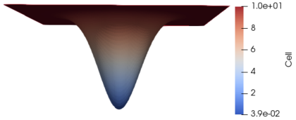
(a) Initial cell density $u_{0}$

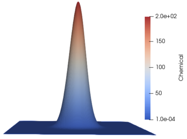
(b) Initial chemical concentration $v_{0}$

Figure 1: Initial conditions.

In the case of the scheme US, it can be observed that $u_{h}$ is negative for some $\boldsymbol{x}\in\Omega$ in some times $t_{n}>0$, but when $h\rightarrow 0$ these values are closer to $0$; while in the case of the scheme LC, when $h\rightarrow 0$ very negative cell densities $u_{h}$ are obtained for some $\boldsymbol{x}\in\Omega$ in some times $t_{n}>0$ (see Figure 2(a)-(c)). On the other hand, the same behavior is observed for the minimum of $v_{h}$ in both schemes. In fact, independently of $h$, if $v_{0}$ is positive, then $v_{h}$ is also positive (we show this behavior in Figure 2(d) for the case $h=\frac{1}{35}$, but the same holds for the cases $h=\frac{1}{75},\frac{1}{150}$).

6.2 Unconditional Stability

In this subsection, the stability with respect to the energies $\mathcal{E}(u,v)$ and $\mathcal{E}(u,{\boldsymbol{\sigma}})$, given in (25) and (33) respectively, are numerically compared. Following line by line the proof of Lemma 4.7, the unconditional energy-stability with respect to $\mathcal{E}(u,{\boldsymbol{\sigma}})$ for the fully discrete schemes corresponding to schemes US and LC can be deduced. In fact, if $(u_{n},{\boldsymbol{\sigma}}_{n})$ is any solution of the fully discrete schemes associated to US or LC, the following relation holds

$$RE(u_{n},{\boldsymbol{\sigma}}_{n}):=\delta_{t}\mathcal{E}(u_{n},{\boldsymbol{\sigma}}_{n})+\|\nabla u_{n}\|_{0}^{2}+\displaystyle\frac{1}{2}\|{\boldsymbol{\sigma}}_{n}\|_{1}^{2}\leq 0,\ \ \forall n.$$ (102)

However, considering the “exact” energy $\mathcal{E}(u,v)$ given in (25), in the case of fully discrete schemes, it is not clear how to prove unconditional energy-stability of schemes US, LC and UV with respect to this energy. Therefore, it is interesting to study the behaviour of the corresponding residual

$$RE(u_{n},v_{n}):=\delta_{t}\mathcal{E}(u_{n},v_{n})+\|\nabla u_{n}\|_{0}^{2}+\displaystyle\frac{1}{2}\|\Delta_{h}v_{n}\|_{0}^{2}+\frac{1}{2}\|\nabla v_{n}\|_{0}^{2}.$$

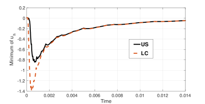
(a) Minimum values of $u_{h}$, with $h=\frac{1}{35}$

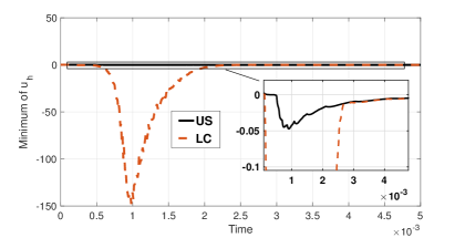
(b) Minimum values of $u_{h}$, with $h=\frac{1}{75}$

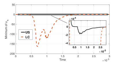
(c) Minimum values of $u_{h}$, with $h=\frac{1}{150}$

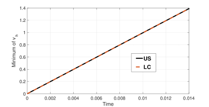
(d) Minimum values of $v_{h}$, with $h=\frac{1}{35}$

Figure 2: Minimum of $u_{h}$ and $v_{h}$ computed by using the schemes US and LC with different values of $h$.

With this aim, we take $k=10^{-5}$ (in order to minimize the influence of the numerical dissipation terms $\frac{k}{2}\|\delta_{t}u_{n}\|_{0}^{2}$ and $\frac{k}{4}\|\delta_{t}{\boldsymbol{\sigma}}_{n}\|_{0}^{2}$), $h=\frac{1}{25}$ and the initial conditions

$$u_{0}=-10xy\,(2-x)(2-y)\exp(-10(y-1)^{2}-10(x-1)^{2})+10.0001$$

$$v_{0}=20xy\,(2-x)(2-y)\exp(-30(y-1)^{2}-30(x-1)^{2})+0.0001.$$

We obtain that:

1. The schemes US and LC satisfy the energy decreasing in time property (54) for the modified energy $\mathcal{E}(u,{\boldsymbol{\sigma}})$, see Figure 3(a).

2. The schemes US and LC satisfy (102), see Figure 3(b).

3. The schemes US, LC and UV satisfy the energy decreasing in time property for the exact energy $\mathcal{E}(u,v)$, that is, $\mathcal{E}(u_{n},v_{n})\leq\mathcal{E}(u_{n-1},v_{n-1})$ for all $n$, see Figure 3(c).

4. The schemes US, LC and UV have $RE(u_{n},v_{n})>0$ for some $t_{n}\geq 0$. However, it is observed that the residual $RE(u_{n},v_{n})$ in the schemes US and LC is much smaller than the residual of the scheme UV, see Figure 3(d).

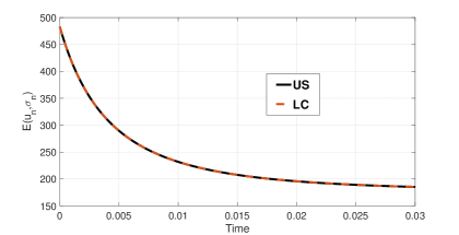
(a) $\mathcal{E}(u_{n},{\boldsymbol{\sigma}}_{n})$ in the schemes US and LC

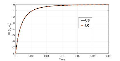
(b) $RE(u_{n},{\boldsymbol{\sigma}}_{n})$ in the schemes US and LC

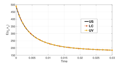
(c) $\mathcal{E}(u_{n},v_{n})$ in the schemes US, LC and UV

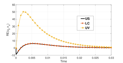
(d) $RE(u_{n},v_{n})$ in the schemes US, LC and UV.

Figure 3: Energy-stability of the schemes US, LC and UV for both energies $\mathcal{E}(u_{n},{\boldsymbol{\sigma}}_{n})$ and $\mathcal{E}(u_{n},v_{n})$.

Appendix A
In order to prove the solvability of (51), we will use the Leray-Schauder fixed point theorem. With this aim, we define the operator $R:L^{4}(\Omega)\times\boldsymbol{L}^{4}(\Omega)\rightarrow L^{4}(\Omega)\times\boldsymbol{L}^{4}(\Omega)$ by $R(\widetilde{u},\widetilde{\boldsymbol{\sigma}})=(u,{\boldsymbol{\sigma}})$, such that $(u,{\boldsymbol{\sigma}})$ solves the following linear decoupled problems

$$\begin{array}[c]{lll}\displaystyle\frac{1}{k}(u,\overline{u})+(\nabla u,\nabla\overline{u})=\displaystyle\frac{1}{k}(u_{n-1},\overline{u})-(\widetilde{u}_{+}\widetilde{\boldsymbol{\sigma}},\nabla\overline{u}),\ \ \forall\overline{u}\in{H}^{1}(\Omega),\vspace{0,2 cm}\\ \displaystyle\frac{1}{k}({\boldsymbol{\sigma}},\overline{\boldsymbol{\sigma}})+\langle B{\boldsymbol{\sigma}},\overline{\boldsymbol{\sigma}}\rangle=\displaystyle\frac{1}{k}({\boldsymbol{\sigma}}_{n-1},\overline{\boldsymbol{\sigma}})-(\widetilde{u}^{2},\nabla\cdot\overline{\boldsymbol{\sigma}}),\ \ \forall\overline{\boldsymbol{\sigma}}\in\boldsymbol{H}^{1}_{\sigma}(\Omega).\end{array}$$ (103)

1. $R$ is well defined. Let $(\widetilde{u},\widetilde{\boldsymbol{\sigma}})\in L^{4}(\Omega)\times\mathbf{L}^{4}(\Omega)$ and consider the following bilinear forms $\widetilde{a}:{H}^{1}(\Omega)\times{H}^{1}(\Omega)\rightarrow\mathbb{R}$, $\widetilde{b}:\boldsymbol{H}^{1}_{\sigma}(\Omega)\times\boldsymbol{H}^{1}_{\sigma}(\Omega)\rightarrow\mathbb{R}$, and the linear forms $l_{1}:{H}^{1}(\Omega)\rightarrow\mathbb{R}$ and $l_{2}:\boldsymbol{H}^{1}_{\sigma}(\Omega)\rightarrow\mathbb{R}$ given by

   $$\widetilde{a}(u,\overline{u})=\displaystyle\frac{1}{k}(u,\overline{u})+(\nabla u,\nabla\overline{u}),\quad\widetilde{b}({\boldsymbol{\sigma}},\overline{{\boldsymbol{\sigma}}})=\displaystyle\frac{1}{k}({\boldsymbol{\sigma}},\overline{{\boldsymbol{\sigma}}})+\langle B{\boldsymbol{\sigma}},\overline{\boldsymbol{\sigma}}\rangle,$$

   $$l_{1}(\overline{u})=\frac{1}{k}\int_{\Omega}u_{n-1}\overline{u}-\int_{\Omega}\widetilde{u}_{+}\widetilde{\boldsymbol{\sigma}}\cdot\nabla\bar{u},\quad l_{2}(\overline{{\boldsymbol{\sigma}}})=\frac{1}{k}\int_{\Omega}{\boldsymbol{\sigma}}_{n-1}\overline{{\boldsymbol{\sigma}}}-\int_{\Omega}\widetilde{u}^{2}\nabla\cdot\overline{{\boldsymbol{\sigma}}},$$

   for all $u,\overline{u}\in{H}^{1}(\Omega)$ and ${\boldsymbol{\sigma}},\overline{{\boldsymbol{\sigma}}}\in\boldsymbol{H}^{1}_{\sigma}(\Omega)$. Then, using the Hölder inequality and Sobolev embeddings, we can verify that $\widetilde{a}$ and $\widetilde{b}$ are continuous and coercive on ${H}^{1}(\Omega)$ and $\boldsymbol{H}^{1}_{\sigma}(\Omega)$ respectively, and $l_{1}\in{H}^{1}(\Omega)^{\prime}$ and $l_{2}\in\boldsymbol{H}^{1}_{\sigma}(\Omega)^{\prime}$. Thus, from Lax-Milgram theorem, there exists a unique $(u,{\boldsymbol{\sigma}})\in H^{1}(\Omega)\times\boldsymbol{H}^{1}_{\sigma}(\Omega)\hookrightarrow L^{4}(\Omega)\times\boldsymbol{L}^{4}(\Omega)$ solution of (103).

2. Now, let us prove that all possible fixed points of $\lambda R$ (with $\lambda\in(0,1]$) are bounded. In fact, observe that if $(u,{\boldsymbol{\sigma}})$ is a fixed point of $\lambda R$, then $(u,{\boldsymbol{\sigma}})$ satisfies the coupled problem

   $$\left\{\begin{array}[c]{lll}\displaystyle\widetilde{a}(u,\overline{u})=\displaystyle\frac{\lambda}{k}(u_{n-1},\overline{u})-\lambda(u_{+}{\boldsymbol{\sigma}},\nabla\overline{u}),\ \ \forall\overline{u}\in{H}^{1}(\Omega),\vspace{0,2 cm}\\ \displaystyle\widetilde{b}({\boldsymbol{\sigma}},\overline{\boldsymbol{\sigma}})=\displaystyle\frac{\lambda}{k}({\boldsymbol{\sigma}}_{n-1},\overline{\boldsymbol{\sigma}})-\lambda(u^{2},\nabla\cdot\overline{\boldsymbol{\sigma}}),\ \ \forall\overline{\boldsymbol{\sigma}}\in\boldsymbol{H}^{1}_{\sigma}(\Omega),\end{array}\right.$$ (104)

   (because $\lambda R(u,{\boldsymbol{\sigma}})=(u,{\boldsymbol{\sigma}})$ implies $R(u,{\boldsymbol{\sigma}})=(\frac{1}{\lambda}u,\frac{1}{\lambda}{\boldsymbol{\sigma}})$). Proceeding as in Part A of the proof of Theorem 4.4, it can be proved that if $(u,{\boldsymbol{\sigma}})$ is a solution of (104), then $u\geq 0$, which implies that $u=u_{+}$. Then, testing by $\overline{u}=u$ and $\overline{\boldsymbol{\sigma}}=\frac{1}{2}{\boldsymbol{\sigma}}$ in (104)₁ and (104)₂, and taking into account that $\lambda\in(0,1]$, one obtains

   $$\frac{1}{4}\|(u,{\boldsymbol{\sigma}})\|_{0}^{2}+\displaystyle\frac{k}{2}\|(\nabla u,{\boldsymbol{\sigma}})\|_{L^{2}\times H^{1}}^{2}\leq\displaystyle C\lambda^{2}\|(u_{n-1},{\boldsymbol{\sigma}}_{n-1})\|_{0}^{2}\leq C(u_{n-1},{\boldsymbol{\sigma}}_{n-1}).$$

   Thus, we deduce that $\|(u,{\boldsymbol{\sigma}})\|_{L^{4}}\leq C\|(u,{\boldsymbol{\sigma}})\|_{1}\leq C(u_{n-1},{\boldsymbol{\sigma}}_{n-1})$.

3. We prove that $R$ is continuous. Let $\{(\widetilde{u}^{l},\widetilde{\boldsymbol{\sigma}}^{l})\}_{l\in\mathbb{N}}\subset{L}^{4}(\Omega)\times\boldsymbol{L}^{4}(\Omega)$ be a sequence such that

   $$(\widetilde{u}^{l},\widetilde{\boldsymbol{\sigma}}^{l})\rightarrow(\widetilde{u},\widetilde{\boldsymbol{\sigma}})\ \mbox{ in }{L}^{4}(\Omega)\times\mathbf{L}^{4}(\Omega),\quad\hbox{as $l\to+\infty$}.$$ (105)

   Therefore, $\{(\widetilde{u}^{l},\widetilde{\boldsymbol{\sigma}}^{l})\}_{l\in\mathbb{N}}$ is bounded in ${L}^{4}(\Omega)\times\mathbf{L}^{4}(\Omega)$, and from item 1 we deduce that $\{(u^{l},\boldsymbol{\sigma}^{l})=R(\widetilde{u}^{l},\widetilde{\boldsymbol{\sigma}}^{l})\}_{l\in\mathbb{N}}$ is bounded in ${H}^{1}(\Omega)\times\boldsymbol{H}^{1}(\Omega)$. Then, there exists a subsequence $\{R(\widetilde{u}^{l^{r}},\widetilde{\boldsymbol{\sigma}}^{l^{r}})\}_{r\in\mathbb{N}}$ such that

   $$R(\widetilde{u}^{l^{r}},\widetilde{\boldsymbol{\sigma}}^{l^{r}})\rightarrow(u^{\prime},{\boldsymbol{\sigma}}^{\prime})\ \ \mbox{ weakly in }H^{1}(\Omega)\times\boldsymbol{H}^{1}(\Omega)\ \mbox{ and strongly in }L^{4}(\Omega)\times\boldsymbol{L}^{4}(\Omega).$$ (106)

   Thus, from (105)-(106), a standard pass to the limit as $r\to+\infty$ in (103), allows to deduce that $R(\widetilde{u},\widetilde{\boldsymbol{\sigma}})=({u}^{\prime},{\boldsymbol{\sigma}}^{\prime})$. Therefore, any convergent subsequence of $\{R(\widetilde{u}^{l},\widetilde{\boldsymbol{\sigma}}^{l})\}_{l\in\mathbb{N}}$ converges to $R(\widetilde{u},\widetilde{\boldsymbol{\sigma}})$ strongly in $L^{4}(\Omega)\times\boldsymbol{L}^{4}(\Omega)$. From uniqueness of $R(\widetilde{u},\widetilde{\boldsymbol{\sigma}})$, one concludes that $R(\widetilde{u}^{l},\widetilde{\boldsymbol{\sigma}}^{l})\rightarrow R(\widetilde{u},\widetilde{\boldsymbol{\sigma}})$ in $L^{4}(\Omega)\times\boldsymbol{L}^{4}(\Omega)$. Thus, $R$ is continuous.

4. $R$ is compact. In fact, if $\{(\widetilde{u}^{l},\widetilde{\boldsymbol{\sigma}}^{l})\}_{l\in\mathbb{N}}$ is a bounded sequence in ${L}^{4}(\Omega)\times\boldsymbol{L}^{4}(\Omega)$ and we denote $(u^{l},\boldsymbol{\sigma}^{l})=R(\widetilde{u}^{l},\widetilde{\boldsymbol{\sigma}}^{l})$, then we can deduce

   $$\frac{1}{2k}\|(u^{l},{\boldsymbol{\sigma}^{l}})\|_{0}^{2}+\frac{1}{2}\|(\nabla u^{l},{\boldsymbol{\sigma}}^{l})\|_{L^{2}\times H^{1}}^{2}\leq\displaystyle\frac{1}{2k}\|(u_{n-1},{\boldsymbol{\sigma}}_{n-1})\|_{0}^{2}+\frac{1}{2}\|\widetilde{u}^{l}\|_{L^{4}}^{2}\|\widetilde{\boldsymbol{\sigma}}^{l}\|_{L^{4}}^{2}+\frac{1}{2}\|\widetilde{u}^{l}\|_{L^{4}}^{4}\leq C,$$

   where $C$ is independent of $l\in\mathbb{N}$. Therefore, we conclude that $\{R(\widetilde{u}^{l},\widetilde{\boldsymbol{\sigma}}^{l})\}_{l\in\mathbb{N}}$ is bounded in ${H}^{1}(\Omega)\times\boldsymbol{H}^{1}(\Omega)$ which is compactly embedded in ${L}^{4}(\Omega)\times\boldsymbol{L}^{4}(\Omega)$, and thus $R$ is compact.

The hypotheses of the Leray-Schauder fixed point theorem are then satisfied, and the existence of a fixed point for the map $R$ is proved. This fixed point $R(u,{\boldsymbol{\sigma}})=(u,{\boldsymbol{\sigma}})$ is a solution of (51).

References

• [1] C. Amrouche and N.E.H. Seloula, $L^{p}$-theory for vector potentials and Sobolev’s inequalities for vector fields: application to the Stokes equations with pressure boundary conditions. Math. Models Methods Appl. Sci. 23 (2013), no. 1, 37–92.
• [2] G. Chamoun, M. Saad and R. Talhouk, Monotone combined edge finite volume-finite element scheme for anisotropic Keller-Segel model. Numer. Methods Partial Differential Equations 30 (2014), no. 3, 1030–1065.
• [3] T. Cieslak, P. Laurencot and C. Morales-Rodrigo, Global existence and convergence to steady states in a chemorepulsion system. Parabolic and Navier-Stokes equations. Part 1, 105-117, Banach Center Publ., 81, Part 1, Polish Acad. Sci. Inst. Math., Warsaw, 2008.
• [4] P. De Leenheer, J. Gopalakrishnan and E. Zuhr, Nonnegativity of exact and numerical solutions of some chemotactic models. Comput. Math. Appl. 66 (2013), no. 3, 356–375.
• [5] F. Demengel and G. Demengel, Functional spaces for the theory of elliptic partial differential equations. Universitext. Springer, London; EDP Sciences, Les Ulis (2012).
• [6] Y. Epshteyn and A. Izmirlioglu, Fully discrete analysis of a discontinuous finite element method for the Keller-Segel chemotaxis model. J. Sci. Comput. 40 (2009), no. 1-3, 211–256.
• [7] E. Feireisl and A. Novotný, Singular limits in thermodynamics of viscous fluids. Advances in Mathematical Fluid Mechanics. Birkhäuser Verlag, Basel (2009).
• [8] F. Filbet, A finite volume scheme for the Patlak-Keller-Segel chemotaxis model. Numer. Math. 104 (2006), no. 4, 457–488.
• [9] F. Guillén-González, M.A. Rodríguez-Bellido and D.A. Rueda-Gómez, Study of a chemo-repulsion model with quadratic production. Part II: Analysis of an unconditional energy-stable fully discrete scheme. (Submitted).
• [10] F. Guillén-González, M.A. Rodríguez-Bellido and D.A. Rueda-Gómez, Unconditionally energy stable fully discrete schemes for a chemo-repulsion model. Math. Comp. 88 (2019), no. 319, 2069–2099.
• [11] J.G. Heywood and R. Rannacher, Finite element approximation of the nonstationary Navier-Stokes problem. IV. Error analysis for second order time discretization. SIAM J. Numer. Anal. 27 (1990), 353–384.
• [12] J.L. Lions, Quelques méthodes de résolution des problèmes aux limites non linéaires. (French) Dunod; Gauthier-Villars, Paris (1969).
• [13] M. Marion and R. Temam, Navier-Stokes equations: theory and approximation. Handbook of numerical analysis, Vol. VI, 503–688, Handb. Numer. Anal., VI, North-Holland, Amsterdam (1998).
• [14] A. Marrocco, Numerical simulation of chemotactic bacteria aggregation via mixed finite elements. M2AN Math. Model. Numer. Anal. 37 (2003), no. 4, 617–630.
• [15] J. Necas, Les Méthodes Directes en Théorie des Equations Elliptiques. Ed. Academia, Prague (1967).
• [16] N. Saito, Conservative upwind finite-element method for a simplified Keller-Segel system modelling chemotaxis. IMA J. Numer. Anal. 27 (2007), no. 2, 332–365.
• [17] N. Saito, Error analysis of a conservative finite-element approximation for the Keller-Segel system of chemotaxis. Commun. Pure Appl. Anal. 11 (2012), no. 1, 339–364.
• [18] J. Shen, Long time stability and convergence for fully discrete nonlinear Galerkin methods. Appl. Anal. 38 (1990), 201–229.
• [19] R. Temam, Infinite-dimensional dynamical systems in mechanics and physics. Second edition. Applied Mathematical Sciences, 68. Springer-Verlag, New York (1997).
• [20] M. Winkler, A critical blow-up exponent in a chemotaxis system with nonlinear signal production. Nonlinearity 31 (2018), no. 5, 2031–2056.
• [21] J. Zhang, J. Zhu and R. Zhang, Characteristic splitting mixed finite element analysis of Keller-Segel chemotaxis models. Appl. Math. Comput. 278 (2016), 33–44.