Linearized Flux Evolution (LiFE): A Technique for Rapidly Adapting Fluxes from Full-Physics Radiative Transfer Models

Abstract

Solar and thermal radiation are critical aspects of planetary climate, with gradients in radiative energy fluxes driving heating and cooling. Climate models require that radiative transfer tools be versatile, computationally efficient, and accurate. Here, we describe a technique that uses an accurate full-physics radiative transfer model to generate a set of atmospheric radiative quantities which can be used to linearly adapt radiative flux profiles to changes in the atmospheric and surface state—the Linearized Flux Evolution (LiFE) approach. These radiative quantities describe how each model layer in a plane-parallel atmosphere reflects and transmits light, as well as how the layer generates diffuse radiation by thermal emission and by scattering light from the direct solar beam. By computing derivatives of these layer radiative properties with respect to dynamic elements of the atmospheric state, we can then efficiently adapt the flux profiles computed by the full-physics model to new atmospheric states. We validate the LiFE approach, and then apply this approach to Mars, Earth, and Venus, demonstrating the information contained in the layer radiative properties and their derivatives, as well as how the LiFE approach can be used to determine the thermal structure of radiative and radiative-convective equilibrium states in one-dimensional atmospheric models.

1 Introduction

Plane-parallel, horizontally homogenous radiative transfer calculations are the standard approach to exploring solar and thermal radiation fields in Earth and planetary atmospheres. In the context of planetary climate models, which derive an equilibrium or quasi-equilibrium surface-atmosphere state from a specified set of initial conditions, it is the role of a radiative transfer model to compute the state-dependent vertical net radiative energy flux. Gradients in the net radiative flux contribute to atmospheric heating or cooling, which the climate model uses to update the surface and atmospheric state [1, 2, 3, 4]. Since the net radiative flux is a function of these state properties, the radiative transfer model must then re-compute the radiative fluxes for any new atmospheric state. This modeling approach demands that the radiative transfer model be both accurate and computationally efficient [e.g., 5, 6].

While a number of techniques have been developed to accurately compute radiative energy fluxes in a realistic, vertically-inhomogeneous planetary atmosphere where gases and airborne particles contribute to the absorption, emission, and multiple scattering of solar or thermal radiation [7, 8, 9], these approaches are typically too computationally expensive to be used within a general climate model, which requires fluxes to be computed and integrated over a large range of wavelengths (or frequencies). Thus, climate models tend to rely on parametrized radiative transfer tools [10, 11, 12, 13, 14, 15, 16, 17]. However, the tuning and parameterizations used in these tools can lead to errors and biases in predictions when the model is used to study conditions for which it was not designed.

Here, we describe a technique for efficiently adapting radiative fluxes, computed with a full-physics radiative transfer model, to changes in the atmospheric state—the LiFE approach. This technique combines linear “flux Jacobians” with an approximate method motivated by two-stream adding methods [18, 19, 20] to adapt the radiation field to changes in the atmospheric and surface thermal structure and optical properties as they evolve. Thus, the LiFE approach is applicable to a wide range of problems in planetary climate.

In what follows, we begin with a description of the LiFE approach (Section 2), including a discussion of how we compute the requisite layer radiative properties and the flux Jacobians associated with each property (Sections 2.2 and 2.3, respectively). We then present a validation of the LiFE approach in Section 3. Next we demonstrate a sequence of example applications of the LiFE approach (Section 4), which focus on Mars (Section 4.1), Earth (Section 4.2), and Venus (Section 4.3). For a simple test case, Section 5 shows a comparison of a LiFE-derived atmospheric thermal profile to an atmospheric state computed using a widely-adopted, one-dimensional radiative-convective planetary climate model. Note that the Appendix contains an intuitive example calculation using the approximate two-stream flux adding technique, and, for completeness, clear derivations of the flux adding relationships adopted for this application.

2 Description of LiFE Approach

The Linearized Flux Evolution (LiFE) approach pairs a full-physics radiative transfer model with flux Jacobians and an approximate method motivated by two-stream flux adding techniques [18, 19, 20] to rapidly adapt radiative flux profiles in plane-parallel planetary atmospheres to changes in atmospheric state. Given an initial atmospheric and surface state, the full-physics model is used to compute the upwelling and downwelling radiative energy fluxes at the boundaries between model atmospheric layers. Additionally, for each atmospheric layer, the full-physics model computes a set of frequency-dependent layer radiative properties and their flux Jacobians, which are used to determine the first derivative of the upward and downward solar and thermal fluxes at each layer boundary with respect to changes in the atmospheric or surface thermal structure or optical properties.

In the LiFE approach, we decompose a vertically inhomogeneous, non-isothermal atmosphere into a series of discrete interacting layers. Each layer is characterized by an effective flux reflectivity, transmissivity, and upwelling and downwelling “source terms” (collectively referred to as “layer radiative properties”). While adding approaches are most correctly applied to radiances [21, Chapter VII], we specifically construct these layer radiative properties to reproduce the level-dependent fluxes from a full-physics model when used within our flux adding method. The accuracy of the computed Jacobians for the layer radiative properties (and, thus, the accuracy of the flux adding approach) decays as the atmosphere and surface evolve from their initial state, eventually requiring a recalculation of the flux field and layer Jacobians using the full-physics model.

Unlike analytic two-stream adding methods [e.g., 19], the layer radiative properties used here are not derived from analytic two-stream solutions to the equation of transfer. Instead, these properties are defined such that the two-stream adding method exactly reproduces the flux distributions generated by the full-physics model for a specified atmospheric state. Similarly, the reflectivity, transmissivity, and source term Jacobians are defined to approximate the linear response of the fluxes in the full-physics model to small perturbations in the layer optical properties (e.g., differential optical depth, single scattering albedo, scattering phase function) associated with changes in temperature, or trace gas and aerosol profiles.

In general, bolometric or band-integrated radiances and fluxes have a non-linear dependence on the atmospheric thermal structure and optical properties. However, by applying a linear flux correction over monochromatic (or near-monochromatic) spectral intervals (i.e., of order 1–10 cm^-1), we aim to minimize sensitivity within the LiFE approach to the non-linear effects that arise in wavelength-integrated quantities. Our linear flux correction approach was motivated by atmospheric retrieval algorithms. Within a retrieval framework [22], a synthetic spectrum and associated linear radiance Jacobians are generated for an assumed atmospheric and surface state. These results are then used within the context of a non-linear least-squares fitting algorithm to produce a better fit to an observed spectrum. Here, like in the LiFE approach, the non-linear relationship between radiances (or fluxes) and optical properties is approximated as quasi-linear for small perturbations to the atmospheric and surface state.

In the following sub-sections, we first present the flux adding technique, which will introduce the layer radiative properties relevant to LiFE. We then discuss how we use a full-physics radiative transfer model to compute the layer radiative properties. Finally, we discuss how we compute the Jacobians and how these are used to rapidly adapt radiative flux profiles as an atmospheric state evolves from its initial conditions toward an equilibrium state. While these discussions typically apply to a narrow spectral range within a spectrally resolved model, an intuitive example of the LiFE approach which uses gray radiative transfer is provided in the Appendix to help the reader better understand the technique.

2.1 Flux Adding

The flux adding technique relates the diffuse upwelling and downwelling radiative energy fluxes, defined at the boundaries between a collection of homogenous atmospheric layers, to the radiative properties of each of these layers [23, 20, 24]. By stacking homogenous layers to create inhomogeneous layers, we can recursively relate the radiative fluxes to the properties of successively thicker atmospheric layers, eventually determining the fluxes at all required levels throughout the atmosphere. This process is analogous to previous two-stream adding techniques [18, 19, 20].

Each homogenous layer in a model atmosphere is assigned a reflectivity and transmissivity, which describe how the layer reflects and transmits diffuse incident flux. Additionally, each layer can add radiation to the diffuse flux field, either by scattering light from a direct solar beam, or by emitting thermal radiation. A layer’s ability to add diffuse flux is described by layer source terms, which are not necessarily identical for contributions to the upwelling and downwelling diffuse flux fields. The frequency-dependent diffuse flux reflectivity, transmissivity, and upwelling and downwelling source terms for layer $j$ will be labeled $r_{j}$, $t_{j}$, $s^{+}_{j}$, and $s^{-}_{j}$, respectively. The diffuse flux emerging from layer $j$, $F^{+}_{j-1}$ and $F^{-}_{j}$, is related to the incident diffuse flux, $F^{-}_{j-1}$ and $F^{+}_{j}$, through

$$F^{+}_{j-1}=r_{j}F^{-}_{j-1}+t_{j}F^{+}_{j}+s^{+}_{j}\ ,$$ (1)

$$F^{-}_{j}=t_{j}F^{-}_{j-1}+r_{j}F^{+}_{j}+s^{-}_{j}\ .$$ (2)

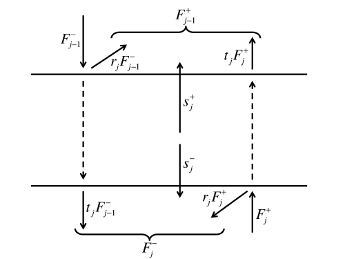
Figure 1: Schematic of layer radiative properties: the diffuse flux reflectivity ($r_{j}$), transmissivity ($t_{j}$), and the layer source terms, $s^{+}_{j}$ and $s^{-}_{j}$. The fluxes ($F$) are defined at the layer boundaries, and are either upwelling ($+$) or downwelling ($-$). All terms are frequency-dependent.

Figure 1 shows a schematic of these layer properties and fluxes.

As is derived in the Appendix, two homogenous layers with different radiative properties can be combined to yield an inhomogeneous layer. The radiative properties of subsequently thicker inhomogeneous layers can be obtained by adding homogenous layers to either the bottom or top of an inhomogeneous layer. These downward and upward adding procedures produce a recursive set of relations that describe how the inhomogeneous layers reflect and generate diffuse flux.

When adding downwards, homogenous layer $j$ is added to the base of an inhomogeneous layer that extends from the top of the atmosphere ($j=0$) to layer $j-1$. We define the inhomogeneous layer reflectivity and source term for adding downward, $R^{-}_{0,j-1}$ and $S^{-}_{0,j-1}$, respectively, and have

$$F^{-}_{j-1}=R^{-}_{0,j-1}F^{+}_{j-1}+S^{-}_{0,j-1}\ ,$$ (3)

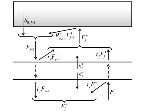
Figure 2: Schematic diagram of combining a homogenous and in homogenous layer by adding the former to the top of the latter. The inhomogeneous layer generates diffuse downwelling flux through a source term, $S^{-}_{0,j-1}$, and reflects diffuse upwelling flux downward through a reflectivity term, $R^{-}_{0,j-1}$. Other symbols are as in Figure 1.

which are generally frequency-dependent, and are schematically shown in Figure 2. The reflectivity and source term for the newly-extended inhomogeneous layer are then given by (see Appendix)

$$R^{-}_{0,j}=r_{j}+\frac{t_{j}^{2}R^{-}_{0,j-1}}{1-r_{j}R^{-}_{0,j-1}}\ ,$$ (4)

and

$$S^{-}_{0,j}=s^{-}_{j}+\frac{t_{j}\left(S^{-}_{0,j-1}+s^{+}_{j}R^{-}_{0,j-1}\right)}{1-r_{j}R^{-}_{0,j-1}}\ .$$ (5)

Similarly, in upwards adding, homogenous layer $j$ is added to the top of an inhomogeneous layer extending from the base of the atmosphere $j=N-1$ to the bottom of layer $j$. For this scenario, we have

$$F_{j}^{+}=R_{j+1,N}^{+}F_{j}^{-}+S_{j+1,N}^{+}$$ (6)

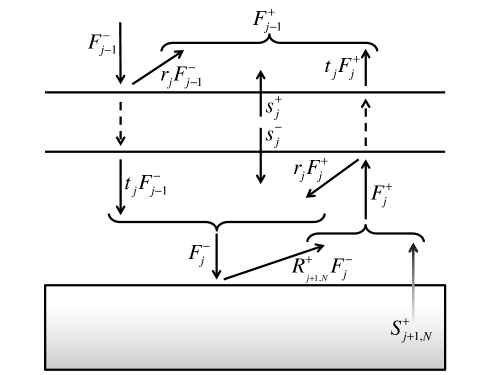
Figure 3: Schematic diagram of combining a homogenous and in homogenous layer by adding the former to the bottom of the latter. The inhomogeneous layer generates diffuse upwelling flux through a source term, $S^{+}_{j+1,N}$, and reflects diffuse downwelling flux upward through a reflectivity term, $R^{+}_{j+1,N}$. Other symbols are as in Figure 1.

where we have defined the inhomogeneous layer reflectivity and source term for adding upward as $R_{j+1,N}^{+}$ and $S_{j+1,N}^{+}$, respectively. Figure 3 shows a schematic of the process of adding a homogenous layer to the base of an inhomogeneous layer. The recursive relations for upward adding are then given by (see Appendix)

$$R_{j,N}^{+}=r_{j}+\frac{t_{j}^{2}R^{+}_{j+1,N}}{1-r_{j}R^{+}_{j+1,N}}\ ,$$ (7)

and

$$S_{j,N}^{+}=s^{+}_{j}+\frac{t_{j}\left(S^{+}_{j+1,N}+s^{-}_{j}R^{+}_{j+1,N}\right)}{1-r_{j}R^{+}_{j+1,N}}\ .$$ (8)

Note that a convenient expression can be found by inserting the equivalent expression to Equation 3 for an inhomogeneous layer extending down to layer $j$ into Equation 6. After simplifying, this gives us

$$F_{j}^{+}=\frac{S^{+}_{j+1,N}+R_{j+1,N}^{+}S^{-}_{1,j}}{1-R_{j+1,N}^{+}R_{1,j}^{-}}\ .$$ (9)

This relation provides the upwelling flux at each model level in terms of quantities that can be recursively determined from only the homogenous layer radiative properties. The equivalent expression for downwelling flux is determined via a similar insertion, and is given by

$$F_{j-1}^{-}=\frac{S^{-}_{0,j-1}+R_{0,j-1}^{-}S^{+}_{j,N}}{1-R_{0,j-1}^{-}R_{j,N}^{+}}\ .$$ (10)

The relations described above allow us to compute the upwelling and downwelling fluxes at each model level (i.e., at the boundaries between homogenous atmospheric layers) when given the radiative properties for each homogenous model atmospheric layer. Top- and bottom-of-atmosphere boundary conditions must also be provided. Here, we adopt the same boundary conditions that are used by the full-physics model: (1) the reflectivity of “space" is zero (i.e., $r_{0}=R^{-}_{0,0}=0$), (2) the top-of-atmosphere downwelling flux is known ($F^{-}_{0}=s^{-}_{0}=S^{-}_{0,0}$), (3) a frequency-dependent surface albedo is known ($A_{\nu}$, with $r_{N}=R^{+}_{N,N}=A_{\nu}$), and (4) a bottom-of-atmosphere upwelling flux is set [e.g., $s^{+}_{N}=S^{+}_{N,N}=A_{\nu}S^{-}_{0,N}+(1-A_{\nu})\pi B_{\nu}(T_{s})$, where the first term on the right-hand side represents reflected downwelling radiation and the second term represents surface emission via a Planck function at the surface temperature, $T_{s}$, multiplied by the surface emissivity, which is $1-A_{\nu}$ by Kirchoff’s Law]. The steps required in computing $F^{+}_{j}$ and $F^{-}_{j}$ within a particular spectral interval and for all values of $j$ are then:

1. use the top-of-atmosphere boundary conditions, $R^{-}_{0,0}=0$ and $S^{-}_{0,0}=F^{-}_{0}$, to recursively add layers downward, using Equations 4 and 5 to solve for $R^{-}_{0,j}$ and $S^{-}_{0,j}$ for all values of $j$;

2. use the bottom-of-atmosphere boundary conditions, $R^{+}_{N,N}=A_{\lambda}$, and $S^{+}_{N,N}=A_{\lambda}S^{-}_{0,N}$ or $S^{+}_{N,N}=(1-A_{\lambda})\pi B_{\lambda}(T_{s})$, to recursively add layers upward, using Equations 7 and 8 to solve for $R^{+}_{j,N}$ and $S^{+}_{j,N}$ for all values of $j$;

3. use the computed sets of inhomogeneous layer radiative properties to compute the upwelling flux at each model level using Equation 9;

4. use the upwelling fluxes and the inhomogeneous layer radiative properties to compute the downwelling fluxes at each model level using Equation 3.

2.2 Determining Homogenous Layer Radiative Properties

A full-physics radiative transfer model (e.g., a multiple scattering, spectrum resolving [line-by-line], multi-stream radiative transfer model) is used to compile the optical properties of the surface and atmosphere at the beginning of each experiment. It then derives the angle-dependent radiances and fluxes throughout the atmospheric column. The full-physics model is then used to obtain the layer reflectivity, transmissivity, and source terms. These properties and fluxes are defined on a spectral grid that is fine enough to resolve all of the frequency-dependent changes in the atmospheric or surface optical properties.

Given an the atmospheric state, $\boldsymbol{x}$, the full-physics model solves the one-dimensional, plane-parallel radiative transfer equation at frequency $\nu$ in an inhomogeneous scattering, absorbing, and emitting atmosphere, which is given by

$$\mu\frac{dI_{\nu}}{d\tau_{\nu}}=I_{\nu}\left(\tau_{\nu},\mu,\phi,\boldsymbol{x}\right)-S_{\nu}\left(\tau_{\nu},\mu,\phi,\boldsymbol{x}\right)\ ,$$ (11)

where $I_{\nu}$ is the spectral radiance, $\tau_{\nu}=\tau_{\nu}\left(\boldsymbol{x}\right)$ is the frequency-dependent extinction optical depth (which increases towards higher pressures), $\mu$ is the cosine of the zenith angle, and $\phi$ is the azimuth angle. The source function, $S_{\nu}$, is given by

$$\begin{array}[]{ll}S_{\nu}\left(\tau_{\nu},\mu,\phi,\boldsymbol{x}\right)=&\omega_{\nu}F^{\odot}_{\nu}e^{-\tau_{\nu}/\mu_{\odot}}\cdot P_{\nu}\left(\tau_{\nu},\mu,\phi,-\mu_{\odot},\phi_{\odot},\boldsymbol{x}\right)/4\pi\\ &+\left(1-\omega_{\nu}\right)B_{\nu}\left(T\left(\tau_{\nu}\right)\right)\\ &+\omega_{\nu}\int_{0}^{2\pi}d\phi^{\prime}\int_{-1}^{1}d\mu^{\prime}\cdot I_{\nu}\left(\tau_{\nu},\mu^{\prime},\phi^{\prime},\boldsymbol{x}\right)P_{\nu}\left(\tau_{\nu},\mu,\phi,\mu^{\prime},\phi^{\prime},\boldsymbol{x}\right)/4\pi\ ,\end{array}$$ (12)

where $\omega_{\nu}=\omega_{\nu}\left(\tau_{\nu}\right)$ is the frequency-dependent single scattering albedo, $F^{\odot}_{\nu}$ is the top-of-atmosphere solar irradiance, $\mu_{\odot}$ is the solar zenith angle, $\phi_{\odot}$ is the solar azimuth angle, $P_{\nu}$ is the scattering phase function, $B_{\nu}$ is the Planck function, and $T\left(\tau_{\nu}\right)$ is the atmospheric temperature profile. A pair of boundary conditions are needed to solve the radiative transfer equation, and these typically specify the downwelling radiation field at the top of the model atmosphere (i.e., $I_{\nu}\left(\tau_{\nu}=0,\mu,\phi\right)$ for $\mu<0$) and the upwelling radiation field at the bottom of the atmosphere (i.e., $I_{\nu}\left(\tau_{\nu}=\tau_{\nu}^{*},\mu,\phi\right)$ for $\mu>0$, where $\tau_{\nu}^{*}$ is the total extinction optical depth of the atmosphere at frequency $\nu$).

In principal, the layer radiative properties can be defined explicitly, using a stream-by-stream definition, like those used in adding/doubling methods [25, 26, 27, 28, 29]. However, this would be far too computationally expensive for our application, as values would need to be computed over multiple streams at a large number of points throughout the solar and infrared spectral ranges. Thus, we adopt an approximate method described in the following paragraphs.

At each spectral grid point, we determine the diffuse transmissivity and reflectivity of each atmospheric layer by illuminating the layer from above with a diffuse flux, $F_{0}$ (typically taken as 1 W m^-2 $\mu$m^-1). We solve the radiative transfer equation for the homogenous layer [see 30] with $B_{\nu}=0$ and $F^{\odot}_{\nu}=0$, subject to the boundary conditions at the top of the layer ($\tau_{\nu}=0$) and the bottom of the layer ($\tau_{\nu}=\Delta\tau_{\nu,j}$, where $\Delta\tau_{\nu,j}$ is the total extinction optical depth of the layer) that

$$\begin{array}[]{lr}I_{\nu}\left(\tau_{\nu},\mu,\phi,\boldsymbol{x}\right)\rvert_{\tau_{\nu}=0}=F_{0}/\pi&\forall\mu<0\\ I_{\nu}\left(\tau_{\nu},\mu,\phi,\boldsymbol{x}\right)\rvert_{\tau_{\nu}=\Delta\tau_{\nu,j}}=0&\forall\mu>0\ .\end{array}$$ (13)

The layer transmissivity and reflectivity are then defined by

$$t_{j}=-\frac{2\pi}{F_{0}}\int_{-1}^{0}d\mu^{\prime}\cdot\mu^{\prime}I_{\nu}\left(\mu^{\prime},\boldsymbol{x}\right)\rvert_{\tau_{\nu}=\Delta\tau_{\nu,j}}\ ,$$ (14)

$$r_{j}=\frac{2\pi}{F_{0}}\int_{0}^{1}d\mu^{\prime}\cdot\mu^{\prime}I_{\nu}\left(\mu^{\prime},\boldsymbol{x}\right)\rvert_{\tau_{\nu}=0}\ .$$ (15)

Note that the azimuthal component of the expressions above has been integrated directly as the illumination is diffuse. Also, as is discussed in our applications below, we use a discrete ordinate approach [DISORT, 8] in our full-physics tool, so that Equations 14 and 15 are, in practice, implemented using Gaussian quadrature to integrate over the zenith angle.

The integral in Equation 14 is the downwelling flux coming from the bottom of the diffusely-illuminated layer, and the integral in Equation 15 is the upwelling flux at the top of the layer. Thus, the layer transmissivity is the fraction of the diffuse flux that is transmitted through the homogeneous layer, and the layer reflectivity is the fraction of the diffuse flux that is reflected backwards. Whatever portion of $F_{0}$ that is not transmitted or reflected must be absorbed by the layer, so we also define a layer absorptivity as

$$a_{j}=1-t_{j}-r_{j}\ .$$ (16)

To determine the frequency-dependent layer source terms, $s^{+/-}_{j}$, we use the direct and diffuse radiative flux profiles with the full-physics model. Integrating the radiances from the full-physics solution of the radiative transfer equation over the upper and lower hemispheres of solid angle yields the upwelling and downwelling spectral radiative energy fluxes at each level in the model atmosphere, or

$$F^{\uparrow}_{\nu}\left(\tau_{\nu},\boldsymbol{x}\right)=\int_{0}^{2\pi}d\phi^{\prime}\int_{0}^{1}d\mu^{\prime}\cdot\mu^{\prime}I\left(\tau_{\nu},\mu^{\prime},\phi^{\prime},\boldsymbol{x}\right)\ ,$$ (17)

$$F^{\downarrow}_{\nu}\left(\tau_{\nu},\boldsymbol{x}\right)=-\int_{0}^{2\pi}d\phi^{\prime}\int_{-1}^{0}d\mu^{\prime}\cdot\mu^{\prime}I\left(\tau_{\nu},\mu^{\prime},\phi^{\prime},\boldsymbol{x}\right)\ .$$ (18)

We split these upwelling and downwelling fluxes into three components: a direct downwelling flux, $F^{-,di}$ (only applicable to solar sources), a diffuse upwelling flux, $F^{+}$, and a diffuse downwelling flux, $F^{-}$, which give

$$F^{\uparrow}=F^{+}\ ,$$ (19)

$$F^{\downarrow}=F^{-,di}+F^{-}\ .$$ (20)

Note that these terms are frequency-dependent, but we have dropped the sub-script $\nu$ for cleaner presentation and to be consistent with the discussion in the flux adding discussion.

Given the upwelling and downwelling diffuse flux profiles and the layer radiative properties, the homogenous layer source terms can be determined from Equations 1 and 2. Rearranging these two expressions yields

$$s^{+}_{j}=F^{+}_{j-1}-r_{j}F^{-}_{j-1}+t_{j}F^{+}_{j}\ ,$$ (21)

$$s^{-}_{j}=F^{-}_{j}-t_{j}F^{-}_{j-1}+r_{j}F^{+}_{j}\ ,$$ (22)

where we note that radiation scattered from the direct beam enters the diffuse field and, as a result, appears in the layer source terms. The layer source terms, $s^{+}_{j}$ and $s^{-}_{j}$, when used with the layer transmissivities and reflectivities within our flux adding approach, are designed to exactly reproduce the level-dependent diffuse upwelling and downwelling radiative fluxes that were determined by the full-physics model. Thus, while adding techniques are most correctly applied to radiance streams, we collect any errors in our flux adding approach into the layer source terms.

The layer source terms will depend on whether or not solar or thermal sources are included in the full-physics calculation. When considering thermal sources, the layer source terms will be strong functions of temperature. As temperature is typically a rapidly changing part of the atmospheric state (e.g., as a climate model marches forward in time), the thermal layer source terms can vary strongly in time as atmospheric temperatures evolve. To increase the versatility of the thermal layer source terms and to minimize sensitivity to atmospheric temperature variations, we subtract a term that resembles the layer Planck emission from the layer source terms to produce a adjusted thermal source.

In the weak absorption limit, the Planck-like contribution to the layer source terms will resemble $a_{j}\pi\left(B_{\nu}(T_{j})+B_{\nu}(T_{j-1})\right)/2$, where $a_{j}$ behaves like a layer emissivity, $T_{j}$ is the temperature at level $j$ in the atmosphere, and the final term in this expression behaves like an average Planck function for layer $j$. However, in the strong absorption limit, where the layer transmissivity goes to zero and absorptivity to unity (i.e., $t_{j}\rightarrow 0$ and $a_{j}\rightarrow 1$), the upwelling and downwelling fluxes at level $j$ approach the layer source terms $s^{+}_{j+1}$ and $s^{-}_{j}$, respectively. In these conditions, we expect that the radiation diffusion expression applies, where $F_{net}\propto dB_{\nu}(T)/d\tau$. To ensure that our definition of the Planck-like contribution to the layer sources yields the diffusion limit when the layer absorptivity is large, we adopt a “linear in $\tau$” form [e.g. 31, their Equation 9] of our layer thermal sources, with

$$\tilde{s}^{+}_{th,j}=s^{+}_{j}-\pi\Big{[}a_{j}B_{\nu}(T_{j})-\Big{(}B_{\nu}(T_{j})-B_{\nu}(T_{j-1})\Big{)}\left(1-a_{j}\right)-a_{j}\frac{B_{\nu}(T_{j})-B_{\nu}(T_{j-1})}{\ln\left(1-a_{j}\right)}\Big{]}\ ,$$ (23)

$$\tilde{s}^{-}_{th,j}=s^{-}_{j}-\pi\Big{[}a_{j}B_{\nu}(T_{j+1})+\Big{(}B_{\nu}(T_{j})-B_{\nu}(T_{j-1})\Big{)}\left(1-a_{j}\right)+a_{j}\frac{B_{\nu}(T_{j})-B_{\nu}(T_{j-1})}{\ln\left(1-a_{j}\right)}\Big{]}\ ,$$ (24)

where $\tilde{s}^{+}_{th,j}$ and $\tilde{s}^{-}_{th,j}$ are the adjusted layer thermal source terms. These adjustments derive from [31] by replacing their transmissivity ($T$ in their notation) with $1-a_{\nu}$ (i.e., one minus the absorptivity), and by representing the layer optical depth in [31] as the log of the layer transmissivity [or $-\ln\left(1-a_{j}\right)$], following the definition of optical depth. Our expressions give Planck-like contributions that go to $a_{j}\pi\left(B_{\nu}(T_{j})+B_{\nu}(T_{j-1})\right)/2$ for small $a_{j}$. And, in the opposite extreme, where $a_{j}\rightarrow 1$, the Planck-like contributions ensure that the difference between the upwelling and downwelling layer source terms (which gives the net thermal flux in the optically thick limit) maintain information about the temperature gradient and, thus, behaves like radiation diffusion, with $\left(B_{\nu}(T_{j})-B_{\nu}(T_{j-1})\right)/\ln\left(1-a_{j}\right)$ $\sim$ $\Delta B_{\nu}/\ln\left(t_{j}\right)$ $\sim$ $\Delta B_{\nu}/\Delta\tau_{\nu}$.]

When considering solar sources, it is convenient to scale the layer source terms by the downwelling direct solar flux at the top of the atmosphere, as this flux is the source of the diffuse flux generated by all deeper layers. Additionally, this removes the wavelength-dependent structure due to the solar source from the layer source terms, making them smoother functions of wavelength. The adjusted solar layer source terms are dimensionless, and are given by

$$\tilde{s}^{+/-}_{\odot,j}=\frac{s^{+/-}_{j}}{F^{-,di}_{0}}\ .$$ (25)

Additionally, we define a direct transmissivity for the solar beam, given by

$$t^{di}_{j}=\frac{F^{-,di}_{j}}{F^{-,di}_{0}}\ .$$ (26)

2.3 Derivatives of Layer Radiative Properties

Using the full-physics model, we can determine how the layer radiative properties change given a change in the atmospheric and surface state. The combination of the layer radiative properties for the original atmospheric state and their derivatives then allow us to linearly adapt the radiative flux profiles to a change in the state by using the flux adding technique.

Radiances are generally known to be a strongly non-linear function of the atmospheric and surface state and, thus, it may seem counter-intuitive to describe their response using linear theory. However, several aspects of our approach help to limit non-linearity. First, we resolve and correct the solar and thermal fluxes on a relatively high resolution spectral grid (i.e., 1–10 cm^-1). Second, and as outlined above, we have introduced analytic corrections to remove the strong temperature sensitivity of layer thermal source terms through their dependence on the Planck function, which also serves to improve linearity. Finally, we limit the application of our (linear) Jacobians to small changes in the atmospheric and surface state.

To calculate the Jacobians for the layer radiative properties, our full-physics model currently approximates the derivatives as finite differences. We recognize that these Jacobians could be derived analytically, and that this approach would improve their accuracy and speed [32]. Finite differences were adopted here to facilitate the use of the widely-used DISORT algorithm [8] to solve the radiative transfer equation and expedite the development and testing of the novel features of the LiFE concept. A full-physics forward model that computes analytic Jacobians is being developed in parallel.

To define the finite difference Jacobians for the layer radiative properties, the full-physics model is used to derive frequency-dependent radiances, fluxes, and associated radiative properties for a background atmospheric and surface state. The layer radiative properties are then re-derived for an atmospheric and surface state with perturbations to any combination of atmospheric temperatures and optical properties (layer optical depths, single scattering albedos, scattering phase functions), and/or surface temperatures and albedos. If the difference between the perturbed layer transmissivity and the original transmissivity is found to be $\Delta t_{j}$, we then have

$$\frac{\partial t_{j}}{\partial\boldsymbol{x}_{m}}\approx\frac{\Delta t_{j}}{\Delta\boldsymbol{x}_{m,j}}\ ,$$ (27)

where $\Delta\boldsymbol{x}_{m,j}$ is the perturbed temperature or optical property, as well as similar relations for the layer reflectivities and source terms. Note that each Jacobian has dimensions equal to the number of spectral grid points by the number of atmospheric layers. Jacobians with respect to physical atmospheric quantities like gas or condensate mixing ratios are determined via a simple application of the chain rule using the Jacobians that were derived for all dependent optical properties.

For example, the dynamic elements of the atmospheric state vector may be the temperature profile and a mixing ratio profile for a condensible species. A temperature change will affect the source function and the optical depth and single scattering albedo profiles (through temperature-dependent changes in the gas absorption and/or aerosol optical cross-sections). A change in gas mixing ratio will affect all of the layer optical properties. To compute the partial derivatives of the layer radiative properties with respect to these elements, we would first perturb the temperature by a small amount (e.g., a few percent) in each atmospheric layer. We then run a full-physics calculation to find the new transmissivities, reflectivities, and source terms, and use these to compute the temperature Jacobian. The temperature profile is then reset to its original value, and the optical property profiles would each be perturbed. Re-running the full physics calculation for the perturbed optical properties then gives us the partial derivatives of the layer radiative properties with respect to the condensible species’ mixing ratio (again, via an application of the chain rule), thus forming a mixing ratio Jacobian. By computing Jacobians with respect to optical properties and applying the chain rule to translate these into mixing ratio Jacobians we avoid needing to re-run the full-physics model for every variable gas or aerosol element.

For a new atmospheric state where a collection of state vector elements have changed from the original state by $\delta\boldsymbol{x}_{1}$, $\delta\boldsymbol{x}_{2}$, … $\delta\boldsymbol{x}_{M}$, the change in the layer radiative properties for the new atmospheric state are determined using the associated Jacobians, and are given by

$$\begin{array}[]{c}\delta t_{j}=\frac{\partial t_{j}}{\partial\boldsymbol{x}_{1}}\delta\boldsymbol{x}_{1,j}+\frac{\partial t_{j}}{\partial\boldsymbol{x}_{2}}\delta\boldsymbol{x}_{2,j}+\dots\frac{\partial t_{j}}{\partial\boldsymbol{x}_{M}}\delta\boldsymbol{x}_{M,j}\\ \delta t^{di}_{j}=\frac{\partial t^{di}_{j}}{\partial\boldsymbol{x}_{1}}\delta\boldsymbol{x}_{1,j}+\frac{\partial t^{di}_{j}}{\partial\boldsymbol{x}_{2}}\delta\boldsymbol{x}_{2,j}+\dots\frac{\partial t^{di}_{j}}{\partial\boldsymbol{x}_{M}}\delta\boldsymbol{x}_{M,j}\\ \delta r_{j}=\frac{\partial r_{j}}{\partial\boldsymbol{x}_{1}}\delta\boldsymbol{x}_{1,j}+\frac{\partial r_{j}}{\partial\boldsymbol{x}_{2}}\delta\boldsymbol{x}_{2,j}+\dots\frac{\partial r_{j}}{\partial\boldsymbol{x}_{M}}\delta\boldsymbol{x}_{M,j}\\ \delta\tilde{s}^{+}_{j}=\frac{\partial s^{+}_{j}}{\partial\boldsymbol{x}_{1}}\delta\boldsymbol{x}_{1,j}+\frac{\partial s^{+}_{j}}{\partial\boldsymbol{x}_{2}}\delta\boldsymbol{x}_{2,j}+\dots\frac{\partial s^{+}_{j}}{\partial\boldsymbol{x}_{M}}\delta\boldsymbol{x}_{M,j}\\ \delta\tilde{s}^{-}_{j}=\frac{\partial s^{-}_{j}}{\partial\boldsymbol{x}_{1}}\delta\boldsymbol{x}_{1,j}+\frac{\partial s^{-}_{j}}{\partial\boldsymbol{x}_{2}}\delta\boldsymbol{x}_{2,j}+\dots\frac{\partial s^{-}_{j}}{\partial\boldsymbol{x}_{M}}\delta\boldsymbol{x}_{M,j}\\ \end{array}$$ (28)

Note that the Jacobians are computed for the adjusted layer source terms, $\tilde{s}^{+/-}$, and any change in the un-adjusted layer source terms is determined using Equations 23, 24, and 25.

2.4 Summary of the LiFE Approach

To summarize the LiFE approach, we begin with an initial atmospheric state, $\boldsymbol{x}$, and:

1. use a full-physics model to determine frequency-dependent profiles of solar downwelling direct flux and upwelling and downwelling diffuse flux;

2. use a full-physics model to determine frequency-dependent profiles of upwelling and downwelling diffuse thermal flux;

3. use a full-physics model to determine the frequency-dependent layer diffuse flux transmissivity and reflectivity (Equations 14 and 15);

4. use the solar downwelling direct flux profile to determine the frequency-dependent direct flux transmissivity (Equation 26);

5. use the diffuse flux profiles and the layer transmissivities and reflectivities to determine the frequency-dependent layer source terms (Equations 21 and 22), and the adjusted layer source terms (Equations 23, 24, and 25).

Then, for all dynamic elements of the state vector, we:

1. perturb the dynamic element in each atmospheric layer by a small amount, $\Delta\boldsymbol{x}_{m,j}$;

2. use the full-physics model to repeat the steps above, determining $\Delta t_{j}$, $\Delta r_{j}$, and $\Delta t^{di}_{j}$, as well as $\Delta\tilde{s}^{+/-}_{j}$ for solar and thermal sources;

3. use the changes in the layer radiative properties to construct a Jacobian for each property for the dynamic element of the state vector, which is a matrix of partial derivatives of dimensions equal to the number of spectral bins by the number of atmospheric layers (e.g., Equation 27).

Finally, once the atmospheric state has evolved to a new state, $\boldsymbol{x}+\delta\boldsymbol{x}$, the radiative flux profiles can be updated by:

1. using the Jacobians to compute the layer radiative properties for the new atmospheric state (expressions in Equation 28, and using Equations 23, 24, and 25 to solve for the un-adjusted source terms);

2. using the updated direct flux transmissivity and Equation 26 to solve for the new frequency-dependent direct solar flux profile

3. using the updated layer radiative properties and the flux adding scheme (outlined in Section 2.1) to compute the new upwelling and downwelling, frequency-dependent diffuse solar and thermal flux profiles.

3 LiFE Validations

To explore the accuracy of the Jacobian-based approach of LiFE, we perform an experiment where we begin with a standard atmospheric state, compute solar and thermal Jacobians for temperature, and then compare the LiFE-derived radiative flux profiles to those from a full-physics tool for a number of perturbed atmospheric states. The full-physics tool used in these validations is the Spectral Mapping Atmospheric Radiative Transfer (SMART) model [developed by D. Crisp, see 33], which is a one-dimensional, multiple scattering, line-by-line (LBL) radiative transfer model. The SMART model uses a well-documented and stable discrete ordinate algorithm [DISORT, 8] to solve the radiative transfer equation. Importantly, the SMART model is a well-validated tool [34, 35, 36, 37], and can be used to generate radiance spectra and flux profiles in vertically inhomogeneous, non-isothermal, plane-parallel scattering, absorbing, and emitting planetary atmospheres.

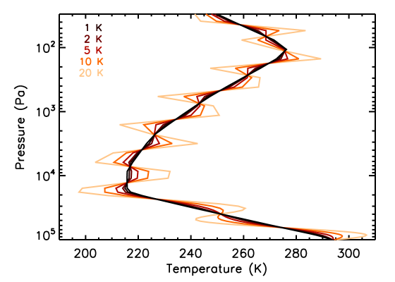
Figure 4: Standard (black) and perturbed (red) temperature profiles used in our validation experiment. Temperature perturbations vary sinusoidally in altitude with an amplitude indicated by shade.

The standard atmosphere we adopt for our validations is a commonly-used atmospheric model for Earth [38]. We include absorption opacity due to water vapor, carbon dioxide, and ozone. Perturbed temperature profiles are generated by adding a sinusoidally-varying component to the standard profile whose periodicity (in altitude) is 7.5 km and whose amplitude is either 1, 2, 5, 10, or 20 K. The standard and perturbed temperature profiles are shown in Figure 4.

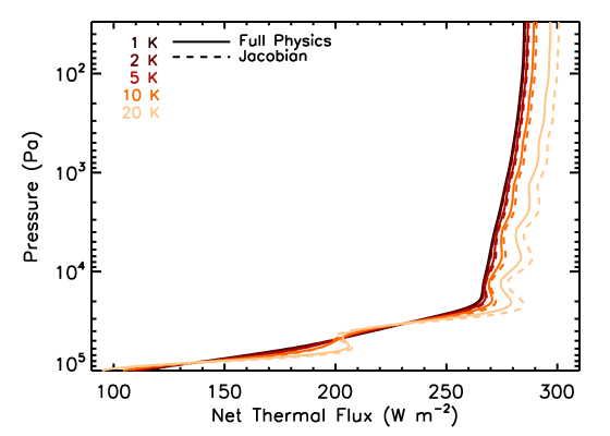
Figure 5: Net thermal flux profiles computed for perturbed temperature profiles (Figure 4) using a full-physics radiative transfer model (solid) and our Jacobian-based method (dashed).

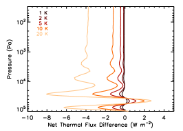
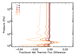
Figure 6: Absolute (left) and fractional (right) differences in net thermal flux profiles computed for perturbed temperature profiles (Figure 4) when comparing our full-physics radiative transfer model and our Jacobian-based method.

Figure 5 shows the net thermal flux profiles computed for our perturbed temperature profiles using both our full-physics model as well as our Jacobian approach. Solar fluxes are largely insensitive to temperature, so are not shown here. For small temperature perturbations (i.e., less than or equal to 5 K), the flux profiles computed via our two different approaches are largely indistinguishable. Figure 6 shows the absolute and relative differences in the net thermal flux profiles when comparing the full-physics or Jacobian-based approaches. Even for 20 K temperature perturbations, the Jacobian-based approach reproduces the full-physics profiles to within 4%. Thus, by removing the Planck-like contribution to our layer thermal source terms, our Jacobian-based approach remains accurate despite large temperature perturbations.

4 Example Applications of the LiFE Approach

In this section we provide three demonstrations, each with increasing complexity, and each touching on a different planet in the Solar System. First, we compute the wavelength-dependent layer radiative properties and their temperature Jacobians for a standard Martian atmosphere. This provides insight into how the layer radiative properties depend on gas and aerosol opacity sources, and how these properties respond to changes in atmospheric temperature. The second demonstration uses the LiFE approach to time-step an Earth-like atmosphere to radiative equilibrium, thus providing an example of how the approach can be used to determine atmospheric thermal structure. The final demonstration uses the LiFE approach and a model of atmospheric convection to time-step a standard Venus atmosphere to radiative-convective equilibrium.

In all cases below, we adopt the SMART model (described above) as our full-physics radiative transfer model. All instances of this tool are run at a sufficiently small wavenumber increments (typically less than 0.01 cm^-1) to resolve all relevant spectral lines between 50 to 10⁵ cm^-1 (i.e., 0.1 to 200 $\mu$m), and, to limit runtime, the resulting layer absorptivities, transmissivities, and source terms are averaged over 5 cm^-1 intervals in the thermal infrared and 10 cm^-1 intervals in the visible. Depending on the complexity of the model atmosphere and the desired number of Jacobians, our full-physics model requires hours to tens of hours to generate the requisite outputs, while subsequently using the LiFE approach to adapt the radiative fluxes towards equilibrium only takes seconds.

4.1 Mars: Layer Radiative Properties and Temperature Jacobians

We use a standard collection of planetary-average atmospheric properties for Mars to compute the layer radiative properties and their Jacobians. We adopt a temperature profile from [39] and a dust optical depth profile from [40]. For simplicity, we assume that the only radiatively active gas is CO₂, which is taken to have a mass mixing ratio of 0.95. Using the SMART model, we generate the layer radiative properties, separating solar and thermal sources, and we also numerically evaluated temperature Jacobians for these properties, assuming a 1% change in temperature at each atmospheric level.

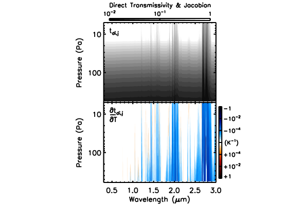
Figure 7: Wavelength-dependent transmissivity for the direct solar beam in the Martian atmosphere (top) and its temperature Jacobian (bottom). For the transmissivity, darker shades indicate low transmission. For the Jacobians, red shades indicate increasing transmissivity with increasing temperature, and blue shades indicate decreasing transmissivity for increasing temperature.

Figure 7 shows the transmissivity for the direct solar flux and the associated temperature Jacobian as shaded contours in wavelength and atmospheric pressure. The transmissivity is dominated by dust opacity at most wavelengths, but CO₂ absorption bands can clearly be distinguished. The Jacobians indicate that the transmissivities are only weakly sensitive to temperature at these wavelengths. An increase in temperature leads to weaker absorption at the centers of absorption bands, and stronger absorption in the wings. This behavior is due to the temperature dependence in the individual line half-widths (which are predominately Doppler broadened here), and the Boltzmann-like temperature dependence in the line strengths, both of which lead to decreased opacity (increased transmissivity) near band centers for increased temperature. Note that absorption in the centers of some CO₂ bands are so strong in the deepest portions of the atmosphere that their transmissivity is zero for all temperatures used in these models, and so the Jacobians show no temperature sensitivity here.

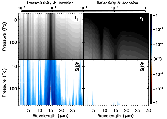
Figure 8: Wavelength-dependent layer diffuse flux transmissivity (top-left) and reflectivity (top-right) in the Martian atmosphere and their temperature Jacobians (bottom). For the transmissivity and its Jacobian, shading is the same as in Figure 7. For the reflectivity, lighter shades indicate higher layer reflectance, and, for the Jacobians, red shades indicate increasing reflectivity with increasing temperature, while blue shades indicate decreasing reflectivity for increasing temperature.

Layer diffuse flux transmissivity and reflectivity, as well as their associated temperature Jacobians, are shown in Figure 8. As was the case for the direct solar flux, the transmissivity is dominated by dust opacity except in the CO₂ absorption bands, with the 4.3 $\mu$m and 15 $\mu$m bands being especially absorptive. Layer reflectivity is generally small, and drops to zero at the centers of strong CO₂ features. Like the direct solar terms, the transmissivity Jacobians show that increased temperatures cause decreased absorption near band centers, and increased absorption in band wings. Due to the increased absorption in band wings at higher temperatures, the reflectivity decreases at these wavelengths as temperature increases.

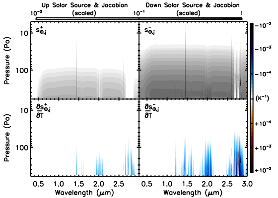
Figure 9: Wavelength-dependent upwelling (left) and downwelling (right) layer solar source terms (top) and their temperature derivatives (bottom) for Mars. Both the source terms and their derivatives have been scaled by (1) the top-of-atmosphere solar flux, which removes wavelength-dependent structure from the solar spectrum, and (2) $d\ln p_{j}$, which removes layer path length effects and creates source terms that are smooth functions of pressure. For the source terms, darker shades indicate larger flux sources. For the Jacobians, red shades indicate increasing sources with increasing temperature, and blue shades indicate decreasing sources with increasing temperature.

Figure 9 shows the layer solar source terms, which have been adjusted by the top-of-atmosphere solar flux to remove wavelength-dependent structure resulting from the solar spectrum. As the dust particles are forward-scattering, the downwelling solar source terms tend to be larger than the upwelling source terms. Wavelength-dependent structure in both the upwelling and downwelling source terms is due primarily to the dust optical properties, which have a lower single-scattering albedo below about 0.6 $\mu$m. Note that the source terms are smaller (or vanishingly small) within CO₂ absorption features, since the layers strongly absorb sunlight at these wavelengths, rather then scattering it into the diffuse radiation field. Finally, the temperature Jacobians show a decrease in the source terms for an increase in temperature in the wings of CO₂ features, and an increase in the cores. This is due to the decrease in transmissivity in band wings at higher temperatures, and the increase in transmissivity in the band cores.

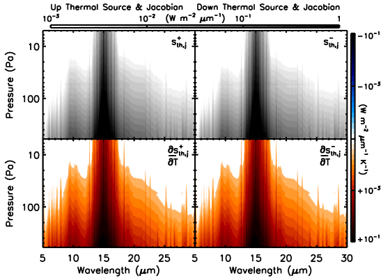
Figure 10: Wavelength-dependent upwelling (left) and downwelling (right) layer thermal source terms (top) and their temperature derivatives (bottom) for Mars. For the source terms, darker shades indicate larger flux sources. For the Jacobians, red shades indicate increasing sources with increasing temperature, and blue shades indicate decreasing sources with increasing temperature.

Layer thermal sources are shown in Figure 10. The upwelling and downwelling terms are identical since the layers are equally efficient at generating upwelling and downwelling thermal flux. The sources are strongest in the 15 $\mu$ CO₂ band, with dust providing thermal radiative fluxes outside of CO₂ features. As one might expect, the temperature Jacobians (shown at the bottom of this figure) demonstrate that, for an increase in temperature, the layer thermal source terms increase at all wavelengths.

4.2 Earth: Using LiFE to Determine Radiative Equilibrium Thermal Structure

An important aspect of the LiFE approach is that it allows the radiative fluxes in a planetary atmosphere to be rapidly adapted to changes in the atmospheric state, while still being guided by the values from the full-physics model. Thus, the approach can be used to estimate the solar and thermal flux variations that occur as the thermal structure evolves from an initial state toward thermal equilibrium. As a demonstration, in this section we use the LiFE approach to determine the radiative equilibrium thermal structure of an Earth-like atmosphere.

We assume an atmosphere that is 78% N₂ and 21% O₂, by volume, and we include H₂O, CO₂, and O₃ as trace gases. In reality, water vapor is a condensible species in Earth’s atmosphere, whose partial pressure is tied to atmospheric temperature. However, for simplicity, we hold the water vapor mixing ratio profile fixed. For this example, we do not include clouds, and we assume a wavelength-dependent surface albedo appropriate for ocean (which has a value of  5% at most wavelengths).

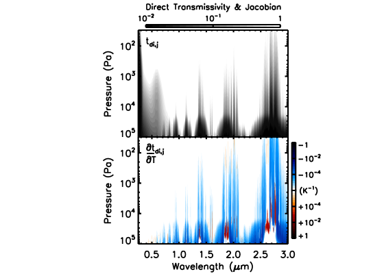
Figure 11: Initial wavelength-dependent transmissivity for the direct solar beam in Earth’s atmosphere (top) and its temperature Jacobian (bottom) used in our example application of the LiFE approach. Shading is the same as Figure 7.

Direct solar transmissivity and its temperature Jacobian are shown in Figure 11. Strong absorption features due to water vapor can be seen throughout the near-infrared, contributions from CO₂ can be seen near 2.2 and 2.7 $\mu$m, and opacity from ozone and Rayleigh scattering are apparent at shorter wavelengths. Our extinction cross sections for ozone and Rayleigh scattering in the ultraviolet and visible are not temperature dependent, so these features do not appear in the temperature Jacobians. The water vapor absorption bands show a similar temperature dependence to the absorption bands seen for Mars in the previous section.

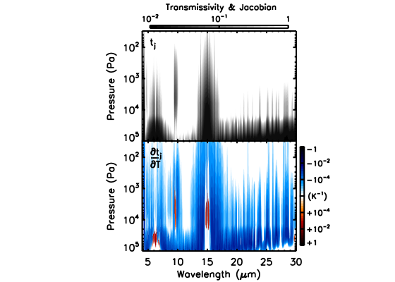
Figure 12: Initial wavelength-dependent layer diffuse flux transmissivity (top) in Earth’s atmosphere and its temperature Jacobian (bottom) used in our example application of the LiFE approach. Shading is the same as Figure 8. Layer reflectivity is not shown as reflectance is due to Rayleigh scattering and, thus, is effectively zero at the wavelengths used above.

Layer transmissivity and its temperature Jacobian throughout the mid-infrared are shown in Figure 12. Layer reflectivity is not shown as it is uniformly zero at these wavelengths. Line absorption due to H₂O, CO₂, and O₃ can be clearly distinguished. Like the Mars example, each band shows an increasing transmissivity with temperature at its core, and a decreasing transmissivity with temperature in its wings. This effect is due, predominately, to the temperature dependence in line strengths.

Solar sources are shown in Figure 9, which are due to Rayleigh scattering. Again, temperature Jacobians are not shown as the Rayleigh scattering extinction cross section does not depend on temperature in our model. Thermal sources and their temperature Jacobians are shown in Figure 10. As would be expected, the sources show that thermal flux is mostly generated in water vapor, carbon dioxide, and ozone absorption bands, and the flux increases with temperature.

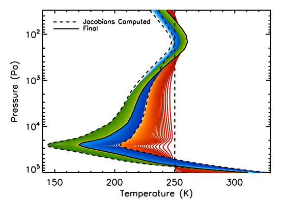
Figure 15: Evolution of our 1-D, cloud-free Earth atmosphere to a radiative equilibrium state, beginning with an isothermal profile (dashed). Red curves show the evolution using the first set of computed layer radiative properties and their Jacobians, with lighter hues indicates later times, which ends at the dashed profile. Our full-physics model is then used to compute updated layer radiative properties and Jacobians for this new atmospheric state and evolved through time, as is shown by the blue curves (resulting in the temperature profile with the coldest tropopause). This process is repeated again, following the green curves with time. The final profile is the solid line in black.

To determine the radiative equilibrium thermal structure of the atmosphere we solve the thermodynamic energy equation as an initial value problem. Our calculation begins with an isothermal profile for which we generate the layer source terms and their temperature Jacobians. We then use these to time-step the atmosphere to radiative equilibrium by using the radiative heating/cooling rates to update the temperature profile, and then using the LiFE approach to determine the radiative fluxes for the updated atmospheric state. This temperature evolution of the atmosphere away from the isothermal state is shown by the red profiles in Figure 15, and the resulting radiative equilibrium solution is the dashed line. Recall that this is a pure radiative equilibrium solution, and not a radiative-convective solution, thus resulting in a very cold tropopause. The initial full-physics calculation takes about two wall clock hours on a single processor, and each time step using the Jacobians takes about one second. The progression to radiative equilibrium from the isothermal state takes 2,000 time steps, which translates to five months of model time.

The solution found by application of the first set of Jacobians is not the true radiative equilibrium solution, since the temperature profile has evolved away from the range over which the Jacobians are valid. So, we twice repeat the process outlined in the previous paragraph, resulting in evolution shown by the blue and green profiles in Figure 15. Since each iteration is nearer to the true radiative equilibrium solution, the number of time steps required to reach equilibrium is less than the first iteration. Model timescales to reach equilibrium for the second and thirds iterations were four months and one month, respectively.

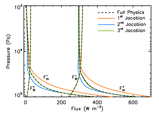
Figure 16: Evolution of upwelling and downwelling solar and thermal flux profiles, following Figure 15. Dashed lines show the radiative-equilibrium profiles, as computed by the full-physics model. Colored curves show the profiles for the different radiative-equilibrium states determined by successive refinements of the layer radiative properties and their Jacobians.

The accuracy of the three sets of layer radiative properties and their associated Jacobians in computing the radiative equilibrium solution can be seen by comparing the solar and thermal flux profiles to those computed by the full-physics model. Figure 16 demonstrates how the different sets of radiative properties and Jacobians approach the true solution. Upwelling and downwelling solar and thermal flux profiles are shown, with the “true" radiative equilibrium solution (from the full-physics model) shown as dashed lines. All sets of layer radiative properties and Jacobians do a good job of matching the solar flux profiles, which are largely insensitive to changes in atmospheric temperature. However, the thermal fluxes from the radiative equilibrium solution determined from the first set of properties and Jacobians differ from the true fluxes by more than 50 W m^-2 at some pressures. This difference shrinks to nearly zero through subsequent computations of properties and Jacobians, eventually arriving at the correct solution.

4.3 Venus: Determining the Radiative-Convective Equilibrium State with the LiFE Approach

The structure of real planetary atmospheres depends on more than just radiative balance—dynamical processes, such as convection, are also of critical importance. To demonstrate how the LiFE approach works within a 1-D radiative-convective scheme, we paired the SMART model and the associated LiFE framework with a simple mixing-length approach to convection. Here, the convective heating rate, $q_{c}$, is given by

$$q_{c}=-\frac{1}{c_{p}\rho}\frac{dF_{c}}{dz}\ ,$$ (29)

where $c_{p}$ is the atmospheric heat capacity, $\rho$ is the atmospheric density, and $F_{c}$ is the convective heat flux, taken as

$$F_{c}=-\rho c_{p}K_{H}\left(\frac{dT}{dz}+\Gamma_{ad}\right)\ ,$$ (30)

where $K_{H}$ is the eddy diffusivity for heat, and $\Gamma_{ad}=g/c_{p}$ is the adiabatic lapse rate, where $g$ is the acceleration due to gravity. The eddy diffusivity vanishes when the temperature profile is stable against convection, and is given by

$$K_{H}=\begin{cases}l^{2}\left[-\frac{g}{T}\left(\frac{dT}{dz}+\Gamma_{ad}\right)\right]^{1/2},&\frac{dT}{dz}>-\Gamma_{ad}\\ 0,&\frac{dT}{dz}\leq-\Gamma_{ad}\end{cases}$$ (31)

where $l$ is the mixing length. We follow Blackadar [41], taking the mixing length to be

$$l=\frac{kz}{1+kz/l_{0}}\ ,$$ (32)

where $k$ is von Kármán’s constant, and $l_{0}$ is the mixing length in the free atmosphere, which we take as the pressure scale heigh, $H=RT/g$, where $R$ is the specific gas constant.

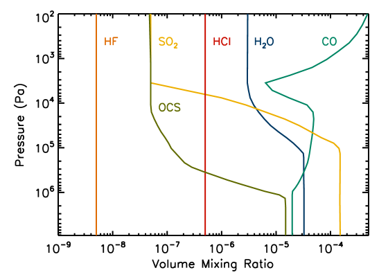
Figure 17: Gas mixing ratio profiles used in our Venus thermal structure calculations, from Haus et al. [42].

We take the atmosphere to be 96% CO₂ and 4% N₂, by volume, and we include H₂O, HDO (whose mixing ratio relative to the primary isotopologue is taken to be 130$\times$ larger than the telluric value), SO₂, CO, OCS, HCl, and HF as trace gases. The mixing ratios for our trace gases, as well as our treatment of the “unknown UV absorber”, are taken from the Haus et al. [42], and gas mixing ratio profiles are shown in Figure 17. We use a standard collection of cloud optical properties and vertical distributions, which are taken from Crisp [20]. Collisional line mixing is understood to alter CO₂ lineshapes to be sub-Lorentzian at high pressures, which we parameterize through a standard set of $\chi$ factors defined in [33]. Our treatment of collision induced absorption stems from a number of sources [43, 44, 45, 46]. We use HITEMP 2010 [47] for our water vapor linelist, Huang et al. [48] for our carbon dioxide linelist, and HITRAN 2012 [49] for all other gases.

To decrease runtime, model time stepping began with an initial $T$-$p$ profile that had a surface temperature of 730 K, following a dry adiabat to 0.1 bar, and an isothermal upper atmosphere at 210 K. Initial profiles further from the equilibrium solution were also found to approach the same solution as the case presented here, but require substantially more iterations of the full-physics model. To expedite the march to equilibrium, we use a pressure-dependent time step, which helps account for the long thermal timescales that occur deep in the Venusian atmosphere. A functional form that was found to work had $\Delta t\propto p^{1/4}$.

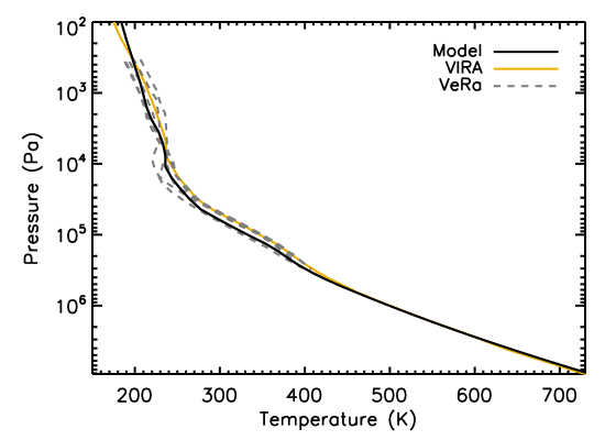
Figure 18: Venus radiative-convective equilibrium thermal structure from our model. Also shown is the Venus International Reference Atmosphere (VIRA) [50] and a number of latitude-dependent temperature profiles for the upper atmosphere from the Venus Express radio science experiment (VeRa) [51], spanning the equatorial region to high latitudes.

A total of three sets of full-physics calculations were used to achieve a radiative-convective equilibrium state, and shortwave fluxes were computed at four Gaussian solar zenith angles covering the sunlit hemisphere and were combined using Gaussian quadrature [20]. While using multiple solar zenith angles increases runtime, this approach helps to ensure a better “planetary average” set of shortwave fluxes. Our equilibrium radiative-convective profile is shown in Figure 18. As our initial guess was near the final answer, the temperature evolution of the atmosphere was less dramatic than in the Earth case, so we only show the final $T$-$p$ profile in this figure. Also shown are the Venus International Reference Atmosphere (VIRA) [50] and measurements of the mesospheric thermal structure from Venus Express [51].

The model reproduces the thermal structure of the Venusian atmosphere extremely well. Our computed surface temperature is 736 K, which is consistent with the ground-truthed value of $\sim\!735$ K derived from Pioneer Venus and the Venera landers [52]. Critically, our computed mesospheric thermal structure is bounded by the radio occultation results from Venus Express.

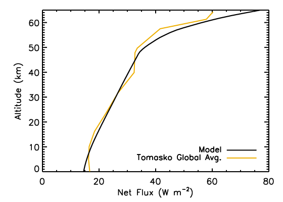
Figure 19: Net solar flux in the Venus atmosphere from our model (black) and from an estimate of the global average from Tomasko et al. [53] (yellow), which was based on measurements from the Pioneer Venus sounder.

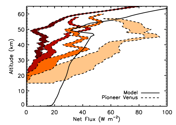
Figure 20: Net thermal flux in the atmosphere of Venus. Solid line is from our model, and shaded regions represent measurements and uncertainties from the Pioneer Venus sounder and probes [from 54]. From left to right at 40 km, data curves are: sounder, day-side, 4^∘ N; probe, day-side, 31^∘ S; probe, night-side, 27^∘ S; and probe, day-side, 60^∘ N.

Solar flux profiles from the radiative-convective equilibrium model are shown in Figure 19. Also shown is an estimate of the global average net flux profile, which is based on results from the Pioneer Venus sounder [53]. The model shortwave profiles are in excellent agreement with the data. Finally, the model net thermal flux profile is shown in Figure 20. Measurements and uncertainty estimates from the Pioneer Venus mission are also shown, and are taken from Revercomb et al. [54]. In general, the model falls within the range of measured values, although there is an indication that the model finds a larger net thermal flux profile in the deepest regions of the atmosphere (i.e., below about 15 km). Observations of the Venus night side [55, 33, 56] indicate that much of the variability in the Pioneer Venus net thermal fluxes may be associated with variations in the highly-variable thermal infrared opacity of the middle and lower clouds [57], an effect omitted in our calculations. The sudden decrease in net thermal flux near 50 km altitude is due to convection at the cloud base in our simulation.

Recently, Haus et al. [58] applied a Jacobian-based technique to computing solar heating and thermal cooling rates in the Venusian mesosphere. In this approach, individual level temperatures (or some other quantity, such as a cloud enhancement parameter) were perturbed, and a new net heating/cooling rate was calculated at all model layers using a full-physics model. Jacobians, which describe the response of a layer heating/cooling rate to a change in temperature (or some other parameter) at any given model level, were determined by differencing the perturbed cases to a baseline model. This approach has the computational advantage of being spectrally-unresolved (as heating/cooling rates are integrated quantities), although a wavelength/wavenumber grid correction factor was required to be applied to the Jacobian-computed heating/cooling rates. The LiFE approach, while spectrally-resolved, has the advantage that Jacobians are computed on local layer radiative properties, and perturbations to the atmosphere are then handled using radiative principles (i.e., a two-stream flux adding technique). Temperature sensitivity is significantly reduced (see Section 3) by removing a Planck-like contribution to the layer source terms (i.e., Equations 23 and 24), which would not be the case when working with heating/cooling rate Jacobians. Furthermore, the heating/cooling rate approach described by Haus et al. scales as the square of the number of atmospheric layers, whereas the LiFE approach scales linearly with the number of atmospheric layers (and with the number of spectral gridpoints).

5 Example Model Comparison

We further explore the accuracy of our climate calculations via a comparison to a widely-adopted, one-dimensional radiative convective model—the Clima tool developed by Kasting and collaborators [59, 60, 61, 62]. As with our Venus simulations, we adopt (i) the SMART model as our full-physics tool for computing requisite layer radiative properties and their Jacobians, (ii) the LiFE approach to adapting radiative fluxes to changes in atmospheric structure as the simulation timesteps to equilibrium, and (iii) a mixing-length approach to convective heat transport. The case the we simulate is a planet with a 1 bar pure carbon dioxide atmosphere orbiting at 1 au from the Sun. The world has an identical radius to Earth, a surface gravity of 10 m s^-2, and a gray surface albedo of 0.20. Both models compute a planetary average solar heating rate using eight solar zenith angles. The LiFE-based approach began with a 250 K isothermal atmospheric temperature profile, and used two calls to the full-physics model to determine the layer radiative properties and their temperature derivatives.

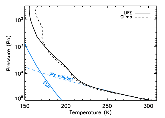
Figure 21: Comparison of the equilibrium radiative-convective thermal structures computed using the Clima model and our LiFE-based approach for a planet with a 1 bar pure carbon dioxide atmosphere orbiting at 1 AU from a solar twin. The dry adiabat and saturation vapor pressure (SVP) are shown for carbon dioxide.

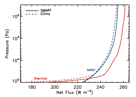
Figure 22: Net solar (blue) and thermal (red) flux profiles computed for the Clima-derived equilibrium thermal structure shown in Figure 21. Flux profiles were computed using the SMART full-physics model (solid) and the radiative transfer routines adopted in the Clima model (dashed).

The equilibrium thermal structures determined by Clima and our LiFE-based approach are shown in Figure 21. Both models find a surface temperature of 310 K. The thermal structure profiles are also in agreement, although the Clima model finds additional structure in the radiative portion of the profile as well as an upper stratosphere that is warmer by about 10 K. For the equilibrium thermal structure determined by the Clima model, Figure 22 shows the net solar and thermal flux profiles as computed by the Clima and SMART models, whose core radiative transfer routines were last inter-compared by Kopparapu et al. [61]. The net solar flux profiles from these two models are in good agreement. The net thermal flux profiles, however, show some more substantial differences, including a 6 W m^-2 discrepancy at the top of the atmosphere. The net flux profile from the SMART full-physics model yields strong cooling above 300 Pa, and, in general, heating between 300 Pa and the top of the convective zone. These heating/cooling trends would work to bring the Clima-derived thermal structure into closer agreement with the LiFE-derived temperature-pressure profile.

A key characteristic of the Clima model is its relatively short runtime—equilibrium thermal structures can typically be determined in minutes, or within an hour for more complicated scenarios. This can be compared to runtimes for the LiFE approach, where computation of layer radiative properties and their Jacobians using a full-physics model takes hours to tens of hours (depending on complexity), and the process of timestepping towards an equilibrium solution can take several hours (although a single call to our two-stream flux adding routines only takes seconds). An asset of the LiFE approach is versatility, however, as a huge variety of gases and/or aerosols can be straightforwardly incorporated into simulations (without needing to compute associated $k$-coefficients, for example), and runtimes only scale linearly (or better) with the number of added gases. Furthermore, the LiFE approach benefits from having its radiative flux profiles being grounded in a full-physics radiative transfer tool. Nevertheless, the LiFE approach would certainly benefit from updates focused on decreasing model runtime. These updates could include implementing analytic Jacobians within the full-physics model used to compute layer radiative properties and their derivatives [32], as well as an implementation of a root finding algorithm for determining equilibrium atmospheric states (as opposed to our current time-stepping algorithm).

6 Summary

Planetary climate models require accurate radiative fluxes that can be easily and quickly updated in response to changes in the atmospheric and surface state. We have described a technique — the Linearized Flux Evolution (LiFE) approach — that pairs a full-physics radiative transfer model with an efficient two-stream flux adding scheme to rapidly and accurately adapt radiative flux profiles to state variations. The full-physics model is responsible for compiling the optical properties of the surface and atmosphere, solving for the angle- and level-dependent radiation field, determining the transmissivity, absorptivity, and source terms for each atmospheric layer (which, collectively, we call the layer radiative properties), and also computing Jacobians for these layer radiative properties with respect to any variable aspects of the atmospheric and surface state. We believe this model to be the first of its kind, although recent work in the pure-absorption limit has used a line-by-line approach to computing radiative fluxes in proposed atmospheres for early Mars [63].

Using linear theory and the Jacobians, we update the computed layer radiative properties to small changes in the atmospheric and surface state. While radiances are known to be a strongly non-linear function of the state, the use of quasi-monochromatic layer radiative properties helps to improve the linearity of the problem. Additionally, for the atmospheric temperature component of the state vector, we use an analytic approach to remove the non-linear Planck-derived portion of layer thermal source terms. Layer radiative properties that have been updated to reflect a change in the atmospheric and surface state can then be translated into new radiative flux profiles using the two-stream adding technique we describe.

By applying the LiFE approach to Mars, Earth, and Venus, we demonstrate its versatility. For Mars, we derive and show examples of the layer radiative properties and their temperature Jacobians. Then, for Earth, we allow the thermal structure to evolve in time, demonstrating how LiFE can be used to timestep an atmospheric to pure radiative equilibrium. Finally, our application of LiFE to Venus shows how the approach can be used within a 1-D radiative-convective model. Using mixing length theory to compute the convective fluxes and LiFE to find the radiative fluxes, we determine an equilibrium thermal structure and for Venus, and net solar and thermal flux profiles, that strongly resemble observations. Given these successful applications, we hope that the LiFE approach will prove useful to many problems in planetary and Earth science.

Appendix

I Deriving the Flux Adding Relations

i Combining Two Homogenous Layers

We can write a set of expressions, similar to Equations 1 and 2, for layer $j+1$ as

$$F^{+}_{j}=r_{j+1}F^{-}_{j}+t_{j+1}F^{+}_{j+1}+s^{+}_{j+1}\ ,$$ (33)

$$F^{-}_{j+1}=t_{j+1}F^{-}_{j}+r_{j+1}F^{+}_{j+1}+s^{-}_{j+1}\ .$$ (34)

Combining layers $j$ and $j+1$ yields an inhomogeneous layer, with emergent fluxes $F^{+}_{j-1}$ and $F^{-}_{j+1}$ and incident fluxes $F^{-}_{j-1}$ and $F^{+}_{j+1}$. We can use Equations 2 and 33 to eliminate $F^{-}_{j}$ and $F^{+}_{j}$ from Equations 1 and 34, which yields

$$\begin{array}[]{ll}F^{+}_{j-1}=&\left(r_{j}+\frac{r_{j+1}t_{j}^{2}}{1-r_{j}r_{j+1}}\right)F^{-}_{j-1}+\frac{t_{j}t_{j+1}}{1-r_{j}r_{j+1}}F^{+}_{j+1}\\ &+\frac{t_{j}r_{j+1}}{1-r_{j}r_{j+1}}s^{-}_{j}+\frac{t_{j}}{1-r_{j}r_{j+1}}s^{+}_{j+1}+s^{+}_{j}\ ,\end{array}$$ (35)

$$\begin{array}[]{ll}F^{-}_{j+1}=&\frac{t_{j}t_{j+1}}{1-r_{j}r_{j+1}}F^{-}_{j-1}+\left(r_{j+1}+\frac{r_{j}t_{j+1}^{2}}{1-r_{j}r_{j+1}}\right)F^{+}_{j+1}\\ &+\frac{t_{j+1}}{1-r_{j}r_{j+1}}s^{-}_{j}+\frac{r_{j}t_{j+1}}{1-r_{j}r_{j+1}}s^{+}_{j+1}+s^{-}_{j+1}\ .\end{array}$$ (36)

Equations 35 and 36, which encompass two homogenous layers, are in the form of the relations for a single layer (e.g., Equations 1 and 2), and can be written as

$$F^{+}_{j-1}=R_{j,j+1}^{+}F^{-}_{j-1}+T_{j,j+1}^{+}F^{+}_{j+1}+S_{j,j+1}^{+}\ ,$$ (37)

$$F^{-}_{j+1}=T_{j,j+1}^{-}F^{-}_{j-1}+R_{j,j+1}^{-}F^{+}_{j+1}+S_{j,j+1}^{-}\ ,$$ (38)

where we have defined the properties of an inhomogeneous layer encompassing layers $j$ and $j+1$ as

$$R_{j,j+1}^{+}=r_{j}+\frac{r_{j+1}t_{j}^{2}}{1-r_{j}r_{j+1}}\ ,$$ (39)

$$T_{j,j+1}^{+}=\frac{t_{j}t_{j+1}}{1-r_{j}r_{j+1}}\ ,$$ (40)

$$R_{j,j+1}^{-}=r_{j+1}+\frac{r_{j}t_{j+1}^{2}}{1-r_{j}r_{j+1}}\ ,$$ (41)

$$T_{j,j+1}^{-}=\frac{t_{j}t_{j+1}}{1-r_{j}r_{j+1}}\ ,$$ (42)

$$S_{j,j+1}^{+}=\frac{t_{j}r_{j+1}}{1-r_{j}r_{j+1}}s^{-}_{j}+\frac{t_{j}}{1-r_{j}r_{j+1}}s^{+}_{j+1}+s^{+}_{j}\ ,$$ (43)

$$S_{j,j+1}^{-}=\frac{t_{j+1}}{1-r_{j}r_{j+1}}s^{-}_{j}+\frac{r_{j}t_{j+1}}{1-r_{j}r_{j+1}}s^{+}_{j+1}+s^{-}_{j+1}\ .$$ (44)

Unlike a homogenous layer, the combined inhomogeneous layer does not reflect or transmit upwelling and downwelling fluxes symmetrically, as is indicated by the “+” and “-” superscripts on the inhomogeneous layer reflectivity and transmissivity. The ability of a homogenous layer to reflect (or transmit) flux doesn’t depend on whether it is illuminated from above or below. For a inhomogeneous layer, though, it can, for example, be more effective at reflecting (or transmitting) flux that is incident from below than flux that is incident from above.

ii Adding a Homogenous Layer to the Base of an Inhomogeneous Layer

In downward adding, we determine the radiative properties of successfully thicker inhomogeneous layers by recursively adding a homogenous layer to the base of an inhomogeneous layer. For homogenous layer $j$, Equations 1 and 2 are still valid. For the inhomogeneous layer extending from the top of the atmosphere ($j=0$) to layer $j-1$, we define the inhomogeneous layer reflectivity and source term for adding downward, $R^{-}_{0,j-1}$ and $S^{-}_{0,j-1}$, in Equation 3. Note that the contribution to the downwelling flux from the top-of-atmosphere boundary condition (i.e., $F^{-}_{0}$) can be included in the source term at the top of the atmosphere, $s^{-}_{0}=S^{-}_{0,0}$.

Inserting Equation 1 into the right hand side of Equation 3 and simplifying yields

$$F^{-}_{j-1}=\left(t_{j}R^{-}_{0,j-1}F_{j}^{+}+s^{+}_{j}R^{-}_{0,j-1}+S^{-}_{0,j-1}\right)/\left(1-r_{j}R^{-}_{0,j-1}\right)\ ,$$ (45)

and inserting this into Equation 2 gives us

$$F^{-}_{j}=\left(r_{j}+\frac{t_{j}^{2}R^{-}_{0,j-1}}{1-r_{j}R^{-}_{0,j-1}}\right)F_{j}^{+}+s^{-}_{j}+\frac{t_{j}\left(S^{-}_{0,j-1}+s^{+}_{j}R^{-}_{0,j-1}\right)}{1-r_{j}R^{-}_{0,j-1}}\ .$$ (46)

Note that this is in a similar form to Equation 3, and can be written as

$$F^{-}_{j}=R^{-}_{0,j}F_{j}^{+}+S^{-}_{0,j}\ ,$$ (47)

with $R^{-}_{0,j}$ and $S^{-}_{0,j}$ defined as in Equations 4 and 5, respectively.

For an entire model atmosphere, downward layer adding begins with the top homogenous layer and a pair of boundary conditions (for $r_{0}$ and $s^{-}_{0}$), following the description in Section I(i). Adding these two layers yields the quantities $R_{0,1}^{-}$ and $S_{0,1}^{-}$ for an inhomogeneous layer. Equations 4 and 5 then provide a recursive set of relations that define the reflectivity and source terms of successfully thicker inhomogeneous layers for downward adding.

iii Adding a Homogenous Layer to the Top of an Inhomogeneous Layer

Upward adding proceeds in a similar fashion to downward adding, except that homogenous layers are added to the top of inhomogeneous layers. Again, Equations 1 and 2 are still valid for homogenous layer $j$. For the inhomogeneous layer extending from the base of the atmosphere ($j=N-1$) to the bottom of layer $j$, we have Equation 6, which defines the inhomogeneous layer reflectivity and source term for adding upward ($R_{j+1,N}^{+}$ and $S_{j+1,N}^{+}$, respectively).

Inserting Equation 2 into Equation 6 and simplifying yields

$$F_{j}^{+}=\left(t_{j}R_{j+1,N}^{+}F_{j-1}^{-}+s_{j}^{-}R_{j+1,N}^{+}+S_{j+1,N}^{+}\right)/\left(1-r_{j}R_{j+1,N}\right)\ .$$ (48)

Inserting this equality for $F_{j}^{+}$ into Equation 1 and simplifying then gives us

$$F_{j-1}^{+}=\left(r_{j}+\frac{t_{j}^{2}R^{+}_{j+1,N}}{1-r_{j}R^{+}_{j+1,N}}\right)F_{j-1}^{-}+s^{+}_{j}+\frac{t_{j}\left(S^{+}_{j+1,N}+s^{-}_{j}R^{+}_{j+1,N}\right)}{1-r_{j}R^{+}_{j+1,N}}\ .$$ (49)

This is in a similar form to Equation 6, and can be written as

$$F_{j-1}^{+}=R_{j,N}^{+}F_{j-1}^{-}+S_{j,N}^{+}\ ,$$ (50)

with the recursive definitions for $R_{j,N}^{+}$ and $S_{j,N}^{+}$ given by Equations 7 and 8, respectively.

Beginning with the bottom homogenous layer of the atmosphere and a pair of boundary conditions (for $r_{N}$ and $s_{N}^{+}$), we produce an inhomogeneous layer according to the description in Section I(i), thus yielding the quantities $R_{N-1,N}^{+}$ and $S_{N-1,N}^{+}$. Equations 7 and 8 then provide a recursive set of relations that define the reflectivity and source terms of successfully thicker inhomogeneous layers for upward adding.

II Worked Example of Flux Adding and Linearized Evolution

The flux adding scheme outlined in Section 2.1 is typically performed at a particular wavelength within a spectral interval. However, insight can be gained by applying the flux adding method in a case where the optical properties of the atmosphere are gray (i.e., independent of wavelength). For simplicity, we only consider thermal sources and we ignore scattering in this example. Also, we stress that the example below is designed to build intuition, and is not representative of the more complex approach described and used in this manuscript.

We divide the atmosphere into $N-1$ layers, with boundaries at gray thermal optical depths given by $\tau_{0}$, $\tau_{1}$, … $\tau_{N-1}$, with $\tau_{N-1}=\tau^{*}$, where $\tau^{*}$ is the total gray infrared optical depth of the atmosphere. Note that we have included the diffusivity factor scaling [64, 65] in our definition of the optical depth. We take the flux transmissivity of layer $j$ to be given by

$$t_{j}=e^{-\Delta\tau_{j}}\ ,$$ (51)

where $\Delta\tau_{j}=\tau_{j}-\tau_{j-1}$, and a simple expression of the layer source terms could be taken as

$$s^{+,-}_{j}=\left(1-e^{-\Delta\tau_{j}}\right)\sigma\bar{T}^{4}_{j}\ ,$$ (52)

where $\bar{T}_{j}$ is a representative average temperature of layer $j$, and the term in parentheses is the layer emissivity. Note that, here, we have assumed a functional form for the layer source terms, whereas in the manuscript above these are determined via comparisons to a full-physics model.

By construction, the reflectivity of each layer is zero (i.e., $r_{j}=0$), which greatly simplifies the adding approach, giving

$$\begin{array}[]{lr}R^{+}_{j,N}=R^{-}_{0,j}=0&\forall j\ .\end{array}$$ (53)

By inserting this into Equations 47 and 9, we see that the upwelling and downwelling thermal fluxes (in this example) are simply given by the upward and downward adding source terms for the inhomogeneous layers,

$$F^{-}_{j}=S^{-}_{0,j}$$ (54)

$$F_{j}^{+}=S^{+}_{j+1,N}\ .$$ (55)

Additionally, the recursive relationships for the inhomogeneous layer source terms (Equations 5 and 8) simplify to

$$S^{-}_{0,j}=s^{-}_{j}+t_{j}S^{-}_{0,j-1}$$ (56)

$$S_{j,N}^{+}=s^{+}_{j}+t_{j}S^{+}_{j+1,N}\ .$$ (57)

When adding downwards, we start with the boundary condition that the downwelling thermal flux at the top of the atmosphere is zero,

$$F^{-}_{0}=S^{-}_{0,0}=0\ .$$ (58)

We then use Equation 56 to find:

$$\begin{array}[]{ccccl}S^{-}_{0,1}&=&s^{-}_{1}+t_{1}S^{-}_{0,0}&=&\left(1-e^{-\Delta\tau_{1}}\right)\sigma\bar{T}^{4}_{1}\\ S^{-}_{0,2}&=&s^{-}_{2}+t_{2}S^{-}_{0,1}&=&\left(1-e^{-\Delta\tau_{2}}\right)\sigma\bar{T}^{4}_{2}+e^{-\Delta\tau_{2}}\left(1-e^{-\Delta\tau_{1}}\right)\sigma\bar{T}^{4}_{1}\\ &&&\vdots&\\ S^{-}_{0,N-1}&=&s^{-}_{N-1}+t_{N-1}S^{-}_{0,N-2}&=&\left(1-e^{-\Delta\tau_{N-1}}\right)\sigma\bar{T}^{4}_{N-1}+e^{-\Delta\tau_{N-1}}\times\dots\end{array}$$ (59)

Similarly, when adding upwards, we begin with the boundary condition that the upwelling flux at the base of the atmosphere is just the thermal flux from the surface,

$$F_{N-1}^{+}=S^{+}_{N,N}=\sigma T_{s}^{4}\ ,$$ (60)

and use Equation 57 to find:

$$\begin{array}[]{ccccl}S^{+}_{N-1,N}&=&s^{+}_{N-1}+t_{N-1}S^{+}_{N,N}&=&\ \left(1-e^{-\Delta\tau_{N-1}}\right)\sigma\bar{T}^{4}_{N-1}+e^{-\Delta\tau_{N-1}}\sigma T_{s}^{4}\\ S^{+}_{N-2,N}&=&s^{+}_{N-2}+t_{N-2}S^{+}_{N-1,N}&=&\ \left(1-e^{-\Delta\tau_{N-2}}\right)\sigma\bar{T}^{4}_{N-2}+e^{-\Delta\tau_{N-2}}\times\\ &&&&\left[\left(1-e^{-\Delta\tau_{N-1}}\right)\sigma\bar{T}^{4}_{N-1}+\sigma T_{s}^{4}e^{-\Delta\tau_{N-1}}\right]\\ &&&\vdots&\\ S^{+}_{1,N}&=&s^{+}_{1}+t_{1}S^{+}_{2,N}&=&\ \left(1-e^{-\Delta\tau_{1}}\right)\sigma\bar{T}^{4}_{1}+e^{-\Delta\tau_{1}}\times\dots\end{array}$$ (61)

The key element of the state vector in this example is the atmospheric temperature profile. To determine how the flux profiles respond to changes in the temperature profile, we evaluate the derivatives of Equations 51 and 52 with respect to $\bar{T}_{j}$. This gives us

$$\frac{\partial t_{j}}{\partial\bar{T}_{j}}=0\ ,$$ (62)

$$\frac{\partial s^{+,-}}{\partial\bar{T}_{j}}=4\left(1-e^{-\Delta\tau_{j}}\right)\sigma\bar{T}^{3}_{j}\ .$$ (63)

In this example, the layer source term derivatives are analytic, and have a strong temperature dependence.

To proceed any further, we need to specify an atmospheric temperature profile, $T(\tau)$. For simplicity, we adopt the radiative equilibrium temperature profile obtained by solving the two-stream Schwarzschild equation for the thermal radiative fluxes in a planetary atmosphere [66, p. 84], under the assumption that the atmosphere in transparent to shortwave radiation and that the thermal optical properties are gray:

$$T\left(\tau\right)=T_{skin}\left(1+\tau\right)^{1/4}\ ,$$ (64)

where $T_{skin}$ is the skin temperature, which is given by

$$\sigma T_{skin}^{4}=(1-A)F^{\odot}/8\ ,$$ (65)

where $A$ is the shortwave planetary Bond albedo, and $F^{\odot}$ is the top-of-atmosphere solar flux. Additionally, the radiative equilibrium surface temperature is given by

$$T_{s}=T_{skin}\left(2+\tau^{*}\right)^{1/4}\ ,$$ (66)

and we simply take the average temperature for each model layer as

$$\bar{T}_{j}=T\left(\frac{1}{2}(\tau_{j}+\tau_{j-1})\right)\ .$$ (67)

For this temperature profile, the layer source terms are given by

$$s^{+,-}_{j}=\left(1-e^{-\Delta\tau_{j}}\right)\left(1+\frac{1}{2}(\tau_{j}+\tau_{j-1})\right)\sigma T_{skin}^{4}\ ,$$ (68)

and their temperature Jacobians are

$$\frac{\partial s^{+,-}}{\partial\bar{T}_{j}}=4\left(1-e^{-\Delta\tau_{j}}\right)\left(1+\frac{1}{2}(\tau_{j}+\tau_{j-1})\right)^{3/4}\sigma T_{skin}^{3}\ .$$ (69)

If the temperature profile were different from the radiative equilibrium solution, with the temperature difference from this solution at each model layer given by $\delta\bar{T}_{j}$, then the thermal flux profiles would be determined by changing the layer source terms by an amount equal to

$$\delta s^{+,-}=\frac{\partial s^{+,-}}{\partial\bar{T}_{j}}\delta\bar{T}_{j}=4\left(1-e^{-\Delta\tau_{j}}\right)\left(1+\frac{1}{2}(\tau_{j}+\tau_{j-1})\right)^{3/4}\sigma T_{skin}^{3}\delta\bar{T}_{j}\ .$$ (70)

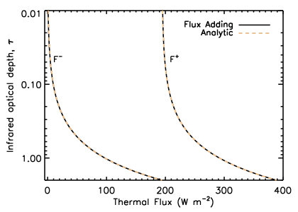
Figure 23: Layer radiative properties and thermal fluxes as a function of gray infrared optical depth from an example flux adding scenario. The atmosphere is in radiative equilibrium, is transparent to solar radiation, and thermal radiation is treated according to the gray two-stream approximation. This case has: $N=50$ atmospheric layers, a total atmospheric gray infrared optical depth $\tau^{*}=2$, and a skin temperature of 200 K. Layer transmissivities, $t_{j}$, and source terms, $s^{+,-}_{j}$, are from Equations 51 and 68, respectively. The source terms have been divided by $\sigma T_{skin}^{4}$. The source term derivatives are from Equation 69, and have been scaled by $\sigma T_{skin}^{3}$. The upwelling and downwelling fluxes, $F^{+}$ and $F^{-}$, are shown from the known analytic solution (dashed) and as computed from the flux adding approach (solid).

Figure 23 demonstrates the results of this simple example for a particular case which has: 50 atmospheric layers, a total atmospheric gray infrared optical depth $\tau^{*}=2$, and a skin temperature of 200 K. The atmospheric layers spaced in equal log units between $\tau_{0}=\tau^{*}/1000$ and the surface, which has a temperature of 288 K. The layer transmissivities decrease towards the surface as a result of the logarithmic spacing (i.e., layers near the surface are more optically thick), and the layer source terms and their derivatives increase downwards because (1) the layers have higher emissivity, and (2) temperatures are increasing towards the surface. The upwelling and downwelling thermal fluxes are in excellent agreement with the known analytic solution [e.g., 67, Equations (25) and (26)].

Appendix AA Tables and Figures

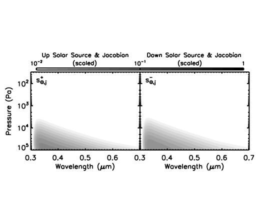
Figure 13: Initial wavelength-dependent upwelling (left) and downwelling (right) layer solar source terms (top) and their temperature derivatives (bottom) for Earth, used in our example application of the LiFE approach. Both the source terms and their derivatives have been scaled by (1) the top-of-atmosphere solar flux, which removes wavelength-dependent structure from the solar spectrum, and (2) $d\ln p_{j}$, which removes layer path length effects and creates source terms that are smooth functions of pressure. Shading is the same as Figure 9.

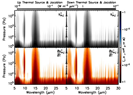
Figure 14: Initial wavelength-dependent upwelling (left) and downwelling (right) layer thermal source terms (top) and their temperature derivatives (bottom) for Earth, used in our example application of the LiFE approach. Shading is the same as Figure 10.

References

- [1] S. Manabe, R. F. Strickler, Thermal Equilibrium of the Atmosphere with a Convective Adjustment., Journal of Atmospheric Sciences 21 (1964) 361–385.
- [2] S. Manabe, R. T. Wetherald, Thermal Equilibrium of the Atmosphere with a Given Distribution of Relative Humidity., Journal of Atmospheric Sciences 24 (1967) 241–259. doi:10.1175/1520-0469(1967)024<0241:TEOTAW>2.0.CO;2.
- [3] V. Ramanathan, J. A. Coakley, Jr., Climate Modeling Through Radiative-Convective Models (Paper 8R0533), Reviews of Geophysics and Space Physics 16 (1978) 465. doi:10.1029/RG016i004p00465.
- [4] M. E. Schlesinger, J. F. B. Mitchell, Climate Model Simulations of the Equilibrium Climatic Response to Increased Carbon Dioxide (Paper 6R0726), Reviews of Geophysics 25 (1987) 760. doi:10.1029/RG025i004p00760.
- [5] J. B. Pollack, T. P. Ackerman, Possible effects of the El Chichon volcanic cloud on the radiation budget of the northern tropics, Geophys Res Lett10 (1983) 1057–1060. doi:10.1029/GL010i011p01057.
- [6] A. A. Lacis, D. J. Wuebbles, J. A. Logan, Radiative forcing of climate by changes in the vertical distribution of ozone, J Geophys Res 95 (1990) 9971–9981. doi:10.1029/JD095iD07p09971.
- [7] J. E. Hansen, L. D. Travis, Light scattering in planetary atmospheres, Space Science Reviews 16 (4) (1974) 527–610.
- [8] K. Stamnes, S.-C. Tsay, K. Jayaweera, W. Wiscombe, et al., Numerically stable algorithm for discrete-ordinate-method radiative transfer in multiple scattering and emitting layered media, Applied optics 27 (12) (1988) 2502–2509. doi:10.1364/AO.27.002502.
- [9] R. Spurr, T. Kurosu, K. Chance, A linearized discrete ordinate radiative transfer model for atmospheric remote-sensing retrieval, Journal of Quantitative Spectroscopy and Radiative Transfer 68 (6) (2001) 689–735.
- [10] R. Goody, R. West, L. Chen, D. Crisp, The correlated-k method for radiation calculations in nonhomogeneous atmospheres, Journal of Quantitative Spectroscopy and Radiative Transfer 42 (6) (1989) 539–550. doi:10.1016/0022-4073(89)90044-7.
- [11] A. A. Lacis, V. Oinas, A description of the correlated-k distribution method for modelling nongray gaseous absorption, thermal emission, and multiple scattering in vertically inhomogeneous atmospheres, J Geophys Res 96 (1991) 9027–9064. doi:10.1029/90JD01945.
- [12] J. Kiehl, B. Briegleb, A new parameterization of the absorptance due to the 15-m band system of carbon dioxide, Journal of Geophysical Research: Atmospheres (1984–2012) 96 (D5) (1991) 9013–9019.
- [13] B. P. Briegleb, Delta-eddington approximation for solar radiation in the ncar community climate model, Journal of Geophysical Research: Atmospheres (1984–2012) 97 (D7) (1992) 7603–7612.
- [14] E. J. Mlawer, S. J. Taubman, P. D. Brown, M. J. Iacono, S. A. Clough, Radiative transfer for inhomogeneous atmospheres: Rrtm, a validated correlated-k model for the longwave, Journal of Geophysical Research 102 (D14) (1997) 16663–16.
- [15] M. A. Bullock, D. H. Grinspoon, The recent evolution of climate on venus, Icarus 150 (1) (2001) 19–37.
- [16] M. J. Iacono, J. S. Delamere, E. J. Mlawer, M. W. Shephard, S. A. Clough, W. D. Collins, Radiative forcing by long-lived greenhouse gases: Calculations with the aer radiative transfer models, Journal of Geophysical Research: Atmospheres (1984–2012) 113 (D13).
- [17] R. Wordsworth, F. Forget, F. Selsis, J.-B. Madeleine, E. Millour, V. Eymet, Is gliese 581d habitable? some constraints from radiative-convective climate modeling, Astronomy and Astrophysics 522 (2010) 22.
- [18] B. P. Briegleb, Delta-Eddington approximation for solar radiation in the NCAR community climate model, J Geophys Res 97 (1992) 7603–7612. doi:10.1029/92JD00291.
- [19] E. P. Shettle, J. A. Weinman, The Transfer of Solar Irradiance Through Inhomogeneous Turbid Atmospheres Evaluated by Eddington’s Approximation., Journal of Atmospheric Sciences 27 (1970) 1048–1055. doi:10.1175/1520-0469(1970)027<1048:TTOSIT>2.0.CO;2.
- [20] D. Crisp, Radiative forcing of the Venus mesosphere. I - Solar fluxes and heating rates, Icarus 67 (1986) 484–514.
- [21] S. Chandrasekhar, Radiative Transfer, Dover, 1960.
- [22] C. D. Rodgers, Inverse Methods for Atmospheric Sounding : Theory and Practice, World Scientific, 2000.
- [23] G. L. Stephens, The transfer of radiation through vertically non uniform stratocumulus water clouds, Contributions to Atmospheric Physics 49 (4) (1976) 237–253.
- [24] M. D. Harshvardhan; King, Comparative accuracy of diffuse radiative properties computed using selected multiple scattering approximations, Journal of the Atmospheric Sciences 50 (2).
- [25] H. C. Van de Hulst, A new look at multiple scattering, NASA Institute for Space Studies, Goddard Space Flight Center, 1963.
- [26] S. Twomey, H. Jacobowitz, H. Howell, Matrix methods for multiple-scattering problems., Journal of Atmospheric Sciences 23 (1966) 289–298.
- [27] I. Grant, G. Hunt, Solution of radiative transfer problems in planetary atmospheres, Icarus 9 (1) (1968) 526–534.
- [28] J. K. Hansen, Radiative transfer by doubling very thin layers, The Astrophysical Journal 155 (1969) 565–573.
- [29] W. Wiscombe, Extension of the doubling method to inhomogeneous sources, Journal of Quantitative Spectroscopy and Radiative Transfer 16 (6) (1976) 477–489.
- [30] K. Stamnes, R. A. Swanson, A new look at the discrete ordinate method for radiative transfer calculations in anisotropically scattering atmospheres, Journal of the Atmospheric Sciences 38 (2) (1981) 387–399.
- [31] S. A. Clough, M. J. Iacono, J.-L. Moncet, Line-by-Line Calculations of Atmospheric Fluxes and Cooling Rates: Application to Water Vapor, J Geophys Res 97 (1992) 15. doi:10.1029/92JD01419.
- [32] R. J. D. Spurr, M. J. Christi, Linearization of the interaction principle: Analytic Jacobians in the “Radiant” model, J Quant Spec Rad Trans103 (2007) 431–446. doi:10.1016/j.jqsrt.2006.05.001.
- [33] V. S. Meadows, D. Crisp, Ground-based near-infrared observations of the Venus nightside: The thermal structure and water abundance near the surface, J Geophys Res 101 (1996) 4595–4622.
- [34] D. Crisp, Absorption of sunlight by water vapor in cloudy conditions: A partial explanation for the cloud absorption anomaly, Geophys Res Lett24 (1997) 571–574.
- [35] H. Savijärvi, D. Crisp, A.-M. Harri, Effects of CO2 and dust on present-day solar radiation and climate on Mars, Quarterly Journal of the Royal Meteorological Society 131 (2005) 2907–2922.
- [36] R. N. Halthore, D. Crisp, S. E. Schwartz, G. Anderson, A. Berk, B. Bonnel, O. Boucher, F.-L. Chang, M.-D. Chou, E. E. Clothiaux, et al., Intercomparison of shortwave radiative transfer codes and measurements, Journal of Geophysical Research: Atmospheres (1984–2012) 110 (D11).
- [37] T. D. Robinson, V. S. Meadows, D. Crisp, D. Deming, M. F. A’Hearn, D. Charbonneau, T. A. Livengood, S. Seager, R. K. Barry, T. Hearty, T. Hewagama, C. M. Lisse, L. A. McFadden, D. D. Wellnitz, Earth as an Extrasolar Planet: Earth Model Validation Using EPOXI Earth Observations, Astrobiology 11 (2011) 393–408.
- [38] R. A. McClatchey, R. W. Fenn, J. E. A. Selby, F. E. Volz, J. S. Garing, Optical Properties of the Atmosphere (Third Edition), Tech. rep., Air Force Cambridge Research Labs (Aug. 1972).
- [39] B. Conrath, R. Curran, R. Hanel, V. Kunde, W. Maguire, J. Pearl, J. Pirraglia, J. Welker, T. Burke, Atmospheric and surface properties of mars obtained by infrared spectroscopy on mariner 9, Journal of Geophysical Research 78 (20) (1973) 4267–4278.
- [40] B. J. Conrath, Thermal structure of the martian atmosphere during the dissipation of the dust storm of 1971, Icarus 24 (1) (1975) 36–46.
- [41] A. K. Blackadar, The vertical distribution of wind and turbulent exchange in a neutral atmosphere, Journal of Geophysical Research 67 (8) (1962) 3095–3102.
- [42] R. Haus, D. Kappel, G. Arnold, Radiative heating and cooling in the middle and lower atmosphere of Venus and responses to atmospheric and spectroscopic parameter variations, Planetary Space Sci117 (2015) 262–294. doi:10.1016/j.pss.2015.06.024.
- [43] M. Gruszka, A. Borysow, Roto-Translational Collision-Induced Absorption of CO 2for the Atmosphere of Venus at Frequencies from 0 to 250 cm -1, at Temperatures from 200 to 800 K, Icarus 129 (1997) 172–177. doi:10.1006/icar.1997.5773.
- [44] Y. I. Baranov, W. J. Lafferty, G. T. Fraser, Infrared spectrum of the continuum and dimer absorption in the vicinity of the O2 vibrational fundamental in O2/CO2 mixtures, Journal of Molecular Spectroscopy 228 (2004) 432–440. doi:10.1016/j.jms.2004.04.010.
- [45] R. Wordsworth, F. Forget, V. Eymet, Infrared collision-induced and far-line absorption in dense CO 2 atmospheres, Icarus 210 (2010) 992–997. doi:10.1016/j.icarus.2010.06.010.
- [46] Y. J. Lee, H. Sagawa, R. Haus, S. Stefani, T. Imamura, D. V. Titov, G. Piccioni, Sensitivity of net thermal flux to the abundance of trace gases in the lower atmosphere of Venus, Journal of Geophysical Research (Planets) 121 (2016) 1737–1752. doi:10.1002/2016JE005087.
- [47] L. S. Rothman, I. E. Gordon, R. J. Barber, H. Dothe, R. R. Gamache, A. Goldman, V. I. Perevalov, S. A. Tashkun, J. Tennyson, HITEMP, the high-temperature molecular spectroscopic database, J Quant Spec Rad Trans111 (2010) 2139–2150. doi:10.1016/j.jqsrt.2010.05.001.
- [48] X. Huang, R. R. Gamache, R. S. Freedman, D. W. Schwenke, T. J. Lee, Reliable infrared line lists for 13 CO2 isotopologues up to E=18,000 cm-1 and 1500 K, with line shape parameters, J Quant Spec Rad Trans147 (2014) 134–144. doi:10.1016/j.jqsrt.2014.05.015.
- [49] L. S. Rothman, I. E. Gordon, Y. Babikov, A. Barbe, D. Chris Benner, P. F. Bernath, M. Birk, L. Bizzocchi, V. Boudon, L. R. Brown, A. Campargue, K. Chance, E. A. Cohen, L. H. Coudert, V. M. Devi, B. J. Drouin, A. Fayt, J.-M. Flaud, R. R. Gamache, J. J. Harrison, J.-M. Hartmann, C. Hill, J. T. Hodges, D. Jacquemart, A. Jolly, J. Lamouroux, R. J. Le Roy, G. Li, D. A. Long, O. M. Lyulin, C. J. Mackie, S. T. Massie, S. Mikhailenko, H. S. P. Müller, O. V. Naumenko, A. V. Nikitin, J. Orphal, V. Perevalov, A. Perrin, E. R. Polovtseva, C. Richard, M. A. H. Smith, E. Starikova, K. Sung, S. Tashkun, J. Tennyson, G. C. Toon, V. G. Tyuterev, G. Wagner, The HITRAN2012 molecular spectroscopic database, J Quant Spec Rad Trans130 (2013) 4–50. doi:10.1016/j.jqsrt.2013.07.002.
- [50] V. Moroz, L. Zasova, Vira-2: A review of inputs for updating the venus international reference atmosphere, Advances in Space Research 19 (8) (1997) 1191–1201.
- [51] S. Tellmann, M. Pätzold, B. Häusler, M. K. Bird, G. L. Tyler, Structure of the venus neutral atmosphere as observed by the radio science experiment vera on venus express, Journal of Geophysical Research: Planets 114 (E9).
- [52] A. Seiff, J. T. Schofield, A. J. Kliore, F. W. Taylor, S. S. Limaye, Models of the structure of the atmosphere of Venus from the surface to 100 kilometers altitude, Advances in Space Research 5 (1985) 3–58. doi:10.1016/0273-1177(85)90197-8.
- [53] M. Tomasko, L. Doose, P. H. Smith, A. Odell, Measurements of the flux of sunlight in the atmosphere of venus, Journal of Geophysical Research 85 (A13) (1980) 8167–8186.
- [54] H. Revercomb, L. Sromovsky, V. Suomi, R. Boese, Net thermal radiation in the atmosphere of venus, Icarus 61 (3) (1985) 521–538.
- [55] D. Crisp, W. M. Sinton, K.-W. Hodapp, B. Ragent, F. Gerbault, J. H. Goebel, The nature of the near-infrared features on the Venus night side, Science 246 (1989) 506–509. doi:10.1126/science.246.4929.506.
- [56] G. Arney, V. Meadows, D. Crisp, S. J. Schmidt, J. Bailey, T. Robinson, Spatially resolved measurements of H2O, HCl, CO, OCS, SO2, cloud opacity, and acid concentration in the Venus near-infrared spectral windows, Journal of Geophysical Research (Planets) 119 (2014) 1860–1891.
- [57] D. Crisp, D. Titov, The Thermal Balance of the Venus Atmosphere, in: S. W. Bougher, D. M. Hunten, R. J. Phillips (Eds.), Venus II: Geology, Geophysics, Atmosphere, and Solar Wind Environment, 1997, p. 353.
- [58] R. Haus, D. Kappel, G. Arnold, Radiative energy balance of Venus: An approach to parameterize thermal cooling and solar heating rates, Icarus 284 (2017) 216–232. doi:10.1016/j.icarus.2016.11.025.
- [59] J. F. Kasting, Runaway and moist greenhouse atmospheres and the evolution of Earth and Venus, Icarus 74 (1988) 472–494.
- [60] J. F. Kasting, D. P. Whitmire, R. T. Reynolds, Habitable Zones around Main Sequence Stars, Icarus 101 (1993) 108–128.
- [61] R. K. Kopparapu, R. Ramirez, J. F. Kasting, V. Eymet, T. D. Robinson, S. Mahadevan, R. C. Terrien, S. Domagal-Goldman, V. Meadows, R. Deshpande, Habitable Zones around Main-sequence Stars: New Estimates, The Astrophysical Journal 765 (2013) 131. arXiv:1301.6674.
- [62] R. M. Ramirez, R. Kopparapu, M. E. Zugger, T. D. Robinson, R. Freedman, J. F. Kasting, Warming early Mars with CO2 and H2, Nature Geoscience 7 (2014) 59–63. arXiv:1405.6701, doi:10.1038/ngeo2000.
- [63] R. Wordsworth, Y. Kalugina, S. Lokshtanov, A. Vigasin, B. Ehlmann, J. Head, C. Sanders, H. Wang, Transient reducing greenhouse warming on early Mars, Geophys Res Lett44 (2017) 665–671. arXiv:1610.09697, doi:10.1002/2016GL071766.
- [64] C. Rodgers, C. Walshaw, The computation of infra-red cooling rate in planetary atmospheres, Quarterly Journal of the Royal Meteorological Society 92 (391) (1966) 67–92.
- [65] B. Armstrong, Theory of the diffusivity factor for atmospheric radiation, Journal of Quantitative Spectroscopy and Radiative Transfer 8 (9) (1968) 1577–1599.
- [66] D. G. Andrews, An introduction to atmospheric physics, Cambridge University Press, 2010.
- [67] T. D. Robinson, D. C. Catling, An analytic radiative-convective model for planetary atmospheres, The Astrophysical Journal 757 (1) (2012) 104.