Argyres-Douglas theories, Painlevé II and quantum mechanics

Abstract

We show in details that the all order genus expansion of the two-cut Hermitian cubic matrix model reproduces the perturbative expansion of the $H_{1}$ Argyres-Douglas theory coupled to the $\Omega$ background. In the self-dual limit we use the Painlevé/gauge correspondence and we show that, after summing over all instanton sectors, the two-cut cubic matrix model computes the tau function of Painlevé II without taking any double scaling limit or adding any external fields. We decode such solution within the context of trans-series. Finally in the Nekrasov-Shatashvili limit we connect the $H_{1}$ and the $H_{0}$ Argyres-Douglas theories to the quantum mechanical models with cubic and double well potentials.

1 Introduction

Argyres-Douglas (AD) theories are four dimensional ${\cal N}=2$ superconformal field theories which were first discovered at special points in the moduli spaces of 4d ${\cal N}=2$ SQCDs where mutually non-local dyons become massless simultaneously ad1 ; ad2 . Examples include the $H_{0},H_{1}$, and $H_{2}$ theories which are limits of $SU(2)$ SQCDs with $N_{f}=1,2$ and $3$ flavors respectively. Matrix model expressions for a number of AD theories have been conjectured in tc12 ; Rim:2012tf . Recently, AD theories have been studied in connection with the theory of Painlevé equations. It was first observed in Kajiwara:2004ri that the Seiberg-Witten (SW) curves of four dimensional ${\cal N}=2$ $SU(2)$ SQCDs theories can be extracted from Painlevé equations. This observation was made concrete in the breakthrough works of gil1 ; gil which established a precise correspondence between the tau functions of Painlevé VI, V, III and ${\cal N}=2$ $SU(2)$ SQCDs in the self-dual $\Omega$ background. This picture was recently further generalized in betal showing that the partition functions of the $H_{0},H_{1}$ and $H_{2}$ AD theories compute the tau functions of the Painlevé I, II and IV equations. One of the purposes of this paper is to combine these recent progress in the theory of Painlevé equations with some previous works on AD theory, matrix models and resurgence.

More precisely in section 2 we show that the all order genus expansion of the $H_{1}$ theory in the magnetic frame coupled to the $\Omega$ background is identical to the all order ’t Hooft expansion of the $\beta$ deformed cubic matrix model in the two-cut phase. In view of the Painlevé/gauge correspondence betal , we will focus on the the non-deformed case, i.e. $\beta=1$, which is defined as

$$Z(N)=\frac{1}{\text{vol}(U(N))}\int{\rm d}\Phi{\rm e}^{-\tfrac{1}{g_{s}}\mathop{\rm Tr}\nolimits W(\Phi)}\ ,$$ (1.1)

where $\Phi$ is an $N\times N$ Hermitian matrix, and the potential is

$$W(x)=\frac{m}{2}x^{2}+\frac{1}{3}x^{3}\ .$$ (1.2)

In the one-cut phase of the model all the $N$ eigenvalues of $\Phi$ condensate around the minimum $x=0$ of the potential and it is possible to show that there exists a double scaling limit of this model

$$N\to\infty,\quad t=g_{s}N\to t_{c}=\frac{m^{3}}{12\sqrt{3}}\ ,$$ (1.3)

where one reproduces the solution to the Painlevé I equation. See kkn for a simple derivation and DiFrancesco:1993cyw for a review and a list of references. In the two-cut phase instead one assumes that $N_{1}$ eigenvalues condensate around $x=0$ and $N_{2}$ eigenvalues around the other critical point of (1.2) namely $x=-m$. In this case it is possible to write the model as Cachazo:2001jy

$$Z(N_{1},N_{2})={1\over{\rm Vol}(U(N_{1}))\times{\rm Vol}(U(N_{2}))}\int D\Phi_{1}D\Phi_{2}{\rm e}^{-{1\over g_{s}}\left(W_{1}(\Phi_{1})+W_{2}(\Phi_{2})+W_{\rm int}(\Phi_{1},\Phi_{2})\right)},$$ (1.4)

where $W_{1}(\Phi_{1})$ and $W_{2}(\Phi_{2})$ are cubic potentials while $W_{\rm int}(\Phi_{1},\Phi_{2})$ is an interaction term taking into account the distribution of eigenvalues between the two critical points of the cubic potential (see equation (2.16) for the precise definition). This matrix model was studied in great details in Cachazo:2001jy ; kmt ; kmr , which we quickly review in section 2.1, as it describes topological string theory on some particular Dijkgraaf-Vafa geometry. The refinement of such topological string theory is captured by the $\beta$ deformation of the matrix model (1.4) which has been studied in detail in huangb and whose explicit expression is later given in equation (2.44). We demonstrate in detail in sections 2.2, 2.3 that such a matrix model also computes the partition function of the $H_{1}$ theory coupled to the $\Omega$ background where

$$\beta=-\epsilon_{1}/\epsilon_{2}$$ (1.5)

and we note by $\epsilon_{i}$ the $\Omega$ background regulators.

Thanks to the relation between AD theories in the self-dual background and Painlevé equations established in betal , we can then connect the cubic matrix model (1.4) to the $\tau$ function of the Painlevé II equation (PII) at long time $T\rightarrow\infty$ without taking any double scaling limit, and for generic values of the integration constants as we show in section 3. We would like to note that the two-cut phase of the quartic matrix model is known to be related to Painlevé II in a particular double scaling limit; see for instance Schiappa:2013opa ; mmnp and references therein. However in this work instead we consider the two-cut case of the cubic matrix model and we do not take any scaling limit. The $\tau$-function of PII has the following structure betal ; Its:2016jkt

$$\tau_{II}(T)\propto\sum_{n\in{\mathbb{Z}}}{{\rm e}^{{\rm i}n\rho}}{\rm e}^{{\rm i}n(2\sqrt{2}/3)T^{3/2}}{\cal G}^{\prime}(T,\nu+n)\ ,\quad T\rightarrow\infty\ ,$$ (1.6)

where $(\nu,\rho)$ are integration constants and $T$ is the time. In betal the quantity ${\cal G}^{\prime}$ is given as a series expansion in $T^{-3/2}$ and the first few terms have been computed explicitly. As explained in section 3 we find that the two-cut cubic matrix model is identified with the summand ${\cal G}^{\prime}(T,\nu)$. This observation enables us to compute ${\cal G}^{\prime}(T,\nu)$ at large $T$ up to very high orders and then to study the convergence properties of the solution proposed in betal ; Its:2016jkt . For some particular choice of integration constants we can give an all order formula for ${\cal G}^{\prime}(T,\nu)$ (see equations (3.85),(3)). We find that the long time expansion of betal ; Its:2016jkt is in fact divergent and we argue in section 4 that the summation over $n$ in (1.6) amounts to a sum over all instanton sectors in the matrix model, and that the instantons have the correct action as extracted from the analysis of the large order behaviour of ${\cal G}^{\prime}(T,\nu)$, namely

$${\rm i}\,2\sqrt{2}/3\ .$$ (1.7)

At the end of section 4 we briefly discuss Borel summability of (1.6).

Finally in section 5 we discuss the $H_{1}$ and $H_{0}$ theories in the NS phase of the $\Omega$ background and we show that these theories can be used to compute the all order WKB periods of the QM models with the cubic and the double well potentials. This provides a gauge theory justification for the holomorphic anomaly algorithm proposed in csm to determine the spectra of these QM models.

2 Matrix model and Argyres-Douglas theory

In this section, we show that perturbatively the two-cut phase of the $\beta$ deformed Hermitian cubic matrix model can be identified with the $H_{1}$ Argyres-Douglas theory in the magnetic frame coupled to the $\Omega$ background. The ’t Hooft expansion of the Hermitian cubic matrix has been discussed for instance in Cachazo:2001jy ; kmt ; kmr ; Dijkgraaf:2002pp , while its $\beta$ deformation was studied in huangb , see also Maruyoshi:2014eja ; bmt for more details on the $\beta$ deformed models. Some results for the free energies of the $H_{1}$ theory can be found for instance in Masuda:1996xj ; betal . We quickly review these two theories, and then demonstrate how they can be identified. Our derivation is rigorous for the case $\beta=1$ but it relies on some conjectural results of huangb for the case $\beta\neq 1$.

Physically, one can argue in favour of a connection between this matrix model and the $H_{1}$ theory by following tc12 ; Rim:2012tf even though the details of the connection and the precise dictionary between these two theories was not spelled out in these references. The proposal of tc12 ; Rim:2012tf was intended to give matrix model realisations for the irregular conformal blocks studied in Bonelli:2011aa ; Gaiotto:2012sf and it involves in general a Riemann sphere with an irregular singularity at infinity and a regular singularity at $z=0$. This gives a matrix model with potential

$${1\over g_{s}}V(z)=\alpha^{(0)}\log z-\sum_{k=1}^{n}{c_{k}^{(\infty)}z^{k}\over k}.$$ (2.8)

The coefficient $\alpha^{(0)}$ characterises the regular singularity at $z=0$. Then one can argue that by taking the limit $\alpha^{(0)}\to 0$ one removes the regular singularity, in which case one arrives at the $A_{2n-3}$ AD theories (only irregular singularity at infinity), to which the $H_{1}$ theory belongs. This is how one can argue for a connection between the $H_{1}$ theory and the cubic matrix model from the perspective of tc12 . Notice however that strictly speaking in the approach of tc12 removing all the regular singularities may not be completely justified, and furthermore the details of the connection and a precise dictionary was not proposed. On the other hand, even if the physical justification given above is not very rigorous, in the forthcoming section, after establishing the precise dictionary, we will verify by a direct computation that the model (1.4) computes the all order genus expansion of the $H_{1}$ theory.

2.1 The two cut phase of the cubic model

We first study in some details the case $\beta=1$ since we will need it in the forthcoming section and we briefly illustrate the case of generic $\beta$ at the end of this subsection.

We consider the hermitian matrix model

$$Z(N)=\frac{1}{\text{vol}(U(N))}\int{\rm d}M{\rm e}^{-\tfrac{1}{g_{s}}\mathop{\rm Tr}\nolimits W(M)}\ ,$$ (2.9)

where $M$ is an $N\times N$ hermitian matrix, and the potential is

$$W(x)=\frac{m}{2}x^{2}+\frac{1}{3}x^{3}\ .$$ (2.10)

This potential has two critical points at $x=0$ and $x=-m$ respectively. Let us consider the vacuum where $N_{1}$ eigenvalues of $M$ condensate at the critical point $x=0$, while $N_{2}$ eigenvalues condensate at $x=-m$, such that $N_{1}+N_{2}=N$. When expanded around this vacuum, the matrix model can be written as

$$Z(N_{1},N_{2})={1\over N_{1}!N_{2}!}\int\prod_{k=1}^{N}\frac{{\rm d}x_{k}}{2\pi}\,{\overline{\Delta}}^{2}(x){\rm e}^{-\tfrac{1}{g_{s}}{\overline{W}}(x_{k})}\ ,$$ (2.11)

where

$$\overline{\Delta}^{2}(x)=\prod_{1\leq i_{1}<i_{2}\leq N_{1}}(x_{i_{1}}-x_{i_{2}})^{2}\prod_{N_{1}+1\leq j_{1}<j_{2}\leq N}(x_{j_{1}}-x_{j_{2}})^{2}\prod_{1\leq i\leq N_{1},N_{1}+1\leq j\leq N}(x_{i}-x_{j}+m)^{2}\ ,$$ (2.12)

and

$${\overline{W}}(x_{k})=\sum_{i=1}^{N_{1}}\left(\frac{m}{2}x_{i}^{2}+\frac{1}{3}x_{i}^{3}\right)+\sum_{i=N_{1}+1}^{N}\left(-\frac{m}{2}x_{i}^{2}+\frac{1}{3}x_{i}^{3}\right)+{m^{3}\over 6}N_{2}\ .$$ (2.13)

In (2.11) we have multiplied (2.9) by

$${N!\over N_{1}!N_{2}!}$$ (2.14)

to take into account the different ways in which the eigenvalues distribute. We can view (2.11) as a two-matrix model integral kmt ; kmr ; Cachazo:2001jy ; Dijkgraaf:2002pp

$$Z(N_{1},N_{2})={1\over{\rm Vol}(U(N_{1}))\times{\rm Vol}(U(N_{2}))}\int{\rm d}\Phi_{1}{\rm d}\Phi_{2}\,{\rm e}^{-{1\over g_{s}}\left(W_{1}(\Phi_{1})+W_{2}(\Phi_{2})+W(\Phi_{1},\Phi_{2})\right)},$$ (2.15)

where $\Phi_{1},\Phi_{2}$ are $N_{1}\times N_{1}$ and $N_{2}\times N_{2}$ matrices respectively, and the potentials are

$$W_{1}(\Phi_{1})= {\rm Tr}\Bigl{(}{1\over 2}m\Phi_{1}^{2}+{1\over 3}\Phi_{1}^{3}\Bigr{)}\ ,$$ (2.16)

$$W_{2}(\Phi_{2})= -{\rm Tr}\Bigl{(}{1\over 2}m\Phi_{2}^{2}-{1\over 3}\Phi_{2}^{3}\Bigr{)}\ ,$$

$$W_{\rm int}(\Phi_{1},\Phi_{2})= N_{2}{m^{3}\over 6}+2N_{1}N_{2}\ln\left(m\right)+2\sum_{k=1}^{\infty}\frac{1}{km^{k}}\sum_{p=0}^{k}(-1)^{p}{k\choose p}{\rm tr}\,\Phi_{1}^{p}~{}{\rm tr}\,\Phi_{2}^{k-p}\ .$$

Note that for the above two-matrix model to be perturbatively well defined we have to choose $\Phi_{1}$ to be hermitian and $\Phi_{2}$ anti-hermitian. In other words, in the eigenvalue formalism (2.11), we choose

$$x_{i}=\left\{\begin{array}[]{cc}&\in{\mathbb{R}}\quad\quad i\leq N_{1}\\ &\in{\rm i}{\mathbb{R}}\quad\text{otherwise}\end{array}\right.\ .$$ (2.17)

In this section we are interested in the ’t Hooft expansion of the matrix model (2.11)

$$N_{i}\rightarrow\infty\ ,\;g_{s}\rightarrow 0\ ,\quad S_{i}=g_{s}N_{i}\;\text{fixed}\ ,\quad i=1,2\ .$$ (2.18)

We have defined the partial ’t Hooft parameters $S_{1,2}$ such that

$$S_{1}+S_{2}=t=g_{s}N\ .$$ (2.19)

In this regime the matrix model integral can be canonically expanded as

$$\log Z(N_{1},N_{2})=\sum_{g\geq 0}g_{s}^{2g-2}F_{g}(S_{1},S_{2})\ ,$$ (2.20)

where $F_{g}$ are the genus $g$ free energies.

The free energies of the matrix model can be computed from the spectral curve of the Hermitian matrix model and the associated 1-differential. The spectral curve reads

$$\mathcal{C}^{\text{mm}}:\;y^{2}=W^{\prime}(x)^{2}+f(x)=x^{2}(x+m)^{2}+\lambda x+\mu\ ,$$ (2.21)

while the associated the 1-differential is

$$\Omega^{\text{mm}}=y(x){\rm d}x\ .$$ (2.22)

The spectral curve is defined to be the deformation of the singular curve

$$y^{2}=W^{\prime}(x)^{2}\ ,$$ (2.23)

where the two singular points $a_{1},a_{2}$ ($a_{2}>a_{1}>0$) are the two critical points of the matrix model potential. After turning on the deformation $f(x)=\lambda x+\mu$, the two singular points extend to two branch cuts on the real axis, whose endpoints we denote by $a_{1}^{-},a_{1}^{+}$ and $a_{2}^{-},a_{2}^{+}$ respectively. Sometimes we denote the branch points also by

$$(a_{1}^{-},a_{1}^{+},a_{2}^{-},a_{2}^{+})\;\rightarrow\;(x_{1},x_{2},x_{3},x_{4})\ ,$$ (2.24)

from leftmost to rightmost, and the spectral curve then reads

$$y^{2}=\prod_{i=1}^{4}(x-x_{i})\ .$$ (2.25)

Let us introduce the variables

$$z_{1}=\frac{1}{4}(x_{2}-x_{1})^{2}\ ,\quad z_{2}=\frac{1}{4}(x_{4}-x_{3})^{2}\ ,$$ (2.26)

that measure the width of the branch cuts. Clearly the spectral curve is singular when $z_{1}=0$ or $z_{2}=0$. The spectral curve can also become singular when $x_{3}\rightarrow x_{2}$ so that the two branch cuts fuse into one. This is what is called the dual conifold point in the language of csm .

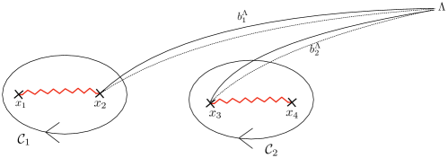
We are interested in the limits when $z_{1,2}$ are small, where the partial ’t Hooft parameters $S_{1,2}$ are locally good coordinates on the moduli space. They can be identified with the integrals of the canonical 1-form along the cycles $C_{1,2}$ that surround the branch cuts (see Fig. 1)

$$S_{i}=\frac{1}{2\pi{\rm i}}\int_{a_{i}^{-}}^{a_{i}^{+}}\Omega^{\text{mm}}\ ,\quad i=1,2\ .$$ (2.27)

Figure 1: Path of integrals in the period calculations kmr .

Performing the period integrals explicitly, one finds Cachazo:2001jy

$$S_{1}=\frac{1}{4}z_{1}\cdot I-\frac{1}{2I}K(z_{1},z_{2},I^{2})\ ,$$ (2.28)

$$S_{2}=-\frac{1}{4}z_{2}\cdot I+\frac{1}{2I}K(z_{1},z_{2},I^{2})\ .$$

Here $I$ is

$$I^{2}=\frac{1}{4}((x_{3}+x_{4})-(x_{1}+x_{2}))^{2}=m^{2}-2(z_{1}+z_{2})\ ,$$ (2.29)

and $K(z_{1},z_{2},I^{2})$ is a transcendental function symmetric in $z_{1},z_{2}$, whose expansion reads

$$K(z_{1},z_{2},I^{2})=\sum_{n,m=0}^{\infty}\frac{(n+m)\,\Gamma(2n+2m)}{2^{2n+2m+1}\Gamma(n+2)\Gamma(n+1)\Gamma(m+2)\Gamma(m+1)}\frac{z_{1}^{n+1}z_{2}^{m+1}}{(I^{2})^{m+n}}\ .$$ (2.30)

Let us introduce

$$t=S_{1}+S_{2}=\frac{1}{4}(z_{1}-z_{2})\cdot I\ ,$$ (2.31)

$$s=S_{1}-S_{2}\ .$$

Clearly the period $t$ is only an algebraic function of $z_{1},z_{2}$, and borrowing the terminology of gauge theories it can be termed a mass parameter, while $s$, being a transcendental function, is the only true modulus. In terms of the parameters $\lambda,\mu$ of the spectral curve that control the width of the branch cuts, since

$$t=S_{1}+S_{2}=-\frac{1}{2}\oint_{\infty}\frac{{\rm d}x}{2\pi{\rm i}}y(x)=\frac{\lambda}{4}\ ,$$ (2.32)

we conclude that $\lambda$ is associated to the mass parameter, while $\mu$ is associated to the true modulus $s$.

In order to compute the planar free energy $F_{0}$, we introduce the dual periods $\Pi_{i}$, which are integrals of the 1-differential along the dual cycles $b_{1,2}^{\Lambda}$ that extend from $a_{1}^{+},a_{2}^{-}$ to the UV regulation point $\Lambda$ (see Fig. 1)

$$\Pi_{i}=\int_{b_{i}^{\Lambda}}\Omega^{\text{mm}}\ ,\quad i=1,2\ .$$ (2.33)

The planar free energy in the small $z_{1,2}$ limit is determined by the special geometry relation, which reads,

$$\frac{\partial F_{0}}{\partial S_{i}}=\Pi_{i}\ ,\quad i=1,2\ ,$$ (2.34)

or if only the true modulus $s$ is used

$$\frac{\partial}{\partial s}F_{0}=\frac{1}{2}(\Pi_{1}-\Pi_{2})\ .$$ (2.35)

In addition, since

$$\frac{\partial}{\partial\mu}\Omega^{\text{mm}}={1\over 2}\frac{{\rm d}x}{y(x)}\ ,$$ (2.36)

the periods $S_{1,2},\Pi_{1,2}$ can be expressed in terms of elliptic integrals

$$2\pi{\rm i}\frac{\partial}{\partial\mu}S_{1} =-2\pi{\rm i}\frac{\partial}{\partial\mu}S_{2}={1\over 2}\int_{x_{1}}^{x_{2}}\frac{{\rm d}x}{y(x)}=-\frac{{\rm i}}{\sqrt{(x_{1}-x_{3})(x_{2}-x_{4})}}K(k^{2})\ ,$$ (2.37)

$$\frac{\partial}{\partial\mu}(\Pi_{1}-\Pi_{2}) ={1\over 2}\int_{x_{2}}^{x_{3}}\frac{{\rm d}x}{y(x)}=\frac{1}{\sqrt{(x_{1}-x_{3})(x_{2}-x_{4})}}K(k^{\prime 2})\ ,$$

with

$$k^{2}=\frac{(x_{1}-x_{2})(x_{3}-x_{4})}{(x_{1}-x_{3})(x_{2}-x_{4})}\ ,\quad k^{\prime 2}=1-k^{2}\ .$$ (2.38)

As a result, we can also write the planar free energy as

$$\partial^{2}_{s}F_{0}=-\frac{\pi}{2}\frac{K(k^{\prime 2})}{K(k^{2})}\ .$$ (2.39)

The genus one free energy $F_{1}$ can be computed using the Akemann formula for a two-cut matrix model Akemann:1996zr ; kmr

$$F_{1}=-\frac{1}{24}\sum_{i=1}^{4}\log M_{i}^{(1)}-\frac{1}{2}\log K(k^{2})-\frac{1}{12}\log\Delta+\frac{1}{8}\log(x_{1}-x_{3})^{2}+\frac{1}{8}(x_{2}-x_{4})^{2}+\text{const.}\ ,$$ (2.40)

where $\Delta$ is the discriminant

$$\Delta=\prod_{i<j}(x_{i}-x_{j})^{2}\ ,$$ (2.41)

and the moments $M_{i}^{(1)}$ are all $1$ in the cubic matrix model. Explicitly when $s,t$ are small, we have kmt

$$F_{1}=-\frac{1}{12}\log(s^{2}-t^{2})+\frac{1}{6m^{3}}s+\frac{1}{12m^{6}}(45s^{2}-17t^{2})+\frac{1}{36m^{9}}(3101s^{3}-1773st^{2})+{\mathsf{O}}(s^{3},t^{3})\ .$$ (2.42)

Note that by applying (2.37) the Akemann formula can be cast in the form (up to a constant)

$$F_{1}=-\frac{1}{2}\log\left(\frac{\partial s}{\partial\mu}\right)-\frac{1}{12}\log\Delta\ .$$ (2.43)

Finally, the free energies of higher genera can be computed by using the holomorphic anomaly equations bcov as demonstrated in kmr . It requires as initial data the flat coordinates, $s$ and $t$, the planar and genus one free energies in the small $z_{1,2}$ limit, as well as the transformation of these local data to the vicinity of the conifold singularity. In turns these quantities are determined by the spectral curve and the the choice of 1-differential. The higher genera free energies of the hermitian matrix model could also be computed by the means of topological recursion eo , using the spectral curve (2.21) and the 1-differential (2.22).

Let us now briefly discuss the $\beta$ deformation of the cubic model namely huangb

$$Z_{\beta}(N_{1},N_{2})={1\over N_{1}!N_{2}!}\int\prod_{k=1}^{N}\frac{{\rm d}x_{k}}{2\pi}\,{\overline{\Delta}}^{2\beta}(x){\rm e}^{-\tfrac{\beta}{g_{s}}{\overline{W}}(x_{k})}\ .$$ (2.44)

In the t’ Hooft regime (2.18) one has

$$\log Z_{\beta}(N_{1},N_{2})=\sum_{g,n\geq 0}g_{s}^{2(g+n)-2}(-\beta)^{1-g-2n}(\beta-1)^{2n}F_{g,n}(S_{1},S_{2})\ .$$ (2.45)

When $\beta=1$ we recover (2.20) with the identification

$$F_{g,0}=F_{g}.$$ (2.46)

It was conjectured and tested in huangb that $F_{g,n}$ can be computed recursively by solving the refined holomorphic anomaly equations hk ; kwal . The latter are extension of the holomorphic anomaly equations bcov and their solution requires an additional piece of initial condition, namely the knowledge of $F_{0,1}$: the genus one free energy in the NS limit. For the matrix model (2.44) it was conjectured and tested in huangb that $F_{0,1}$ is given by

$$F_{0,1}=-\frac{1}{24}\log\Delta\ ,$$ (2.47)

where $\Delta$ is the discriminant (2.41). To our knowledge a rigorous derivation of this statement in matrix models is missing.

2.2 The $H_{1}$ Argyres-Douglas theory

We quickly review the computational aspect of the Argyres-Douglas theory called $H_{1}$ which lies inside the moduli space of ${\cal N}=2$ $SU(2)$ SQCD with two flavour $N_{f}=2$ ad2 . Just like the Seiberg-Witten theory, the $H_{1}$ theory is completely encoded in the spectral curve which is given by (we follow the notation of betal )

$$\mathcal{C}^{H_{1}}:\ y_{\rm H_{1}}^{2}=x^{4}+4cx^{2}+2{m_{\rm H_{1}}}x+{u}\ ,$$ (2.48)

as well as the associated canonical one-form

$$\Omega_{H_{1}}=y_{H_{1}}(x){\rm d}x\ .$$ (2.49)

The parameter $m_{\rm H_{1}}$ is the mass parameter, ${c}$ is the deformation parameter away from the conformal point, while ${u}$ is the Coulomb modulus. Let $e_{i}$ be the four roots of (2.48). The spectral curve can be written as

$$y_{\rm H_{1}}^{2}=\prod_{i=1}^{4}(x-e_{i})\ ,$$ (2.50)

and we introduce the periods of the 1-form (we follow the notation of Masuda:1996xj )

$$a=\int_{e_{2}}^{e_{3}}y_{\rm H_{1}}(x){\rm d}x\ ,\quad\quad a_{D}=\frac{1}{2\pi{\rm i}}\int_{e_{1}}^{e_{3}}y_{\rm H_{1}}(x){\rm d}x\ .$$ (2.51)

On the other hand, the Coulomb branch is also parameterized by the mass parameter $m_{\rm H_{1}}$, which is given by the residue of the canonical 1-form at the infinity of the $x$-plane. We choose to treat $m_{\rm H_{1}}$ in a symmetric way. For this purpose, we introduce

$${\overline{a}_{D}}={1\over 2\pi{\rm i}}\int_{e_{4}}^{e_{2}}y_{\rm H_{1}}(x){\rm d}x\ ,$$ (2.52)

which satisfies

$${a}_{D}-\overline{a}_{D}=m_{\rm H_{1}}/2\ .$$ (2.53)

It is then also convenient to introduce

$$\tilde{a}_{D}=a_{D}+\overline{a}_{D}=2a_{D}-m_{\rm H_{1}}/2\ .$$ (2.54)

In particular in the massless limit $m_{\rm H_{1}}=0$, one finds that

$$a_{D}=\overline{a}_{D}=\tilde{a}_{D}/2\ .$$ (2.55)

The singularities of the Coulomb branch are given by the zeros of the discriminant of the spectral curve

$$\Delta=256u^{3}-2048c^{2}u^{2}+4096c^{4}u+2304m_{\rm H_{1}}^{2}cu-432m_{\rm H_{1}}^{4}-1024m_{\rm H_{1}}^{2}c^{3}\ .$$ (2.56)

One reads off three singular points (perturbatively in small $m_{\rm H_{1}}$)

$$u^{(1)} =\frac{m_{\rm H_{1}}^{2}}{4c}+{\mathsf{O}}(m_{\rm H_{1}}^{4})\ ,$$ (2.57)

$$u^{(2)} =4c^{2}+2\sqrt{2}{\rm i}m_{\rm H_{1}}c^{1/2}-\frac{m_{\rm H_{1}}^{2}}{8c}+\frac{{\rm i}m_{\rm H_{1}}^{3}}{64\sqrt{2}c^{5/2}}+{\mathsf{O}}(m_{\rm H_{1}}^{4})\ ,$$

$$u^{(3)} =4c^{2}-2\sqrt{2}{\rm i}m_{\rm H_{1}}c^{1/2}-\frac{m_{\rm H_{1}}^{2}}{8c}-\frac{{\rm i}m_{\rm H_{1}}^{3}}{64\sqrt{2}c^{5/2}}+{\mathsf{O}}(m_{\rm H_{1}}^{4})\ .$$

We refer to $u^{(1)}$ as the electric point while $u^{(2)}$ and $u^{(3)}$ correspond to the magnetic and dyonic points.

In this section we focus on the magnetic frame, and consider the $H_{1}$ theory coupled to the $\Omega$ background n ; Nekrasov:2003rj where the two $\Omega$ regulators are

$$\epsilon_{1},~{}\epsilon_{2}\ .$$ (2.58)

In the magnetic frame, the good local coordinate is the period $a_{D}$, and the partition function enjoys the genus expansion

$$\log Z^{\rm D}(a_{D})=F^{\rm D}(a_{D})=\sum_{g,n\geq 0}F_{g,n}^{(D)}(a_{D})(\epsilon_{1}\epsilon_{2})^{g-1}(\epsilon_{1}+\epsilon_{2})^{2n}\ .$$ (2.59)

When $\epsilon_{1}=-\epsilon_{2}=\epsilon$ we note

$$F_{g,0}^{(D)}=F_{g}^{(D)}\ .$$ (2.60)

The prepotential $F_{0}^{(D)}$ in the magnetic frame is then determined by the following special geometry relation

$$\frac{\partial}{\partial\tilde{a}_{D}}F_{0}^{(D)}=\frac{a}{2}\ .$$ (2.61)

The genus one free energies of the gauge theory are given by Huang:2006si ; Huang:2009md

$$F^{(D)}_{1}=-\frac{1}{2}\log\left(\frac{{\rm d}\tilde{a}_{D}}{{\rm d}u}\right)-\frac{1}{12}\log\Delta\ ,$$ (2.62)

and

$$F^{(D)}_{0,1}=-\frac{1}{24}\log\Delta\ ,$$ (2.63)

Finally the higher genus free energies $F_{g,n}^{(D)}$ can also be determined by using the refined holomorphic anomaly equations Huang:2006si ; Huang:2009md ; hk ; kwal .

2.3 Identifying gauge theory with matrix model

In this section we show that the all order ’t Hooft expansion of the matrix model (2.45) is identical to the all order genus expansion of the AD theory $H_{1}$ (2.59) in the $\Omega$ background. To start with we would like to identify the spectral curves and the choices of canonical one form. After taking the shift of variables

$$x\mapsto x-m/2\ ,$$ (2.64)

the spectral curve (2.21) of the matrix model becomes

$$y^{2}=x^{4}-\frac{m^{2}}{2}x^{2}+\lambda x+\left(\frac{m^{4}}{16}-\frac{\lambda m}{2}+\mu\right)\ ,$$ (2.65)

while the associated 1-differential remains the same. It is then easy to see that both the spectral curve and the canonical differential of the cubic matrix model can be identified with those of the $H_{1}$ theory, i.e. (2.48) and (2.49), provided we use the following dictionary

$$c =-\frac{m^{2}}{8}\ ,$$ (2.66)

$$m_{\rm H_{1}} =\frac{\lambda}{2}=2t\ ,$$

$$u =\frac{m^{4}}{16}-\frac{\lambda m}{2}+\mu\ .$$

In particular, the mass parameter ${m_{\rm H_{1}}}$ and the Coulomb modulus ${u}$ of the $H_{1}$ theory are identified correspondingly with the mass parameter $\lambda\propto t$ and the true modulus $\mu$ (up to a shift) of the matrix model. Therefore, the Coulomb branch of the $H_{1}$ theory can be identified with the complexified moduli space of the cubic matrix model: both of them have the same singular points and the same metric.

Let us make the identification of singularities more explicit. We first demonstrate that the singularity of the matrix model $z_{1}\rightarrow 0$ or $z_{2}\rightarrow 0$ should be identified with $u^{(2)}$ or $u^{(3)}$ singularities of the $H_{1}$ theory. Indeed, the two singularities of the $H_{1}$ theory are related to each other by mapping

$$m_{\rm H_{1}}\rightarrow-m_{\rm H_{1}}$$ (2.67)

while keeping ${c}$ and ${u}$ fixed. On the matrix model side, if we send $t\to-t$ and keep the combinations $m^{2}$ and $m^{4}-8\lambda m+16\mu$ unchanged (c.f. (2.66)), the four branch points are mapped to

$$(x_{1},x_{2},x_{3},x_{4})\longmapsto(-x_{4},-x_{3},-x_{2},-x_{1})\ ,$$ (2.68)

which means that we merely exchange $z_{1}$ and $z_{2}$. Furthermore, let us take the simple limit $m_{\rm H_{1}}=0$, and consider the domain

$${c}<0\ ,\quad 4{c}^{2}-u>0\ ,$$ (2.69)

where the four branch points of the spectral curve of the $H_{1}$ theory lie on the real axis. It is easy then to compute the position of the four branch points and check that the confluent singularity $u^{(2)}=u^{(3)}$ of the $H_{1}$ theory corresponds to the limit $z_{1}=z_{2}=0$ of the matrix model. In addition, a simple calculation in this limit shows that the $u^{(1)}$ singularity of the $H_{1}$ theory corresponds to the dual conifold point of the matrix model, where $x_{2}=x_{3}$, and two branch cuts fuse into one. To summarize, we have the following correspondence of singular points

$$\begin{array}[]{rcl}z_{1}=0&\longleftrightarrow&u^{(2)}\\ z_{2}=0&\longleftrightarrow&u^{(3)}\\ \text{dual conifold}&\longleftrightarrow&u^{(1)}\ ,\end{array}$$ (2.70)

where we borrow the terminology of csm to denote the $u^{(1)}$ singularity. In particular the small branch cut limit $S_{1}\rightarrow 0$ indeed corresponds to the magnetic point where $a_{D}$ is small.

Given that the spectral curve and the one form in the two theories are identified, it follows that also the periods coincide. It is straightforward to check for instance that the following dictionary can be established

$$S_{1}=a_{D}$$ (2.71)

provided we identify

$$(e_{1},e_{2},e_{3},e_{4})\leftrightarrow(\tilde{x_{1}},\tilde{x}_{3},\tilde{x}_{2},\tilde{x}_{4})\ ,$$ (2.72)

where we denote the four branch points of the spectral curve after the shift (2.64) by $\tilde{x}_{i}$ ($i=1,2,3,4$). More precisely we identify

$$\begin{gathered}a_{D}=S_{1}\ ,\quad\overline{a}_{D}=-S_{2}\ ,\\ \tilde{a}_{D}=s\ ,\\ a=\Pi_{1}-\Pi_{2}\ .\end{gathered}$$ (2.73)

Consequently, in the magnetic (dyon) frame of the $H_{1}$ theory and the small $z_{1},z_{2}$ limit of the matrix model, we could identified the planar and genus one free energies of the two theories by comparing (2.61), (2.63), (2.62) and (2.35), (2.43),(2.47). Higher genera free energies can also be identified since they can be computed by using the refined holomorphic anomaly equations on both sides.

In fact, at least for the case $\beta=1$, as long as we make the conjecture that the $H_{1}$ theory has an underlying hermitian matrix model so that the topological recursion eo is applicable, the identification of spectral curve and canonical 1-form with the cubic matrix model through (2.66) already suffices to guarantee the all genus expansion of the partition functions of the two theories are in agreement.

A final note is that the spectral curve of the two-cut solution to the cubic matrix model in the $S_{1}=-S_{2}$ slice itself can be identified with many other theories, like the pure $SU(2)$. But since their 1-forms are different, not all their free energies can be identified. The case of pure $SU(2)$ is discussed in kmt ; kmr , where it is pointed out that one only has the agreement of $\partial^{2}F_{0}$ and $F_{1}$.

3 The two-cut model and the Painlevé/gauge correspondence

We provide here a concrete link between the two-cut matrix model (2.15) and the proposal of betal where the partition function of the $H_{1}$ theory was computed in the large $c$ regime (2.48).

We consider the limit

$$g_{s}\rightarrow 0\ ,\quad N_{1},N_{2}\;\;\text{finite}\ ,$$ (3.74)

in which case, the matrix integral has the decomposition

$$Z_{\text{mm}}(N_{1},N_{2})=Z_{\text{mm}}^{\text{np}}(N_{1},N_{2})\left(1+\sum_{k=1}^{\infty}g_{s}^{k}Z_{\text{mm}}^{(k)}(N_{1},N_{2})\right)\ .$$ (3.75)

In order to see how the nonperturbative contributions $Z_{\text{mm}}^{\text{np}}(N_{1},N_{2})$ and perturbative contributions $Z_{\text{mm}}^{(k)}(N_{1},N_{2})$ are related to the free energies $F_{g}(t)$ of the ’t Hooft expansion, notice that the latter have the following asymptotic behavior

$$F_{0}(t) =\frac{t^{2}}{2}(\log t-1/2)+c^{(0)}_{1}t+c^{(0)}_{2}t^{2}+{\cal O}(t^{3})$$ (3.76)

$$F_{1}(t) =-\frac{1}{12}\log t+c^{(1)}_{1}t+{\cal O}(t^{2})\ ,$$

$$F_{g}(t) =\frac{B_{2g}}{2g(2g-2)t^{2g-2}}+c^{(g)}_{1}t+{\cal O}(t^{2})\ ,\quad g\geq 2\ ,$$

where for simplicity we take a one-cut matrix model as an example. Plug in $t=g_{s}N$ and take the limit (3.74), one finds

$$Z_{\text{mm}}(N)=\exp\left(\sum_{g=0}^{\infty}g_{s}^{2g-2}F_{g}(t)\right)$$

$$= \exp\left(\frac{N^{2}}{2}\left(\log(g_{s}N)-1/2\right)+\frac{c^{(0)}_{1}N}{g_{s}}+c^{(0)}_{2}N^{2}-\frac{1}{12}\log(g_{s}N)+\sum_{g=2}^{\infty}\frac{B_{2g}}{2g(2g-2)N^{2g-2}}\right)\times$$

$$\exp\left(\sum_{g=0}^{\infty}\sideset{}{{}^{\prime}}{\sum}_{n=1}^{\infty}g_{s}^{2g-2+n}c^{(g)}_{n}N^{n}\right)\ ,$$ (3.77)

where in the last line $\sideset{}{{}^{\prime}}{\sum}$ means $n$ starts from 3 if $g=0$ so that one always has $2g-2+n\geq 1$. Obviously, the second line in (3) is $Z_{\text{mm}}^{\text{np}}(N)$, and other than the ambiguous contributions $c^{(0)}_{1},c^{(0)}_{2}$ this term is universal. The third line expands to $Z_{\text{mm}}^{(k)}(N)$, and they receive leading contributions of higher genera free energies $F_{g}(t)$. Therefore the limit (3.74) gives us a means to compare more directly higher genera free energies of the two theories.

Let us come back to the two-cut solution to the cubic matrix model. The perturbative contributions have been computed in kmt up to order 6. The first few orders are kmt

$$Z_{\text{mm}}^{(1)}(N_{1},N_{2})= \frac{1}{6m^{3}}\left(2(2N_{1}^{3}-15N_{1}^{2}N_{2}+15N_{1}N_{2}^{2}-2N_{2}^{3})+(N_{1}-N_{2})\right)\ ,$$ (3.78)

$$Z_{\text{mm}}^{(2)}(N_{1},N_{2})= \frac{1}{3m^{6}}\left((8N_{1}^{4}-91N_{1}^{3}N_{2}+59N_{1}^{2}N_{2}^{2}-91N_{1}N_{2}^{3}+8N_{2}^{4})+(7N_{1}^{2}-31N_{1}N_{2}+7N_{2}^{2})\right)\ .$$ (3.79)

The nonperturbative contribution is kmt

$$Z_{\text{mm}}^{\text{np}}(N_{1},N_{2})=Z_{\text{mm}}^{\text{np,norm}}(N_{1},N_{2})Z_{\text{mm}}^{\text{np,relevant}}(N_{1},N_{2})\ ,$$ (3.80)

with

$$Z_{\text{mm}}^{\text{np,norm}}(N_{1},N_{2})={\rm i}^{N_{2}}(-1)^{\lfloor\frac{{N_{2}}}{2}\rfloor}\left(\frac{g_{s}}{m}\right)^{(N_{1}^{2}+N_{2}^{2})/2}m^{2N_{1}N_{2}}\exp\left(-\frac{m^{3}N_{2}}{6g_{s}}\right)\ ,$$ (3.81)

and

$$Z_{\text{mm}}^{\text{np,relevant}}(N_{1},N_{2})=(2\pi)^{-(N_{1}+N_{2})/2}G(1+N_{1})G(1+N_{2})\ .$$ (3.82)

Here $G(1+N)$ is the Barnes function. It vanishes when $N=-1,-2,\ldots$, and it has the following asymptotic expansion if $|N|$ is large and $N\not\in{\mathbb{R}}_{-}$

$$\log(2\pi)^{-N/2}G(1+N)=\zeta^{\prime}(-1)+\left(\frac{N^{2}}{2}-\frac{1}{12}\right)\log N-\frac{3N^{2}}{4}+\sum_{g=2}^{\infty}\frac{B_{2g}}{2g(2g-2)N^{2g-2}}\ .$$ (3.83)

In the above expression of $Z_{\text{mm}}^{\text{np}}(N_{1},N_{2})$, the factors in $Z_{\text{mm}}^{\text{np,norm}}$ contribute (up to a constant) in the ’t Hooft expansion to the ambiguous linear or quadratic terms of the planar free energy. Important are the factors in $Z_{\text{mm}}^{\text{np,relevant}}$, which are universal, and which come from volumes of the unitary groups $U(N_{1}),U(N_{2})$.

Let us turn to the gauge theory side. It has been proposed in Kajiwara:2004ri ; betal that the $H_{1}$ theory could be related to the Painlevé II equation. To be precise it was found in betal that the $\tau$-solution to the Painlevé II equation has the form

$$\tau_{II}(T)=S^{-\tfrac{1}{6}+\tfrac{\theta^{2}}{3}}\sum_{n\in{\mathbb{Z}}}{\rm e}^{{\rm i}n\rho}{\cal G}(S,\nu+n,\theta)\ ,\quad 8T^{3}=9S^{2}\ ,$$ (3.84)

where $T$ is the time, $\theta$ a parameter characterising the equation (see equation (4.101)) and $\nu,\rho$ integration constants. The summand ${\cal G}(S,\nu,\theta)$ has the decomposition

$${\cal G}(S,\nu,\theta)={{C}}(S,\nu,\theta)\left(1+\sum_{k=1}^{\infty}\frac{D_{k}(\nu,\theta)}{S^{k}}\right)\ .$$ (3.85)

The claim betal is then that, with the dictionary

$$\nu= -\sqrt{2}\,{\rm i}\,\tilde{a}_{D}/\epsilon$$ (3.86)

$$S= -{{32}\over 3}(-c)^{3/2}/\epsilon$$

$$\theta= \pm\sqrt{2}\,{\rm i}\,m_{\rm H_{1}}/\epsilon\ ,$$

the summand ${\cal G}(S,\nu,\theta)$ is identified with the partition function $Z_{\rm H_{1}}(\tilde{a}_{D},m_{\rm H_{1}},c)$ of the $H_{1}$ theory in the magnetic frame coupled to the self-dual $\Omega$ background. Note due to the gauge–matrix-model dictionary (2.73) $\tilde{a}_{D},m_{\rm H_{1}}$ can identified with the ’t Hooft parameters, and $\epsilon$ proportional to $g_{s}$, therefore we should regard $\nu,\theta$ as counterparts of the ranks $N_{1},N_{2}$ according the dictionary (3.86), and (3.85) is to be compared with the finite $N$ limit (3.74) of the matrix model.

The factor $C(S,\nu,\theta)$ is given in betal

$${{C}}(S,\nu,\theta)=(2\pi)^{-\nu}G\left(1+\nu+\frac{\theta}{2}\right)G\left(1+\nu-\frac{\theta}{2}\right)\cdot{\rm e}^{{\rm i}\nu S+\pi{\rm i}\nu^{2}/2}S^{-(\nu^{2}+\theta^{2}/4)+1/6}6^{-\nu^{2}}\ .$$ (3.87)

From the point of view of identification with the $H_{1}$ theory, the last three terms are irrelevant since they contribute to linear or quadratic terms of the planar free energy and constant term of the genus one free energy, which are ambiguous. Therefore as in the matrix model we could split $C(S,\nu,\theta)$ by

$$C(S,\nu,\theta)=C^{\text{norm}}(S,\nu,\theta)C^{\text{relevant}}(S,\nu,\theta)\ ,$$ (3.88)

where the essential part reads

$$C^{\text{relevant}}(S,\nu,\theta)=(2\pi)^{-\nu}G\left(1+\nu+\frac{\theta}{2}\right)G\left(1+\nu-\frac{\theta}{2}\right),$$ (3.89)

while the rest is collected in $C^{\text{norm}}(S,\nu,\theta)$

$$C^{\text{norm}}(S,\nu,\theta)={\rm e}^{{\rm i}\nu S+\pi{\rm i}\nu^{2}/2}S^{-(\nu^{2}+\theta^{2}/4)+1/6}6^{-\nu^{2}}\ .$$ (3.90)

The coefficients $D_{k}(\nu,\theta)$ can be in principle computed recursively. It is however hard to compute them for higher values of $k$. The first two terms are given in betal and they read

$$D_{1}({\nu},\theta)= -\frac{{\rm i}}{36}\nu\left(68\nu^{2}-9\theta^{2}+2\right)\ ,$$ (3.91)

$$D_{2}({\nu},\theta)= -\frac{289}{162}\nu^{6}+\frac{153\theta^{2}-1159}{324}\nu^{4}-\frac{81\theta^{4}-1584\theta^{2}+1084}{2592}\nu^{2}-\frac{\theta^{2}\left(11\theta^{2}-68\right)}{1728}\ .$$

Note that since very few $D_{k}(\nu,\theta)$ were computed in betal , the convergence properties of the large $S$ expansion in (3.85) could not be analysed.

One can now easily check that using the dictionary

$$S =-{\rm i}m^{3}/(6g_{s})\ ,$$ (3.92)

$$\nu =(N_{1}-N_{2})/2\ ,$$

$$\theta =-(N_{1}+N_{2})\ ,$$

the perturbative contributions of the matrix model $g_{s}^{k}Z^{(k)}_{\text{mm}}(N_{1},N_{2})$ are identified with those of the $H_{1}$ theory $S^{-k}D_{k}(\nu,\theta)$, at least for $k=1,2$, while the essential parts of the non-perturbative contributions, namely (3.89) and (3.82), agree if one replace $N_{2}$ with $-N_{2}$ in (3.82) . Hence we will use the notation

$$Z_{\text{mm}}(N_{1},N_{2})\fallingdotseq{\cal G}(S,\nu,\theta)$$ (3.94)

where $\fallingdotseq$ means that the equality is only up to the terms that become ambiguous in the ’t Hooft expansion (namely (3.81) and (3.90)) and provide we take into account the switch $N_{2}\to-N_{2}$ in (3.82). Note that the three dictionaries (2.66), (3.86), (3.92) are consistent if we choose the scaling

$$\epsilon=-2\sqrt{2}\,{\rm i}\,g_{s}\ .$$ (3.95)

Furthermore, assuming the dictionary (3.92) is correct, we can reverse the logic and use the matrix model calculation, which is much easier, to predict $D_{k}(\nu,\theta)$ for higher $k$. For instance

$$D_{3}(\nu,\theta)= \frac{{\rm i}\left(3360-28504\theta^{2}+4270\theta^{4}-99\theta^{6}\right)\nu}{62208}+\frac{{\rm i}\left(899576-700884\theta^{2}+45648\theta^{4}-729\theta^{6}\right)\nu^{3}}{279936}$$

$$+\frac{{\rm i}\left(279464-47178\theta^{2}+1377\theta^{4}\right)\nu^{5}}{23328}+\frac{{\rm i}\,17\left(2284-153\theta^{2}\right)\nu^{7}}{5832}+\frac{{\rm i}\,4913\nu^{9}}{4374}\ .$$ (3.96)

We have computed the expressions of $D_{4},D_{5},D_{6},D_{7}$ and $D_{8}$. We listed some of them in Appendix A, while the others are available upon request.

Finally, since many $D_{k}$ can be computed with relative ease, we can now analyse the convergence property of ${\cal G}(S,\nu,\theta)\propto Z_{\text{mm}}(N_{1},N_{2})$. In the cases of $(N_{1},N_{2})=(1,0),(2,0),(1,1)$, which correspond to $(\nu,\theta)=(1/2,1),(1,2),(0,2)$, $Z_{\text{mm}}(N_{1},N_{2})$ can be analytically computed,

$$Z(1,0)= {1\over 2\pi}\sum_{n=0}^{\infty}\frac{2^{3n+\tfrac{1}{2}}}{3^{2n}}\frac{g_{s}^{n+\tfrac{1}{2}}}{m^{3n+\tfrac{1}{2}}}\frac{\Gamma(3n+\tfrac{1}{2})}{(2n)!}\ ,$$

$$Z(2,0)= {1\over 2\pi}\frac{g_{s}^{2}}{m^{2}}+{1\over(2\pi)^{2}}\sum_{n=0}^{\infty}\frac{2^{3n+5}}{3^{2n+2}}\frac{g_{s}^{n+3}}{m^{3n+5}}\cdot\left(\frac{\sqrt{\pi}}{2}\frac{\Gamma(3n+\tfrac{7}{2})}{(2(n+1))!}+\sum_{k=0}^{n}\frac{\Gamma(3k+\tfrac{1}{2})\Gamma(3n-3k+\tfrac{5}{2})}{4(2k+1)!(2n-2k+2)!}\right.$$

$$\left.\phantom{\frac{\Gamma(3n+\tfrac{7}{2})}{(2(n+1))!}}\times(2k+1)(72k^{2}-6(17+18n)k+29+66n+36n^{2})\right)\ ,$$

$$Z(1,1)= {{\rm e}^{m^{2}/6}{\rm i}\over 2\pi^{2}}\left(2\pi mg_{s}+\sum_{n=2}^{\infty}\frac{2^{3n+1}}{3^{2n}}\frac{g_{s}^{n+1}}{m^{3n-1}}\left(\frac{(-1)^{n+1}15\sqrt{\pi}(n-1)(2n-1)\Gamma(3n-\tfrac{5}{2})}{8\Gamma(2n+1)}\right.\right.$$

$$\phantom{222222}+\sum_{k=0}^{n-2}\frac{(-1)^{k}9}{64(2k)!(2n-2k)!}\Gamma(3k+\tfrac{1}{2})\Gamma(3n-3k-\tfrac{11}{2})(6n-6k-5)(6n-6k-11)$$

$$\left.\left.\phantom{22222\frac{\Gamma(\tfrac{1}{2})}{\Gamma{2}}}\times(2n-2k-1)(2n-2k-3)(36k^{2}+(12-36n)k+7-12n)\right)\right)\ .$$ (3.97)

At the level of the $D_{k}$ coefficients this gives

$$D_{n}(\tfrac{1}{2},-1) =\frac{(-{\rm i})^{n}}{2^{4n}3^{3n}}\frac{(6n)!}{(3n)!(2n)!}\ ,$$

$$D_{n}(1,-2) =\frac{(-{\rm i})^{n}}{2^{4n}3^{3n}}\cdot\left(\frac{(6n)!}{(3n)!(2n)!}+2\sum_{k=0}^{n-1}\frac{(6k)!}{(3k)!(2k)!}\frac{(6n-6k-2)!}{(3n-3k-1)!(2n-2k)!}\right.$$

$$\left.\phantom{\frac{(6n-6k-2)!}{(3n-3k-1)!(2n-2k)!}}\times(72k^{2}-6(18n-1)k+36n^{2}-6n-1)\right)$$

$$D_{n}(0,-2) =\frac{(-{\rm i})^{n}}{2^{4n}3^{3n}}\cdot\left((-1)^{n+1}120\frac{(6n-6)!}{(2n)!(3n-3)!}(n-1)(2n-1)\right.$$

$$+576\sum_{k=0}^{n-2}(-1)^{k}\frac{(6k)!}{(3k)!(2k)!}\frac{(6n-6k-1)!}{(3n-3k-6)!(2n-2k)!}(6n-6k-5)$$

$$\left.\phantom{\frac{(6k)!}{(3k)!(2k)!}}\times(2n-2k-1)(2n-2k-3)(36k^{2}-(36n-12)k-12n+7)\right)\ .$$ (3.98)

All three series in (3) are divergent. In fact the coefficients of $g_{s}^{n}/m^{3n}$, denoted by $a_{n}$, in all three series have the asymptotic behavior

$$|a_{n}|\sim 6^{n}n!\ ,\quad n\rightarrow\infty\ .$$ (3.99)

We conjecture this to be always the case for any values of $N_{1},N_{2}$. As a result, $D_{n}(\nu,\theta)$ for any value of $\nu,\theta$ has the asymptotic behavior

$$D_{n}(\nu,\theta)\sim(-{\rm i})^{n}\,n!\ ,\quad n\rightarrow\infty\ .$$ (3.100)

Hence, unlike the series expansions appearing in the short time solution of Painlevé equations gil ; ilt ; gil1 , those at long time betal ; Its:2016jkt seems to suffer from divergence problems. This is somehow expected since generically also the classical special functions have divergent long-distance expansion. We will see in the next section that the sum over all integer shifts in the $\tau$ function (3.84) can be interpreted as summing over all instanton sectors and that the overall normalisation factor (3.90) leads to the correct instanton action as extracted from the analysis of the large order behaviour namely (3.100).

4 Trans-series solution to Painlevé II equation

Eq. (3.85) is given in betal as the $\tau$-function solution to the Painlevé II equation. The Painlevé II equation reads

$$q^{\prime\prime}=2q^{3}+Tq+{1\over 2}-\theta\ ,$$ (4.101)

where the derivatives of $q$ are w.r.t. $T$ while $\theta$ is a parameter. This is a second order differential equation and its solution depends on two integration constants which, by following the notation of Its:2016jkt ; betal , we denote by

$$(\nu,\rho)\ .$$ (4.102)

The corresponding $\tau$ function is defined by betal

$${{\rm d}\over{\rm d}T}\log\tau=\frac{1}{2}q^{\prime 2}+\theta q-\frac{1}{2}q^{4}-\frac{1}{2}Tq^{2}-\frac{T^{2}}{8}\ .$$ (4.103)

In Its:2016jkt ; betal it was found that the $\tau$ function associated to a generic solution to the Painlevé II equation in the large $T$ limit along the rays ${\rm arg}(T)=0,\pm{2\pi\over 3}$ can be written as

$$\tau(T,\nu,\rho,\theta)=\sum_{n\in{\mathbb{Z}}}{\rm e}^{{\rm i}n\rho}{\cal G}(S,\nu+n,\theta)\ ,$$ (4.104)

where ${\cal G}(S,\nu,\theta)$ is given in (3.85) and we use the change of variables

$$8T^{3}=9S^{2}\ .$$ (4.105)

In this section we argue that (4.104) can be reproduced by a trans-series solution to the Painlevé II equation. We will check this explicitly along the slice

$$\nu=-\theta/2\ ,$$ (4.106)

where the trans-series solution can be easily constructed by following mmnp . Let us make the following trans-series ansatz for the function $q(T)$

$$q(T,\sigma,\theta)=\sum_{n\geq 0}\sigma^{n}{\rm e}^{-nA/x}q^{(n)}(T)=x^{-1/3}\sum_{n\geq 0}\sigma^{n}{\rm e}^{-nA/x}x^{n\beta}\sum_{g\geq 0}u_{g}^{n}x^{g}\ ,$$ (4.107)

where

$$x=T^{-3/2},\quad\beta=1-{\theta},\quad A=-{2\sqrt{2}\over 3}\,{\rm i}\ .$$ (4.108)

Here $q^{(0)}(T)$ is the perturbative sector, $q^{(n\geq 1)}(T)$ different instanton sectors, and $A$ is interpreted as the instanton action. By plugging this ansatz in (4.101) we can compute all the coefficients. We find for instance for the perturbative part

$$u_{0}^{0}=-\frac{{\rm i}}{\sqrt{2}},\quad u_{1}^{0}=\frac{1}{4}-\frac{\theta}{2},\quad u_{2}^{0}=-\frac{{\rm i}(12(\theta-1)\theta+5)}{16\sqrt{2}},\quad\cdots$$ (4.109)

and the first instanton sector

$$u_{1}^{1}= -\frac{{\rm i}(3\theta(7\theta-10)+14)}{12\sqrt{2}}u_{0}^{1}\ ,$$ (4.110)

$$u_{2}^{1}= \frac{1}{576}(3\theta(\theta(3(222-49\theta)\theta-1045)+844)-799)u_{0}^{1}\ ,$$

$$\cdots$$

where $u_{0}^{1}$ is a free parameter. Likewise for the second instanton sector we have

$$u_{0}^{2}= \frac{{\rm i}}{\sqrt{2}}(u_{0}^{1})^{2}$$ (4.111)

$$u_{1}^{2}= \frac{1}{12}(21(\theta-2)\theta+26)(u_{0}^{1})^{2}$$

$$\cdots$$

It is then easy to check that the trans-series solution (4.107) when plugged into the definition of $\tau$ function (4.103) reproduce the solution (4.104),(3.85),(3.87),(3.91) in the slice (4.106), as long as we choose

$$\begin{gathered}\sigma={\rm e}^{{\rm i}n\rho}\ ,\\ u_{0}^{1}=-\frac{2^{\frac{5\theta}{2}-3}e^{-\frac{1}{2}i\pi\theta}\Gamma(1-\theta)}{\pi}\ .\end{gathered}$$ (4.112)

In this identification the summation appearing in (4.104) coincides with the sum over different instanton sectors in (4.107). In particular the weight ${\rm e}^{{\rm i}(\nu+n)S}$ in the sum (4.104) is in fact related to the instanton action ${\rm e}^{-nA/x}$ in the (4.107), from which we read off the instanton action $-{\rm i}$, consistent with the asymptotic behavior of $D_{n}(\nu,\theta)$ when $n\rightarrow\infty$ given in (3.100). In the matrix model language this corresponds to the factor $\exp\left(m^{3}(-N_{2}+n)/(6g_{s})\right)$ in (2.15).Furthermore this shows explicitly how the $n^{\rm th}$ instanton sector in (4.107) is completely determined by the same function as the perturbative sector, namely the term $n=0$ in (4.104) or (4.107).

It is interesting to compare more in details the above solution, which in turns is a rewriting of betal ; Its:2016jkt in the trans-series language, with the solution at $\theta=1/2$ proposed in mmnp . There is a subtle difference between the two which is due to a different choice of the perturbative sector. Indeed if we plug an ansatz of type (4.107) for a generic $A$ in (4.101) we obtain the following equations for $u_{0}^{0}$ and $A$:

$$-u_{0}^{0}-2(u_{0}^{0})^{3}=0,$$ (4.113)

$$9A^{2}-24(u_{0}^{0})^{2}-4=0.$$

Since we want to make contact with the solution of betal ; Its:2016jkt we chose

$$u_{0}^{0}=-\frac{{\rm i}}{\sqrt{2}}.$$ (4.114)

On the contrary in mmnp the perturbative sector was chosen to be

$$u_{0}^{0}=0.$$ (4.115)

This implies $A=\pm 2/3$ in which case the factor ${\rm e}^{-{A}T^{3/2}}$ is suppressive. For the choice (4.114) one has insead ${A}=\pm 2\sqrt{2}/3{\rm i}$, which makes contact with the solution of betal ; Its:2016jkt we previously discussed, in which case the factor ${\rm e}^{-{A}T^{3/2}}$ is oscillatory.

Using the identification (3.94) with the cubic matrix model, we can write

$$\tau(T,\nu,\rho,\theta)\fallingdotseq\sum_{n\in{\mathbb{Z}}}{\rm e}^{{\rm i}n\rho}Z_{\text{mm}}(N_{1}+n,N_{2}-n)\ .$$ (4.116)

As explained for instance in msw ,

$$Z_{\text{mm}}(N_{1}+n,N_{2}-n)$$ (4.117)

can be interpreted in a multi-cut matrix model in terms of eigenvalue tunneling between different branch cuts. Hence the sum in the $\tau$ function of Painlevé equation is interpreted as a sum over all possible tunneling of eigenvalues. From that perspective the sum over integers appearing in (3.84) is similar to the sum over filling fractions appearing in the matrix model literature bde ; em ; eynard .

If we think of the form of $\tau$-function (3.84) as a trans-series summing over all instanton sectors, it makes sense to look at the Borel resummation of the perturbative sector with $n=0$ in (3.84) as a possible means to reproduce exact solutions to the PII equation. In particular we notice that in the three calculated examples (3) with $(\nu,\theta)=(1/2,-1),(1,-2),(0,-2)$, the asymptotic series in (3.85) are Borel summable. We expect this to be the case also for generic values of $(\nu,\theta)$. Let us consider the case with $(\nu,\theta)=(1/2,-1)$, the Borel resummation

$${\mathcal{B}}\left(S\right)=\int_{0}^{\infty}{\rm d}z{\rm e}^{-z}\sum_{n\geq 0}{D_{n}(1/2,-1)\over n!}{z^{n}\over S^{n}}$$ (4.118)

can be performed exactly and it yields

$${\mathcal{B}\left(S\right)}={\rm e}^{-\tfrac{{\rm i}S}{2}}\sqrt{\frac{S}{{\rm i}\pi}}\,K_{1/3}\left(-\frac{{\rm i}S}{2}\right)\ ,$$ (4.119)

where $K_{1/3}(\bullet)$ is the modified Bessel function of the second kind with order $1/3$. Hence the corresponding $\tau$ function is

$$\tau(T,1/2,-1)=\frac{{\rm e}^{\frac{{\rm i}S}{2}+\frac{{\rm i}\pi}{8}}\mathcal{B}\left(S\right)}{2^{3/4}\sqrt[4]{3}\sqrt{\pi}\sqrt[6]{S}}=6^{-1/12}\,{\rm e}^{\frac{{\rm i}\pi}{24}}\text{Ai}\left(2^{-1/3}{\rm e}^{-\frac{{\rm i}\pi}{3}}T\right),\qquad 8T^{3}=9S^{2}\ ,$$ (4.120)

where $\text{Ai}(\bullet)$ is the Airy function. It is easy to verify that

$${{\rm d}\over{\rm d}T}\log\tau(T,1/2,-1)$$ (4.121)

satisfies the PII equation in the $\sigma$ form for $\theta=-1$ and with asymptotic expansion characterized by $\nu=1/2$. We have hence recovered the well known Airy solution to the PII equation. By combining Borel resummation with the matrix model representation of the coefficients $D_{k}(\nu,\theta)$, one can in principle construct more complicated closed form solutions for other values of $(\nu,\theta)$. Note also that the Airy function can be simply obtained by changing the integral contour in the one-cut phase of the cubic matrix model in line with the non-perturbative matrix model formulation of bde ; eynard . For the two-cut case it would be interesting to further compare the Borel resummation of $D_{k}(\nu,\theta)$ for generic values of $(\nu,\theta)$ with the approach of Felder . This is left for further investigations.

5 Argyres Douglas theories and quantum mechanics

In this section we focus on the Argyres-Douglas theories in the Nekrasov-Shatashvili limit ns where the two regulators are given by

$$\epsilon_{1}=\hbar,\quad\epsilon_{2}\to 0\ .$$ (5.122)

This limit is closely connected to the self-dual limit studied in the previous sections through the blowup equations ggu . Interestingly both these limits admit an operator theory interpretation which, in case of pure $SU(N)$ theory, was worked out in ns ; mirmor2 for the NS background and in bgt ; bgt2 for the self-dual background.

In this section we discuss two types of AD theories: the $H_{0}$ and the $H_{1}$ theories. They correspond to special limits in the moduli spaces of the four dimensional ${\cal N}=2$ $SU(2)$ SQCD with $N_{f}=1$ and $N_{f}=2$ where mutually nonlocal dyons become massless simultaneously ad2 ; ad1 . Let us still focus on the magnetic frame. Then the free energy ${\cal F}$ of these theories in the NS limit display the following perturbative behaviour

$${\cal F}^{\rm D}(a_{\rm D})=\sum_{g\geq 0}\epsilon^{2g-2}{\cal F}_{g}^{\rm D}(a_{\rm D})\ ,$$ (5.123)

where the NS free energies ${\cal F}_{g}^{\rm D}(a_{D})$ can be computed recursively by using the NS limit of the refined holomorphic anomaly equation hk ; kwal . Note that the planar free energies in the NS and the self-dual limit are the same, and we will simply denote it by $F_{0}^{\rm D}$ instead of ${\cal F}_{0}^{\rm D}$.

We find that the NS limit of the $H_{0}$ and the $H_{1}$ theories capture the spectral properties of certain QM models. To be specific, the $H_{0}$ theory corresponds to the QM model with the cubic potential, while the $H_{1}$ theory the QM model with the double well potential. In fact they are just two examples of a larger story which relate the quantization of four dimensional $SU(2)$ Seiberg-Witten spectral curves ns ; mirmor to the all order WKB solutions Dunham1932:WKB (see Bender1977:WKB ; Galindo1990:WKB for a clear presentation) of QM models with polynomial potentials. Let us take a QM model with Hamiltonian

$$H=-\partial_{x}^{2}+V(x)\ ,$$ (5.124)

where $V(x)$ is a polynomial in $x$. Define the spectral curve

$${\cal C}_{\text{QM}}:\quad p^{2}+V(x)=E\ .$$ (5.125)

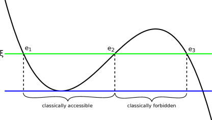
The perturbative energy levels of the QM system are solved from the quantum period of the cycle on ${\cal C}_{\text{QM}}$ associated to the classically accessible region of the potential $V(x)$, while the nonperturbative corrections are encoded in the Voros multiplier voross ; Voros1981 ; Silverstone1985:WKB , the quantum period of the cycle on ${\cal C}$ associated to the classically forbidden region. It was conjectured and verified in csm (see also cms ; cesv1 ) through examples of cubic potential and double well potential that the Voros multiplier together with the perturbative energy levels define the quantum free energy as an analogue of NS free energy and it can be solved from the NS holomorphic anomaly equations. This gives a relatively easy and systematic way to compute the Voros multiplier of a QM model. From this perspective, if we can find a 4d ${\cal N}=2$ theory whose SW curve coincides with the spectral curve ${\cal C}_{\text{QM}}$ of the QM model, and whose SW differential is

$$\Omega_{\text{SW}}=y(x){\rm d}x\ ,$$ (5.126)

which coincides with the exponential of the WKB solution to the QM model in the leading order, then naturally the periods of the QM model can be identified with those of the 4d theory, and the quantum free energy with the NS free energy. As advertised before, we will illustrate this idea for the QM models with the cubic potential and the double well potential. This identification of QM models with ${\cal N}=2$ theories gives a gauge theory justification for the algorithm proposed in csm . Note also that a connection between QM models with monic potentials and AD theories was noted in ito-shu in the context of ODE/IM correspondence Dorey:2007zx ; Dorey:1998pt .

5.1 The NS limit of $H_{0}$ theory and the cubic oscillator

Figure 2: The classically accessible and forbidden regions of a cubic potential.

The cubic oscillator is a one-dimensional quantum mechanical system characterised by the following potential

$$V(x)={x^{2}\over 2}-gx^{3}\ .$$ (5.127)

The spectral curve ${\cal C}_{\text{QM}}$ used to compute quantum periods and quantum free energy is csm

$${\cal C}_{\text{QM}}:\quad y^{2}=2\xi-x^{2}+2gx^{3}\ ,$$ (5.128)

where $\xi$ is identified with the energy of the QM model. We perform the following linear change of variables

$$x\to(2g)^{-1/3}x+1/(6g)\ .$$ (5.129)

then ${\cal C}_{\text{QM}}$ becomes

$$y^{2}=x^{3}-3cx+u\ ,$$ (5.130)

where

$$u=2\xi-\frac{1}{54g^{2}}\ ,\quad c={\frac{1}{3^{2}(2g)^{4/3}}}\ ,$$ (5.131)

which is precisely the SW curve for the $H_{0}$ theory (see eq (4.6) of ad1 , or (4.10) of betal ). $u$ is the Coulomb modulus, while $c$ is the scale parameter that controls the deformation away from the conformal point. In addition the SW differential of the $H_{0}$ theory is indeed of the form (5.126).

The QM model is studied in the semi-classical limit $\hbar\rightarrow 0$, in which case the period of the SW differential integrated around the classically accessible region (see Fig. 2) should shrink to zero csm . In the AD theory, this corresponds to a conifold point of the moduli space. The discriminant of the SW curve (5.130) is

$$\Delta=27(u^{2}-4c^{3})\ ,$$ (5.132)

and thus two conifold points exist

$$u_{\pm}=\pm 2c^{3/2}\ .$$ (5.133)

They correspond to the vanishing of the cycles around either the classically accessible region or the forbidden region. Since these two regions are exchanged to each other by $x\rightarrow-x$, the two conifold points are on equal footing, and we can choose either one. In the magnetic frame around the conifold point, say, $u_{+}$, the period $a_{D}$ is the good local coordinate and it has in general the form (up to a normalization constant)

$$\frac{{\rm d}a_{D}}{{\rm d}u}{~{}\propto~{}}\frac{1}{2\pi}\int_{e_{1}}^{e_{2}}\frac{{\rm d}x}{y}\ ,$$ (5.134)

where we have assumed $e_{1},e_{2},e_{3}$ to be the three branch points of (5.130) from left to right, as shown in Fig. 2. The integral above can be written as a hypergeometric function

$$\frac{{\rm d}a_{D}}{{\rm d}u}{~{}\propto~{}}\frac{1}{2}(e_{3}-e_{1})^{-1/2}{}_{2}F_{1}\left(\frac{1}{2},\frac{1}{2};1;z\right)\ ,$$ (5.135)

with

$$z=\frac{e_{2}-e_{1}}{e_{3}-e_{1}}\ .$$ (5.136)

Then following the same technique in Masuda:1996xj , we can transform the hypergeometric function to a form symmetric in $e_{1,2,3}$. The result is

$$\frac{{\rm d}a_{\rm D}}{{\rm d}u}{~{}\propto~{}}\frac{1}{2}(-{\cal D})^{-1/4}{}_{2}F_{1}\left(\frac{1}{12},\frac{5}{12};1;-\frac{27\Delta}{4{\cal D}^{3}}\right)\ ,$$ (5.137)

where $\Delta$ is the discriminant, while

$${\cal D}=-{1\over 2}\sum_{i<j}(e_{i}-e_{j})^{2}\ ,$$ (5.138)

which is $-9c$ in the case of (5.130). Therefore, we find

$${{\rm d}a_{\rm D}\over{\rm d}u}=\frac{\,{}_{2}F_{1}\left(\frac{1}{12},\frac{5}{12};1;-\frac{u^{2}}{4c^{3}}+1\right)}{{2^{1/3}}\cdot 3^{1/2}c^{1/4}}\ .$$ (5.139)

Likewise the prepotential $F_{0}^{\rm D}(a_{D})$ is computed in Masuda:1996xj ; betal and it reads (up to a normalization constant)

$$F_{0}^{\rm D}= {a_{D}^{2}\over 4}\left(\log{a_{D}\over 48\ 2^{2/3}3^{3/2}c^{5/4}}-{3}\right)+\frac{4}{5}2^{2/3}3^{3/2}c^{5/4}a_{D}+\frac{47a_{D}^{3}}{48\ 2^{2/3}3^{3/2}c^{5/4}}$$ (5.140)

$$+\frac{7717a_{D}^{4}}{248832\cdot 2^{1/3}c^{5/2}}+\mathcal{O}(a_{D}^{5})\ .$$

By using the dictionary (5.131) with $g=1$ we find (after normalization)

$$a_{\rm D}=\xi+\frac{15\xi^{2}}{4}+\frac{1155\xi^{3}}{16}+\frac{255255\xi^{4}}{128}+\cdots\ ,$$ (5.141)

and

$$F_{0}^{\rm D}={a_{D}^{2}\over 2}\left(\log{a_{D}\over 8}-{3\over 2}\right)+\frac{2a_{D}}{15}+\frac{47a_{D}^{3}}{8}+\frac{7717a_{D}^{4}}{128}+\mathcal{O}(a_{D}^{5})\ .$$ (5.142)

They are precisely the period associated to the classically accessible region and the planar component of the quantum free energy of the cubic oscillator given in csm (eq. (3.22) and eq. (3.23) respectively). Next the genus one quantum free energy is computed by csm

$${\cal F}^{\rm D}_{1}(a_{D})=-\frac{1}{24}\log\Delta\ ,$$ (5.143)

which is exactly how one would compute the genus one NS free energy for the gauge theory. In fact, both the quantum free energies of the cubic oscillator and the NS free energies of the $H_{0}$ theory are computed by the NS holomorphic anomaly equations, and they share the same initial conditions. Therefore the all order WKB solutions to the cubic oscillator are captured by the $H_{0}$ theory coupled to the $\Omega$ background in the NS limit.

Finally, we comment on the symmetry between the classically accessible region and forbidden region, which leads to that the quantum free energies are invariant under an $S$-transformation (see csm for more details). When translated to the gauge theory, it means the two conifold points $u_{\pm}$ are completely dual to each other, and the NS free energies expanded around these two singular points are identical.

5.2 The NS limit of $H_{1}$ theory and the double well potential

Figure 3: The classically accessible and forbidden regions of a double-well potential.

Let us consider the QM model with the double well potential

$$V(x)={x^{2}\over 2}(1+gx)^{2}\ .$$ (5.144)

The associated spectral curve is, after scaling and shifting to put it in a symmetric form csm

$${\cal C}_{\text{QM}}:\quad y^{2}=(x^{2}-a_{+}^{2})(a_{-}^{2}-x^{2})\ ,$$ (5.145)

where

$$a_{\pm}^{2}=\frac{1}{4}\left(\pm\sqrt{32\xi}+g^{-1}\right)\ .$$ (5.146)

Through the scaling

$$x\to\frac{{\rm e}^{\frac{{\rm i}\pi}{4}}x}{\sqrt{g}}\ ,$$ (5.147)

we can write (5.145) as

$$y^{2}=x^{4}+4cx^{2}+2mx+u\ ,$$ (5.148)

where

$$u=\frac{1}{16}\left(32\xi-g^{-2}\right)\ ,\quad c=\frac{{\rm i}}{8}\,g^{-1},\quad m=0\ ,$$ (5.149)

and this is precisely the SW curve (2.48) for the $H_{1}$ theory, and as we have seen in Sec. 2.2 the SW differential $\Omega_{H_{1}}$ of this theory is of the form (5.126).

In the QM model, the classically accessible regions are indicated in Fig. 3. In the semi-classical limit, the period of $\Omega_{H_{1}}$ around this region vanishes, corresponding to a conifold point of the moduli space of the SW curve. We have seen in Sec. 2.2 that there are three conifold points $u=u^{(i)},i=1,2,3$. Among them, $u^{(2,3)}$ are due to the vanishing of either of the two branch cuts, and they correspond to the two classically accessible regions of the double-well potential, while $u^{(1)}$ which is due to the merger of the two branch cuts, corresponds to the classically forbidden region. Therefore, the semi-classical limit corresponds to either $u^{(2)}$ or $u^{(3)}$.

In the magnetic frame in the vicinity of the singular point $u^{(2)}$, the period $a_{D}$ is the locally good coordinate, and it can be computed by using the generic formula in Masuda:1996xj (up to a normalization constant)

$$\frac{{\rm d}a_{D}}{{\rm d}u}=\frac{1}{2}(-{\cal D})^{-1/4}{}_{2}F_{1}\left(\frac{1}{12},\frac{5}{12};1;-\frac{27\Delta}{4{\cal D}^{3}}\right)\ ,$$ (5.150)

where $\Delta$ is the discriminant, and ${\cal D}$ is given by

$${\cal D}=-\frac{1}{2}\left((e_{1}-e_{2})^{2}(e_{3}-e_{4})^{2}+(e_{1}-e_{3})^{2}(e_{2}-e_{4})^{2}+(e_{1}-e_{4})^{2}(e_{2}-e_{3})^{2}\right)\ ,$$ (5.151)

with $e_{i},i=1,2,3,4$ being the four branch points (see Fig. 3). In the case of (5.148), we have

$$\frac{{\rm d}a_{D}}{{\rm d}u}=\frac{\,{}_{2}F_{1}\left(\frac{1}{12},\frac{5}{12};1;\frac{27u\left(4c^{2}-u\right)^{2}}{\left(4c^{2}+3u\right)^{3}}\right)}{2\sqrt{2}(3u+4c^{2})^{1/4}}\ .$$ (5.152)

After applying the dictionary (5.149) (g is set to 1) and expanding w.r.t. $\xi$, we get (after normalization)

$$a_{D}=\xi+3\xi^{2}+35\xi^{3}+\frac{1155\xi^{4}}{2}+\frac{45045\xi^{5}}{4}+\frac{969969\xi^{6}}{4}+{\cal O}(\xi^{7})\ .$$ (5.153)

The prepotential $F_{0}^{\rm D}(a_{D})$ can be found in Masuda:1996xj ; betal , and when $m=0$ it reads

$$F_{0}^{D}=a_{D}^{2}\log\left(\frac{a_{D}}{2}\right)+\frac{a_{D}}{3}-\frac{3a_{D}^{2}}{2}+\frac{17a_{D}^{3}}{3}+\frac{125a_{D}^{4}}{4}+\mathcal{O}(a_{D}^{5})\ .$$ (5.154)

They indeed agree with the period and genus zero quantum free energy given in csm . Furthermore, the genus one quantum free energy is computed by (5.143) csm , and this is how one would compute the genus one NS free energy for the gauge theory. Higher genus free energies would also agree, since they are computed both in the QM model with double well potential and in the $H_{1}$ theory from the NS holomorphic anomaly equations and they share the same initial data. As a result, the all order WKB solutions to the double well QM model are captured by the $H_{1}$ theory coupled to the $\Omega$ background in the NS limit.

6 Summary and open questions

It is an interesting problem to look for matrix model representations of supersymmetric gauge theories. It has been proposed in tc12 ; Rim:2012tf that many Argyres-Douglas (AD) theories can be represented by hermitian matrix models with rational/logarithmic potentials. In this paper we show in detail that the well-studied $\beta$-deformed cubic matrix model in the generic two-cut phase computes the partition function of the $H_{1}$ AD theory coupled to the $\Omega$ background in the magnetic frame. Then we further extend this relation to integrable non-linear ODEs. According to the Painlevé/gauge correspondence betal , the $H_{1}$ AD theory in the self-dual $\Omega$ background is expected to compute the $\tau$ function of the Painlevé II equation. By combining these two observations we showed that, in the non-deformed $\beta=1$ case, the two-cut cubic matrix model computes the $\tau$ function of the Painlevé II equation. Using this connection with matrix model, we studied in detail the $\tau$ function solution to Painlevé II proposed in betal ; Its:2016jkt , and we found that the summand (3.85) appearing in this solution is in fact an asymptotic series with zero radius of convergence. Relatedly, when considering the $\tau$ function one has to sum over all integer shifts as illustrated in equation (3.84). We found that, from the resurgence perspective, this summation corresponds to a sum over trans-series which, in the matrix model language, amounts to a sum over all possible eigenvalues tunnellings or a sum over all filling fractions similar to bde ; em ; eynard . Furthermore our analysis also shows explicitly how the $n^{\rm th}$ instanton sector of the PII solution in (4.107) is completely determined by the same function as the perturbative sector, namely the term $n=0$ in (4.104) which is computed by the two-cut cubic model via (3.94) and (3.92).

We note that the connection between Painlevé equations and hermitian matrix models has been explored before in the literature in particular in connection with 2d gravity Douglas:1989ve ; Brezin:1990rb ; Gross:1989vs ; Kharchev:1991cy . See DiFrancesco:1993cyw for a more exhaustive list of references. For instance in dss ; cmo it was found that the quartic matrix model in the double scaling limit is related to the Painlevé II equation (4.101) at $\theta=1/2$. Likewise the Gross–Witten–Wadia model also makes contact with Painlevé II in a particular double scaling limit. See for instance mmnp and reference therein. Other models with external fields were also introduced in this context; see for instance Mironov:1994mv and reference therein. From that viewpoint what distinguishes our matrix model representation for Painlevé II from the previous ones is that, after summing over all possible eigenvalues tunneling, it computes the $\tau$ function of the Painlevé II without taking the double scaling limit nor adding any external fields and that it is valid for generic values of $\theta$ and integration constants $(\nu,\rho)$.

Finally we explored the Nekrasov-Shatashvili phase of the $H_{0}$ and $H_{1}$ AD theories and we showed that they determine the spectral properties of corresponding quantum mechanical systems with cubic and double well potentials respectively. This provides a gauge theory justification for the all order WKB solutions from holomorphic anomaly equations proposed in csm for these two quantum mechanical models.

There are still many open questions that remain to be addressed. One of the obvious questions is whether one can find a similar matrix model representation for the solutions to PI and PIV presented in betal ; Lisovyy:2016qig . Besides, the matrix model for the $H_{1}$ theory is studied in the weak coupling limit, very far away from the conformal point. It would be interesting to explore the strong coupling limit $g_{s}/m\to 0$, probably following Cordova:2016jlu , and see if one can construct in this way solutions to Painlevé II for small times. Furthermore it would be interesting to study in more detail the Borel resummation of the perturbative sector of the $\tau$-function, whose coefficients can be computed from the two-cut cubic matrix model, similar to what we have done at the end of section 4.

Finally, concerning the relation between the AD theories and the WKB solutions in terms of holomorphic equations csm . Although in the case of cubic and double well potentials we provide the existence of dual AD theories as a justification for the latter, the connection between WKB solutions and holomorphic anomaly equations is expected to be more basic and holds beyond the existence of a dual supersymmetric gauge theory as explained in csm . In that perspective it would be interesting to further investigate the algorithm presented in csm ; cms for more generic quantum mechanical systems with no gauge theory connection.

Appendix A The $D_{k}$ coefficients

We list here some of the $D_{k}$ coefficients as computed from the matrix model

$$D_{4}(\nu,\theta) =\frac{\left(1008845824-45278208\theta^{2}\right)\nu^{10}}{161243136}+\frac{\left(8989056\theta^{4}-440169984\theta^{2}+4500384000\right)\nu^{8}}{161243136}$$ (A.155)

$$+\frac{\left(-793152\theta^{6}+65329920\theta^{4}-1536680448\theta^{2}+8573056768\right)\nu^{6}}{161243136}$$

$$+\frac{\left(26244\theta^{8}-3517344\theta^{6}+149049216\theta^{4}-2119879296\theta^{2}+4076024896\right)\nu^{4}}{161243136}$$

$$+\frac{\left(32076\theta^{8}-3181680\theta^{6}+97473744\theta^{4}-731835072\theta^{2}+287635968\right)\nu^{2}}{161243136}$$

$$+\frac{3267\theta^{8}-338472\theta^{6}+7102512\theta^{4}-29735424\theta^{2}}{161243136}+\frac{83521\nu^{12}}{157464}\ .$$

$$D_{5}(\nu,\theta)= -\frac{{\rm i}\left(114050775040-3848647680\theta^{2}\right)\nu^{13}}{29023764480}$$ (A.156)

$$-\frac{{\rm i}\left(1018759680\theta^{4}-64867691520\theta^{2}+923488394240\right)\nu^{11}}{29023764480}$$

$$-\frac{{\rm i}\left(-134835840\theta^{6}+13976643840\theta^{4}-437858730240\theta^{2}+3866409244160\right)\nu^{9}}{29023764480}$$

$$-\frac{{\rm i}\left(8922960\theta^{8}-1375937280\theta^{6}+72318366720\theta^{4}-1463686214400\theta^{2}+8148525547264\right)\nu^{7}}{29023764480}$$

$$-\frac{{\rm i}\left(-236196\theta^{10}+56307960\theta^{8}-4676382720\theta^{6}\right)\nu^{5}}{29023764480}$$

$$-\frac{{\rm i}\left(167309213760\theta^{4}-2324529313344\theta^{2}+5918924547200\right)\nu^{5}}{29023764480}$$

$$-\frac{{\rm i}\left(-481140\theta^{10}+85004100\theta^{8}-5528478960\theta^{6}\right)\nu^{3}}{29023764480}$$

$$-\frac{{\rm i}\left(150410948640\theta^{4}-1265133321600\theta^{2}+1004626036224\right)\nu^{3}}{29023764480}$$

$$-\frac{{\rm i}\left(-147015\theta^{10}+26062830\theta^{8}-1548868608\theta^{6}\right)\nu}{29023764480}$$

$$-\frac{{\rm i}\left(30819065760\theta^{4}-151899224832\theta^{2}+12454041600\right)\nu}{29023764480}-\frac{1419857{\rm i}\nu^{15}}{7085880}\ .$$

$$D_{6}(\nu,\theta) =\frac{\left(628099301376\theta^{2}-23231463702528\right)\nu^{16}}{12538266255360}$$ (A.157)

$$+\frac{\left(-207826974720\theta^{4}+16289288110080\theta^{2}-295207026769920\right)\nu^{14}}{12538266255360}$$

$$+\frac{\left(36675348480\theta^{6}-4596550456320\theta^{4}+179123561349120\theta^{2}-2098472385310720\right)\nu^{12}}{12538266255360}$$

$$+\frac{\left(-3640567680\theta^{8}+657251573760\theta^{6}-41664329740800\theta^{4}\right)\nu^{10}}{12538266255360}$$

$$+\frac{\left(1072630221373440\theta^{2}-8861527274778624\right)\nu^{10}}{12538266255360}$$

$$+\frac{\left(192735936\theta^{10}-48583592640\theta^{8}+4552446758400\theta^{6}\right)\nu^{8}}{12538266255360}$$

$$+\frac{\left(-195592116614400\theta^{4}+3680491078803456\theta^{2}-20941693135389696\right)\nu^{8}}{12538266255360}$$

$$+\frac{\left(-4251528\theta^{12}+1617050304\theta^{10}-224210592000\theta^{8}+14857834717440\theta^{6}\right)\nu^{6}}{12538266255360}$$

$$+\frac{\left(-486010693602432\theta^{4}+6759704932125696\theta^{2}-21152656059375104\right)\nu^{6}}{12538266255360}$$

$$+\frac{\left(-12990780\theta^{12}+3609891360\theta^{10}-399130422480\theta^{8}+21707906542848\theta^{6}\right)\nu^{4}}{12538266255360}$$

$$+\frac{\left(-563405245951680\theta^{4}+5235646863930624\theta^{2}-6692702742982656\right)\nu^{4}}{12538266255360}$$

$$+\frac{\left(-7938810\theta^{12}+2144018160\theta^{10}-224279061624\theta^{8}+10830074974272\theta^{6}\right)\nu^{2}}{12538266255360}$$

$$+\frac{\left(-215197143901056\theta^{4}+1245163592706048\theta^{2}-361928925941760\right)\nu^{2}}{12538266255360}$$

$$+\frac{-539055\theta^{12}+157546620\theta^{10}-17570163600\theta^{8}+746102664000\theta^{6}}{12538266255360}$$

$$+\frac{-11086283013120\theta^{4}+40217382420480\theta^{2}}{12538266255360}-\frac{24137569\nu^{18}}{382637520}$$

$$D_{7}(\nu,\theta) =\frac{{\rm i}\left(2209420712869888-49829211242496\theta^{2}\right)\nu^{19}}{3159643096350720}+\frac{410338673{\rm i}\nu^{21}}{24106163760}$$ (A.158)

$$+\frac{{\rm i}\left(19785127993344\theta^{4}-1841697992687616\theta^{2}+40411929818136576\right)\nu^{17}}{3159643096350720}$$

$$+\frac{{\rm i}\left(-4364366469120\theta^{6}+642254718099456\theta^{4}-29878724974952448\theta^{2}+431294717560340480\right)\nu^{15}}{3159643096350720}$$

$$+\frac{{\rm i}\left(-277714792149258240\theta^{2}+2935883132605079552\right)\nu^{13}}{3159643096350720}$$

$$+\frac{{\rm i}\left(577636738560\theta^{8}-120384194595840\theta^{6}+8952988529479680\theta^{4}\right)\nu^{13}}{3159643096350720}$$

$$+\frac{{\rm i}\left(+69401564740730880\theta^{4}-1607864190545055744\theta^{2}+12896647995981582336\right)\nu^{11}}{3159643096350720}$$

$$+\frac{{\rm i}\left(-45871152768\theta^{10}+12896334259200\theta^{8}-1378404422115840\theta^{6}\right)\nu^{11}}{3159643096350720}$$

$$+\frac{{\rm i}\left(+321246107010984960\theta^{4}-5827275251745389568\theta^{2}+34254091748212793344\right)\nu^{9}}{3159643096350720}$$

$$+\frac{{\rm i}\left(2023727328\theta^{12}-765556795584\theta^{10}+113105000211840\theta^{8}-8358622716568320\theta^{6}\right)\nu^{9}}{3159643096350720}$$

$${+}\frac{{\rm i}\left(1707034285647117\theta^{4}-24071708860929693\theta^{2}+88226082084596078\right)\nu^{7}}{6171177922560}$$

$$-\frac{{\rm i}\left(59049\theta^{8}-33332796\theta^{6}+7014457296\theta^{4}-744878628760\theta^{2}+43365988680784\right)\theta^{6}\nu^{7}}{4875992432640}$$

$$+\frac{{\rm i}\left(155714834383535\theta^{4}-1576621725969740\theta^{2}+2849012960896848\right)\nu^{5}}{391820820480}$$

$$-\frac{{\rm i}\left(72171\theta^{8}-29238408\theta^{6}+4915342260\theta^{4}-438283228448\theta^{2}+21688585670448\right)\theta^{6}\nu^{5}}{1393140695040}$$

$$+\frac{{\rm i}\left(107917467861539\theta^{4}-723209858672616\theta^{2}+440213751859680\right)\nu^{3}}{457124290560}$$

$$-\frac{{\rm i}\left(441045\theta^{8}-169143420\theta^{6}+26848410372\theta^{4}-2222362258648\theta^{2}+97346044324736\right)\theta^{6}\nu^{3}}{8358844170240}$$

$$+\frac{{\rm i}\left(300249586861\theta^{4}-1289393108560\theta^{2}+81477396000\right)\nu}{8465264640}$$

$$-\frac{{\rm i}\left(419265\theta^{8}-168824810\theta^{6}+28035354984\theta^{4}-2301504916992\theta^{2}+88873063642496\right)\theta^{6}\nu}{39007939461120}$$

Likewise it is very easy to obtain higher $D_{k}$, nevertheless the expressions are quite cumbersome and we decided not to write them down explicitly.

References

- (1) P. C. Argyres and M. R. Douglas, New phenomena in SU(3) supersymmetric gauge theory, Nucl. Phys. B448 (1995) 93–126, [hep-th/9505062].
- (2) P. C. Argyres, M. R. Plesser, N. Seiberg and E. Witten, New N=2 superconformal field theories in four-dimensions, Nucl. Phys. B461 (1996) 71–84, [hep-th/9511154].
- (3) T. Nishinaka and C. Rim, Matrix models for irregular conformal blocks and Argyres-Douglas theories, JHEP 10 (2012) 138, [1207.4480].
- (4) C. Rim, Irregular conformal block and its matrix model, 1210.7925.
- (5) K. Kajiwara, T. Masuda, M. Noumi, Y. Ohta and Y. Yamada, Cubic pencils and Painleve Hamiltonians, nlin/0403009.
- (6) O. Gamayun, N. Iorgov and O. Lisovyy, Conformal field theory of Painlevé VI, JHEP 10 (2012) 038, [1207.0787].
- (7) O. Gamayun, N. Iorgov and O. Lisovyy, How instanton combinatorics solves Painlevé VI, V and IIIs, J. Phys. A46 (2013) 335203, [1302.1832].
- (8) G. Bonelli, O. Lisovyy, K. Maruyoshi, A. Sciarappa and A. Tanzini, On Painlevé/gauge theory correspondence, 1612.06235.
- (9) V. A. Kazakov, I. K. Kostov and N. A. Nekrasov, D particles, matrix integrals and KP hierarchy, Nucl.Phys. B557 (1999) 413–442, [hep-th/9810035].
- (10) P. Di Francesco, P. H. Ginsparg and J. Zinn-Justin, 2-D Gravity and random matrices, Phys. Rept. 254 (1995) 1–133, [hep-th/9306153].
- (11) F. Cachazo, K. A. Intriligator and C. Vafa, A Large N duality via a geometric transition, Nucl. Phys. B603 (2001) 3–41, [hep-th/0103067].
- (12) A. Klemm, M. Marino and S. Theisen, Gravitational corrections in supersymmetric gauge theory and matrix models, JHEP 03 (2003) 051, [hep-th/0211216].
- (13) A. Klemm, M. Mariño and M. Rauch, Direct Integration and Non-Perturbative Effects in Matrix Models, JHEP 10 (2010) 004, [1002.3846].
- (14) M.-x. Huang, Dijkgraaf-Vafa conjecture and -deformed matrix models, JHEP 07 (2013) 173, [1305.1103].
- (15) R. Schiappa and R. Vaz, The Resurgence of Instantons: Multi-Cut Stokes Phases and the Painleve II Equation, Commun. Math. Phys. 330 (2014) 655–721, [1302.5138].
- (16) M. Marino, Nonperturbative effects and nonperturbative definitions in matrix models and topological strings, JHEP 0812 (2008) 114, [0805.3033].
- (17) A. Its, O. Lisovyy and A. Prokhorov, Monodromy dependence and connection formulae for isomonodromic tau functions, 1604.03082.
- (18) S. Codesido and M. Marino, Holomorphic Anomaly and Quantum Mechanics, J. Phys. A51 (2018) 055402, [1612.07687].
- (19) R. Dijkgraaf, S. Gukov, V. A. Kazakov and C. Vafa, Perturbative analysis of gauged matrix models, Phys. Rev. D68 (2003) 045007, [hep-th/0210238].
- (20) K. Maruyoshi, -deformed matrix models and the 2d/4d correspondence, in New Dualities of Supersymmetric Gauge Theories (J. Teschner, ed.), pp. 121–157. 2016. 1412.7124. DOI.
- (21) G. Bonelli, K. Maruyoshi and A. Tanzini, Quantum Hitchin Systems via beta-deformed Matrix Models, 1104.4016.
- (22) T. Masuda and H. Suzuki, Periods and prepotential of N=2 SU(2) supersymmetric Yang-Mills theory with massive hypermultiplets, Int. J. Mod. Phys. A12 (1997) 3413–3431, [hep-th/9609066].
- (23) G. Bonelli, K. Maruyoshi and A. Tanzini, Wild Quiver Gauge Theories, JHEP 02 (2012) 031, [1112.1691].
- (24) D. Gaiotto and J. Teschner, Irregular singularities in Liouville theory and Argyres-Douglas type gauge theories, I, JHEP 12 (2012) 050, [1203.1052].
- (25) G. Akemann, Higher genus correlators for the Hermitian matrix model with multiple cuts, Nucl. Phys. B482 (1996) 403–430, [hep-th/9606004].
- (26) M. Bershadsky, S. Cecotti, H. Ooguri and C. Vafa, Holomorphic anomalies in topological field theories, Nucl.Phys. B405 (1993) 279–304, [hep-th/9302103].
- (27) B. Eynard and N. Orantin, Invariants of algebraic curves and topological expansion, Commun.Num.Theor.Phys. 1 (2007) 347–452, [math-ph/0702045].
- (28) M.-x. Huang and A. Klemm, Direct integration for general backgrounds, Adv.Theor.Math.Phys. 16 (2012) 805–849, [1009.1126].
- (29) D. Krefl and J. Walcher, Extended Holomorphic Anomaly in Gauge Theory, Lett. Math. Phys. 95 (2011) 67–88, [1007.0263].
- (30) N. A. Nekrasov, Seiberg-Witten prepotential from instanton counting, Adv.Theor.Math.Phys. 7 (2004) 831–864, [hep-th/0206161].
- (31) N. Nekrasov and A. Okounkov, Seiberg-Witten theory and random partitions, Prog. Math. 244 (2006) 525–596, [hep-th/0306238].
- (32) M.-x. Huang and A. Klemm, Holomorphic Anomaly in Gauge Theories and Matrix Models, JHEP 09 (2007) 054, [hep-th/0605195].
- (33) M.-x. Huang and A. Klemm, Holomorphicity and Modularity in Seiberg-Witten Theories with Matter, JHEP 07 (2010) 083, [0902.1325].
- (34) G. Bonelli, A. Grassi and A. Tanzini, Seiberg–Witten theory as a Fermi gas, Lett. Math. Phys. 107 (2017) 1–30, [1603.01174].
- (35) G. Bonelli, A. Grassi and A. Tanzini, New results in theories from non-perturbative string, 1704.01517.
- (36) M. Marino and S. Zakany, Matrix models from operators and topological strings, Annales Henri Poincare 17 (2016) 1075–1108, [1502.02958].
- (37) R. Kashaev, M. Marino and S. Zakany, Matrix models from operators and topological strings, 2, Annales Henri Poincare 17 (2016) 2741–2781, [1505.02243].
- (38) S. Codesido, J. Gu and M. Marino, Operators and higher genus mirror curves, JHEP 02 (2017) 092, [1609.00708].
- (39) S. Codesido, A. Grassi and M. Marino, Spectral Theory and Mirror Curves of Higher Genus, Annales Henri Poincare 18 (2017) 559–622, [1507.02096].
- (40) G. Bonelli, A. Grassi and A. Tanzini, Quantum curves and -deformed Painlevé equations, 1710.11603.
- (41) A. Mironov and A. Morozov, On determinant representation and integrability of Nekrasov functions, Phys. Lett. B773 (2017) 34–46, [1707.02443].
- (42) A. Mironov and A. Morozov, q-Painleve equation from Virasoro constraints, 1708.07479.
- (43) A. Its, O. Lisovyy and Yu. Tykhyy, Connection problem for the sine-Gordon/Painlevé III tau function and irregular conformal blocks, Int. Math. Res. Notices 18 (2015) 8903–8924, [1403.1235].
- (44) M. Marino, R. Schiappa and M. Weiss, Multi-Instantons and Multi-Cuts, J.Math.Phys. 50 (2009) 052301, [0809.2619].
- (45) G. Bonnet, F. David and B. Eynard, Breakdown of universality in multicut matrix models, J.Phys. A33 (2000) 6739–6768, [cond-mat/0003324].
- (46) B. Eynard and M. Marino, A Holomorphic and background independent partition function for matrix models and topological strings, J.Geom.Phys. 61 (2011) 1181–1202, [0810.4273].
- (47) B. Eynard, Large N expansion of convergent matrix integrals, holomorphic anomalies, and background independence, JHEP 0903 (2009) 003, [0802.1788].
- (48) G. Felder and R. Riser, Holomorphic matrix integrals, Nucl. Phys. B691 (2004) 251–258, [hep-th/0401191].
- (49) N. A. Nekrasov and S. L. Shatashvili, Quantization of Integrable Systems and Four Dimensional Gauge Theories, 0908.4052.
- (50) A. Grassi and J. Gu, BPS relations from spectral problems and blowup equations, 1609.05914.
- (51) A. Mironov and A. Morozov, Nekrasov Functions from Exact BS Periods: The Case of SU(N), J.Phys. A43 (2010) 195401, [0911.2396].
- (52) G. Basar, G. V. Dunne and M. Unsal, Quantum Geometry of Resurgent Perturbative/Nonperturbative Relations, JHEP 05 (2017) 087, [1701.06572].
- (53) A. Mironov and A. Morozov, Nekrasov Functions and Exact Bohr-Zommerfeld Integrals, JHEP 1004 (2010) 040, [0910.5670].
- (54) M. Aganagic, M. C. Cheng, R. Dijkgraaf, D. Krefl and C. Vafa, Quantum Geometry of Refined Topological Strings, JHEP 1211 (2012) 019, [1105.0630].
- (55) N. Nekrasov, Five dimensional gauge theories and relativistic integrable systems, Nucl. Phys. B531 (1998) 323–344, [hep-th/9609219].
- (56) A. Grassi, Y. Hatsuda and M. Marino, Topological Strings from Quantum Mechanics, Annales Henri Poincare 17 (2016) 3177–3235, [1410.3382].
- (57) J. Gu, A. Klemm, M. Marino and J. Reuter, Exact solutions to quantum spectral curves by topological string theory, JHEP 10 (2015) 025, [1506.09176].
- (58) X. Wang, G. Zhang and M.-x. Huang, New Exact Quantization Condition for Toric Calabi-Yau Geometries, Phys. Rev. Lett. 115 (2015) 121601, [1505.05360].
- (59) K. Sun, X. Wang and M.-x. Huang, Exact Quantization Conditions, Toric Calabi-Yau and Nonperturbative Topological String, JHEP 01 (2017) 061, [1606.07330].
- (60) A. Grassi and M. Marino, The complex side of the TS/ST correspondence, 1708.08642.
- (61) J. Dunham, The Wentzel-Brillouin-Kramers method of solving the wave equation, Phys. Rev. 41 (1932) 713–720.
- (62) C. M. Bender, K. Olaussen and P. Wang, Numerological analysis of the WKB approximation in large order, Phys. Rev. D 16 (1977) 1740–1748.
- (63) A. Galindo and P. Pascual, Quantum Mechanics, vol. 2. Springer-Verlag, 1990.
- (64) A. Voros, The return of the quartic oscillator. The complex WKB method, Ann. Inst. H. Poincaré A 39 (1983) 211.
- (65) A. Voros, Spectre de l’équation de Schrödinger et méthode BKW. Publications Mathématiques d’Orsay, 1981.
- (66) H. J. Silverstone, JWKB connection-formula problem revisited via Borel summation, Phys. Rev. Lett. 55 (1985) 2523.
- (67) S. Codesido, M. Marino and R. Schiappa, Non-Perturbative Quantum Mechanics from Non-Perturbative Strings, 1712.02603.
- (68) R. Couso-Santamaría, J. D. Edelstein, R. Schiappa and M. Vonk, Resurgent Transseries and the Holomorphic Anomaly, Annales Henri Poincare 17 (2016) 331–399, [1308.1695].
- (69) A. Grassi, Spectral determinants and quantum theta functions, J. Phys. A49 (2016) 505401, [1604.06786].
- (70) K. Ito and H. Shu, ODE/IM correspondence and the Argyres-Douglas theory, JHEP 08 (2017) 071, [1707.03596].
- (71) P. Dorey, C. Dunning and R. Tateo, The ODE/IM Correspondence, J. Phys. A40 (2007) R205, [hep-th/0703066].
- (72) P. Dorey and R. Tateo, Anharmonic oscillators, the thermodynamic Bethe ansatz, and nonlinear integral equations, J. Phys. A32 (1999) L419–L425, [hep-th/9812211].
- (73) M. R. Douglas and S. H. Shenker, Strings in Less Than One-Dimension, Nucl. Phys. B335 (1990) 635.
- (74) E. Brezin and V. A. Kazakov, Exactly Solvable Field Theories of Closed Strings, Phys. Lett. B236 (1990) 144–150.
- (75) D. J. Gross and A. A. Migdal, Nonperturbative Two-Dimensional Quantum Gravity, Phys. Rev. Lett. 64 (1990) 127.
- (76) S. Kharchev, A. Marshakov, A. Mironov, A. Morozov and A. Zabrodin, Towards unified theory of 2-d gravity, Nucl. Phys. B380 (1992) 181–240, [hep-th/9201013].
- (77) M. R. Douglas, N. Seiberg and S. H. Shenker, Flow and instability in quantum gravity, Phys. Lett. B 244 (1990) 381–386.
- (78) C.Crnković and G. Moore, Multicritical multi-cut matrix models, Phys. Lett. B 257 (1991) .
- (79) A. Mironov, A. Morozov and G. W. Semenoff, Unitary matrix integrals in the framework of generalized Kontsevich model. 1. Brezin-Gross-Witten model, Int. J. Mod. Phys. A11 (1996) 5031–5080, [hep-th/9404005].
- (80) O. Lisovyy and J. Roussillon, On the connection problem for Painlevé I, J. Phys. A50 (2017) 255202, [1612.08382].
- (81) C. Cordova, B. Heidenreich, A. Popolitov and S. Shakirov, Orbifolds and Exact Solutions of Strongly-Coupled Matrix Models, 1611.03142.