Path probabilities for consecutive measurements, and certain "quantum paradoxes"
Abstract
ABSTRACT:
We consider a finite-dimensional quantum system, making a transition between known initial and final states.
The outcomes of several accurate measurements, which could be made in the interim,
define virtual paths, each endowed with a probability amplitude.
If the measurements are actually made, the paths, which may now be called "real", acquire also the probabilities,
related to the frequencies, with which a path is seen to be travelled in a series of identical trials.
Different sets of measurements, made on the same system, can produce
different, or incompatible, statistical ensembles, whose conflicting attributes
may, although by no means should, appear "paradoxical".
We describe in detail the ensembles, resulting from intermediate measurements of mutually commuting, or non-commuting, operators,
in terms of the real paths produced. In the same manner, we analyse the Hardy’s and the "three box" paradoxes,
the photon’s past in an interferometer, the "quantum Cheshire cat" experiment, as well as the closely related subject of
"interaction-free measurements". It is shown that, in all these cases, inaccurate "weak measurements" produce no real paths,
and yield only limited information about the virtual paths’ probability amplitudes.
I Introduction
Recently, there has been significant interest in the properties of a pre-and post-selected quantum systems,
and, in particular, in the description of such systems during the time between the preparation, and
the arrival in the pre-determined final state (see, for example Chin and the Refs. therein). Intermediate state of the system can be probed by
performing, one after another, measurements of various physical quantities.
Although produced from the same quantum system, statistical ensembles, resulting from different sets of measurements, are known to have
conflicting and seemingly incompatible qualities. These conflicts have, in turn, led to the discussion of certain "quantum paradoxes",
allegedly specific to a system, subjected to post-selection.
Such is, for example, the "three box paradox" 3Ba -3Bd , claiming that a particle
can be, at the same time, at two different locations "with certainty". A similarly "paradoxical" suggestion that a photon could, on its way to detection,
have visited the places it had "never entered, nor left, was made in Nest1 -Nest2 , and further discussed in Nest3 -Nest6 . In the discussion of the Hardy’s paradox HARDY1 -HARDY4 the particle
is suspected of simultaneously "being and not being" at the same location HARDY2 . The so called "quantum Cheshire cat" scheme CAT1 -CAT3
promises "disembodiment of physical properties from the object they belong to".
One can easily dismiss a "paradox" of this type simply by noting that the conflicting features are never observed in the same experimental setup, and therefore, never occur "simultaneously" 3Bd , HARDY4 , Stapp1 , Unruh , Stapp2 , Kastner .
(We agree: one can use a piece of plasticine to make a ball, or a cube, but should not claim that an object can be a ball and a cube at the same time.) There have been attempts to ascertain "simultaneous presence" of the conflicting attributes by subjecting the system
to weakly perturbing, or "weak" measurements 3Ba , Nest1 , HARDY2 , CAT1 . However, such measurements only probe the values of
the relative probability amplitudes, corresponding to the processes of interest CAT4 , CAT5 , DSann and by no means prove that these processes
are, indeed, taking place at the same time. Furthermore, confusing these amplitudes with the value of a physical quantity,
may lead to such unhelpful concepts as "negative numbers of particles" HARDY2 , "negative durations" spent by a non-relativistic particle in a specified region of space TRAV . or "apparently superluminal"
transmission of a tunnelling particle across a potential barrier Ann .
Similar questions can be asked about macroscopic quantum systems, such as superconducting flux qubits LG1 .
The answers are often formulated in terms of the Leggett-Garg inequalities LG2 , which restrict the values of correlators of physical observables, under the assumption that macroscopic superpositions cannot persist for some fundamental
reason (for a review see LG3 , and for recent developments LG4 ).
It is not our intention to compile an exhaustive list of relevant literature, or to discuss all aspects of the subject in great detail.
The main purpose of this paper is
to describe consecutive quantum measurements in a simple language, relying only on the most basic principles and concepts of elementary quantum mechanics. The brief introduction, already made, may have helped to convince the reader that such a description would indeed be desirable.
We start from a simple premise. With the initial and final states of the system fixed, there are many measurements which could,
in principle, be performed in the interim. Connecting results of possible measurements,
performed at different times,
defines a virtual path, which a system could follow. For each virtual path
quantum mechanics provides a complex valued probability amplitude .
If the said measurements are actually made, the outcomes become a sequence of observable events,
the path acquires a probability, ,
and becomes real. (We use "real" as a natural complement to "virtual".)
The set of all real paths, possible final destinations, and the corresponding probabilities, together define a classical statistical ensemble.
We note that a similar ensemble could, in principle, be constructed also by purely classical means.
For example, it is not difficult to imagine a gun, whose bullets would arrive at a point on the screen
with exactly the same probability, as the electrons in the Young’s double slit experiment.
For someone, interested only in the number of particles per square centimetre,
the two ensembles would be identical.
The quantum side of the discussion is, therefore, limited to the details of the ensemble’s preparation.
In the previous example, the same distribution can be achieved by aiming the gun at different angles,
and varying the frequency of the shots, or by using quantum interference.
In the following, we will be interested in exploiting the quantum properties of a system, and will return
to a classical analogue only occasionally.
Two well known features of conventional quantum measurements Real3 ,
are easily translated into the language of quantum paths.
The fact that the results of a measurement cannot "pre-exist" the measurement Merm , means that different sets of measurements
are able to produce different, and in some sense incompatible, statistical ensembles.
The fact that quantum mechanics is non-local was summarised in Merm as follows:
"…the value assigned to an observable must depend on the complete experimental arrangement
under which it is measured, even when two arrangements differ only far from the region in which the value is ascertained.
Thus, we can expect that a single change, made in a distant part of the setup, may produce a new network of real paths, all parts of which will be incompatible
with the original ensemble.
Throughout the rest of the paper, we will attempt to make the proposed description of consecutive
quantum measurements sufficiently precise, explore its usefulness, and review, with its help, some of the quantum "paradoxes",
already mentioned above.
The rest of the paper is organised as follows.
In Sect. II we continue with the introduction, and revisit Feynman’s example Feyns , used to demonstrate that quantum probabilities cannot
pre-exist the measurement, and must be produced in its course.
In Sect. III we describe one way to decide whether two given sets of averages can belong to the same statistical ensemble.
In Sect. IV we show that the results in Sect. I fail the test of Sect. II, and would require the use of at least two different ensembles,
in order to be reproduced by purely classical means.
In Sect. V we show how a statistical ensemble,
describing a system which can reach its final destination in several different ways, is produced by applying a sequence of accurate von Neumann measurements.
In Sect. VI we consider an example, in which the real paths are produced by measurements of commuting operators, acting in a three-dimensional Hilbert space.
In Section VII we introduce non-perturbing (non-demolition) measurements, capable of providing a more detailed description of a real path, without altering the ensemble.
In Sect. VIII we briefly discuss the "three-box" paradox.
In Section IX we return to the question of photon’s past in an interferometer containing a nested loop.
In Sect. X we review the related case of "interaction-free measurements",
discuss its similarity to the double-slit experiment,
and describe the minimal requirements for a classical setup, designed to reproduce the quantum behaviour.
In Section XI we extend our analysis to composite systems, and analyse the Hardy’s paradox in terms of quantum paths.
Section XII contains a minimalist version of "quantum Cheshire cat" experiment, analysed it terms
of the real paths produced by the measurements.
In Sect. XIII we demonstrate that the "weak measurements" only yield limited information about
probability amplitudes and, therefore, provide little insight beyond what is already known.
Section XIV contains our conclusions.
II Feynman’s example.
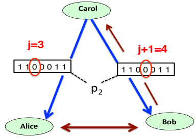
Feynman Feyns proposed the following example in order to demonstrate the impossibility of imitating quantum physics by purely classical means. Alice (A) and Bob (B) are given each a spin-1/2 particle of a pair produced in an entangled state
| (1) |
by a remote source operated by Carol (C). (Here are the spin states of Alice’s or Bob’s particle, polarised up (down) the -axis.) Both make accurate spin measurements along the axis making angles (Alice) and (Bob) with the -axis in the -plane. There are four possible outcomes, with each spin pointing either up () or down () their respective axis. An elementary quantum calculation shows that the corresponding joint probabilities are given by
| (2) | |||
The point of the exercise is to demonstrate that the statistics in Eq.(2) are inconsistent with the assumption that particles arrive to Alice and Bob in pre-determine spin states, which then uniquely determine the outcome of each individual measurement. To do so, it is sufficient to consider only seven possible angles , which Alice will choose randomly, with equal probabilities. With Bob always measuring at , the probability to have the same result is
| (3) |
To prove the point, we assume that, in the classical version of the experiment, Carol sends Alice and Bob the same instruction, containing a -digit strings of ’s and ’s. With the results of all possible measurements now pre-determined,
Alice randomly chooses the -th position in her string, , which corresponds to measuring her spin at .
Then she and Bob read the -th and -th entries, respectively, and count the number of cases, , in which their
results coincide. After trials, the ratio gives a good approximation to the classical probability .
The question is whether Carol can achieve , as would be the case in the quantum version of the game.
Not all instructions are, however, admissible. In the quantum case, Bob measuring at ,
will always disagree with Alice, since from Eq.(2) we have .
To mimic this in the classical case, we must ensure that the entries at the -th and -d positions disagree as well.
This leaves Carol with only eight possible strings, which she can send with the probabilities
, , ,
| (4) | |||
Equations (4) define a simple statistical ensemble with eight possible states (instructions), each endowed with the corresponding probability. Carol’s task is now to find a suitable set of ’s, such that A and B will have the same result with a
probability given by Eq.(3).
This, however turns out to be impossible. The best rate of coincidences
is achieved if Carol sends only the instruction(s) with the largest possible number of agreements, , between a digit and its neighbour to the right. Such are the states and in Eqs.(4),
for which we have . With Alice choosing her entry randomly, the classical probability for her and Bob’s results to coincide is limited by
| (5) |
Disagreement with the correct quantum result (3) is evident, so the classical simulation must fail.
III Compatibility test. Negative probability.
We are not interested in merely repeating the argument of Feyns , and will go one step further, to look at the kind of difficulties which would occur, should we try to reconcile the probabilities in (4) with those in Eq.(2). Consider first states , and a corresponding set of probabilities, , There is also a set of known real functions , . Alice, in her new role, evaluates the averages
| (6) |
by sampling an according to the distribution , writing down , adding up all the results,
and dividing the sum by the number of trials. In doing so, Alice may use the same distribution
or, perhaps, choose a different one, for some of the . Given the values of , we wish to know whether Alice
could have used the same distribution for all her averages, or had to apply a different one at least once.
To answer this question we need to examine linear equations,
| (7) | |||
in order to see if they admit nonnegative solutions .
If they do, Alice could have used the for all . If not, some of the averages must
correspond to a different statistical ensemble. We will call results incompatible,
if one or more different ensembles are required for their preparation.
A trivial example is the case , , . If the averages, suppled by Alice,
are and , equations (7) have no solutions.
Thus, we
conclude that Alice must have used , when averaging , and a different
for averaging .
Another example involves , , , and .
If Alice supplies the values and , Eqs.(7) have a unique, yet unsuitable, solution
| (8) |
With , Alice would not be able to realise the ensemble (8) in practice Feyns . Thus, we must conclude that she had to use the set when experimenting with , and a different set , when averaging . In the following we will use this simple test in order to establish whether different results of quantum measurements may or may not correspond to the same classical statistical ensemble.
IV Different ensembles and non-locality
Next we return to the example of Sect.II, and examine it in more detail. The probabilities of Alice and Bob obtaining the same results when measuring at and , respectively, can be written as the averages,
| (9) |
where
| (10) |
Equating to the quantum result yields Eqs. (7) in the form
| (11) | |||
It is readily seen that the quantum results at and are compatible, and can be simulated classically, e.g., by choosing
| (12) |
as a valid solution of the first three equations in (11).
It is, however, impossible to find a set
, , which would satisfy all four equations in (11). Indeed,
adding the last three equations, and subtracting the result from the first one, we have .
We can, however, reproduce quantum results classically, if we change the rules of the experiment.
To do so, Bob would only need to inform Carol
that a measurement at is to be performed next, and the ’s in (12) that were suitable
for and
must be changed to some s, which would give the correct results for . In other words, Carol would need to be told when to use a different statistical ensemble (4).
The peculiarity of the quantum case is in the fact that Alice and Bob are able achieve the same result
locally, by agreeing only between themselves the angles for their respective measurements. There is no need for a direct communication with the Carol, since that task appears to be taken care of by the non-local quantum correlations implied by the entangled state (1).
In summary, it is possible for different sets of quantum measurements to produce incompatible averages, By the same token, we must conclude that at least two different statistical ensembles were used in their production. Such ensembles cannot pre-exist the measurements, and are instead fabricated (constructed, shaped) by the interaction with the meters, monitoring the system.
V The making of an ensemble
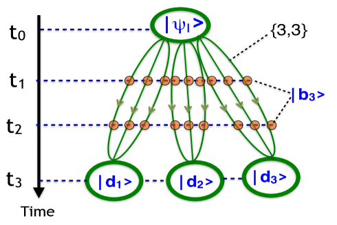
To see how a statistical ensemble can be produced in practice, consider a quantum system with a Hamiltonian , in an -dimensional Hilbert space, prepared in an initial state at some . Suppose we want to accurately measure, at three different times, , three operators , and , with the eigenstates , and , . Out of the eigenvalues , and , only , , have different values, which we will distinguish by means of a subscript, e.g., , . Thus, we can write as
| (13) |
where for and otherwise, and is a projector onto the subspace,
corresponding to the eigenvalue . The operators do not necessarily commute, and
the bases , and are, in general, different.
The measurements will be instantaneous ones, performed by three von Neumann pointers (for details see Appendix A), whose positions are , and ,
respectively. The pointers are prepared in the states , , such that
| (14) |
where is the Dirac delta.
Thus, just after all three meters have fired, the state of the composite system is given by
| (15) | |||
where is the system’s evolution operator.
In the end we examine the positions of all three pointers.
Our choice of measurements defines a statistical ensemble. There are at most possible outcomes (), occurring with the probabilities
, defined by
| (16) | |||
Our aim is to write the probabilities in terms of the corresponding probability amplitudes. Let be the amplitude for "reaching the state at by passing first through the state at , and then through the state at ",
| (17) |
From these we can construct the amplitudes for "reaching a state at by passing through sub-spaces at and at ",
| (18) |
Then for in Eq.(16) we have
| (19) |
where
| (20) |
is the probability of "reaching a state at by passing through sub-spaces at and at "
Equations (19) and (20) are our main result so far. They show that quantum mechanics provides virtual pathways (), connecting with . Each pathway is endowed with a probability amplitude (17), which may or may not be zero. To obtain the probability that in the end the three pointers will point at , , , respectively, we must
(i) add up the amplitudes (17) for passing through all the states corresponding to the degenerate eigenvalues , and .
(ii) add up absolute squares of the results, , summing over all states ,
which correspond to the degenerate eigenvalue .
Thus, the resulting classical ensemble consists of final states, each of which can be reached via at most real pathways, to which we can ascribe both the probabilities , and the amplitudes .
The probabilities add up to unity,
, which is
guaranteed by the unitarity of the evolution of the composite, consisting of the pointers and the measured system.
The net probability to have a value , regardless of what other values might be,
is given by ,
and similarly for .
The quantum origin of the ensemble is evident from the manner in which it was designed and prepared,
Firstly, the observed probabilities must be constructed from probability amplitudes, unknown to classical physics.
Secondly, simply by choosing different degeneracies and we can combine the virtual pathways into different "real" ones, and fabricate different statistical ensembles.
Thirdly, quantum mechanics treats the "present", i.e., the time just after , and the "past", , differently.
To obtain the correct probabilities for and , we add probability amplitudes as in Eq.(18), and take the absolute square of the result. We cannot do the same for by writing as
, and should add the probabilities , as in Eq.(19), instead.
Finally, none of the bases , and are defined uniquely,
unless the eigenvalues of all three operators are non-degenerate, .
Thus choosing different basis vectors to span the orthogonal subspaces, corresponding to degenerate eigenvalues
of , and , would lead to the same observed probabilities (19), yet to different sets of the virtual paths in Eq.(17). These rules are easily generalised to a larger number of intermediate measurements.
In summary, a statistical ensemble,
produced by a series of consecutive measurements, can be described in terms of the real pathways, leading to available final states.
The number of pathways can be increased, by destroying interference between the virtual paths involved,
or decreased, by restoring interference, where it has previously been destroyed. Both tasks can be achieved
by choosing to measure, at intermediate times, different operators, with different numbers of degenerate eigenvalues.
VI A three-state example
To provide a simple illustration, we consider a three-level system, , and limit ourselves to the intermediate measurements of mutually commuting operators, which also commute with the system’s Hamiltonian, . Now and share the same eigenstates, and the Hamiltonian does not allow for transitions between them, since we have . There are, therefore, nine virtual paths shown in Fig. 2, which we will denote by curly brackets, . Omitting, where possible, the subscripts , , and , we write
| (21) |
with the corresponding amplitudes given by [cf. Eq.(17)]
| (22) |
Such a system mimics, for example, the situation of a particle (photon), whose wave packet is split three ways between the wave guides (optical fibres).
Suppose first that, at , we accurately measure an operator with two identical eigenvalues, so that its matrix in the basis is . Then at we measure an operator , which does not commute with , and has non-degenerate eigenvalues . This alone creates six real paths leading to three different destinations , namely and the superpositions (unions) , so that the probabilities of the outcomes are given by
| (23) | |||
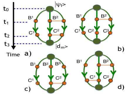
Now at we can measure any operator , with , , without altering the ensemble, already specified by the measurements of and (see Fig. 3a). The only two possible outcomes, shown in Fig.4a will occur with the probabilities given by Eq.(20)
| (24) | |||
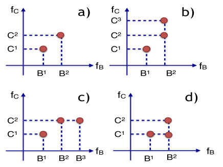
The ensemble, however, will not remain the same if at we decide to measure instead a with (see Fig. 3b). In this case, all nine virtual paths will be made real, and the three possible results shown in Fig. 4b will occur with the probabilities
| (25) | |||
If is measured before (see Fig. 3c), the three outcomes shown in Fig.4c, will occur with probabilities
| (26) | |||
With interference between the paths in Eq.(21) already destroyed by the measurement of ,
measuring of does not modify the ensemble.
Obtaining the net probability for having outcomes and reduces to ignoring the information about the value
of , which is available in principle FeynL . Thus, ,
and not , as would be the case, if were measured on its own.
Finally, joint measurement of at and ,
at also produces nine real paths, even though, on its own, each of the two measurements is capable of producing only one pair of such paths. Indeed, as shown in Figs 3d and 4d, obtaining results , and , will confine the system to the path , obtaining
, and to the path , and obtaining , and to the path .
A similar analysis is easily extended to systems in a Hilbert space of arbitrary number of dimensions , at to intermediate measurements of more than two operators.
VII Non-perturbing measurements, and the reality of the "real" pathways
Previously, we emphasised the difference between virtual paths, endowed only with probability amplitudes, and the
real paths, to which it is also possible to ascribe probabilities.
It is usually accepted that if a measurement of an operator yields the same non-degenerate eigenvalue
in all identical trails, than the system is (or can be said to be) in the corresponding eigenstate .
There is a particular class of non-perturbing ("non-demolition" Real1 ) measurements, which, if applied in addition to the ones being made, leave the statistical ensemble intact,
and only confirm that the system has travelled its particular real pathway.
As a simple example, we choose a basis , , in the Hilbert space of the system, such that it contains its initial state,
. We also choose the three measured operators to be
| (27) |
where is some operator with non-degenerate eigenvalues,
| (28) |
Now the results of all three measurements will aways yield , indicating that the system is in the state , at , . We can add more of such measurements at times between and , all confirming that the system was following its orbit in the Hilbert space,
| (29) |
Recalling the much quoted Einstein’s maxim Real2
"if, without in any way disturbing a system, we can predict with certainty (i.e., with probability equal to unity) the value of a physical quantity, then there exists an element of reality corresponding to that quantity",
we can also conclude that the system really was in the state at any between and .
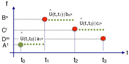
A slightly more interesting case would involve arbitrary operators , and with non-degenerate eigenvalues, and a particular outcome
, corresponding to a real pathway . The pathway is defined only for , and , but we can fill the gaps using the procedure outlined above.
Thus, measuring
| (30) | |||
for a , and , respectively,
will yield only the values , , and , and, therefore, find the system in the states
, and , as shown in Fig. 5.
None of these additional measurements will disturb the original statistical ensemble, and leave the probabilities in Eq.(20) unchanged.
We will not dwell here on the problem of wave function collapse Real3 , evident from the discontinuities in the graph if Fig. 5. It is sufficient to note that whenever the results of the measurements of , and are
(larger dots in Fig. 5),
we can also ascertain (with probability equal to one, and without disturbing the system)
that the system follows a pathway in Fig. 5,
| (31) |
This is the most complete description of a real path, which connects with , and is produced by
intermediate measurements of and .
The argument is readily extended to the case where in Eq.(13) has degenerate eigenvalues. If so, obtaining , would guarantee that for a the system is in the state
, which can be verified, e.g., by measuring the projector
.
In summary, additional measurements, which can be performed on an existing ensemble fall into two categories . Perturbing, or ensemble forming, measurements produce new real pathways, and fabricate a different ensemble, in general completely distinct from the one we had before. Such measurements do not occur in a classical theory, where it is always assumed that observations should have no effect on the monitored system. Non-perturbing measurements, on the other hand, allow one to confirm additional properties of the system Real1 , without modifying the existing ensemble. With respect to such measurements, the situation is similar to the one in classical physics, where the system’s evolution, interrupted by random events, can be monitored without altering its course. Next we take a closer look at some of the "quantum paradoxes", recently discussed in the literature.
VIII The "three-box paradox"
The simplest example of a quantum mechanical "paradox" is the three-box case 3Ba - 3Bc . A -state system, similar to the one discussed in Sect.VI, can reach a final state, from some , by passing through one of the orthogonal states, , . There are three virtual paths,
| (32) |
and three probability amplitudes (for simplicity we put ) . Allegedly, a paradox arises if the initial, , final, , and intermediate, , states are chosen in such a way that
| (33) |

With no measurements made, the system arrives at with a probability .
A measurement of an operator , leaves the probability unchanged,
and always yields the value . According to the "eigenvalue-eigenstate correspondence"
described at the beginning of Sect. VII, this means that the system always takes the path .
By the same token, measurement of an operator will reveal that
the system always takes the path .
The authors of 3Bb suggest that "a paradox . . . is that at a particular time . . . a particle is in some sense both with certainty in one box, and with certainty in another box". The claim is, however, unwarranted.
Measurements of and , both create ensembles with two real paths (see Figs. 6a and 6b), but the ensembles are incompatible. As in Sect III., there are no probabilities and , which would yield correct average values for both
and , since equations
| (34) |
have no solutions. The system does take paths and with certainty, but this happens in two different circumstances,
created by different measurements.
We can illustrate this by employing non-perturbing measurements of Sect. VII. In the first case, non-perturbing would be the measurements of
projectors , and , before and after the measurement of ,
respectively. They would confirm that at all times the system follows a path .
Similar measurements of , and ,
would confirm that the system always follows different path, , if is measured.
In both cases, an attempt to probe the structure of the real paths further, e.g., by measuring also an operator
with all different eigenvalues, would destroy the existing ensemble, create three real paths,
shown in Fig. 6c, and increase the probability to arrive at from to .
In summary, the authors of 3Ba - 3Bc compare the results corresponding to different
physical conditions, and have no reason to claim a paradox. A person can be certainly at work on a Monday, or at home if this Monday turns out to be a holiday. Since each Monday is ether a workday, or a holiday, there is no need
to be in two places at the same time.
IX Photon’s past in the "nested interferometer"
Our next example is a network of optical fibres and beam splitters () shown in Fig. 7a.
At the point , a photon in injected in a wave packet state and ends up being split into three final states, , , leaving system in three different ways, as shown in Fig. 7.
The system is tuned in such a way that no part of the wave function travels through the fibre (dashed), and we are interested in detecting the photon
by means of a detector . The subject of the ongoing discussion, often touching on the topic of "weak measurements" (WM), is the past of the detected photon Nest1 -Nest6 . We will briefly return to the WM in Sect. XIII, and study first what would happen
if its presence in one of the branches of the interferometer were ascertained by means of accurate "strong" intermediate measurements.
In the absence of such measurements there are three virtual paths leading to the desired outcome,
| (35) | |||
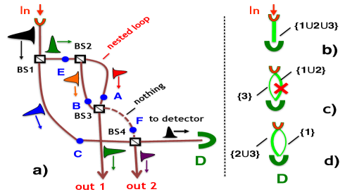
with the probability amplitudes , , and we can proceed as in the previous Section. Paths and are merged together before the and after the , and we can describe detection of the photon at as a measurement of an operator
| (36) |
which does not distinguish between these paths. Detection of a photon at the point may then correspond to measuring an operator
| (37) |
To ensure that no part of the wave function passes through , we must have
| (38) |
together with , which would allow to click occasionally.
Then, an attempt to determine whether the photon passes through would create an ensemble with two real pathways,
the path , travelled with a probability , and
the union (superposition) , never travelled, since .
Note that we can add another such meter at , which would not perturb the system, and merely confirm what has just been said.
A similar situation is shown if Fig. 3a.
Measuring at the operator in Eq.(37)
would create real pathways , and travelled with the probabilities
and .
The same will be true if we try to detect the photon at , by measuring a .
The photon
will be found there with a probability , and detected at with a probability
.
Finally, installing meters both at and , will turn all three paths (35) into real pathways,
labelled by three possible outcomes (cf. Figs. 3d and 4d)
as , and
, and travelled with the probabilities , and , respectively.
The same effect can also be achieved in a different way, for example, by placing meters at both and ,
or at both and .
One may (although by no means needs to) find it strange that the meters at and see no photons,
whereas a meter at or can find one there. This could be elevated to a "paradox" of finding that the photons
"…have been inside the nested interferometer [loop]…, but they never entered and never left the nested interferometer…" Nest2 , but only if this happened within the same statistical ensemble,
i.e., if it were possible o assign non-negative probabilities to the three paths in Eqs.(35).
However, the compatibility test fails, just as in the previous Section, and indicates that the conflicting results correspond to two different ensembles, produced by different sets of measurements. There is no contradiction between having a room full of people, and a room no one can possibly enter, as long as these are two different rooms.
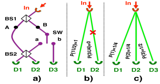
X Interaction-free measurements and the double-slit experiment
So far, we have looked at the examples where the added intermediate measurements destroyed interference between virtual paths, or recombined them, to produce different real pathways. Another way to create a different ensemble would be to provide new final states for the system, and redirect to them some of the existing paths. Consider, for example, the set up in Fig. 7a consisting of two fibres, two beamsplitters, and , and three detectors, , and . There is a switch () which, if set to position , would redirect towards detector a photon, otherwise destined for . The system is tuned is such a way that with set to , the photon always arrives in , and never in . With the switch in this position, there are two virtual paths,
| (39) | |||
leading to , and another two,
| (40) | |||
leading to . The corresponding amplitudes are , , , and . Two real pathways, and , travelled with the probabilities and , lead to two alternative outcomes (see Fig. 8b). To ensure that never clicks, we may choose
| (41) |
one particular choice being , , and IFMsplit .
With the switch in position , there are three possible destinations, , and , reached via real pathways,
| (42) | |||
with amplitudes , , and , travelled with probabilities , and , respectively (see Fig. 8b).
An effect, similar to the one caused by setting the switch to , can be achieved by replacing the switch with an additional system
(a "bomb" in the more colourful language of Eliezur and Vaidman IFM1 ) whose internal state would certainly
change (the bomb would explode) if the photon passes through in Fig. 8a.
This would also affect the destructive interference which prevents the photons from reaching ,
and allow the detector to click occasionally.
What could be considered a "paradoxical" aspect of these experiments, is that the photon can now arrive at only through the left arm of the setup in Fig. 8a,
and is, therefore, capable of detecting the "bomb" in the other arm without interacting with it. Hence,
the term "interaction free measurement" often used in the literature,
for example, in IFM2 ), where a clever application of the Zeno effect allowed the authors to make the maesurement almost
efficient.
The effect itself is not new. One might as well consider a detector placed at the dark (no electrons) fringe of a
Young’s double slit experiment, which starts detecting electrons if one of the slits is blocked. As early as in 1935
Bohr used this example to argue that, in the presence of interference, the idea of a particle passing through
one of the holes must be wrong. In IFMBohr one reads
"If we only imagine the possibility that without disturbing the phenomena we determine through which hole the electron passes, we would truly find ourselves in irrational territory, for this would put us in a situation in which an electron, which might be said to pass through this hole, would be affected by the circumstance of whether this [other] hole was open or closed…"
Similarly one may wonder
how can the photon, arriving at , know that is set to , if it has never paid a visit there?
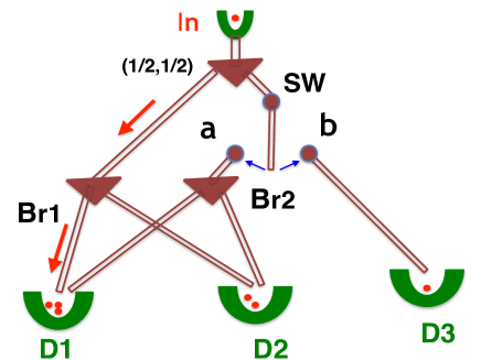
Here we want to look at the problem from a slightly different angle, namely, by considering a classical setup
performing the same function as the quantum one, and try to pinpoint the principle differences between the two.
A classical model shown in Fig. 9 consist of conduits, directing a classical particle (a ball) inserted from the top, towards one of the three receptacles , and .
The triangles in Fig. 9 represent branching connectors, which, if set in a state
, randomly direct a ball, introduced from above, to the left and right conduits, with adjustable probabilities and , respectively. The top connector is always set to , and there is also a switch , whose function is similar to that of the switch in Fig. 8a.
The statistics will be collected by counting the balls ending up in different receptacles , , and .
With the switch in Fig. 9 set to , and and both set to the classical statistics will be the same
as in the quantum case in Fig. 8a with the set to . With the switch in Fig. 8 changed to , and set to , we reproduce the quantum case with set to .
The similarities are obvious. In both cases we much change configuration of the setup. There is no problem with a classical ball rolling into without consulting first
the position of the switch. Arguably, there should not be one with the electron either.
The principle difference is in how the changes can be made. While in the quantum case
single operation on the switch is sufficient, in the classical case we much effect changes in two different, possibly distant, parts of the setup, and . Thus, quantum mechanics allows one to achieve with a single local operation, what classically requires at least two operations in different places. This is a consequence of quantum non-locality, which is well known to forbid considering individual states of an entangled pair IFMent . In the same sense, it forbids separate consideration of the branches of the interferometer in Fig. 8a, through which individual parts of the photon’s wave packet
must propagate before the photon reaches its destination.
XI Composite systems. The Hardy’s "paradox"
Analysis of Sect. V remains valid when we deal with a composite system , consisting
of two sub-systems, and , which exist in and -dimensional Hilbert spaces, respectively.
There are basis states, e.g., direct products each sub-system’s basis functions, and
a typical operator is represented by an matrix.
The setup which could be used for observing the so-called "Hardy’s paradox" HARDY1 ; HARDY2 ; HARDY3 ; HARDY4 is shown in Fig. 10a.
It consists of two systems, each containing two wave guides, two beam splitters, and two detectors.
The inner waveguides approach each other at in such a way that, although unable to jump between the waveguides,
the particles may interact.
Thus, the presence of one particle near in one of the wave guides, may block the passage of the remaining particle through the other wave guide.
For the sake of the argument, one can assume that if a particle and its anti-particle are injected into the left and right subsystem, their encounter
in the vicinity of would result in mutual annihilation, in which case none of the detectors will click,
and a pair of quanta will be observed instead.
The system is tuned in such a way that injection of two non-interacting particles always results in the detections
by detectors in and , while and never click.
The property of interest is that, with the annihilation possible, there is finite probability for and to click simultaneously. This cannot be a result of annihilation, because there would be no particles to arrive
at and . Yet, without the possibility of annihilation, the two detectors would not be able to click.
Our detailed analysis of possible measurements in the Hardy’s
setup can be found in HARDY4 , and here we limit ourselves to a much shorter discussion of its essential features.
Without annihilation,
there are, in principle, four possible outcomes which we denote
, , and , each of which can be reached from the initial state
of two non-interacting particles, , via four virtual paths. For example, four such paths lead to the outcome of interest, [ indicates that the first and the second particles pass through
and , etc.],
| (43) | |||
Together they form a single real pathway, travelled with a probability
| (44) |
Given the symmetry of the setup in Fig. 10a, and the fact that and never click together, for the amplitudes we should have
| (45) |
where is some complex number.
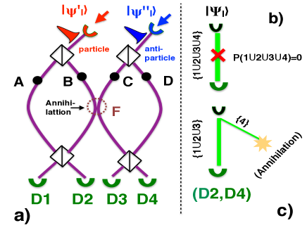
With the annihilation possible, there are only three virtual paths leading to the outcome ,
| (46) | |||
which together form a single real pathways travelled with a probability
| (47) | |||
The fourth path now leads to a different observable outcome,
| (48) |
and is a real pathways in its own right.
Note the similarity with the case of interaction-free measurement, discussed in the previous Section.
As in Sect. X, one of the paths of the composite system (particle-antiparticle pair) is diverted to a different
destination (annihilation), and becomes a new real pathway.
Three remaining virtual paths continue to form a real pathway, but their amplitudes no longer add up to zero,
so that and are able to click in unison.
It is easy to evaluate the probability of joint detection vy and from general considerations.
Let be the amplitude for the first particle to reach via
, and
by symmetry, also the amplitude to reach via .
Since always clicks, if only the first particle is introduced,
we have , or .
By symmetry, is also the amplitude
for the second particle to reach via .
The amplitudes
for independent events multiply FeynL , so that .
Thus, the possibility annihilation allows and to click simultaneously.
From Eq. (47), the probability of this to happen is .
It is a simple matter to evaluate also the probabilities for the remaining four outcomes.
With the diversion of the fourth path to annihilation, the amplitude for and to click
is reduced by one quarter, so that we have . In a similar manner, we conclude that
. This leaves a probability for the annihilation to occur.
We can also check our calculation by evaluating directly. Upon passing a beamsplitter each
wave packet is reduced by a factor of , and the reflected one acquires an additional
phase of . Thus, the norm of the part of the wave function passing through and
is , which is also the probability for the pair to annihilate.
Once again a possible contradiction is avoided by noting that the results and
refer to different statistical ensembles. As in Sect. VIII the compatibility test is trivial.
The condition frustrates any attempts to ascribe
non-negative probabilities , to the virtual paths in Eq.(43).
The uniquely quantum manner in which a new ensemble may be fabricated by introducing
nothing more than a possibility of annihilation, remains the only "paradoxical" feature of the experiment.
XII Composite systems. The "quantum Cheshire cat"
Our last example involves the so called "quantum Cheshire cat" model CAT1 , CAT2
still discussed in the literature CAT3 . The authors of CAT3 suggested that
"most of the works criticizing the effect did not introduce a proper framework in order to
analyze the issue of spatial separation of a quantum particle from one of its properties",
so we take another look at the problem.
Our more detailed
analysis can be found in CAT4 , CAT5 , and here we will discuss a minimalist version of the model,
which captures its essential properties.
Consider a composite, consisting of two two-level systems, and ,
whose basis states are and , , respectively. The full basis consists of four states,
which we can choose to be the products . We expand an arbitrary state of the composite as
,
thus representing it
by a vector ), . We will need two commuting operators,
| (49) |
and
| (50) |
(The authors of CAT1 used a slightly different operator, but
is all we need for our analysis).
Consider first the measurements with no post-selection made.
Suppose we make measurements of on a system prepared in the
same state . A result "1" will then be obtained with a probability
| (51) |
or in approximately trials. If instead we decide to measure , the result "1" will occur with a probability
| (52) |
It is readily seen that if measuring will yield "1" with certainty, , measuring will only yield zeros, ,
| (53) |
Obtaining a result "1" while measuring means that and have been found
in the states and , respectively. Obtaining a "1" while measuring means that
has been found in , regardless of where might have been at the time.
It is not unreasonable, therefore, to interpret Eq.(53) as a proof that
a system cannot "be found with certainty in two places (two orthogonal states) at the same time".
Next we ask what would change if the same measurements are to be made on a system later found (post-selected)
in some state ? It was already mentioned in Sect. V that the past and present of a quantum system
have to be treated differently.
In particular, passing through orthogonal states in the past does not, as such, constitute exclusive alternatives.
Let the system make a transition between states and , represented by coefficients
and , respectively. There are four virtual paths, shown in Fig. 11a,
| (54) | |||
with the amplitudes (we put ).
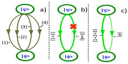
An intermediate measurement of with two degenerate eigenvalues creates two real paths, and (see Fig. 11b), and a result "1" will occur with a probability (we only keep the statistics if the system is found in at the end) . Measuring instead creates paths and (see Fig. 11c), and a result "1" will occur with a probability . Now choosing
| (55) |
(suitable and can always be found CAT4 ) we have
| (56) |
Does this mean that, with post-selection, a particle can "be found with certainty in two places at the same time"? As in all other examples considered above the answer is no. Compatibility test of Sect. III shows that it is not possible to assign meaningful probabilities , to the paths in Eqs.(54) , consistent with Eq.(53). Indeed, the conditions
| (57) | |||
would imply . With the results of two measurements incompatible, we can only make a trivial conclusion. In one setup the final state can be reached via two routes, but one of them is not travelled. In a different setup the same state can be reached by two different routes, such that both are travelled with certain probabilities. Both setups are, in principle, possible.
XIII A note on "weak measurements"
In the previous Sections we discussed the situations which may appear "paradoxical", but cease to be so
once we realise that they refer to different statistical ensembles, produced in a peculiar quantum way,
typically relying on non-local properties of quantum mechanics. The ensembles are not compatible in the sense
that each one requires a different experimental equipment, or different types of particles, and cannot be realised all at one time.
Still, one may suspect that, since all experiments are performed on the same quantum system, different observable properties
must, in some sense, be "present" if the original system is taken in isolation.
The suspicion is correct, and quantum mechanics provides a unique answer. A quantum system in isolation is characterised
by probability amplitudes which can be ascribed to every plausible scenario. The knowledge of the amplitudes by no means implies
that a particular scenario has been realised, rather they suggest what would happen if the
corresponding
equipment
were installed in the lab and turned on. One should not be surprised by the fact that parts and combinations of these amplitudes
can actually be measured in practice, e.g., by studying the response of a system to small perturbations, too weak to
destroy coherence between interfering paths. Elementary perturbation theory routinely uses complex valued off-diagonal
matrix elements of Hermitian operators Bohm , and we may expect something similar to happen, should we decide to use meters which
produce very little disturbance.
One way to minimise the perturbation is to make the initial state of a meter in Eq.(15) to be very broad in the coordinate space, e.g.,
by sending in Eq.(65) of the Appendix A.
The large uncertainty in the initial pointer positions means that the measurement is highly inaccurate.
All ’s in Eq.(15), which are now nearly equal, amount to a common factor
in front of the sums, and the interference between all virtual paths is visibly restored. The problem is that all individual final values of are
now almost equally probable, in accordance with the uncertainty principle FeynL ,
which forbids telling apart interfering alternatives DSann , DSmath .
The averages over many runs of the experiment are, however, well defined.
In the absence of probabilities, these have to be expressed in terms of the amplitudes for the relevant virtual paths.
The rule, re-derived in the Appendix B, is quite simple. If the system is Sect. V passes from a state to some final state ,
and at we make inaccurate intermediate measurements of operators
| (58) |
the mean pointer positions will be given by
| (59) | |||
where
| (60) | |||
is the relative amplitude () for reaching by passing first through the sub-space
. Note that two "weak" pointers are not disturbed by each other’s presence, and is the same, as it would be
if were not measured at all. This situation is typical in perturbation theory, where the first-order effects are always additive.
The complex quantities in the square brackets in Eqs.(59) are nothing but linear combinations of quantum mechanical amplitudes CAT5 .
For example, after many trials, a "weak measurement" of a projector will let us evaluate the real part of the amplitude
and, if projects onto a single state , the real part of the amplitude
for reaching via . Not that the imaginary parts of the can be indirectly
measured in a slightly modified experiment Ah1 , but we are not concerned with them here.
Rather, our purpose is to demonstrate that "weak measurements"
fail to provide a deeper insight into the quantum "paradoxes" mentioned above.
XIII.1 The three-box paradox of Sect. VIII.
Now weak measurements of and would yield the values
| (61) |
But we already know this, for in tuning the system we had to ensure that , or no "paradox" would arise. Hence, no new information is gained. Neither does it mean that the system is "…with certainty in one box, and with certainty in another box" 3Bb . The correct, if less intriguing, statement would be " we checked that the real parts of the (relative) amplitudes for the two virtual pathways are both ".
XIII.2 The nested interferometer of Sect. IX.
Here weak detectors placed at and will let us check previously known [cf. Eq.(38)] relations and . Weak detectors placed only at and , would both yield the real parts of the relative amplitude for the union of the paths and , set to be zero, . The authors of Nest1 and Nest2 chose to conclude that, with no accurate intermediate measurements made, the photon never passed through and , yet "was" in and , so its trajectory must be "discontinuous". Again, this is unwarranted. Their results only confirm the existence of the above relation between the amplitudes for passing via different arms, something the authors of Nest1 and Nest2 must have known when they were building their interferometer.
XIII.3 Hardy’s paradox of Sect. XI.
Here one can employ three commuting projectors , , associated with the three paths in Eqs.(46). Weak measurements of these operators will yield relations between three relative amplitudes , ,
| (62) |
already known from Eq.(45).
The authors of HARDY2 chose to (i) associate with the quantities in Eqs.(60) "the numbers of particle-antiparticle pairs", which pass through a particular route on the way to their respective detectors, and then discuss the meaning of the apparently negative number () of such pairs passing through the outer arms of the interferometer.
It was also argued (ii) that the values in Eqs.(60) "obey a simple, intuitive and, most importantly,
self consistent logic".
We note that (i) is unwarranted. The relative probability amplitudes should not be interpreted as particle numbers.
One would not want to "explain" the two-slit diffraction experiment by saying
that an infinite number of electrons arrive at a dark spot on the screen through one slit, and minus the same number of electrons reach it via the other slit. Furthermore, the statement (ii) is trivial. Relative amplitudes abide by the simple logic obeyed by all probability amplitudes FeynL , plus the additional condition that they should add up to unity.
XIII.4 The quantum Cheshire cat of Sect. XII.
In this case, the relative amplitudes, probed by weak measurements of the operators in Eq.(49) and in Eq.(50), are given by
| (63) |
as one should expect from Eq.(55). This is all an analysis in terms of "weak measurements" can add to our discussion. The authors of CAT1 chose instead to speak about "separation of a particle from its properties",
and we leave it to the reader to decide whether Eqs.(63) warrant such an interpretation.
Finally, we emphasise the circular nature of the argument in all of the above examples. A system is tuned so as to ensure cancellation between certain amplitudes. Then weak measurements are invoked to demonstrate that the amplitudes do indeed have the
desired properties. Calling amplitudes "weak values" does no particular harm, although adds little to the discussion.
Expecting them to be more than just amplitudes, is likely to lead to confusion, and ought to be avoided.
XIV Conclusions and discussion
Our main purpose was to look for a straightforward description of a quantum system subjected to several intermediate measurements. and here we present our findings.
Accurate measurements in a finite-dimensional Hilbert space produce sequences of discrete outcomes, given by the eigenvalues of the measured operators. Thus, the result is a classical statistical ensemble,
specified by the initial and final states of the system, the "real" pathways which connect these states, and the probabilities
with which the pathways are taken. Different sets of measurements "fabricate" different ensembles, which may have little in common, except for the quantum system used in their production.
The uniquely quantum nature of the problem is evident from the manner in which an ensemble is produced,
since the observed real pathways can only be constructed after referring first to the virtual paths of the unobserved system. As a rule, there are many virtual paths, and the relevant ones are selected by the measurements which are to be made. An accurate intermediate measurement then destroys interference between virtual paths to a degree which depends
on the degeneracy of the eigenvalues of the measured operators.
For a given number of intermediate measurements, the maximum number of real pathways, and the most detailed (fine-grained) ensemble, are produced when all eigenvalues are distinct. A less detailed (coarse-grained) ensemble with fewer possible outcomes results from measuring operators
with degenerate eigenvalues.
Typically, a less detailed ensemble cannot be produced from the most detailed one by classical coarse-graining, i.e., by simply adding the probabilities wherever the eigenvalues turn out to be identical.
A simple compatibility test can often be used to demonstrate that, in order to yield the correct coarse-grained probabilities,
some of the fine-grained probabilities would have to be negative, and a suitable fine-grained classical ensemble simply does not exist.
This can be seen as a generalisation of the well known principle, which states that the results of a single quantum measurement
cannot be pre-determined, and are produced in the course of the measurement.
Coarse graining must, therefore, occur via uniting virtual pathways, and adding their amplitudes, rather than probabilities.
Since amplitudes may have opposite signs, the union of two paths may have a zero probability, even though both paths
would be travelled if interference between them were destroyed. Such is, for example, the case of a photon arriving,
after one slit has been blocked,
at the (formerly) dark spot of the interference pattern.
This uniquely quantum feature allows one to produce essentially different statistical
ensembles from the same quantum system, and makes the results of different sets of measurements incompatible,
as discussed in Sect. III.
Another important distinction between fabrication of an ensemble by purely classical and by quantum means,
is the use of non-locality inherent in quantum mechanics. It can be possible to make a classical stochastic system which would reproduce the probabilities of quantum measurements. It can be possible to alter it, in order
for it to mimic a different choice of quantum measurements. However, where an alteration may require several changes made at different locations of the classical setup, fewer modifications could suffice in the quantum case.
For example, what would require flipping the switch and resetting the connector in Fig. 9, can be achieved by simply flipping the switch in Fig. 8.
The layout of the real pathways does not aways coincide with the physical layout of the system.
Thus, in the absence of intermediate measurements, different arms of interferometer in Fig. 7a are, in fact, virtual paths, and the only real pathway via which a photon can reach the detector is their superposition shown in Fig. 7b.
Similarly, in the Hardy’s example, the system in Fig. 10a consists of four distinct wave guides, while the virtual paths of interest
are described in Eqs. (43).
With the path out of the game, the remaining three interfere to
produce a single real pathway in Fig. 10c, thus enabling detection by both and .
There is one aspect in which a quantum-made ensemble resembles a purely classical one.
For a chosen set of "ensemble forming" measurements, there exist other "non-perturbing" measurements which, if added, will not alter the original probabilities, create new real pathways, or change the system’s possible destinations. Unique values, obtained in such measurements, play the role of the pre-existing values of classical physics. With non-perturbing measurements, and only with them, the situation is indeed classical,
and observation without disturbing is possible. For example, in the Hardy’s case,
detectors designed to distinguish between the path leading to annihilation, and the paths , and ,
but not between , and individually, could be installed at several locations along the wave guides.
All detectors would click without fail, whenever the pair of particles is detected by and , which would still happen
with the probability .
It is in this sense that the pathway uniting the three virtual paths in Eq.(46)
can be considered real.
A yet more detailed analysis, desirable as though may seem, encounter a serious difficulty.
The wave guides, which to us are three different objects, appear but a single conduit for the particle-antiparticle pair. Is it possible to peek inside this "real path",
and see what actually happens in different arms of the setup shown in Fig. 10a?
The uncertainty principle says no DSmath ,
and in trying to answer the "which way?" question we meet with a familiar dilemma FeynL .
Installing one or more accurate detectors
would tell which way the pair has travelled, but would also change the probability of detection by and from
to , thus leaving us with a different ensemble.
Making the detectors as delicate as possible helps to avoid the perturbation,
but only reveals relations between probability amplitudes, in principle already known to us.
We ask "what can be said about individual virtual paths?" and receive,
in an operational way, the textbook answer "probability amplitudes".
Finally, the recipe for evaluating frequencies of observed events by finding first the amplitudes of all
relevant virtual scenarios, adding them up, as appropriate, and then taking the absolute squares
is by no means new. It can be found in the first chapter of Feynman’s undergraduate text FeynL .
Above we only outlined a particular way to define the scenarios, which may occur in consecutive measurements, and the rules for adding their amplitudes.
Our conclusions may seem, therefore, to point towards the
"Shut up an calculate!" attitude, famously articulated by David Mermin Merm2 .
Could we have done better, for example, by providing a yet deeper insight into why the measurements outcomes
are random, and why is it necessary to deal with complex valued probability amplitudes, before the probabilities of the outcomes can even be evaluated? Probably not.
We conclude with Feynman’s advice to his undergraduate audience FeynL :
So at the present time we must limit ourselves to computing probabilities. We say "at the present time", but we suspect very strongly that it is something to be with us forever…- that this is the way nature really is.
XV Appendix A. Accurate ("Strong") impulsive von Neumann measurements
An impulsive von Neumann measurement Real3 of an operator at entangles the state of the measured system, , with the position of a pointer, ,
by means of an interaction Hamiltonian .
Initially, the state of the composite system+meter, , is the product of , and the pointer’s state . With the constant put to unity, immediately after the interaction is transformed into ,
, where . One extracts information about the value of , by accurately determining
the pointer’s final position.
Next consider such measurements, performed at on a system with an evolution operator .
The measured operators need not commute and, for simplicity, we assume their eigenvalues to be non-degenerate. In addition, at the system is found (post-selected) in a state . Performing the measurements one after another, we find the amplitude to have the pointer readings , ,
| (64) | |||
with the corresponding probability given by .
Let all be identical Gaussians of a width ,
| (65) |
For an accurate (strong) measurement we choose , which gives
| (66) |
and, with the help of Eq. (64), for the probability to find pointers readings we obtain
| (67) |
Thus, the average position of the -th pointer is given by,
| (68) |
and for a correlator we find
| (69) |
Clearly, there are real pathways, ,
which the measured system travels with the probabilities . The value of on a pathway
passing through is its eigenvalue .
The approach is easily extended to measurements of operators with degenerate eigenvalues, , where is the projector on the sub-space spanned by the eigenstates, corresponding to
the degenerate eigenvalue . In this case, in Eqs. (64) should be replaced by
, summation over by a sum over , and one-dimensional projectors by .
A useful example is the measurement of a series of one-dimensional projectors, . Now each
has a non-degenerate eigenvalue , and -degenerate eigenvalue , so that . There are real pathways, passing at either through the state , or through the sub-space orthogonal to it. It is easy to see that that
the average in Eq.(69) now coincides with the probability to travel the path passing through at every ,
| (70) |
Finally, in practice it may be more convenient to couple the pointer via its position , rather than through its momentum , and measure its final velocity instead of its final position. With the interaction now reading , a change to the momentum representation (with respect to the pointer) yields . After the interaction with the meter we have , where . A strong accurate measurement now requires a pointer with a well defined initial momentum (a narrow ), and the only other difference is the sign of the shift in the momentum space evident in .
XVI Appendix B. Inaccurate ("weak") impulsive von Neumann measurements
A natural complement to the Appendix A is a brief discussion of the results obtained in the limit where the measurements are made deliberately inaccurate, in order to perturb the observed system as little as possible. In Georg the authors, who studied a similar problem, chose to reduce the couplings between the system and the meters involved. Here we would do it slightly differently, namely by sending in Eq.(65) to infinity, and making the initial position of a meter indeterminate. It is convenient to rewrite Eq.(64) as
| (71) | |||
It is readily seen that
| (72) |
Since integration over is restricted to the finite range, containing the eigenvalues of , and is now broad, we can write
| (73) |
where is a small parameter. Individual pointer positions can now lie almost everywhere, and are of no particular interest DSmath . Whatever information about such a measurement may produce, should be obtained from the average pointer positions, evaluated over many runs of the experiment. Let us see what kind of information can be gained in this way. For , to the leading order in , we have
| (74) | |||
where we have used
| (75) | |||
and Eq.(72). Equation (75) is valid regardless of whether the eigenvalues are degenerate or not. The complex valued quantity in rectangular brackets in Eq.(74) is often called "the weak value of an operator ", which can also be written in an equivalent form (see, e.g., Nest6 )
| (76) |
where is the relative amplitude for reaching via . The weak value (76) is, therefore, a sum of such relative amplitudes, weighted by the eigenvalues of . The weak value of a projector onto a sub-space, , spanned by orthogonal states , ,
| (77) |
is just the sum of the relative amplitudes for all paths ,
| (78) |
Calculation of correlations between positions of several weak pointers is more involved. Using equations (75), we have
| (79) |
For just two weak meters, , Eq.(79) yields
| (80) |
where and are given by Eqs.(76). The second term in Eq.(80), , is the sequential weak value of Georgiev and Cohen Georg
| (81) |
where
is the amplitude to reach via . With both and chosen to be the projectors onto and , respectively, the sequential weak value (81) reduces to the amplitude
, as was argued in Georg . Note, however, that it is not directly proportional to the measured , due to the presence of the extra term in the r.h.s. of Eq.(80).
We finish our discussion of weak measurements by noting the well known fact Ah1 that also imaginary parts of the weak values or, indeed, any real valued combination of their real and imaginary parts DSann , can be measured
by preparing and reading the pointer(s) differently. For example, we can determine the average values of the pointer momenta, , instead of their mean positions. Using
| (82) | |||
we obtain equations similar to Eqs. (74) and (80), but for the imaginary parts of the quantities involved,
| (83) |
and
| (84) |
As in the case of strong measurements (see Appendix A), we could also use a pointer, coupled
to the system via . Then, to make the measurement inaccurate (weak), we would choose its initial
state to have a large uncertainty in the momentum space (a broad ). Now evaluating its mean momentum will allow one to determine the real part of in Eq.(76), while its mean position, , will contain
information about .
The reader who finds the content of this Appendix but a tedious exercise in perturbation theory would be right.
Since weakly perturbing meters do not create new real pathways, there are no probabilities, and their mean readings are expressed in terms of the corresponding probability amplitudes and their weighted combinations, otherwise
known as "weak values".
XVII Acknowledgements
Support by the Basque Government (Grant No. IT986-16), as well as by MINECO and the European Regional Development Fund FEDER, through the grant FIS2015-67161-P (MINECO/FEDER) is gratefully acknowledged.
References
- (1) X. Zhu, Y. Zhang, S. Pang, C. Qiao, Q. Liu, S. Wu, Quantum measurements with preselection and postselection, Phys. Rev. A 84, 052111 (2011).
- (2) Y. Aharonov, L. Vaidman, Complete description of a quantum system at a given time, J. Phys. A 24, 2315 (1991).
- (3) T. Ravon, L. Vaidman, The three-box paradox revisited, J. Phys. A 40, 2873 (2007).
- (4) Y. Aharonov, L. Vaidman, The two-state vector formalism: an updated review, in: J.G. Muga, R. Sala Mayato, I.L. Egusquiza (Eds.), Time in Quantum Mechanics, Springer, (second edition), 2008, p.406.
- (5) D. Sokolovski, I. Puerto Gimenez, R. Sala-Mayato, Path integrals, the ABL rule and the three-box paradox, Phys. Lett. A 372, 6578 (2008).
- (6) L. Vaidman, Past of a quantum particle, Phys. Rev. A 87, 052104 (2013).
- (7) A. Danan, D. Farfurnik, S. Bar-Ad, L. Vaidman, Asking photons where they have been, Phys. Rev. Lett., 111, 240402 (2013).
- (8) P.L. Saldanha, Interpreting a nested Mach-Zehnder interferometer with classical optics, Phys. Rev. A 89, 033825 (2014).
- (9) R.B. Griffiths, Particle path through a nested Mach-Zehnder interferometer, Phys. Rev. A 94, 032115 (2016).
- (10) D. Sokolovski, Asking photons where they have been in plain language, Phys. Lett. A 381, 227 (2014).
- (11) Q. Duprey, A. Matzkin, Null weak values and the past of a quantum particle, Phys. Rev. A 95, 032110 (2017).
- (12) L. Hardy, Quantum mechanics, local realistic theories, and Lorentz-invariant realistic theories, Phys. Rev. Lett., 68, 2981 (1992).
- (13) Y. Aharonov, A. Botero, S. Popescu, B. Reznik, J. Tollaksen, Revisiting Hardy’s paradox: counterfactual statements, real measurements, entanglement and weak values, Phys. Lett. A 301, 130 (2002).
- (14) J.S. Lundeen, A.M. Steinberg, Experimental joint weak measurement on a photon pair as a probe of Hardy’s paradox, Phys. Rev. Lett., 102, 020404 (2009).
- (15) D. Sokolovski, I. Puerto Gimenez, R. Sala-Mayato, Feynman-path analysis of Hardy’s paradox: Measurements and the uncertainty principle, Phys. Lett. A 372, 3784 (2008).
- (16) R.P. Feynman, R. Leighton, M. Sands, The Feynman Lectures on Physics III Dover Publications, Inc., New York, 1989, Ch.1: Quantum Behavior.
- (17) Ya. Aharonov, S. Popescu, D. Rohrlich, P. Skrzypczyk, Quantum cheshire cats, New. J. Phys. 15, 113015, (2013).
- (18) T. Denkmayr, H. Geppert, S. Sponar, H. Lemmel, A. Matzkin, J. Tollaksen, Y. Hasegawa, Observation of a quantum Cheshire Cat in a matter-wave interferometer experiment, Nature. Comm. 5, 4492, (2014).
- (19) D. Sokolovski, The meaning of "anomalous weak values" in quantum and classical theories, Phys. Lett. A 379, 1097 (2015).
- (20) D. Sokolovski, Weak measurements measure probability amplitudes (and very little else), Phys. Lett. A 380, 1593 (2016).
- (21) Q. Duprey, S. Kanjilal, U. Sinha, D. Home, A. Matzkin, The quantum cheshire cat effect: theoretical basis and observational implications, Ann. Phys. 391, 1 (2018).
- (22) H.P. Stapp, Nonlocal character of quantum theory, Am. J. Phys. 65, 300 (1997).
- (23) W. Unruh, Nonlocality, counterfactuals, and quantum mechanics, Phys. Rev. A 59, 126(1997).
- (24) H.P. Stapp, Meaning of counterfactual statements in quantum physics, Am. J. Phys. 66, 924 (1998).
- (25) R.E. Kastner, The three-box "paradox" and other reasons to reject the counterfactual usage of the ABL rule, Found. Phys. 29, 851 (1999).
- (26) D. Sokolovski, E. Akhmatskaya, An even simpler understanding of quantum weak values, Ann. Phys.388, 382 (2018).
- (27) D. Sokolovski, Salecker-Wigner-Peres clock, Feynman paths, and a tunnelling time that should not exist, Phys. Rev. A 96, 022120-1 (2017).
- (28) D. Sokolovski, E. Akhmatskaya, "Superluminal paradox" in wave packet propagation and its quantum mechanical resolution, Ann. Phys. 339, 307 (2013).
- (29) G.C. Knee, K. Kakuyanagi, M.-C. Yeh, Y. Matsuzaki, H. Toida, H. Yamaguchi, S. Saito, A.J. Leggett, W. Munro, A strict experimental test of macroscopic realism in a superconducting flux qubit, Nat. Comm. 7, 13253 (2016).
- (30) A.J. Leggett, A. Garg, Quantum mechanics versus macroscopic realism: is the flux there when nobody looks? Phys. Rev. Lett. 54, 857 (1985).
- (31) C. Emary, N. Lambert, F. Nori, Leggett-Garg inequalities, Prog. Rep. Phys.77, 857 (2013).
- (32) C. Emary, Ambiguous measurements, signaling, and violations of Leggett-Garg inequalities. Phys. Rev. A 96, 042102 (2017).
- (33) J. von Neumann, Mathematical Foundations of Quantum Mechanics, Princeton University Press, Princeton, 1955.
- (34) N.D. Mermin, Hidden variables and the two theorems of John Bell, Rev. Mod. Phys. 65, 803 (1993).
- (35) R.P. Feynman, Simulating physics with computers, Int. J. Theor. Phys. 64, 467 (1982).
- (36) C. Monroe, Demolishing quantum nondemolition, Phys.Today 64 , 8 (2011).
- (37) A. Einstein, B. Podolsky, N. Rosen, Can quantum-mechanical description of physical reality be considered complete? Phys. Rev. 47, 777 (1935).
- (38) A.C. Elitzur, L. Vaidman, Quantum mechanical interaction-free measurements, Found. Phys. A 23, 988 (1993).
- (39) P. Kwiat, H. Weinfurter, T. Herzog, A. Zeilinger, Interaction-free measurement, Phys. Rev. Lett., 74, 4763 (1995).
- (40) R. Loudon, The quantum theory of light, third edition, Oxford University Press, New York, NY, 2000.
- (41) N. Bohr, Space and time in nuclear physics. Ms. 14, March 21, Manuscript Collection, Archive for the History of Quantum Physics, American Philosophical Society, Philadelphia.
- (42) M.A. Nielsen, I.L. Chuang, Quantum Computation and Quantum Information, Cambridge University Press. 2000.
- (43) D. Sokolovski, Quantum measurements, stochastic networks, the uncertainty principle, and the not so strange "weak values". Mathematics 4, 56 (2016) [open access].
- (44) D. Bohm, Quantum Theory, Dover, NY, 1989.
- (45) Y. Aharonov, D.Z. Albert, L.Vaidman, How the result of a measurement of a component of the spin of a spin-1/2 particle can turn out to be 100, Phys. Rev. Lett. 60, 1351 (1988).
- (46) N.D. Mermin, What’s wrong with this pillow? Physics Today 42, 9 (1989).
- (47) D. Georgiev, E. Cohen, Probing finite coarse-grained virtual Feynman histories with sequential weak values, Phys. Rev. A 97, 052101 (2018).