Exponential stabilization of a smart piezoelectric composite beam with only one boundary controller

Abstract

Layered smart composite beams involving a piezoelectric layer are traditionally actuated by a voltage source by the extension mechanism. In this paper, we consider only the bending and shear of a cantilevered piezoelectric smart composite beam modeled by the Mead-Marcus sandwich beam assumptions. Uniform exponential stabilitization with only one boundary state feedback controller, simultaneously controlling both bending moment and shear, is proved by using a spectral multiplier approach. The state feedback controller slightly differs from the classical counterparts by a non-trivial compact and nonnegative integral operator. This is due to the strong coupling of the charge equation with the stretching and bending equations. For simulations, the so-called filtered semi-discrete finite difference scheme is adopted.

1 Introduction

A piezoelectric smart composite beam is a three-layer sandwich beam consisting of a stiff elastic layer, a complaint (viscoelastic) layer, and a piezoelectric layer, see Fig. 1. The piezoelectric layer is also an elastic beam with electrodes at its top and bottom surfaces and connected to an external electric circuit. As the electrodes are subjected to a voltage source, an electric field is created between the electrodes, and the piezoelectric beam shrinks or extends. Therefore, the whole composite stretches and bends (see Fig. 1).

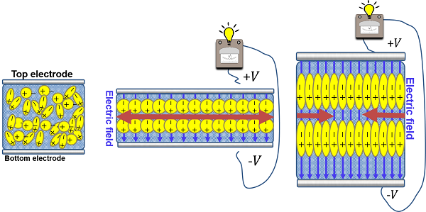
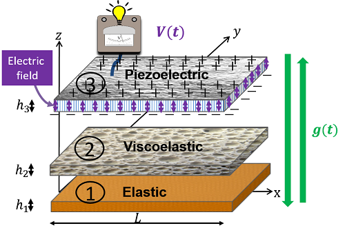
Figure 1: (a) A piezoelectric beam extents or shrinks by supplying voltage to its electrodes since the charges separate and line up in the vertical direction. (b) A voltage-actuated piezoelectric smart composite of length $L$ with thicknesses $h_{1},h_{2},h_{3}$ for its layers ①, ②, ③, respectively. Both voltage $V(t)$ and shear $g(t)$ controller control bending motions on the composite. In fact, it is the goal of the paper that the voltage controller $V(t)$ itself has the ability to control all bending and shear motions on the composite in a few seconds.

The modeling assumptions for smart piezoelectric models can be classified in two main categories: mechanical and electro-magnetic. The mechanical assumptions can be classified in two main categories, i.e. see Trindade and Benjendou (2002): either Mead-Marcus (M-M) type Baz (1997) or Rao-Nakra (R-N) type Baz (1997); Lam et al. (1997). The M-M models only involve the transverse kinetic energy whereas the R-N models involve both longitudinal and transverse kinetic energies. Both types of models reduce to the classical counterparts, see Ozer (2016), once the piezoelectric strain is taken to be zero. The electro-magnetic assumptions on the piezoelectric layer are either fully dynamic, quasi-static, or electrostatic, see Morris and Ozer (2014); Ozer (2015). The electrostatic assumption completely discards electrical and magnetic-kinetic energies due to Maxwell’s equations. It is still a standard assumption in the literature, see Smith (2005). The voltage control, actuating the piezoelectric layer, is simply blended into models through the boundary conditions.

For the passive sandwich beam models (having no piezoelectric layer), the exact controllability of the M-M and R-N models are shown for the clamped and hinged models Hansen and Ozer (2010); Ozer and Hansen (2014). The exponential stability in the existence of the passive damping term due to the shear of the middle layer is investigated for the M-M model (Allen and Hansen (2010); Wang and Guo (2008)) . The active boundary feedback stabilization of the classical R-N model is only investigated for hinged (Ozer and Hansen (2013)) and clamped-free (Wang et al. (2006)) boundary conditions. The exponential stabilizability of the cantilevered fully dynamic or electrostatic M-M and R-N models has been open problems for more than a decade. Note that cantilevered boundary conditions are more physical than clamped or hinged boundary conditions. Recently, the exponential stability of the electrostatic R-N model is shown by using four feedback controllers Ozer-a (2017), two for stretching motions of outer layers, and two for the bending motion. The exponential stability with only three controllers is recently shown by using a spectral-theoretic approach Yang and Wang (2017), and by a higher order spectral multipliers approach (Ozer-a (2017); Ozer-b (2017)). The fully dynamic R-N model is shown to be not stabilizable for many choices of material parameters by using $B^{*}-$type feedback controllers Ozer-a (2017). The charge-actuated electrostatic counterparts are also shown to be exponentially stable in Ozer-a (2018).

To our knowledge, the exponential stabilizability for “cantilevered” fully dynamic or electrostatic M-M model have never been studied in the literature. Denoting stretching of the top and the bottom layers, bending of the composite, shear due to the middle layer, and the total induced charge accumulated at the piezoelectric layer by $v^{1},v^{3},w,\phi^{2},p$ respectively, the equations of motion for the fully dynamic M-M model is obtained in Ozer-b (2017) by a thorough variational approach as the following

$$\left\{\begin{array}[]{ll}m\ddot{w}+Aw_{xxxx}-B_{1}\varsigma\gamma\beta h_{2}h_{3}\phi^{2}_{x}+\gamma\beta B_{3}p_{xxx}=0,&\\ C\varsigma\phi^{2}-\phi^{2}_{xx}+B_{1}w_{xxx}+B_{2}p_{xx}=0,&\\ \mu h_{3}\ddot{p}-B_{4}\beta p_{xx}+\gamma\beta h_{2}h_{3}\varsigma B_{2}\phi^{2}&\\ \quad\quad\quad\quad\quad-\gamma\beta B_{3}w_{xxx}=-V(t)\delta_{L},&\end{array}\right.$$ (5)

$$\left\{\begin{array}[]{ll}\left|w,w_{x},\phi^{2},p~{}\right|_{x=0},\quad\left|w_{xx}=\phi^{2}_{x}=p_{x}\right|_{x=L}=0,&\\ \left|-Aw_{xxx}+B_{1}\varsigma\gamma\beta h_{2}h_{3}\phi^{2}-\gamma\beta B_{3}p_{xx}\right|_{x=L}=g(t).\end{array}\right.$$ (8)

where $\delta_{L}=\delta(x-L)$ is the Dirac-Delta distribution at $x=L,$ $\phi^{2}=\frac{1}{h_{2}}\left(-v^{1}+v^{3}\right)+\frac{H}{h_{2}}w_{x},$ $H=\frac{h_{1}+2h_{2}+h_{3}}{2},$ and $h_{i}$ is the thickness of the ${\rm{i}}^{\rm th}-$ layer, and $\beta,\gamma,\mu>0$ are piezoelectric constants, and
$m,A,B_{1},\ldots,B_{4},C,\varsigma>0$ are functions for material parameters of each layer. Moreover, $V(t)$ is the voltage controller actuating the piezo-layer, and $g(t)$ is actuating the transverse shear mechanism at the tip. The lack of stabilizability of this model for certain sub-classes of solutions is studied in Ozer-b (2017).

Notice that if the electrostatic assumption is adopted, i.e. $\mu h_{3}\ddot{p}\equiv 0,$ the model (8) reduces to

$$\left\{\begin{array}[]{ll}m\ddot{w}+{\tilde{A}}w_{xxxx}-\beta\gamma h_{2}h_{3}\varsigma{\tilde{B}}\phi^{2}_{x}=-\frac{\gamma B_{3}}{B_{4}}V(t)(\delta_{L})_{x},&\\ \varsigma{\tilde{C}}\phi^{2}-\phi^{2}_{xx}+{\tilde{B}}w_{xxx}=-\frac{B_{2}}{\beta B_{4}}V(t)\delta_{L},&\end{array}\right.$$ (11)

$$\left\{\begin{array}[]{ll}w(0)=w_{x}(0)=\phi^{2}(0)=w_{xx}(L)=\phi^{2}_{x}(L)=0,&\\ -\tilde{A}w_{xxx}(L)+\beta\gamma h_{2}h_{3}\varsigma{\tilde{B}}\phi^{2}(L)=g(t)\end{array}\right.$$ (14)

where the coefficients are $\tilde{A}=A-\frac{\gamma^{2}\beta B_{3}^{2}}{B_{4}}>0,\tilde{B}=B_{1}-\frac{\gamma B_{2}B_{3}}{B_{4}}>0,\tilde{C}=C+\frac{\gamma h_{2}h_{3}B_{2}^{2}}{B_{4}},$ see Ozer (2016).

The case $g(t)\neq 0,V(t)=0$ corresponds to the standard (passive) M-M model, and its stabilizability is studied in Wang et al. (2006). To our knowledge, the only stabilizability result for the electrostatic model ($V(t)\neq 0$, $g(t)=0$) is provided by Baz (1997) where various PID-type feedback controllers are considered for the asymptotic stability of the system. These results do not imply the exponential stability whatsoever. In fact, a shear-type of passive damping is also included in their models as the following:

$$\left\{\begin{array}[]{ll}m\ddot{w}+{\tilde{A}}w_{xxxx}-\beta\gamma h_{2}h_{3}\varsigma{\tilde{B}}\phi^{2}_{x}=-\frac{\gamma B_{3}}{B_{4}}V(t)(\delta_{L})_{x},&\\ \kappa\dot{\phi}^{2}+\varsigma{\tilde{C}}\phi^{2}-\phi^{2}_{xx}+{\tilde{B}}w_{xxx}=-\frac{B_{2}}{\beta B_{4}}V(t)\delta_{L}\end{array}\right.$$ (17)

where $\kappa>0$ is the damping coefficient. It is proven in Wang and Guo (2008) that the damping term itself exponentially dissipates the energy of (17), even without the boundary feedback damping: $V(t)\equiv 0$. Hence, it is not clear whether $V(t)$ can be designed to exponentially dissipate the energy by itself.

In this paper, first we show that the the model (14) is well-posed on an appropriate Hilbert space. Next, we prove that the overdetermined problem, with an extra measurement, has only the trivial solution by using spectral multipliers to ensure the strong stability. Without considering the shear-type of passive damping, i.e. $\kappa=0$ in (17), the exponential stability of the electrostatic M-M model is guaranteed by using only the $B^{*}-$type state feedback controller for $V(t)$. The proof combines the a spectral multiplier method and a frequency domain approach as in Liu and Liu (2002). Finally, the so-called filtered semi-discrete Finite Differences is proposed first time to design the approximated stabilizing controller for a strongly coupled system.

2 Well-posedness

Define the operator $(\varsigma\tilde{C}I-D_{x}^{2})$ on the domain $H^{2}_{L}(0,L):=\{\psi\in H^{2}(0,L):\psi_{x}(0)=\psi_{x}(L)=0\}.$ Therefore, the operator $P_{\varsigma}=(\tilde{C}\varsigma I-D_{x}^{2})^{-1}$ is defined by

$$P_{\varsigma}(f)(x)=\int_{0}^{L}g(x,z)f(z)dz,\quad{\rm with}$$ (18)

$$g(x,z)=\left\{\begin{array}[]{ll}\frac{\cosh{[\sqrt{\tilde{C}\varsigma}(z-L)]}\sinh{[\sqrt{\tilde{C}\varsigma}x]}}{\sqrt{\tilde{C}\varsigma}\cosh{[\sqrt{\tilde{C}\varsigma}L]}}&x\leq z\\ \frac{\cosh{[\sqrt{\tilde{C}\varsigma}(x-L)]}\sinh{[\sqrt{\tilde{C}\varsigma}z]}}{\sqrt{\tilde{C}\varsigma}\cosh{[\sqrt{\tilde{C}\varsigma}L]}}&x\geq z.\end{array}\right.$$ (21)

It is well-known that $P_{\varsigma}$ is a compact and non-negative operator on ${\mathbb{L}}^{2}(0,L)$. We have the following result:

Lemma 1.

Let ${\rm Dom}(D_{x}^{2})=H^{2}_{L}(0,L).$ Define the operator $J_{\varsigma}:=\varsigma\tilde{C}P_{\varsigma}-I.$ Then, $J_{\varsigma}$ is continuous, self-adjoint and and non-positive on ${\mathbb{L}}^{2}(0,L).$ Moreover, for all $w\in{\rm Dom}(P_{\varsigma}),$ $J_{\varsigma}w=~{}P_{\varsigma}D_{x}^{2}=(\varsigma\tilde{C}I-D_{x}^{2})^{-1}D_{x}^{2}w.$

Proof: Continuity and self-adjointness easily follow from the definition of $J_{\varsigma}.$ We first prove that $J_{\varsigma}$ is a non-positive operator. Let $u\in{\mathbb{L}}^{2}(0,L).$ Then $P_{\varsigma}u=(\varsigma\tilde{C}I-D_{x}^{2})^{-1}u=s$ implies that $s\in{\rm Dom}(D_{x}^{2})$ and $\varsigma\tilde{C}s-s_{xx}=u$

$$\left<J_{\varsigma}u,u\right>_{{\mathbb{L}}^{2}(0,L)} = \left<(\varsigma\tilde{C}P_{\varsigma}-I)u,u\right>_{{\mathbb{L}}^{2}(0,L)}$$

$$= -\varsigma\tilde{C}\|s_{x}\|^{2}_{{\mathbb{L}}^{2}(0,L)}-\|s_{xx}\|^{2}_{{\mathbb{L}}^{2}(0,L)}.$$

Let $J_{\varsigma}w=(\varsigma\tilde{C}P_{\varsigma}-I)w$ and $v:=P_{\varsigma}w.$ Then $\varsigma\tilde{C}v-v_{xx}=w.$ By a simple rearrangement of the terms

$$J_{\varsigma}w=(\varsigma\tilde{C}v-w)=(\varsigma\tilde{C}v-\varsigma\tilde{C}v+v_{xx})=v_{xx}=P_{\varsigma}D_{x}^{2}w.\square$$

By Lemma 1, (14) can be simplified to

$$\left\{\begin{array}[]{ll}m\ddot{w}+{\tilde{A}}w_{xxxx}+\gamma\beta\varsigma h_{2}h_{3}\tilde{B}^{2}(J_{\varsigma}w_{x})_{x}=&\\ \quad-\frac{\gamma}{B_{4}}\left[\varsigma h_{2}h_{3}\tilde{B}B_{2}(P_{\varsigma}\delta_{L})_{x}+B_{3}(\delta_{L})_{x}\right]V(t),\\ w(0)=w_{x}(0)=w_{xx}(L)=0,&\\ {\tilde{A}}w_{xxx}(L)+\gamma\beta\varsigma h_{2}h_{3}\tilde{B}^{2}J_{\varsigma}w_{x}(L)=g(t).\end{array}\right.$$ (26)

This model fits in the form of the abstract Mead-Marcus beam model obtained in Hansen and Ozer (2010).

Since our beam in nonclassical, we discard the mechanical controller; $g(t)\equiv 0.$ Define $\mathcal{H}=\mathrm{V}\times\mathrm{H}=H^{2}_{L}(0,L)\times{\mathbb{L}}^{2}(0,L).$ The energy associated with (26) is

$$\mathrm{E}=\frac{1}{2}\int_{0}^{L}\left\{m|\dot{w}|^{2}+\tilde{A}|w_{xx}|^{2}-\gamma\beta\varsigma h_{2}h_{3}\tilde{B}^{2}J_{\varsigma}w_{x}\bar{w}_{x}\right\}~{}dx.$$

This motivates the definition of the inner product on $\mathcal{H}:$

$$\left<\left[\begin{array}[]{l}u_{1}\\ u_{2}\end{array}\right],\left[\begin{array}[]{l}v_{1}\\ v_{2}\end{array}\right]\right>_{\mathcal{H}}=\left<u_{2},v_{2}\right>_{\mathrm{H}}+\left<u_{1},v_{1}\right>_{\mathrm{V}}=\int_{0}^{L}\left\{mu_{2}{{\bar{v}}_{2}}\right.$$ (31)

$$\left.+\tilde{A}(u_{2})_{xx}(\bar{v}_{2})_{xx}-\gamma\beta\varsigma h_{2}h_{3}\tilde{B}^{2}(J_{\varsigma}(u_{1})_{x})({\bar{u}}_{1})_{x}\right\}~{}dx.$$

Define the operator $\mathcal{A}:{\text{Dom}}(\mathcal{A})\subset\mathcal{H}\to\mathcal{H}$ where $\mathcal{A}=\left[{\begin{array}[]{*{20}c}0&I\\ \frac{-1}{m}\left(\tilde{A}D_{x}^{4}+\gamma\beta\varsigma h_{2}h_{3}\tilde{B}^{2}D_{x}J_{\varsigma}D_{x}\right)&0\\ \end{array}}\right]$ with

$$\left.\begin{array}[]{ll}{\rm{Dom}}(\mathcal{A})=\{(z_{1},z_{2})\in\mathcal{H},z_{2}\in H^{2}_{L}(0,L),~{}~{}\tilde{A}(z_{1})_{xxx}&\\ +\gamma\beta\varsigma h_{2}h_{3}\tilde{B}^{2}J_{\varsigma}(z_{1})_{x}\in H^{1}(0,L),~{}~{}(z_{1})_{xx}(L)=0&\\ \tilde{A}(z_{1})_{xxx}(L)+\gamma\beta\varsigma h_{2}h_{3}\tilde{B}^{2}J_{\varsigma}(z_{1})(L)=0\}.&\end{array}\right.$$ (35)

Define also the control operator $\mathcal{B}\in\mathcal{L}(\mathbb{C},{\rm Dom}(\mathcal{A})^{\prime})$ by

$$\mathcal{B}=\left[\begin{array}[]{c}0\\ -\frac{\gamma}{mB_{4}}\left[\varsigma h_{2}h_{3}\tilde{B}B_{2}(P_{\varsigma}\delta_{L})_{x}+B_{3}(\delta_{L})_{x}\right]\end{array}\right].$$ (38)

The dual operator $\mathcal{B}^{*}\in\mathcal{L}(\mathcal{H},\mathbb{C})$ is defined by $\mathcal{B}^{*}\Phi=\frac{\gamma}{mB_{4}}\left[\varsigma h_{2}h_{3}\tilde{B}B_{2}(P_{\varsigma}(\Phi_{2})_{x}(L))+B_{3}(\Phi_{2})_{x}(L)\right].$
Choosing the state $\Phi=[w,\dot{w}]^{\rm T},$ the control system (26) with the voltage controller $V(t)$ can be put into the state-space form

$$\dot{\Phi}={\mathcal{A}}\Phi+\mathcal{B}V(t),\quad\Phi(x,0)=\Phi^{0}.$$ (39)

Since the piezoelectric smart beam model is similar to the classical counterpart with the electrostatic assumption, the following results are immediate from (Ozer-b (2017)):

Theorem 2.

For fixed initial data and no applied forces, the solution $(w,p)\in\mathcal{H}$ of (8) converges to the solution of $(w,p)\in\mathcal{H}$ in (26) as $\mu\to 0.$

Theorem 3.

Let $T>0,$ and $V(t)\in{\mathbb{L}}^{2}(0,T).$ For any $\Phi^{0}\in\mathrm{H},$ $\Phi\in C[[0,T];\mathcal{H}]$ and there exists a positive constant $c_{1}(T)$ such that (39) satisfies

$$\|\Phi(T)\|^{2}_{\mathcal{H}} \leq c_{1}(T)\left\{\|\Phi^{0}\|^{2}_{\mathcal{H}}+\|V\|^{2}_{{\mathbb{L}}^{2}(0,T)}\right\}.$$ (40)

3 Uniform Stabilization

For $k_{1}>0,$ we choose the following $B^{*}-$type feedback controller

$$V(t)=-\frac{k_{1}mB_{4}}{\gamma}\mathcal{B}^{*}\Phi$$

$$=-k_{1}\left[\varsigma h_{2}h_{3}\tilde{B}B_{2}(P_{\varsigma}\dot{w}_{x}(L))+B_{3}\dot{w}_{x}(L)\right].$$ (41)

The energy of the system is dissipative and it satisfies

$$\frac{dE(t)}{dt}=\gamma V(t)\left[h_{2}h_{3}\varsigma\tilde{B}(P_{\varsigma}\dot{w}_{x})(L)+\frac{B_{3}}{B_{4}}\dot{w}_{x}(L)\right]$$

$$=-k_{1}\left[\left(h_{2}h_{3}\varsigma\tilde{B}B_{2}P_{\varsigma}+B_{3}I\right)\dot{w}_{x}(L)\right]^{2}\leq 0$$

where $h_{2}h_{3}\varsigma\tilde{B}B_{2}P_{\varsigma}+B_{3}I$ is a non-negative operator.

Observe that $P_{\varsigma}\dot{w}_{x}(L)$ is a PID-type feedback, and it is the total piezoelectric effect due to the coupling of the charge equation to shear and bending at the same time. By Lemma 1, it can also be considered as $P_{\varsigma}\dot{w}_{x}(L)=\frac{1}{\varsigma\tilde{B}\tilde{C}}(-\dot{\phi}^{2}+\tilde{B}\dot{w}_{x})(L).$ This type of representation is helpful to design the controller numerically inSection . Therefore (41) reduces to

$$V(t)=-k_{1}\left[\left(\frac{h_{2}h_{3}\tilde{B}B_{2}}{\tilde{C}}+B_{3}\right)\dot{w}_{x}(L)-\frac{h_{2}h_{3}B_{2}}{\tilde{C}}\dot{\phi}^{2}(L)\right].$$

Now consider the system (39) with the state feedback controller (41):

$$\left\{\begin{array}[]{ll}\dot{\varphi}=\tilde{A}\Phi:=\left({\mathcal{A}}-\frac{k_{1}mB_{4}}{\gamma}\mathcal{B}\mathcal{B}^{*}\right)\Phi,\quad\Phi(x,0)=\Phi^{0}.\end{array}\right.$$ (43)

Theorem 4.

The operator $\tilde{\mathcal{A}}$ defined by (43) is dissipative in $\mathcal{H}.$ Moreover, ${\tilde{\mathcal{A}}}^{-−1}$ exists and is compact on $\mathcal{H}.$ Therefore, $\tilde{\mathcal{A}}$ generates a $C_{0}$-semigroup of contractions on $\mathcal{H}$ and the spectrum $\sigma(\tilde{\mathcal{A}})$ consists of isolated eigenvalues only.

Proof Let $Y\in{\rm Dom}(\tilde{\mathcal{A}}).$ Then

$$\left<\mathcal{A}Y,Y\right>=\left.\left(-\tilde{A}(y_{1})_{xxx}-\gamma\beta\varsigma h_{2}h_{3}\tilde{B}^{2}D_{x}J_{\varsigma}(y_{1})\right)\bar{y}_{2}\right|_{x=0}^{L}$$

$$\quad+\left.\tilde{A}(y_{1})_{xx}(\bar{y}_{2})_{x}\right|_{x=0}^{L}$$

$$\quad+\int_{0}^{L}\left[-\tilde{A}(y_{1})_{xx}(\bar{y}_{2})_{xx}+\gamma\beta\varsigma h_{2}h_{3}\tilde{B}^{2}J_{\varsigma}(y_{1})_{x}(\bar{y}_{2})_{x}\right.$$

$$\quad\left.+\left(\tilde{A}(y_{2})_{xx}(\bar{y}_{1})_{xx}-\gamma\beta\varsigma h_{2}h_{3}\tilde{B}^{2}J_{\varsigma}(y_{2})_{x}(\bar{y}_{1})_{x}\right)\right]~{}dx.$$

Therefore,

$${\rm Re}\left<\tilde{\mathcal{A}}Y,Y\right>=-\left[\left(h_{2}h_{3}\varsigma\tilde{B}B_{2}P_{\varsigma}+B_{3}I\right)(y_{2})_{x}(L)\right]^{2}\leq 0.\quad~{}~{}$$ (44)

Therefore $\tilde{\mathcal{A}}$ is dissipative. If ${\tilde{\mathcal{A}}}^{-−1}$ exists, $\mathcal{A}$ must be densely defined in $\mathcal{H}.$ Therefore, $\tilde{\mathcal{A}}$ generates a $C_{0}$-semigroup of contractions on $\mathcal{H}.$ Next, we show that $0\in\sigma(\tilde{\mathcal{A}}),$ i.e. $0$ is not an eigenvalue. We solve the following problem:

$$\left\{\begin{array}[]{ll}{\tilde{A}}w_{xxxx}+\gamma\beta\varsigma h_{2}h_{3}\tilde{B}^{2}(J_{\varsigma}w_{x})_{x}=0,&\\ w(0)=w_{x}(0)=w_{xx}(L)=0,&\\ {\tilde{A}}w_{xxx}(L)+\gamma\beta\varsigma h_{2}h_{3}\tilde{B}^{2}J_{\varsigma}w_{x}(L)=0.\end{array}\right.$$ (48)

Let $J_{\varsigma}w_{x}:=u.$ By the definition of $J_{\varsigma}=(\varsigma\tilde{C}I-D_{x}^{2})^{-1}D_{x}^{2},$ (48) is re-written as

$$\left\{\begin{array}[]{ll}{\tilde{A}}w_{xxxx}-\beta\gamma h_{2}h_{3}\varsigma{\tilde{B}}u_{x}=0,&\\ \varsigma{\tilde{C}}u-u_{xx}+{\tilde{B}}w_{xxx}=0,&\\ w(0)=w_{x}(0)=u(0)=w_{xx}(L)=u_{x}(L)=0,&\\ \tilde{A}w_{xxx}(L)-\beta\gamma h_{2}h_{3}\varsigma{\tilde{B}}u(L)=0.\end{array}\right.$$ (53)

By using the last boundary condition, we integrate the first equation and plug it in the $u-$equation to get $\left(\xi+\frac{\beta\gamma h_{2}h_{3}\varsigma{\tilde{B}}^{2}}{\tilde{A}}\right)u-u_{xx}=0.$ Since $\xi+\frac{\beta\gamma h_{2}h_{3}\varsigma{\tilde{B}}^{2}}{\tilde{A}}>0,$ by the boundary conditions for $u,$ we obtain that $u\equiv 0.$ This implies that $w_{xxx}=0.$ By the boundary conditions $w\equiv 0.$ ${\tilde{A}}w_{xxx}-\beta\gamma h_{2}h_{3}\varsigma{\tilde{B}}u=0.$ Thus, $0\in\sigma(\mathcal{A}),$ and $\mathcal{A}^{−-1}$ is compact on $\mathcal{H}.$ Hence the spectrum $\sigma(\mathcal{A})$ consists of isolated eigenvalues only. $\square$

Theorem 5.

The solutions $\Phi(t)$ for $t\in\mathbb{R}^{+}$ of the closed-loop system (43) is strongly stable in $\mathcal{H}.$

Proof: If we can show that there are no eigenvalues on the imaginary axis, or in other words, the set

$$\left\{z\in\mathcal{H}:{\rm Re}\left<\tilde{\mathcal{A}}z,z\right>_{\mathcal{H}}=0\right\}$$ (54)

has only the trivial solution, i.e. $z=0$; then by La Salle’s invariance principle, the system is strongly stable. In fact, ${\rm Re}\left<\tilde{\mathcal{A}}z,z\right>_{\mathcal{H}}=\left|\left(h_{2}h_{3}\varsigma\tilde{B}B_{2}P_{\varsigma}+B_{3}I\right)(z_{2})_{x}(L)\right|^{2}=0.$ For letting $u=P_{\varsigma}(z_{2})_{x},$ $(z_{2})_{x}=\tilde{C}\varsigma u-u_{xx},$ $\tilde{C}\varsigma u(L)=u_{xx}(L)$ by the definition of $P_{\varsigma}$ in (18), $u(L)=u_{xx}(L)=0.$ Thus, $(z_{2})_{x}(L)=[P_{\varsigma}(z_{2})_{x}](L)\equiv 0$ by (54).

Proving the strong stability of (43) reduces to showing that the following eigenvalue problem $\mathcal{A}z=\lambda z:$

$$\left\{\begin{array}[]{ll}{\tilde{A}}w_{xxxx}+\gamma\beta\varsigma h_{2}h_{3}\tilde{B}^{2}(J_{\varsigma}w_{x})_{x}+\lambda^{2}w=0,&\\ w(0)=w_{x}(0)=w_{x}(L)=w_{xx}(L)=0,&\\ {\tilde{A}}w_{xxx}(L)+\gamma\beta\varsigma h_{2}h_{3}\tilde{B}^{2}J_{\varsigma}w_{x}(L)=(P_{\varsigma}w_{x})(L)=0.\end{array}\right.$$ (58)

has only the trivial solution. By using the definition of (26), i.e. $(J_{\varsigma}w_{x})=(\varsigma\tilde{C}P_{\varsigma}w_{x})-w_{x},$ we obtain that $(J_{\varsigma}w_{x})(L)=0$ since both terms $(P_{\varsigma}w_{x})(L)$ and $w_{x}(L)$ are zero by (54).

Let $\lambda=i\omega$ where $\omega\in\mathbb{R}.$ Then (58) reduces to

$$\left\{\begin{array}[]{ll}{\tilde{A}}w_{xxxx}+\gamma\beta\varsigma h_{2}h_{3}\tilde{B}^{2}(J_{\varsigma}w_{x})_{x}-\omega^{2}w=0,&\\ w(0)=w_{x}(0)=w_{x}(L)=w_{xx}(L)=0,&\\ w_{xxx}(L)=J_{\varsigma}w_{x}(L)=(P_{\varsigma}w_{x})(L)=0.\end{array}\right.$$ (62)

Note that the following integrals hold true.

$$\begin{array}[]{ll}\int_{0}^{L}xw_{xxxx}\bar{w}_{xxx}dx=\frac{-1}{2}\int_{0}^{L}|w_{xxx}|^{2}dx,&\\ \int_{0}^{L}xw\bar{w}_{xxx}dx=\int_{0}^{L}\frac{3}{2}\int_{0}^{L}|w_{x}|^{2}dx,&\\ \int_{0}^{L}x(J_{\varsigma}w_{x})_{x}\bar{w}_{xxx}dx=\int_{0}^{L}x((\tilde{C}\varsigma P_{\varsigma}-I)w_{x})_{x}\bar{w}_{xxx}dx&\\ \quad=\int_{0}^{L}\tilde{C}\varsigma(P_{\varsigma}w_{x})_{x}x\bar{w}_{xxx}dx+\frac{1}{2}\int_{0}^{L}|w_{xx}|^{2}dx.\end{array}$$ (67)

Let $z=P_{\varsigma}w_{x}.$ Then $\tilde{C}\varsigma z-z_{xx}=w_{x},$ and therefore

$$\begin{array}[]{ll}\int_{0}^{L}\tilde{C}\varsigma(P_{\varsigma}w_{x})_{x}x\bar{w}_{xxx}dx=\int_{0}^{L}\xi z_{x}x(\tilde{C}\varsigma\bar{z}_{xx}-\bar{z}_{xxxx})&\\ ~{}~{}~{}=\frac{-1}{2}\int_{0}^{L}\left((\tilde{C}\varsigma)^{2}|z_{x}|^{2}+\tilde{C}\varsigma|z_{xx}|^{2}\right)dx.\end{array}$$ (70)

Multiplying the equation (58) by $x\bar{w}_{xxx}$ and integrate by parts and using the boundary conditions yields

$$\int_{0}^{L}\left[\tilde{A}|w_{xxx}|^{2}+3m|w_{x}|^{2}+(\tilde{C}\varsigma)^{2}|z_{x}|^{2}+\tilde{C}\varsigma|z_{xx}|^{2}\right]dx=0.$$

By using the overdetermined boundary conditions (58) we obtain $w\equiv 0.~{}\square$

We state the following stability theorem:

Theorem 6.

Then the solutions $\Phi$ for $t\in\mathbb{R}^{+}$ of the closed-loop system (43) is exponentially stable in $\mathcal{H}.$

Proof: We prove the result by contradiction. Suppose that there exists a sequence of real numbers $\beta_{n}\to\infty$ and a sequence of vectors $z_{n}=(w_{n},v_{n})\in{\rm Dom}(\mathcal{A})$ with $\|z_{n}\|_{\mathcal{H}}=1$ such that $\|(i\xi_{n}I-\mathcal{A})z_{n}\|_{\mathcal{H}}\to 0,\quad{\rm as}\quad n\to\infty,\quad{\rm i.e.}$

$$\left\{\begin{array}[]{ll}i\xi_{n}w_{n}-v_{n}=f_{n}\to 0\quad{\rm in}\quad H^{2}_{L}(0,L)\\ i\xi_{n}v_{n}+\frac{{\tilde{A}}}{m}(w_{n})_{xxxx}\\ \quad+\frac{\gamma\beta\varsigma h_{2}h_{3}}{m}\tilde{B}^{2}(J_{\varsigma}(w_{n})_{x})_{x}=g_{n}\to 0\quad{\rm in}\quad{\mathbb{L}}^{2}(0,L).\end{array}\right.$$ (74)

By using the dissipation relationship (44), we have

$$\begin{array}[]{cc}i\xi_{n}\|w_{n}\|_{H^{2}_{L}(0,L)}^{2}-\left<w_{n},v_{n}\right>_{H^{2}_{L}(0,L)}&\\ \quad\quad=\left<f_{n},w_{n}\right>_{H^{2}_{L}(0,L)}=o(1),&\\ i\xi_{n}\|v_{n}\|^{2}_{{\mathbb{L}}^{2}(0,L)}+<w_{n},v_{n}>_{H^{2}_{L}(0,L)}&\\ \quad\quad=\left<g_{n},v_{n}\right>_{{\mathbb{L}}^{2}(0,L)}-d_{n}=o(1),\quad{\rm where}\end{array}$$ (79)

$$\begin{array}[]{ll}d_{n}={\rm Re}\left<\left(\begin{array}[]{c}f_{n}\\ g_{n}\\ \end{array}\right),\left(\begin{array}[]{c}w_{n}\\ v_{n}\\ \end{array}\right)\right>_{\mathcal{H}}&\\ =\frac{k_{1}\gamma}{B_{4}}\left|\left(h_{2}h_{3}\varsigma\tilde{B}B_{2}P_{\varsigma}+B_{3}I\right)(v_{n})_{x}(L)\right|^{2}.\end{array}$$ (86)

This implies that

$$\|w_{n}\|_{H^{2}_{L}(0,L)}^{2}-\|v_{n}\|^{2}_{{\mathbb{L}}^{2}(0,L)}=o(1).$$ (87)

Since $\|v_{n}\|_{\mathcal{H}}=1,$ and (74),(87), we obtain $\|w_{n}\|_{H^{2}_{L}(0,L)}^{2}=\|v_{n}\|^{2}_{{\mathbb{L}}^{2}(0,L)}=\|\xi_{n}w_{n}\|_{{\mathbb{L}}^{2}(0,L)}^{2}=1/2.$ We need the following lemma to get a contradiction. The proof is provided in Ozer-c (2018) due to the space limitation:

Lemma 7.

Let $w_{n}\in{\rm Dom}(\mathcal{A}).$ Then, we have the following

$$\begin{array}[]{ll}\lim_{n\to\infty}\tilde{A}(w_{n})_{xxx}(L)+\gamma\beta\varsigma h_{2}h_{3}\tilde{B}^{2}D_{x}J_{\varsigma}(w_{n})_{x}(L)=0,&\\ \lim_{n\to\infty}\xi_{n}w_{n}(L)=\lim_{n\to\infty}(w_{n})_{xx}(L)=0.\square\end{array}$$ (90)

Next, we simplify (74) to get

$$-\beta^{2}_{n}w_{n}+\frac{{\tilde{A}}}{m}(w_{n})_{xxxx}+\frac{\gamma\beta\varsigma h_{2}h_{3}}{m}\tilde{B}^{2}(J_{\varsigma}(w_{n})_{x})_{x}$$

$$~{}~{}=i\beta_{n}f_{n}+g_{n}.$$ (91)

Let $q(x):=e^{x}.$ By taking the inner product of (91) by $q(w_{n})_{x}$ in ${\mathbb{L}}^{2}(0,L)$ to get

$$\begin{array}[]{ll}\left<i\beta_{n}f_{n}+g_{n},q(w_{n})_{x}\right>=\left<-\beta^{2}_{n}w_{n}+\frac{\tilde{A}}{m}(w_{n})_{xxxx}\right.&\\ \left.\quad\quad+\frac{\gamma\beta\varsigma h_{2}h_{3}\tilde{B}^{2}(J_{\varsigma}(w_{n})_{x})_{x}}{m},q(w_{n})_{x}\right>\to 0\end{array}$$ (94)

since there exists constants $D_{1},D_{2}>0,$

$$\begin{array}[]{ll}\left<g_{n},q(w_{n})_{x}\right>_{{\mathbb{L}}^{2}(0,L)}\leq D_{1}\|g_{n}\|_{{\mathbb{L}}^{2}(0,L)}\|w_{n}\|_{H^{2}_{L}(0,L)}\to 0,&\\ |\left<i\beta_{n}f_{n},q(w_{n})_{x}\right>_{{\mathbb{L}}^{2}(0,L)}|\leq&\\ D_{2}\left(\|f_{n}\|_{H^{2}_{L}(0,L)}\|\beta_{n}w_{n}\|_{{\mathbb{L}}^{2}(0,L)}+|f_{n}(1)\beta_{n}w_{n}(1)|\right)\to 0\end{array}$$ (98)

where we used Lemma 7. By integration by parts,

$$\begin{array}[]{ll}{\rm Re}\left<-m\beta_{n}^{2}w_{n},q(w_{n})_{x}\right>_{H}=-\frac{me}{2}|\beta_{n}w_{n}(1)|^{2}&\\ \quad+\frac{m}{2}\int_{0}^{1}e^{x}|\beta_{n}w_{n}|^{2}dx,\end{array}$$ (101)

$$\begin{array}[]{ll}{\rm Re}\left<{\tilde{A}}(w_{n})_{xxxx}+\gamma\beta\varsigma h_{2}h_{3}\tilde{B}^{2}(J_{\varsigma}(w_{n})_{x})_{x},q(w_{n})_{x}\right>&\\ ={\rm Re}[{\tilde{A}}(w_{n})_{xxx}+\gamma\beta\varsigma h_{2}h_{3}\tilde{B}^{2}(J_{\varsigma}(w_{n})_{x}&\\ \left.\quad-{\tilde{A}}e^{x}(w_{n})_{xx}(w_{n})_{x}\right](L)-\frac{e\tilde{A}}{2}|w_{n}(L)|^{2}&\\ \quad+\int_{0}^{L}\left\{\frac{3\tilde{A}}{2}e^{x}|(w_{n})_{xx}|^{2}+{\rm Re}[({\tilde{A}}e^{x}(w_{n})_{xx}\right.&\\ \left.~{}~{}~{}+\gamma\beta\varsigma h_{2}h_{3}\tilde{B}^{2}e^{x}(J_{\varsigma}(w_{n})_{x})(\bar{w}_{n})_{x}]\right\}dx.\end{array}$$ (107)

The boundary terms converge to zero due to Lemma 7, and since $\|w_{n}\|_{V}<\infty.$ Therefore $\|w_{n}\|_{{\mathbb{L}}^{2}(0,L)}=o(1),$ and

$$\begin{array}[]{ll}\|w_{n}\|_{H^{1}_{L}(0,L)}\leq\sqrt{\|w_{n}\|_{{\mathbb{L}}^{2}(0,L)}\|w_{n}\|_{H^{2}_{L}(0,L)}}=o(1),&\\ {\rm and}\quad\int_{0}^{L}\tilde{A}e^{x}(w_{n})_{xx}({\bar{w}}_{n})_{x}dx=o(1)\end{array}$$ (110)

Using (101) and (107) in (94) we get $\|w_{n}\|_{H^{2}_{L}(0,L)}=o(1)$ contradicting with $\|z_{n}\|_{\mathcal{H}}=1.$

4 Stable Approximations & Simulations

The aim of this section is to present a sample numerical experiment in order to show that the stabilizing boundary controller (41) can be designed numerically. Since our model (14) is strongly coupled, it requires a more careful treatment for the high frequency modes which may cause spill-overs. The widely-used approximations, i.e. the standard Galerkin-based Finite Element or Finite Difference, fail to provide reliable results for boundary control problems Banks et al (1991). The filtering technique for Finite Differences has been recently developed to avoid artificial high-frequency solutions causing instabilities in the approximated solutions. This is achieved by adding extra distributed damping terms to the equations or boundary conditions, as in Leon and Zuazua (2002); Bugariu et al. (2016); Tebou and Zuazua (2007).

We consider a three-layer smart beam with length $L=1{\rm m},$ and thicknesses of each layer $h_{1},h_{3}=0.1{\rm m},$ $h_{2}=0.01{\rm m}.$ The material constants are chosen $\rho_{1},\rho_{3}=7600$ kg/m³, $\rho_{2}=5000$ kg/m³, $\alpha_{1},\alpha_{3}=1.4\times 10^{7}$ N/m², $\alpha_{2}=10^{5}$ N/m², $\gamma=10^{-3}$ C/m², $\beta=10^{6}{\rm m/F},$ $G_{2}=100$ GN/${\rm m}^{2}$. We consider the simulation for $T<5,$ and initial data $w(x,0)=\dot{w}(x,0)=10^{-4}\sum\limits_{i=2}^{4}e^{\left(\frac{x-i*L/5}{0.2L}\right)^{2}}$. We also non-dimensionalize the time variable $t=A_{1}t^{*}$ with $t^{*}\mapsto t$ where $A_{1}=L\sqrt{\frac{\rho}{\tilde{A}}}\sim 0.82.$ Now consider the discretization of the interval $[0,L]$ with the fictitious points $x_{-1}$ and $x_{N+1}$ with $N=60:$

$$\begin{array}[]{ll}x_{-1}<0=x_{0}<x_{1}<x_{2},\ldots<x_{N}=L<x_{N+1},&\\ x_{i}=i\cdot dx,\quad i=-1,0,1,\ldots,N,N+1,~{}~{}dx=\frac{L}{N+1}.\end{array}$$ (113)

Henceforth, to simplify the notation, we use $z(x_{i})=z_{i}.$ We adopt the semi-discrete scheme in Finite Differences to simulate the effects of the stabilizing controller. The following are the second order finite difference approximations for different order derivatives:

$$\begin{array}[]{ll}z_{x}=\frac{z_{i+1}-z_{i-1}}{2dx},\quad{\rm or},~{}~{}z_{x}=\frac{3z_{i}-4z_{i-1}+z_{i-2}}{2dx},&\\ z_{xx}=\frac{z_{i+1}-2z_{i}+z_{i-1}}{dx^{2}},&\\ z_{xxx}=\frac{z_{i+2}-2z_{i+1}+2z_{i-1}-z_{i-2}}{2dx^{3}}&\\ z_{xxxx}=\frac{z_{i+2}-4z_{i+1}+6z_{i}-4z_{i-1}+z_{i-2}}{dx^{4}}.\end{array}$$ (118)

The numerical viscosity terms $-\dot{w}_{xx}$ and $-\dot{\phi}^{2}_{xx}$ are added to the $w$ and $\phi^{2}-$equations in (17) , respectively. The discretization of (17) is

$$\begin{array}[]{ll}\ddot{w}+\frac{w_{i+2}-4w_{i+1}+6w_{i}-4w_{i-1}+w_{i-2}}{dx^{4}}&\\ ~{}-\kappa\frac{\dot{w}_{i+1}-2\dot{w}_{i}+\dot{w}_{i-1}}{2dx^{2}}+\frac{\beta\gamma\varsigma h_{2}h_{3}L^{3}\tilde{B}}{\tilde{A}}\frac{\phi^{2}_{i+1}-\phi^{2}_{i-1}}{2dx}=0,&\\ -\frac{\dot{\phi}^{2}_{i+1}-2\dot{\phi}^{2}_{i}+\dot{\phi}^{2}_{i-1}}{L^{2}dx^{2}}-\frac{\phi^{2}_{i+1}-2\phi^{2}_{i}+\phi^{2}_{i-1}}{L^{2}dx^{2}}&\\ ~{}~{}+\varsigma\tilde{C}\phi^{2}_{i}+\frac{\tilde{B}}{L^{3}}\frac{w_{i+2}-2w_{i+1}+2w_{i-1}-w_{i-2}}{2dx^{3}}=0,&\\ \qquad i=1,\ldots,N-1,&\\ \phi^{2}_{0}=w_{0}=0,w_{-1}=w_{1},&\\ \frac{3\phi^{2}_{N}-4\phi^{2}_{N-1}+\phi^{2}_{N-2}}{2dx}-\left(\frac{\gamma\tilde{B}B_{3}}{L^{2}B_{4}\tilde{A}}-\frac{B_{2}}{\beta B_{4}}\right)k_{1}V(t)=0,&\\ \frac{w_{N+1}-2w_{N}+w_{N-1}}{dx^{2}}-\frac{\gamma B_{3}}{B_{4}\tilde{A}}k_{1}V(t)=0,&\\ \tilde{A}\frac{2w_{N+1}-5w_{N}+2w_{N-1}+4w_{N-2}-4w_{N-3}}{2dx^{3}}&\\ \quad+\beta\gamma\varsigma h_{2}h_{3}L^{3}\tilde{B}\phi^{2}_{N}=0&\\ \end{array}$$ (129)

where $\kappa=\frac{dx}{5}<dx,$ and the Voltage controller $V(t)$ is designed as the following (with the choice of $k_{1}=10^{8}$)

$$\begin{array}[]{ll}V(t)=\frac{\varsigma\tilde{C}+\tilde{B}}{\varsigma\tilde{C}}\frac{3\dot{w}_{N}-4\dot{w}_{N-1}+\dot{w}_{N-2}}{2dx}-\frac{1}{\varsigma\tilde{B}\tilde{C}}\dot{\phi}^{2}_{N}\end{array}.$$ (131)

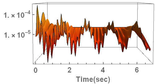
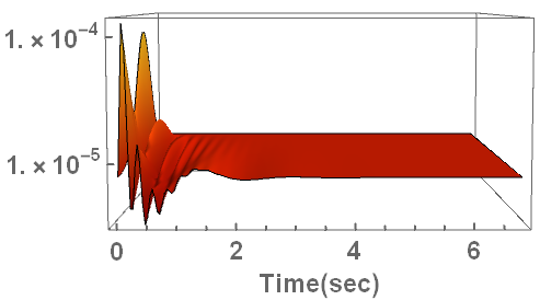
Figure 2: Rapid decay of the bending $w(x,t)$ in a few seconds (real time) after the controller applies.

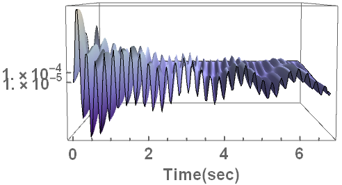
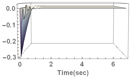
Figure 3: Rapid decay of the shear $\phi^{2}(x,t)$ in a few seconds (real time) after the controller applies.

The simulations in Figures 2 and 3 show that the $\phi^{2}$ and $w$ solutions both decay to zero fast enough. In fact, $\phi^{2}$ solution destabilizes in the beginning (the picking phenomenon in Fig. 4) but then it decays to zero faster than the bending solution. These results can be tuned up by using an improved scheme after a careful stability analysis is performed.

Note the necessity of the controller $P_{\varsigma}\dot{w}_{x}(L)$ in (41) to prove the strong stability result in Theorem 5. It is an open problem to analytically prove the same result without $P_{\varsigma}\dot{w}_{x}(L).$ In fact, further numerical investigation is the subject of Ozer-c (2018) where the impact of the non-classical feedback controller $V_{1}(t)=-k_{2}(P_{\varsigma}\dot{w}_{x})(L)$ over the classical one $V_{2}(t)=-k_{1}\dot{w}_{x}(L)$ is shown to be crucial (different feedback gains for each).

Models incorporating the nonlinear elasticity theory are also derived by a consistent variational approach, and the filtering technique is applied in Ozer-b (2018). The reader should refer to promising numerical results in Ozer-b (2018) with the choice of various nonlinear stabilizing feedback controllers. The results of this paper will be a basis for functional and numerical analyses for the nonlinear beam models in Ozer and Khenner (2018). Developing stable Finite Difference schemes and the adoption of the mixed-Finite Element method for both linear and nonlinear models are the progressing works Ozer-c (2018).

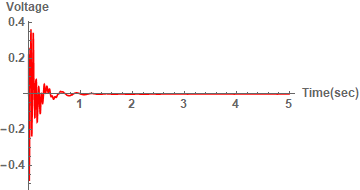
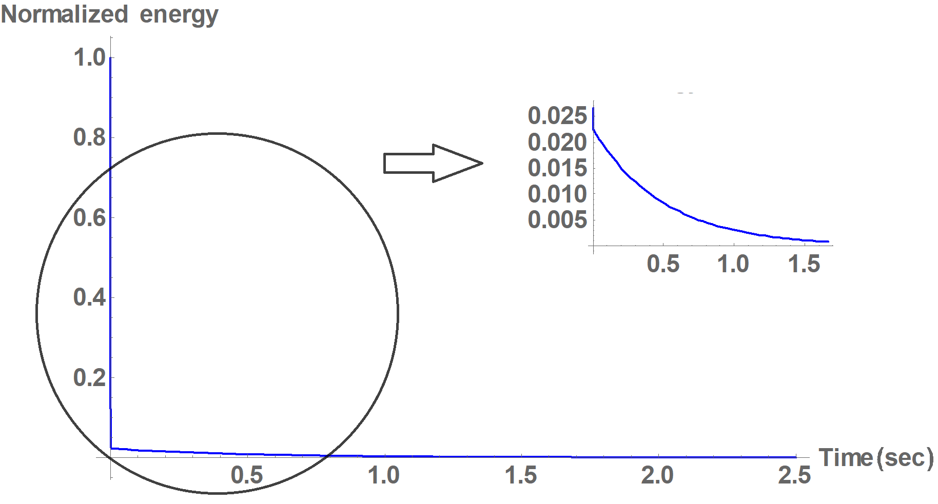
Figure 4: Voltage $V(t)$ and normalized energy $E(t)$ distributions for the first few seconds.

References

Allen and Hansen (2010) A.A. Allen, S. W. Hansen (2010). Analyticity and optimal damping for a multilayer Mead-Markus sandwich beam. Discrete Contin. Dyn. Syst. Ser. B, vol. 4-14, 1279-1292.
Banks et al (1991) H. T. Banks, K. Ito, and C. Wang (1991). Exponentially stable approximations of weakly damped
wave equations, Estimation and control of distributed parameter systems (Vorau, 1990), 1-33,Internat. Ser. Numer. Math., 100, Basel.
Baz (1997) A. Baz (1997). Boundary Control of Beams Using Active Constrained Layer Damping, J. Vib. Acoust, vol. 119-2, 166–172.
Bugariu et al. (2016) I. F. Bugariu, S. Micu, and I. Roventa, Approximation of the controls for the beam equation with vanishing viscosity, Mathematics of Computation 85-11, 2259–2303 (2016).
Hansen and Ozer (2010)S.W. Hansen, A.Ö. Özer (2010).
Exact boundary controllability of an abstract Mead-Marcus Sandwich beam model,
the Proc. of 53rd IEEE Conf. on Decision & Control, Atlanta, USA, 2578-2583.
Lam et al. (1997) M. J. Lam, D. Inman, W. R. Saunders (1997). Vibration Control through Passive Constrained Layer Damping and Active Control, Journal of Intelligent Material Systems and Structures, vol. 8-8, 663-677.
Leon and Zuazua (2002) L. Leon, E. Zuazua (2002). Boundary controllability of the finite-difference space semi-discretizations of the
beam equation, ESAIM Control Optim. Calc. Var. vol. 8, 827-862.
Liu and Liu (2002) K. Liu, Z.Liu (2002) Boundary stabilization of a nonhomogenous beam by the frequency domain multiplier method, Computation and Applied Mathematics, vol. 21-1, 299-313.
Morris and Ozer (2014) K.A. Morris, A.Ö. Özer (2014). Modeling and stabilizability of voltage-actuated piezoelectric beams with magnetic effects, SIAM J. Cont. Optim., vol. 52–4, 2371–2398.
Ozer (2015) A.Ö. Özer (2015).
Further stabilization and exact observability results for voltage-actuated piezoelectric beams with magnetic effects, Mathematics of Control, Signals, and Systems, vol. 27-2, 219–244.
Ozer (2016) A.Ö. Özer (2016). Semigroup well-posedness of a voltage controlled active constrained layered (ACL) beam with magnetic effects. Proc. of the American Control Conference, Boston, USA, 4580-4585.
Ozer-a (2017) A.Ö. Özer (2017). Modeling and Controlling an Active Constrained Layer (ACL) Beam Actuated by Two Voltage sources with/without Magnetic Effects, IEEE Trans. of Automatic Control, vol. 62-12, 6445-6450.
Ozer-b (2017) A.Ö. Özer (2017). Dynamic and electrostatic modeling for a piezoelectric smart composite and related stabilization results, submitted.
Ozer-a (2018) A.Ö. Özer (2017). Potential formulation for charge or current-controlled piezoelectric smart composites and stabilization results: electrostatic vs. quasi-static vs. fully-dynamic approaches, submitted.
Ozer-b (2018) A.Ö. Özer (2018). Nonlinear modeling and preliminary stabilization results for a class of piezoelectric smart composite beams, accepted, Proc. SPIE Active and Passive Smart Struc. and Integrated Systems.
Ozer-c (2018) A.Ö. Özer (2018). Stabilization and approximation results for a class of nonlinear smart composite beams, in prep.
Ozer and Hansen (2013) A.Ö. Özer, S.W. Hansen (2013).
Uniform stabilization of a multi-layer Rao-Nakra sandwich beam, Evolution Equations and Control Theory, vol. 2-4, 195–210.
Ozer and Hansen (2014) A.Ö. Özer, S.W. Hansen (2014).
Exact boundary controllability results for a multilayer Rao-Nakra sandwich beam, SIAM J. Cont. Optim., vol. 52-2, 1314–1337.
Ozer and Khenner (2018) A.Ö. Özer, M. Khenner, Numerical investigation of boundary controlled nonlinear piezoelectric beams, in prep.
Smith (2005) R.C. Smith (2005), Smart Material Systems, Society for
Industrial and Applied Mathematics.
Tebou and Zuazua (2007) L.T. Tebou, E. Zuazua (2007). Uniform boundary stabilization of the finite difference space discretization of
the 1-d wave equation.Adv. Comput. Math., vol. 26, 337-365.
Trindade and Benjendou (2002) M. Trindade and A. Benjendou (2002). Hybrid Active-Passive Damping Treatments Using Viscoelastic and Piezoelectric Materials:Review and Assessment, Journal of Vibration and Control, vol. 8, 699–745.
Yang and Wang (2017) C. Yang, J.M. Wang (2017). Exponential stability of an active constrained layer beam actuated by a voltage source without magnetic effects. Journal of Mathematical Analysis and Applications, vol. 448–2, 1204–1227.
Wang et al. (2006) J. M. Wang, B. Z. Guo and B. Chentouf (2006). Boundary feedback stabilization of a three-layer sandwich beam: Riesz basis approach, ESAIM Control Optim. Calc. Var., vol. 12, 12–34.
Wang and Guo (2008) J.M. Wang, B.Z. Guo (2008). Analyticity and Dynamic Behavior of a Damped
Three-Layer Sandwich Beam. J. Optim. Theory Appl., vol. 137, 675–689.