Janus Collaboration
Aging rate of spin glasses from simulations matches experiments
Abstract
Experiments on spin glasses can now make precise measurements of the exponent governing the growth of glassy domains, while our computational capabilities allow us to make quantitative predictions for experimental scales. However, experimental and numerical values for have differed. We use new simulations on the Janus II computer to resolve this discrepancy, finding a time-dependent , which leads to the experimental value through mild extrapolations. Furthermore, theoretical insight is gained by studying a crossover between the and fixed points.
The study of spin glasses (SGs) Mydosh (1993); Young (1998) has long been a key problem in statistical mechanics, providing ideas that have born fruit in fields as diverse as econophysics, biology or optimization in computer science. From a fundamental point of view, SGs are paradigmatic as the most approachable model for glassy behavior, both experimentally and theoretically. However, despite this relative simplicity, SG experiments and theory have traditionally developed separately, for practical and conceptual reasons. On the one hand, numerical simulations were not long enough to reach experimental times, while experiments were not precise enough or even able to measure key physical quantities. On the other hand, experimental samples are perennially out of equilibrium, while theory mostly focuses on the (unreachable) equilibrium phase.
In a typical experiment, the system is rapidly cooled to a subcritical working temperature and its off-equilibrium evolution (aging) studied. As the waiting time increases, the size of the glassy domains is seen to grow as , with an exponent that is expected to behave as Marinari et al. (2000). In traditional experiments Joh et al. (1999), based on the shift of the peak in the relaxation rate , was difficult to measure. Fortunately, the availability of excellent samples with a film geometry has suggested a new approach to the precision measurement of Zhai et al. (2017). The time that needs to saturate to the film thickness relates to the activation energies Guchhait and Orbach (2014, 2017). Varying the film thickness from 9 to 20 nm resulted in the measurement Zhai et al. (2017), very far from the value predicted by numerical simulations Belletti et al. (2008), Lulli et al. (2016).
Fortunately, recent theoretical progress makes it feasible to address the above-mentioned disagreement. A key development has been the introduction of the Janus Belletti et al. (2009a); Baity-Jesi et al. (2012) and Janus II Baity-Jesi et al. (2014a) computers, which have extended the numerical exploration of the dynamics almost to the experimental scale Belletti et al. (2008); Baity-Jesi et al. (2017a). In addition, the introduction of quantitative statics-dynamics dictionaries (first based on microscopic quantities Belletti et al. (2008); Alvarez Baños et al. (2010a, b) and more recently on experimentally measurable features Baity-Jesi et al. (2017a)) has clarified the relevance of the equilibrium phase for the off-equilibrium dynamics and showed how to extrapolate simulations to the experimental scale. Finally, the (macroscopic) experimental measurement of the size of glassy domains was shown to be consistent with the (microscopic) definition based on correlation functions Baity-Jesi et al. (2017b).
Here we resolve the discrepancy in by finding a (very mild) scale dependence in the dynamical exponent . We first recognize that time should be traded by length scales. Gentle extrapolations to the relevant experimental scales of 20 nm Zhai et al. (2017) then reconcile the numerical and experimental measurements. Such a computation has been possible only thanks to new data with unprecedented precision, achieved by reducing the uncertainty due to thermal fluctuations, an issue that was typically neglected in previous numerical work. From the theoretical point of view, our study is based on a characterization of the crossover between critical and low-temperature behavior. This is a very important point, since it resolves a theoretical controversy on how low a temperature must be studied to be free of critical effects, with some authors choosing to work at very low at the expense of the system sizes that it is possible to equilibrate (e.g., Wang et al. (2017)) and others trying to find a tradeoff between temperature and system size (e.g., Alvarez Baños et al. (2010a)).
We consider the standard Edwards-Anderson model Edwards and Anderson (1975), defined on a three-dimensional cubic lattice of side , on whose nodes we place spins that interact with their lattice nearest neighbors through
| (1) |
For each disorder realization (a sample), each of the quenched couplings is with probability. We shall refer to thin CuMn films Zhai et al. (2017), where the film thickness of 20 nm translates to a distance of 38 lattice spacings (the typical Mn-Mn distance is Å).
Our systems are initialized with random orientations for the spins (representing a very high starting temperature) and immediately quenched to the working temperature Baity-Jesi et al. (2013). We then follow the evolution with the waiting time (measured in units of full lattice sweeps) at constant temperature. For each sample we simulate real replicas, evolving with different thermal noise. We estimate our statistical errors with a jackknife method Amit and Martín-Mayor (2005) (including fit parameters Yllanes (2011)).
Our basic observable is the spatial autocorrelation of the overlap field (discussed in detail in Belletti et al. (2009b)),
| (2) | ||||
| (3) |
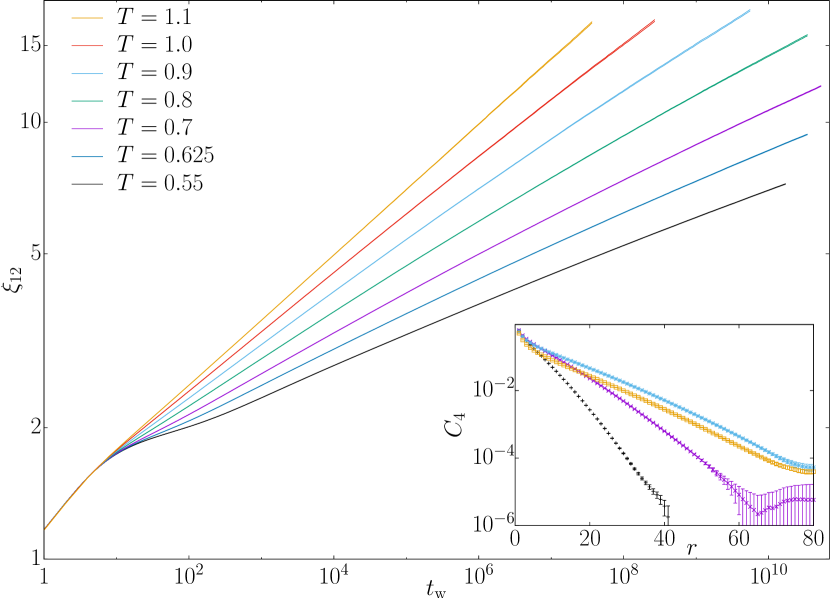
In these equations, the indices label the different real replicas; is the average over the thermal noise [in practice, an average over the pairs] and is the average over the disorder. In equilibrium simulations, by far the main source of error are the sample-to-sample fluctuations. Therefore, it has been customary to simulate the smallest that permits definitions such as (2) and maximize the number of samples. Instead, we have and . This choice, motivated to facilitate future studies of temperature chaos Janus Collaboration , has proven crucial: contrary to our expectations, the increase in has produced a dramatic reduction of statistical errors (see Appendix A for details). As a result, we have been able to follow the decay of over six decades (see inset to Fig. 1). A similar dramatic error reduction with high has also been seen in studies of the Gardner transition in structural glasses Berthier et al. (2016); Seoane and Zamponi (ress).
These correlation functions decay with distance as
| (4) |
so the growing can be computed through integral estimators Belletti et al. (2008, 2009b): . Then . As in recent work Belletti et al. (2009b); Baity-Jesi et al. (2017b, a); Fernández and Martín-Mayor (2015) we use (see Fernández et al. (2018) for technical details). The resulting is plotted in Fig. 1 for all our working temperatures.
The numerical Belletti et al. (2008, 2009b); Fernández and Martín-Mayor (2015) and experimental Zhai et al. (2017) state of the art describes the growth of with a power law,
| (5) |
However, with our increased precision, (5) is no longer a faithful representation of the dynamics. Indeed, if we switch to as independent variable we can interpolate our data as
| (6) |
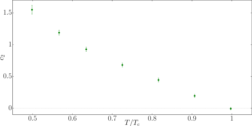
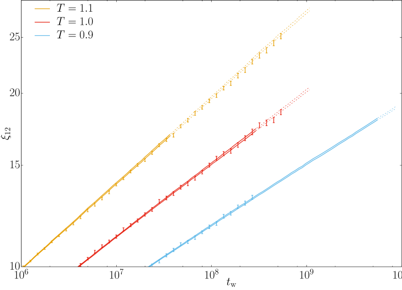
Notice that would reduce to (5), while would indicate a slowing down of the dynamics for increasing . Indeed, see Fig. 2, we find that vanishes only at , with 111 Our result is significantly more accurate that Lulli et al. (2016) and Belletti et al. (2008), even though, unlike Ref. Belletti et al. (2008), we allow for corrections to scaling, which increases the statistical error, see Appendix D. Of course, (6), useful as an interpolation, is not suitable to extrapolate for longer times than simulated. In order to do that, we need some insight from theory 222A naive explanation for the curvature in would be the existence of finite-size effects (see Belletti et al. (2008)). However, grows as we decrease , while finite-size effects would be controlled by , which is smaller for the lower temperatures. See Appendix B for extensive checks that our are safe..
We can gain much insight into the SG phase by considering the algebraic prefactor in (4), determined by an exponent . At , , where Baity-Jesi et al. (2013) is the anomalous dimension. In the SG phase, there are differing expectations for in the two main theoretical pictures. The droplet description McMillan (1983); Bray and Moore (1978); Fisher and Huse (1986) expects coarsening domains and therefore . On the other hand, the replica symmetry breaking (RSB) theory expects space-filling domains where vanishes at constant as grows. In particular, is given by the replicon, a critical mode analogous to magnons in Heisenberg ferromagnets (see Alvarez Baños et al. (2010b) for a detailed discussion). The best previous numerical study of Belletti et al. (2009b), found , with a small dependence that was vaguely attributed to the effect of the critical point.
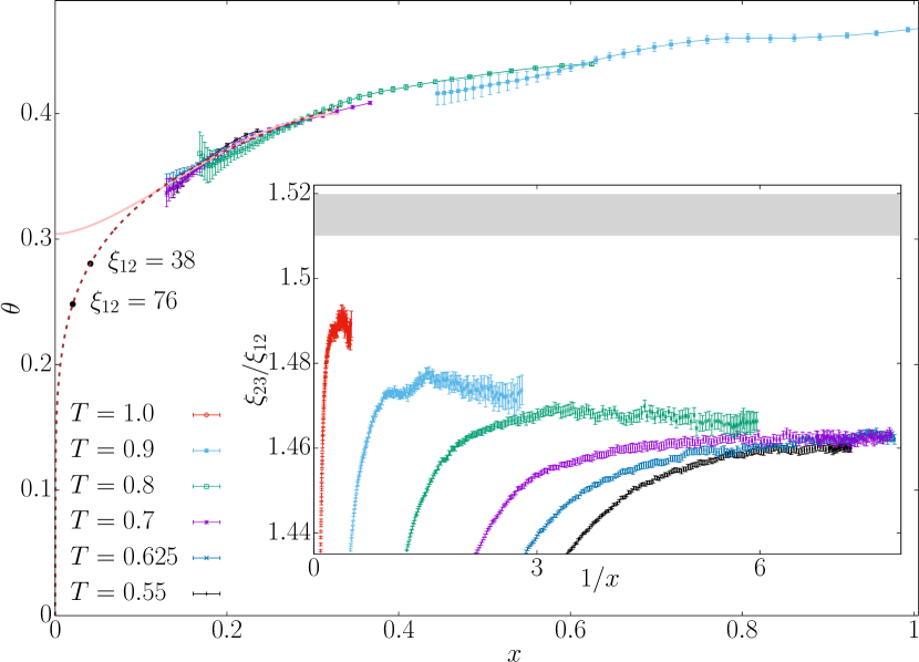
We can obtain by noticing that . However, again we find that, while is compatible with , for we actually have , slowly decreasing as increases (or decreases). This may seem an unsatisfactory result, since, in the large- limit, should tend to a -independent constant (possibly zero). The simplest explanation is that low values of are affected by the fixed point with [an idea supported by the higher measured for the higher ], while for we should see a crossover to the fixed point, with an unknown (see also Fernández and Martín-Mayor (2015)).
In analogy with the ferromagnetic phase of the model, we can model this crossover in terms of a Josephson length Josephson (1966). Close to , this should grow as , with Baity-Jesi et al. (2013), while scaling corrections are expected for the lowest temperatures 333In theory, , where we include analytic () and confluent ( scaling corrections with Baity-Jesi et al. (2013). For Fig. 3, we have chosen and to obtain the best collapse for the lowest temperatures.. If this hypothesis is correct, our data for different temperatures should come together when plotted in terms of a scaling variable . We test this scaling in the inset to Fig. 3, where we consider the ratio between two different determinations of the coherence length, which should be scale invariant in the large- limit (different definitions of all grow at the same rate, but differ in a small constant factor, see Fig. 4 in Belletti et al. (2009b)). As expected, there is an enveloping curve for the data at different . In particular, the curves for appear free from the influence of the critical point.
Similarly,, which we can compute numerically (see Appendix C), turns out to be a function of , see the collapsing curve Fig. 3. We are interested in estimating at the experimentally relevant scale of for thin films, recall our discussion of (1). As discussed, the RSB and droplet pictures have diverging expectations for , that is, for the limit, so we can use them as upper and lower bounds. In the RSB theory, see Appendix C and Fig. 3, we can compute an extrapolation to , although we take as our upper bound for . In the droplet description, we expect , where is in principle the stiffness exponent Boettcher (2004). As in Alvarez Baños et al. (2010a), we find that the droplet behavior can be reached in the infinite- limit, but only with a smaller exponent , which, furthermore, is highly sensitive to the fitting range. Using the droplet extrapolation for we obtain . Since our microscopically determined may differ by a small constant factor from a macroscopic measurement of Baity-Jesi et al. (2017b) we have also considered , which brings the exponent down to (see Fig. 3). In short, as observed in previous work Alvarez Baños et al. (2010a, b), for the experimentally relevant scale the physics is well described by a non-coarsening picture, with depending on the theory we use to extrapolate the data and the exact value chosen for the experimental scale.
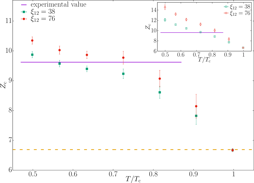
As discussed in the introduction, experiments observe a constant Zhai et al. (2017). In the previous discussion, on the other hand, we have found and a growing . Therefore, in order to compare our results with experiments, the first step is finding some way to extrapolate for . The most natural possibility, given the smoothness of the data in Fig. 1, is to assume that , with a that tends to a finite when , , thus
| (7) |
where is the exponent that controls finite- corrections. At , we expect Baity-Jesi et al. (2013); Lulli et al. (2016); Fernández and Martín-Mayor (2015). For , the leading behavior is given by (Alvarez Baños et al. (2010b) and section 4.2 in Alvarez Baños et al. (2010a)). When fitting to (7), in principle one must consider possible systematic effects from the fitting range and the increased statistical error due to our uncertainty in the value of . However, see Appendix D, these effects have little impact on our final estimates.
An alternative interpretation is to consider a crossover to activated dynamics, as proposed by the Saclay group Bouchaud et al. (2001); Berthier and Bouchaud (2002). Free-energy barriers are considered from a dynamical point of view, with a growth exponent ,
| (8) |
hence . Eq. (8) is a refinement of droplet theory Fisher and Huse (1986) and has been used before in experiments Schins et al. (1993) and simulations Rieger (1993) with values of 444 in (8) goes to zero at as , which is another form of the Josephson scaling.. RSB theory is neutral with respect to choosing ansatze (7) or (8). We recall the numerical result in infinite dimensions Billoire and Marinari (2001) of for the time scales associated with the largest energy barriers, with (see also Rogers and Moore (1989); Colborne (1990)). This result can be connected with finite at the upper critical dimensions , which yields . We note, in particular, that (7) can be regarded as a limit of (8). With previous data it was not possible to distinguish the behavior of (8) and that of a simple power law Belletti et al. (2009b). With the present simulations, we find that (8) also yields good fits for , with (again, the dependence on the fitting range is minimal, see Appendix D).
Therefore, both (7) and (8) can explain the behavior of the data for the simulated scales. In order to see whether they are useful to explain the experiments we consider the quantity , where is the derivative of either (7) or (8) at . The result is plotted in Fig. 4 (see Appendix D for the full fit parameters). Remarkably, the convergent ansatz of (7) produces an almost constant in a wide range, which additionally fits well the experimental value of . The activated dynamics of (8), on the other hand, is not a good fit for the experimental behavior (inset to Fig. 4).
Using simulations for very large systems with many replicas on Janus II we have found that the growth of the SG coherence length is controlled by a time-dependent exponent. After describing the dynamics as governed by a crossover between a critical and a low-temperature fixed point, we have been able to model this growth quantitatively and to extrapolate to experimental length scales. The resulting exponent is consistent with the most recent experimental measurements for power-law dynamics. In addition, we find clear evidence of non-coarsening dynamics at the experimental scale and find that temperatures are free of critical effects and therefore safe for numerical studies of the SG phase.
An open question concerns the generality of these results. Indeed, CuMn is a Heisenberg, rather than Ising, SG. However, even the purest Heisenberg system has unavoidable anisotropies, such as Dzyaloshinsky-Moriya interactions Bray and Moore (1982). These interactions, though tiny, extend over dozens of lattice spacings, which magnifies their effect. In fact, we know that Ising is the ruling universality class in the presence of coupling anisotropies Baity-Jesi et al. (2014b). We also remark that high-quality measurements on GeMn are excellently fit with Ising scaling laws Guchhait and Orbach (2017). Our results also match the most recent and accurate measurements on CuMn Zhai et al. (2017).
More generally, this study is a clear demonstration of the importance of high-precision results for the investigation of glassiness. Indeed, reducing the errors has shown that the aging rate slows down during the dynamics, contrary to previous findings. A similar change of paradigm might happen for structural glasses.
Acknowledgements.
We thank R. Orbach for encouraging discussions. This work was partially supported by Ministerio de Economía, Industria y Competitividad (MINECO) (Spain) through Grants No. FIS2013-42840-P, No. FIS2015-65078-C2, No. FIS2016-76359-P, and No. TEC2016-78358-R, by the Junta de Extremadura (Spain) through Grant No. GRU10158 (partially funded by FEDER) and by the DGA-FSE (Diputación General de Aragón – Fondo Social Europeo). This project has received funding from the European Research Council (ERC) under the European Union’s Horizon 2020 research and innovation program (Grant Nos. 694925 and 723955 - GlassUniversality). D. Y. acknowledges support by the Soft and Living Matter Program at Syracuse University.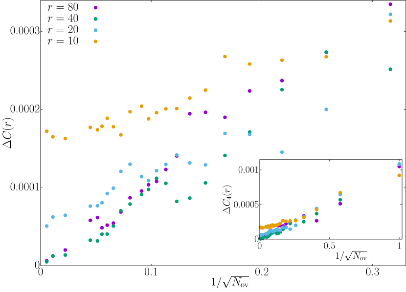
Appendix A Error reduction for high number of replicas
As mentioned in the main paper, the choice of the number of replicas () and samples () was taken with the aim of improving the estimation of observables related to temperature chaos in future work, where it is important to maximize the number of possible overlaps (pairs of replicas) .
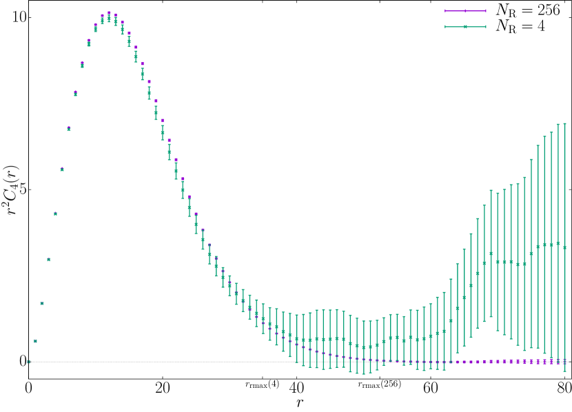
Unexpectedly, this has led to a dramatic increase in precision. Fig. 5 shows the reduction of the statistical error in the correlation function as a function of . Moreover, this effect is enhanced as increases, which leads to a qualitative improvement in the computation of the integrals (Fig. 6).
Appendix B Controlling finite-size effects
In order to obtain an estimate for we need to compute the integrals
| (9) |
As discussed in Belletti et al. (2009b), the main difficulty in this computation is handling the large- tail where relative errors [] are big. We have to consider two issues: a) how to minimize the statistical errors and b) how to check for finite-size effects (which will appear when becomes relatively large).
As explained in more detail in Belletti et al. (2009b); Fernández et al. (2018), our estimate of is the sum of the numerical integral of our measured up to a self-consistent cutoff and a tail contribution estimated with a smooth extrapolating function .
In short, the procedure is
-
1.
Obtain with fits of in a self-consistent region where the signal-to-noise ratio is still good.
-
2.
Integrate numerically up to some cutoff and add the analytical integral of beyond the cutoff to estimate the tail contribution.
There are several choices as to how to implement these steps, which we have used to control for systematic effects. For the extrapolating function , we consider first
| (10) |
Where is the replicon exponent discussed in the text and we fit for and . This analytical form is motivated by the fact that this is the simplest choice that avoids a pole singularity in the Fourier transform of at finite . In order to check for finite-size effects we also consider a second function resulting from fits that include the first-image term:
| (11) |
so we have a second extrapolating function
| (12) |
For these fits we used . However, this value has very little effect on the final computation of . We have checked this by recomputing the integrals with and (prediction of the droplet theory and influence of the fixed point respectively). The different choices of led to a systematic effect smaller than of the error bars in the worst case.
Once we have our two extrapolating functions and we can combine them with the data in several ways:
| (13) | |||||
| (14) | |||||
| (15) |
The difference between and is always under in the error, so choosing between them has no effect in any computation. In contrast, and present measurable differences for long , at least for our highest temperatures, where the faster dynamics allows us to reach higher values of . As a (very conservative) cutoff we have discarded all the where is larger than of the error bar, thus obtaining a below which we are assured not to have any finite-size effects in our systems. The reader can find the values in table 1.
| - | - | - | - |
As a final check that our data is not affected by finite-size effects, we have compared our with that of Fernández and Martín-Mayor (2015). This reference considers shorter simulations but with and samples. As shown in Fig. 7, the and data coincide even beyond our cutoff .
Appendix C Josephson Crossover
In this section we will give additional details on the Josephson crossover which describes how changes from being dominated by the fixed point to being dominated by the behavior as and vary. Assuming that , the crossover takes the form:
| (16) |
In this equation, is an analytical function decaying as . The prefactor for is fixed by the condition that the two asymptotic expansions connect smoothly at . We arrive at an asymptotic expansion for the integrals:
| (17) |
where and are amplitudes. Finally, we need to eliminate the unknown in favor of the computable ,
| (18) |
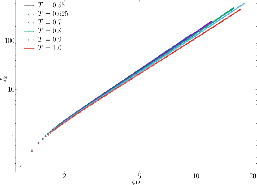
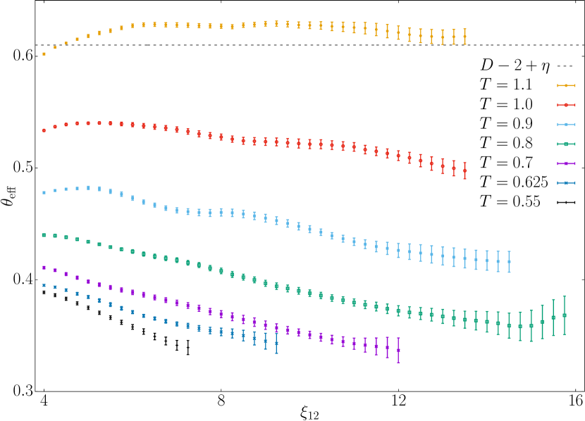
where considers contributions both from the numerator () and from the denominator. The easiest way to obtain is to study the evolution of as a function of . However, we have to settle for using as independent variable (see Fig. 8).
We can define an effective as
| (19) | ||||
| (20) |
To estimate this derivative for a given , we fit to a quadratic polynomial in in a window. We then take the derivative of this polynomial at . The procedure, as well as the wiggles in the resulting values of due to the extreme data correlation (see Fig. 9) may remind the reader of Fig. 1 in Belletti et al. (2008).
We have computed a fit to the first two terms in (20) in the range , resulting in the value of reported in the main text.
The previous analysis solves the problem of the crossover between the and fixed points. However, in the framework of the droplet picture one would also need to consider corrections to scaling at the fixed point. This is precisely what the droplet fit in the main text to does.
Appendix D Parameter choices in our fits
We will discuss separately the choice of for different temperatures and the choice of the value of .
D.1 Selection of for each temperature
We have reported fits of our data to three different functional forms
| (21) | ||||
| (22) | ||||
| (23) |
In these fits we have used and (), (), as discussed in the main text. Full results for the fits to (22) and (23) can be seen in tables 3 and 4, for different fitting ranges. We include for both cases the extrapolated values of for the experimental scale (as explained in the main text we use both and ) and for (22) also the value of the aging rate .
In order to make the choice of fitting range for the values plotted in the paper we have followed two criteria. Firstly we require the parameters of the fit to be stable inside the error when we increase . Secondly, we impose that be monotonically increasing in (with the exception of , which has different behavior). Table 2 shows our final choices for , which is the same for all three fits.
D.2 Selection of
For our most important result, namely the extrapolation of the aging rate to the experimental scale of , we have repeated our fits with our upper and lower bounds for (RSB and droplet extrapolations, respectively). The results are completely compatible, as we can see in table 5.
| = 3.5 | = 4 | = 5 | = 6 | = 7 | = 8 | = 9 | ||
|---|---|---|---|---|---|---|---|---|
| 23.61(28) | 24.22(40) | 25.30(86) | 22.9(31) | |||||
| 19.49(15) | 19.80(20) | 20.32(41) | 19.2(14) | |||||
| 20.38(18) | 20.75(24) | 21.39(51) | 20.0(18) | |||||
| /dof | 10.2(54)/111 | 3.0(12)/73 | 1.71(76)/40 | |||||
| 19.85(17) | 20.26(23) | 20.60(41) | 20.16(84) | |||||
| 16.538(91) | 16.74(12) | 16.90(19) | 16.71(37) | |||||
| 17.25(11) | 17.50(14) | 17.69(24) | 17.45(47) | |||||
| /dof | 81(34)/167 | 18(10)/147 | 8.3(21)/114 | 5.1(19)/86 | ||||
| 17.04(18) | 17.23(21) | 17.61(27) | 18.23(35) | 18.63(62) | ||||
| 14.295(88) | 14.38(11) | 14.55(13) | 14.81(15) | 14.96(25) | ||||
| 14.89(11) | 15.00(13) | 15.21(16) | 15.54(19) | 15.75(32) | ||||
| /dof | 116(40)/190 | 66(36)/173 | 33(24)/144 | 9.3(84)/119 | 4.9(21)/98 | |||
| 13.76(15) | 14.06(19) | 14.53(26) | 15.19(35) | 15.68(42) | 16.18(58) | 16.55(78) | ||
| 11.787(73) | 11.921(89) | 12.11(12) | 12.37(15) | 12.55(17) | 12.73(22) | 12.85(28) | ||
| 12.211(93) | 12.38(11) | 12.63(15) | 12.98(19) | 13.23(23) | 13.47(30) | 13.65(39) | ||
| /dof | 351(104)/185 | 188(72)/170 | 93(41)/146 | 27(16)/125 | 12.4(82)/107 | 6.2(31)/91 | 4.9(21)/77 | |
| 11.00(13) | 11.29(18) | 11.54(24) | 11.80(31) | 12.55(41) | 13.16(68) | 12.3(13) | ||
| 9.748(65) | 9.883(93) | 9.98(11) | 10.08(13) | 10.34(16) | 10.55(25) | 10.33(41) | ||
| 10.017(82) | 10.18(11) | 10.32(14) | 10.45(17) | 10.82(21) | 11.11(34) | 10.80(60) | ||
| /dof | 310(150)/165 | 129(64)/152 | 79(44)/131 | 63(35)/113 | 22(13)/98 | 5.9(21)/84 | 6.4(79)/72 | |
| 8.60(11) | 8.69(15) | 8.83(20) | 8.97(53) | 9.29(45) | 9.36(46) | 10.28(89) | ||
| 8.041(59) | 8.080(73) | 8.132(93) | 8.21(22) | 8.27(18) | 8.34(17) | 8.63(32) | ||
| 8.162(74) | 8.210(86) | 8.28(11) | 8.38(29) | 8.46(24) | 8.57(24) | 8.98(44) | ||
| /dof | 43(30)/137 | 27(18)/126 | 16(13)/107 | 12(25)/91 | 10.4(91)/78 | 8.4(60)/66 | 2.9(21)/55 | |
| 6.672(44) | 6.671(41) | 6.689(63) | 6.751(84) | 6.80(12) | 7.00(18) | 7.02(21) | ||
| 6.682(32) | 6.673(41) | 6.694(50) | 6.732(68) | 6.77(10) | 6.92(14) | 6.94(16) | ||
| 6.677(33) | 6.671(41) | 6.691(54) | 6.742(72) | 6.79(11) | 6.96(16) | 6.99(16) | ||
| /dof | 32(19)/119 | 31(20)/109 | 26(16)/92 | 19(10)/78 | 16.8(74)/66 | 5.9(20)/55 | 6.3(27)/46 |
| = 3.5 | = 4 | = 5 | = 6 | = 7 | = 8 | = 9 | ||
|---|---|---|---|---|---|---|---|---|
| 24.07(41) | 24.25(55) | 24.6(11) | 24.7(81) | |||||
| 28.86(69) | 29.18(95) | 29.9(19) | 30(15) | |||||
| 13.78(65) | 13.45(92) | 12.8(18) | 18(13) | |||||
| 0.3512(92) | 0.355(21) | 0.372(33) | 0.29(24) | |||||
| /dof | 13.3(47)/133 | 6.8(20)/111 | 3.2(15)/73 | 1.7(27)/40 | ||||
| 19.73(22) | 19.72(28) | 19.36(45) | 18.53(77) | |||||
| 23.33(38) | 23.31(49) | 22.66(79) | 21.1(13) | |||||
| 10.36(37) | 10.39(52) | 11.3(11) | 14.0(30) | |||||
| 0.354(14) | 0.352(12) | 0.334(21) | 0.290(39) | |||||
| /dof | 19(10)/167 | 15(10)/147 | 8.5(33)/114 | 4.5(14)/86 | ||||
| 16.58(22) | 16.44(23) | 16.35(27) | 16.51(32) | 16.55(52) | ||||
| 19.40(37) | 19.14(40) | 18.98(47) | 19.29(58) | 19.4(10) | ||||
| 7.32(34) | 7.63(43) | 7.84(59) | 7.41(75) | 7.3(14) | ||||
| 0.364(13) | 0.354(12) | 0.354(24) | 0.358(23) | 0.360(39) | ||||
| /dof | 49(38)/190 | 28(20)/173 | 10.5(83)/144 | 6.3(31)/119 | 5.7(29)/98 | |||
| 13.37(18) | 13.39(21) | 13.45(25) | 13.68(31) | 13.80(35) | 13.94(45) | 14.1(17) | ||
| 15.44(33) | 15.48(37) | 15.60(46) | 16.06(59) | 16.31(68) | 16.59(93) | 17.1(38) | ||
| 4.16(25) | 4.13(29) | 4.01(38) | 3.57(43) | 3.36(48) | 3.13(66) | 3.0(19) | ||
| 0.392(13) | 0.390(19) | 0.395(18) | 0.421(27) | 0.443(31) | 0.447(50) | 0.46(18) | ||
| /dof | 31(19)/185 | 29(19)/170 | 22(17)/146 | 10.0(60)/125 | 7.5(34)/107 | 5.5(21)/91 | 5(11)/77 | |
| 10.76(17) | 10.86(21) | 10.82(24) | 10.86(27) | 11.23(35) | 11.49(54) | 11.13(56) | ||
| 12.12(30) | 12.31(39) | 12.24(45) | 12.31(53) | 13.12(73) | 13.7(12) | 12.9(12) | ||
| 2.15(19) | 2.01(23) | 2.07(31) | 2.00(39) | 1.52(31) | 1.18(45) | 1.67(77) | ||
| 0.417(23) | 0.430(34) | 0.431(28) | 0.427(41) | 0.490(51) | 0.546(88) | 0.47(10) | ||
| /dof | 68(44)/165 | 46(25)/152 | 41(25)/131 | 38(24)/113 | 17(10)/98 | 8.7(45)/84 | 4.8(25)/72 | |
| 8.53(15) | 8.54(18) | 8.55(20) | 8.56(30) | 8.59(60) | 8.74(72) | 9.22(18) | ||
| 9.19(27) | 9.20(33) | 9.22(39) | 9.25(58) | 9.3(12) | 9.7(16) | 10.9(45) | ||
| 0.85(14) | 0.84(18) | 0.83(22) | 0.79(40) | 0.7(10) | 0.5(10) | 1.4(19) | ||
| 0.440(36) | 0.441(51) | 0.444(64) | 0.45(10) | 0.49(25) | 0.55(30) | 0.34(71) | ||
| /dof | 12.6(95)/137 | 12.1(90)/126 | 10.0(87)/107 | 9.3(83)/91 | 8.2(97)/78 | 07(11)/66 | 11(11)/55 | |
| 6.684(12) | 6.682(14) | 6.684(11) | 6.672(31) | 6.683(32) | 6.694(31) | 6.712(41) | ||
| 6.684(13) | 6.681(11) | 6.682(14) | 6.674(41) | 6.684(41) | 6.692(31) | 6.721(42) | ||
| 1.9(10) | 1.71(91) | 0.4(27) | 0.02(64) | 0.0(26) | 1.5(26) | 1.2(10) | ||
| -0.0030(49) | 0.0037(68) | 0.03(15) | 0.29(42) | 0.37(55) | 0.002(16) | 0.023(51) | ||
| /dof | 34(20)/119 | 33(19)/109 | 27(18)/92 | 25(18)/78 | 23(15)/66 | 21(14)/55 | 11.0(26)/46 |
| 19.80(20) | 20.08(22) | 20.75(24) | 21.41(27) | ||
| 16.90(19) | 17.07(20) | 17.69(24) | 18.13(27) | ||
| 14.81(15) | 14.93(16) | 15.54(19) | 15.87(21) | ||
| 12.73(22) | 12.81(23) | 13.47(30) | 13.71(32) | ||
| 10.55(25) | 10.61(26) | 11.11(34) | 11.28(37) | ||
| 8.63(32) | 8.68(33) | 8.98(44) | 9.02(42) | ||
References
- Mydosh (1993) J. A. Mydosh, Spin Glasses: an Experimental Introduction (Taylor and Francis, London, 1993).
- Young (1998) A. P. Young, Spin Glasses and Random Fields (World Scientific, Singapore, 1998).
- Marinari et al. (2000) E. Marinari, G. Parisi, F. Ricci-Tersenghi, J. J. Ruiz-Lorenzo, and F. Zuliani, J. Stat. Phys. 98, 973 (2000), arXiv:cond-mat/9906076 .
- Joh et al. (1999) Y. G. Joh, R. Orbach, G. G. Wood, J. Hammann, and E. Vincent, Phys. Rev. Lett. 82, 438 (1999).
- Zhai et al. (2017) Q. Zhai, D. C. Harrison, D. Tennant, E. D. Dalhberg, G. G. Kenning, and R. L. Orbach, Phys. Rev. B 95, 054304 (2017).
- Guchhait and Orbach (2014) S. Guchhait and R. Orbach, Phys. Rev. Lett. 112, 126401 (2014).
- Guchhait and Orbach (2017) S. Guchhait and R. L. Orbach, Phys. Rev. Lett. 118, 157203 (2017).
- Belletti et al. (2008) F. Belletti, M. Cotallo, A. Cruz, L. A. Fernandez, A. Gordillo-Guerrero, M. Guidetti, A. Maiorano, F. Mantovani, E. Marinari, V. Martín-Mayor, A. M. Sudupe, D. Navarro, G. Parisi, S. Perez-Gaviro, J. J. Ruiz-Lorenzo, S. F. Schifano, D. Sciretti, A. Tarancon, R. Tripiccione, J. L. Velasco, and D. Yllanes (Janus Collaboration), Phys. Rev. Lett. 101, 157201 (2008), arXiv:0804.1471 .
- Lulli et al. (2016) M. Lulli, G. Parisi, and A. Pelissetto, Phys. Rev. E 93, 032126 (2016).
- Belletti et al. (2009a) F. Belletti, M. Guidetti, A. Maiorano, F. Mantovani, S. F. Schifano, R. Tripiccione, M. Cotallo, S. Perez-Gaviro, D. Sciretti, J. L. Velasco, A. Cruz, D. Navarro, A. Tarancon, L. A. Fernandez, V. Martín-Mayor, A. Muñoz-Sudupe, D. Yllanes, A. Gordillo-Guerrero, J. J. Ruiz-Lorenzo, E. Marinari, G. Parisi, M. Rossi, and G. Zanier (Janus Collaboration), Computing in Science and Engineering 11, 48 (2009a).
- Baity-Jesi et al. (2012) M. Baity-Jesi, R. A. Baños, A. Cruz, L. A. Fernandez, J. M. Gil-Narvion, A. Gordillo-Guerrero, M. Guidetti, D. Iniguez, A. Maiorano, F. Mantovani, E. Marinari, V. Martín-Mayor, J. Monforte-Garcia, A. Munoz Sudupe, D. Navarro, G. Parisi, M. Pivanti, S. Perez-Gaviro, F. Ricci-Tersenghi, J. J. Ruiz-Lorenzo, S. F. Schifano, B. Seoane, A. Tarancon, P. Tellez, R. Tripiccione, and D. Yllanes, Eur. Phys. J. Special Topics 210, 33 (2012), arXiv:1204.4134 .
- Baity-Jesi et al. (2014a) M. Baity-Jesi, R. A. Baños, A. Cruz, L. A. Fernandez, J. M. Gil-Narvion, A. Gordillo-Guerrero, D. Iniguez, A. Maiorano, F. Mantovani, E. Marinari, V. Martín-Mayor, J. Monforte-Garcia, A. Muñoz Sudupe, D. Navarro, G. Parisi, S. Perez-Gaviro, M. Pivanti, F. Ricci-Tersenghi, J. J. Ruiz-Lorenzo, S. F. Schifano, B. Seoane, A. Tarancon, R. Tripiccione, and D. Yllanes (Janus Collaboration), Comp. Phys. Comm 185, 550 (2014a), arXiv:1310.1032 .
- Baity-Jesi et al. (2017a) M. Baity-Jesi, E. Calore, A. Cruz, L. A. Fernandez, J. M. Gil-Narvión, A. Gordillo-Guerrero, D. Iñiguez, A. Maiorano, E. Marinari, V. Martin-Mayor, J. Monforte-Garcia, A. Muñoz Sudupe, D. Navarro, G. Parisi, S. Perez-Gaviro, F. Ricci-Tersenghi, J. J. Ruiz-Lorenzo, S. F. Schifano, B. Seoane, A. Tarancón, R. Tripiccione, and D. Yllanes, Proceedings of the National Academy of Sciences 114, 1838 (2017a).
- Alvarez Baños et al. (2010a) R. Alvarez Baños, A. Cruz, L. A. Fernandez, J. M. Gil-Narvion, A. Gordillo-Guerrero, M. Guidetti, A. Maiorano, F. Mantovani, E. Marinari, V. Martín-Mayor, J. Monforte-Garcia, A. Muñoz Sudupe, D. Navarro, G. Parisi, S. Perez-Gaviro, J. J. Ruiz-Lorenzo, S. F. Schifano, B. Seoane, A. Tarancon, R. Tripiccione, and D. Yllanes (Janus Collaboration), J. Stat. Mech. 2010, P06026 (2010a), arXiv:1003.2569 .
- Alvarez Baños et al. (2010b) R. Alvarez Baños, A. Cruz, L. A. Fernandez, J. M. Gil-Narvion, A. Gordillo-Guerrero, M. Guidetti, A. Maiorano, F. Mantovani, E. Marinari, V. Martín-Mayor, J. Monforte-Garcia, A. Muñoz Sudupe, D. Navarro, G. Parisi, S. Perez-Gaviro, J. J. Ruiz-Lorenzo, S. F. Schifano, B. Seoane, A. Tarancon, R. Tripiccione, and D. Yllanes (Janus Collaboration), Phys. Rev. Lett. 105, 177202 (2010b), arXiv:1003.2943 .
- Baity-Jesi et al. (2017b) M. Baity-Jesi, E. Calore, A. Cruz, L. A. Fernandez, J. M. Gil-Narvion, A. Gordillo-Guerrero, D. Iñiguez, A. Maiorano, E. Marinari, V. Martin-Mayor, J. Monforte-Garcia, A. Muñoz Sudupe, D. Navarro, G. Parisi, S. Perez-Gaviro, F. Ricci-Tersenghi, J. J. Ruiz-Lorenzo, S. F. Schifano, B. Seoane, A. Tarancon, R. Tripiccione, and D. Yllanes (Janus Collaboration), Phys. Rev. Lett. 118, 157202 (2017b).
- Wang et al. (2017) W. Wang, J. Machta, H. Munoz-Bauza, and H. G. Katzgraber, Phys. Rev. B 96, 184417 (2017).
- Edwards and Anderson (1975) S. F. Edwards and P. W. Anderson, Journal of Physics F: Metal Physics 5, 965 (1975).
- Baity-Jesi et al. (2013) M. Baity-Jesi, R. A. Baños, A. Cruz, L. A. Fernandez, J. M. Gil-Narvion, A. Gordillo-Guerrero, D. Iniguez, A. Maiorano, F. Mantovani, E. Marinari, V. Martín-Mayor, J. Monforte-Garcia, A. Muñoz Sudupe, D. Navarro, G. Parisi, S. Perez-Gaviro, M. Pivanti, F. Ricci-Tersenghi, J. J. Ruiz-Lorenzo, S. F. Schifano, B. Seoane, A. Tarancon, R. Tripiccione, and D. Yllanes (Janus Collaboration), Phys. Rev. B 88, 224416 (2013), arXiv:1310.2910 .
- Amit and Martín-Mayor (2005) D. J. Amit and V. Martín-Mayor, Field Theory, the Renormalization Group and Critical Phenomena, 3rd ed. (World Scientific, Singapore, 2005).
- Yllanes (2011) D. Yllanes, Rugged Free-Energy Landscapes in Disordered Spin Systems, Ph.D. thesis, Universidad Complutense de Madrid (2011), arXiv:1111.0266 .
- Belletti et al. (2009b) F. Belletti, A. Cruz, L. A. Fernandez, A. Gordillo-Guerrero, M. Guidetti, A. Maiorano, F. Mantovani, E. Marinari, V. Martín-Mayor, J. Monforte, A. Muñoz Sudupe, D. Navarro, G. Parisi, S. Perez-Gaviro, J. J. Ruiz-Lorenzo, S. F. Schifano, D. Sciretti, A. Tarancon, R. Tripiccione, and D. Yllanes (Janus Collaboration), J. Stat. Phys. 135, 1121 (2009b), arXiv:0811.2864 .
- (23) Janus Collaboration, (in preparation) .
- Berthier et al. (2016) L. Berthier, P. Charbonneau, Y. Jin, G. Parisi, B. Seoane, and F. Zamponi, Proc. Natl. Acad. Sci. USA 113, 8397 (2016).
- Seoane and Zamponi (ress) B. Seoane and F. Zamponi, Soft Matter (2018, in press), 10.1039/C8SM00859K.
- Fernández and Martín-Mayor (2015) L. A. Fernández and V. Martín-Mayor, Phys. Rev. B 91, 174202 (2015).
- Fernández et al. (2018) L. A. Fernández, E. Marinari, V. Martín-Mayor, G. Parisi, and J. Ruiz-Lorenzo, “An experiment-oriented analysis of 2d spin-glass dynamics: a twelve time-decades scaling study,” (2018), submitted, arXiv:1805.06738 .
- Note (1) Our result is significantly more accurate that Lulli et al. (2016) and Belletti et al. (2008), even though, unlike Ref. Belletti et al. (2008), we allow for corrections to scaling, which increases the statistical error, see Appendix D.
- Note (2) A naive explanation for the curvature in would be the existence of finite-size effects (see Belletti et al. (2008)). However, grows as we decrease , while finite-size effects would be controlled by , which is smaller for the lower temperatures. See Appendix B for extensive checks that our are safe.
- McMillan (1983) W. L. McMillan, Phys. Rev. B 28, 5216 (1983).
- Bray and Moore (1978) A. J. Bray and M. A. Moore, Phys. Rev. Lett. 41, 1068 (1978).
- Fisher and Huse (1986) D. S. Fisher and D. A. Huse, Phys. Rev. Lett. 56, 1601 (1986).
- Josephson (1966) B. D. Josephson, Phys. Lett. 21, 608 (1966).
- Note (3) In theory, , where we include analytic () and confluent ( scaling corrections with Baity-Jesi et al. (2013). For Fig. 3, we have chosen and to obtain the best collapse for the lowest temperatures.
- Boettcher (2004) S. Boettcher, Eur. Phys. J. B 38, 83 (2004), arXiv:cond-mat/0310698 .
- Bouchaud et al. (2001) J.-P. Bouchaud, V. Dupuis, J. Hammann, and E. Vincent, Phys. Rev. B 65, 024439 (2001).
- Berthier and Bouchaud (2002) L. Berthier and J.-P. Bouchaud, Phys. Rev. B 66, 054404 (2002).
- Schins et al. (1993) A. G. Schins, A. F. M. Arts, and H. W. de Wijn, Phys. Rev. Lett. 70, 2340 (1993).
- Rieger (1993) H. Rieger, J. Phys. A 26, L615 (1993).
- Note (4) in (8\@@italiccorr) goes to zero at as , which is another form of the Josephson scaling.
- Billoire and Marinari (2001) A. Billoire and E. Marinari, Journal of Physics A: Mathematical and General 34, L727 (2001).
- Rogers and Moore (1989) G. Rogers and M. A. Moore, J. Phys. A: Math. Gen. 22, 1085 (1989).
- Colborne (1990) S. G. W. Colborne, J. Phys. A: Math. Gen. 23, 4013 (1990).
- Bray and Moore (1982) A. J. Bray and M. A. Moore, J. Phys. C: Solid St. Phys. 15, 3897 (1982).
- Baity-Jesi et al. (2014b) M. Baity-Jesi, L. A. Fernandez, V. Martín-Mayor, and J. M. Sanz, Phys. Rev. 89, 014202 (2014b), arXiv:1309.1599 .