A novel method for lepton energy calibration at Hadron Collider Experiments

Abstract

This report is to provide a novel method for the lepton energy calibration at Hadron Collider Experiments. The method improves the classic lepton energy calibration procedure widely used at hadron collider experiments. The classic method parameterizes the potential bias in the lepton energy calibration, and determines the value of the parameter by the invariant mass of $Z/\gamma^{*}\rightarrow\ell^{+}\ell^{-}$ events. The precision of the calibration is dominated by the number of parameters or terms considered in the parameterization, for example, a polynomial extension. With one physics constraint of the reconstructed $Z$ boson mass, the classic procedure can use and determine one parameter.

The novel method improves the precision of lepton calibration by introducing more terms in the parameterization. To precisely determine the values of multiple parameters, the method first acquires more constraints by separating the $Z/\gamma^{*}\rightarrow\ell^{+}\ell^{-}$ samples according to the decay kinematics, and then reduces the correlation between multiple parameters. Since the new method is still using the reconstructed $Z$ boson masses as the only constraints, it is much faster and easier than detailed study of detector simulations.

I I. Introduction

I.1 I-A. Lepton energy calibration

Measurement and reconstruction of electron and muon energy at hadron collider experiments are essential in many physics analyses. For experiments like D0 and CDF from the Fermilab Tevatron, and ATLAS and CMS from the CERN Large Hadron Collider (LHC), the determination of electron and muon energy scale is required to have a high precision for a wide range of energy from a few GeV up to $\mathcal{O}(1000)$ GeV. After various calibrations, the corrected lepton energy scale is required to be consistent with its true value:

$$\mathcal{E}(E_{\text{obs}}) \rightarrow \mathcal{E}(E_{\text{corr}})=\mathcal{E}(E_{\text{true}})$$ (1)

where $E_{\text{obs}}$ and $E_{\text{corr}}$ are the observed lepton energy and calibrated lepton energy. $E_{\text{true}}$ is the corresponding true energy. $\mathcal{E}$ means average or mathematical expectation on an ensemble of events, representing the energy scale. To satisfy this requirement, a widely used method has been developed at hadron collider experiments, to determine and calibrate electron and muon energy scale using the $Z/\gamma^{*}\rightarrow\ell^{+}\ell^{-}$ (dilepton) events. In this method, the lepton energy scale is determined by observing the dilepton invariant mass instead of directly looking into the energy spectrum. The reconstructed dilepton mass can be expressed as:

$$M^{2}=2E_{1}E_{2}(1-\cos\theta_{12}),$$ (2)

where $E_{1}$ and $E_{2}$ are the energy of the two leptons, and $\theta_{12}$ is the spatial opening angle between them. The invariant mass observed in the dilepton events, which is determined by the line shape of the $Z$ boson invariant mass spectra, has a very sharp peak, thus sensitive to the lepton energy scale. A scaling factor $k$ is applied to the lepton energy as a correction:

$$E_{\text{corr}} = k\cdot E_{\text{obs}}.$$ (3)

According to Eq. 2, we have

$$M^{2}_{\text{corr}} = k^{2}M^{2}_{\text{obs}},$$ (4)

Therefore, the energy calibration in Eq. 1 is equivalent to a mass calibration:

$$\mathcal{E}(M_{\text{obs}})\rightarrow\mathcal{E}(M_{\text{corr}}) = \mathcal{E}(M_{\text{true}})$$ (5)

$$= k\cdot\mathcal{E}(M_{\text{obs}}),$$

which means the correction $k$ on lepton energy scale can be determined by requiring the best agreement between the corrected mass mean $\mathcal{E}(M_{\text{corr}})$, and the “true” value $\mathcal{E}(M_{\text{true}})$. Most physics measurements are unbiased as long as energy scales in data and Monte Carlo (MC) simulations are consistent. Thus $\mathcal{E}(M_{\text{obs}})$ and $\mathcal{E}(M_{\text{true}})$ are the mass means observed in MC and data. Sometimes, physics measurements requires not only a consistent energy scale, but also an absolute energy calibration. In this case, $\mathcal{E}(M_{\text{true}})$ indeed represents the “true” value which can be acquired from generator level information.

The energy scale is determined by observing dilepton mass instead of lepton energy because of two main reasons. First, the overall uncertainty on the energy scale determination is dominated by the uncertainty of observing the mean value. The uncertainty of observing mean value from any gaussian-type sample is expressed as:

$$\frac{\delta\text{mean}}{\text{mean}}=\frac{\Delta}{\text{mean}\cdot\sqrt{N}}$$ (6)

where $\Delta$ is the standard deviation of the sample, and $N$ is the total number of events in this sample. As we know, the width of the $Z$ boson mass spectra is only a few GeV (including physics width and resolution of detector), while the width of the lepton energy distribution can be very large at hadron colliders. Therefore, the statistical uncertainty on $k$ factor is much smaller from the mass mean observation.

Second, the main contribution of the observed lepton energy at hadron colliders comes from the $Z$ boson boost and the finite $p_{T}$ of the $Z$ recoiling against some hadronic system. rather than the $Z$ boson mass. The $Z$ boson boost is determined by the difference of energy between initial quarks and anti-quarks of $q\bar{q}\rightarrow Z/\gamma^{*}$ annihilation, where quarks come from hadrons. It means parton distribution functions (PDFs) used in MC generation has impact. QCD calculation of initial state radiation also affects the lepton energy in MC. As a result, large effects from PDFs and QCD calculation will be absorbed in the difference between $\mathcal{E}(E_{\text{obs}})$ and $\mathcal{E}(E_{\text{true}})$, and further propagate to the energy scale determination. By observing invariant mass instead, the calibration is independent of PDFs and QCD calculation. It not only reduces the systematic uncertainty, but also is a necessary condition of absolute energy calibration.

In general, this method does not depend upon knowledge on understanding the source of the bias in energy measurement, such as multiple hadron interactions (pileup effects), energy loss and imperfect reconstruction algorithm. All these effects are absorbed in the $k$ factor as a simple parameterization. It is the reason that calibration using observed dilepton events is always applied as the final step after all detector and simulation level calibrations at hadron collider experiments.

Since the data accumulates very fast at hadron colliders with high luminosity, the $Z/\gamma^{*}\rightarrow\ell^{+}\ell^{-}$ sample can be very large. According to Eq. 6, a precision of lepton energy calibration of $0.01\%$ should be easily achieved using 10 M dilepton events, corresponding to a data sample collected by the ATLAS or the CMS detector within one year at 13 TeV ATLAS-Z-xsection .

I.2 I-B. Limited precision

In spite of an expected high precision, the calibration procedure described in section I-A has a much larger uncertainty which will not be reduced as data accumulating. As discussed, the calibration using dilepton events is a parameterization of any potential bias in the lepton energy measurement. A perfect parameterization can be written in the form of a polynomial expansion:

$$E_{\text{truth}}=b+k\cdot E_{\text{obs}}+\gamma\cdot E^{2}_{\text{obs}}+\cdot\cdot\cdot,$$ (7)

Higher order terms in Eq. 7 can be very small with modern detector design and construction, but offset term $b$ could be very large due to noise from pileup effects, resulting in a linear relationship between observed energy and its true value:

$$E_{\text{truth}}=b+k\cdot E_{\text{obs}}.$$ (8)

However, the calibration in Eq. 3 is using a single scaling parameterization, here denoted as $k^{\prime}$

$$E_{\text{obs}}\rightarrow E_{\text{corr}} = k^{\prime}\cdot E_{\text{obs}},$$ (9)

and still requires $\mathcal{E}(M_{\text{true}})=\mathcal{E}(M_{\text{corr}})$. Thus we have:

$$k^{\prime}\cdot\mathcal{E}(E_{\text{obs}}) \approx b+k\cdot\mathcal{E}(E_{\text{obs}})$$

$$k^{\prime}-k \approx \frac{b}{\mathcal{E}(E_{\text{obs}})},$$ (10)

Note that when $k^{\prime}$ is determined by observing mass, and $b$ is not negligible, Eq. I.2 can only hold as an approximation, which will be discussed later in section II-C. An energy-dependent bias then appears as:

$$\frac{E_{\text{corr}}-E_{\text{truth}}}{E_{\text{obs}}} = \frac{k^{\prime}\cdot E_{\text{obs}}-k\cdot E_{\text{obs}}-b}{E_{\text{obs}}}$$ (11)

$$= (k^{\prime}-k)\cdot\left[1-\frac{\mathcal{E}(E_{\text{obs}})}{E_{\text{obs}}}\right]$$

$$= \frac{b}{\mathcal{E}(E_{\text{obs}})}\left[1-\frac{\mathcal{E}(E_{\text{obs}})}{E_{\text{obs}}}\right].$$

The dependence is determine by $b/\mathcal{E}(E_{\text{obs}})$. For the $pp\rightarrow Z/\gamma^{*}\rightarrow\ell^{+}\ell^{-}$ events at $\sqrt{s}=13$ TeV, $\mathcal{E}(E_{\text{obs}})\sim\mathcal{O}(100)$ GeV. Even if $b$ is as small as 1 GeV, the dependence is $1\%$. When $k^{\prime}$ is applied to leptons which have their energy much higher than $\mathcal{E}(E_{\text{obs}})$, the bias on the corrected energy is approaching $\mathcal{O}(1\%)$. When $k^{\prime}$ is applied to leptons which have energy lower than $\mathcal{E}(E_{\text{obs}})$, the bias is increasing fast and has no upper limit. This energy-dependent bias is caused by imperfect parameterization in Eq. 9, and will remain no matter how large are the data samples used in the calibration.

It is natural to try to introduce the offset term in the calibration as:

$$E^{\prime}_{\text{corr}}=b^{\prime}+k^{\prime}\cdot E_{\text{obs}}.$$ (12)

and we have

$$b^{\prime}+k^{\prime}\cdot\mathcal{E}(E_{\text{obs}}) = b+k\cdot\mathcal{E}(E_{\text{obs}})$$

$$k^{\prime}-k = \frac{b-b^{\prime}}{\mathcal{E}(E_{\text{obs}})}.$$ (13)

Therefore the energy-dependent bias is:

$$\frac{E_{\text{corr}}-E_{\text{truth}}}{E_{\text{obs}}} = (k^{\prime}-k)\cdot\left[1-\frac{\mathcal{E}(E_{\text{obs}})}{E_{\text{obs}}}\right]$$ (14)

$$= \frac{b-b^{\prime}}{\mathcal{E}(E_{\text{obs}})}\left[1-\frac{\mathcal{E}(E_{\text{obs}})}{E_{\text{obs}}}\right].$$

$b^{\prime}$ and $k^{\prime}$ can be arbitrary because there is only one constraint from dilepton mass, thus the dependence has no upper limit which seems even worse than the single scaling factor calibration. To avoid such problem, $b$ factor is always ignored in the calibration. The dependence can be reduced if the $b$ term itself is reduced with careful study from detector simulation. However, it is difficult and time-consuming.

I.3 I-C. New method

We present a new calibration method which allows to have both $b$ and $k$ parameters in the calibration function. The new method first separates the dilepton events into subsamples with different kinematic features, to introduce multiple mass constraints. Then, a technique to reduce the correlation between $b$ and $k$ parameters is developed. As a result, the method can precisely determine values of $k$ and $b$ using $Z\gamma^{*}\rightarrow\ell^{+}\ell^{-}$ events.

To better explain the method and provide supporting tests, $pp\rightarrow Z/\gamma^{*}\rightarrow\ell^{+}\ell^{-}$ events at $\sqrt{s}=13$ TeV are generated using the pythia generator pythia . The total number of events in the sample is 72 M in full phase space, corresponding to a data sample of one year run of LHC. To model the detector acceptance and the online threshold of lepton triggers at most experiments, leptons are required to have their transverse momentum $p_{T}>25$ GeV. A mass window cut of $80<M<100$ GeV is also applied, as what usually has been done in real $Z/\gamma^{*}\rightarrow\ell^{+}\ell^{-}$ event selection.

The theory of this new method is described in section II. In section III, the calibration is applied to the generator level sample, in which the lepton energy is shifted by random energy scales, to estimate the uncertainty. In section IV, we discuss alternative calibration methods for forward leptons and muons with charge-dependence. Section V gives further discussion on mass mean obaservation, and discussion on the correlation between energy scale and energy resolution. Section VI is a summary.

II II. Theory of the New Method

II.1 II-A. Multiple mass constraints

The new method is to apply $\eta$-dependent $k$ and $b$ parameterss to the observed lepton energy as correction:

$$E_{\text{corr}}(\eta)=b(\eta)+k(\eta)\cdot E_{\text{obs}}(\eta)$$ (15)

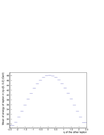
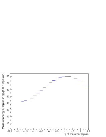
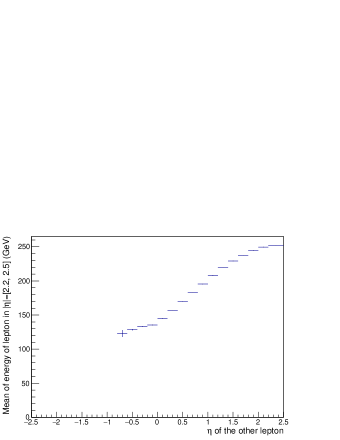
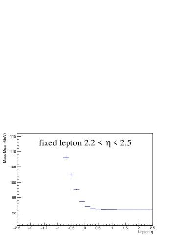
To determine parameters of $k$ and $b$, the first step of the method has to introduce enough physics constraints. It can be done by separating the $Z/\gamma^{*}\rightarrow\ell^{+}\ell^{-}$ events into subsamples based on the opening angle between leptons. At hadron collider, leptons from heavy boosted $Z$ boson decay are close to each other, and have higher energy and smaller opening angle, while leptons from almost stationary $Z$ boson decay tend to have lower energy and larger opening angle. Thus, the dilepton events can be separated into subsamples with different lepton energies by cutting on the opening angle. Since cutting on the opening angle is separating more on the $Z$ boson boost, the line shapes of dilepton mass spectrum are still good. As a result, in each separated subsample, the constraint from mean value of the dilepton mass, $\mathcal{E}(M)$, corresponds to a unique value of the mean value of lepton energy $\mathcal{E}(E_{\text{obs}})$, providing several points when determining the line in Eq. 8. Fig. 1 shows an example for the above description. Subsamples are made to contain at least one lepton in a given $\eta$ region, but have the other lepton in different $\eta$ regions, so that the leptons in the given $\eta$ region have different energies.

Figure 1: $\mathcal{E}(E)$ in separated subsamples. The Y-axis is the energy mean of the lepton in a given $\eta$ region of three examples for [0, 0.2] (top), [1.0, 1.2] (middle) and [2.2, 2.5] (bottome). The X-axis is the $\eta$ of the other lepton in the dilepton events. Each plot shows the different energy of the leptons in the given $\eta$ region. Some bins are empty because there is no event if $\Delta\eta$ between two leptons is too large.

For each $\eta$ region, there are two parameters, $k(\eta)$ and $b(\eta)$, to be determined. Thus, with a total number $N$ of $\eta$ regions involved in a dilepton sample, there are $2N$ factors in total, while the number of subsamples is $N(N-1)$. To have enough mass constraints, we must have $N(N-1)\geq 2N$. Therefore, the minimal value of $N$ is three, indicating that 6 $k(\eta)$ and $b(\eta)$ factors have to be determined together as a group with six subsamples.

We introduce a group of three $\eta$ regions denoted as $L$, $M$ and $H$. The six subsamples, according to the combination of lepton $\eta$ is $LL$, $LM$, $LH$, $MM$, $MH$ and $HH$ (e.g. $LL$ means both lepton in $L$ region, $LH$ means one lepton in $L$ and the other in $H$ region). For parameters related to the $L$ region, $k_{L}$ and $b_{L}$, $LL$, $LM$ and $LH$ events provide three constraints. For parameters related to the $M$ region, $k_{M}$ and $b_{M}$, $LM$, $MM$ and $MH$ events provide three constraints. For parameters related to the $H$ region, $k_{H}$ and $b_{H}$, $LH$, $MH$ and $HH$ events provide three constraints. The constraints can be expressed as six equations:

$$M^{2}_{\text{true}}[\alpha\beta] = M^{2}_{\text{corr}}[\alpha\beta]$$ (16)

$$= 2(b_{\alpha}+k_{\alpha}\cdot E_{\text{obs}}[\alpha])\times$$

$$(b_{\beta}+k_{\beta}\cdot E_{\text{obs}}[\beta])(1-\cos\theta)$$

where $\alpha,\beta=L,M,H$ ($LM$ and $ML$ are same, $LH$ and $HL$ are same, and $MH$ and $HM$ are same). After calculating the mean, the above constraints are equivalent to the following nine equations:

$$b_{\alpha}+k_{\alpha}\cdot\mathcal{E}(E^{\alpha}_{\alpha\beta}[\text{obs}]) = \mathcal{E}(E^{\alpha}_{\alpha\beta}[\text{true}])$$ (17)

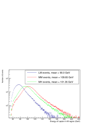
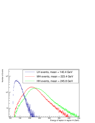
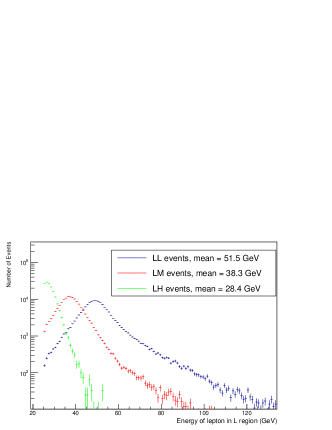
where $E^{\alpha}_{\alpha\beta}[\text{corr}]$ and $E^{\alpha}_{\alpha\beta}[\text{true}]$ ($\alpha,\beta=L,M,H$) are the energy after correction and its corresponding true value of the leptons appears in region $\alpha$ while the other lepton appears in region $\beta$. Since we only have six mass constraints, the nine equations in Eq. 17 are not independent of each other. Fig. 2 shows an example of designed $\eta$ regions, $L=[0,0.2]$, $M=[-1.6,-1.4]$ and $H=[-2.5,-2.2]$, and the different lepton energies in subsamples.

Figure 2: Energy spectrum of the lepton in $Z\rightarrow\ell^{+}\ell^{-}$ events. The X-axis is the energy of the lepton in $L=[0,0.2]$ (top), $M=[-1.6,-1.4]$ (middle) and $H=[-2.5,-2.2]$ (bottom) region. The three colors corresponds to the $\eta$ region of the other lepton. Spectrum in one plot are scaled to the same normalization.

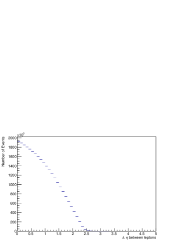
The more significant $\mathcal{E}(E^{\alpha}_{\alpha\beta})$ ($\alpha,\beta=L,M,H$) differ from each other, the higher sensitivity we have in the determination of $k$ and $b$ parameters. To make $\mathcal{E}(E^{\alpha}_{\alpha\beta})$ significantly differ, $L$, $M$ and $H$ regions should have large $\Delta\eta$ between them. But it reduces the statistics in subsamples, as shown in Fig. 3. At LHC, difference between $\mathcal{E}(E^{\alpha}_{\alpha\beta})$ is more important than statistics, because the data sample of dilepton events is large enough.

Figure 3: Distribution of $|\Delta\eta|$ between leptons in $Z/\gamma^{*}\rightarrow\ell^{+}\ell^{-}$ events.

II.2 II-B. Correlation

Eq. 16 in principle provides enough constraints. A naive try is to determine $k$ and $b$ values by minimizing a $\chi^{2}$ defined as:

$$\chi^{2}=\sum_{\alpha\beta}\frac{\left[\mathcal{E}(M_{\text{corr}}[\alpha\beta])-\mathcal{E}(M_{\text{true}}[\alpha\beta])\right]^{2}}{\sigma^{2}_{M}[\alpha\beta]}$$ (18)

where $\alpha,\beta=L,M,H$ refer to the six event categories. $\mathcal{E}(M_{\text{corr}}[\alpha\beta])$ is the mean of the mass spectrum after calibration in each event category. $\mathcal{E}(M_{\text{true}}[\alpha\beta])$ is the reference mean of the mass spectrum. $\sigma_{M}[\alpha\beta]$ is the uncertainty of the observed mass mean, which is statistically dominated by the data subsamples.

However a fit always stops at a very large $\chi^{2}$ value and gives unreasonable values for $k$ and $b$. It is simply caused by correlation between parameters, especially the correlation between $k$ and $b$ in the same $\eta$ region. The correlation gives many extreme points (but not minimal points) of $\chi^{2}$ value in the $k$-$b$ six dimension space, while only one of them is the physics solution of $k$ and $b$ values. In another word, it is difficult to provide a reasonable range for the unknown factors in the fit. This difficulty could be solved by using some advanced fit method, but is time-consuming. As data accumulates very fast at hadron colliders, we need to have a procedure that can reduce the correlation easily and fast.

II.3 II-C. Reduce the correlation

The idea to reduce the correlation is to construct a relationship between $k$ and $b$ parameters in each $\eta$ region. In this relationship, quantities except $k$ and $b$ should be known, so that $b$ can be expressed using $k$. Eq. I.2 is a good choice. But as discussed, it holds as an approximation. Here we do a better derivation.

For events with both leptons in the same $\eta$ region, the mass can be re-written as:

$$M^{2}_{\text{true}} = 2(b+kE^{\text{obs}}_{1})(b+kE^{\text{obs}}_{2})(1-\cos\theta_{12})$$ (19)

$$= \left(k+\frac{b}{E^{\text{obs}}_{1}}\right)\cdot\left(k+\frac{b}{E^{\text{obs}}_{2}}\right)\cdot M^{2}_{\text{obs}}$$

Because $\mathcal{E}(X\cdot Y)=\mathcal{E}(X)\cdot\mathcal{E}(Y)+cov(X,Y)$ and $\mathcal{E}(X^{2})=\mathcal{E}(X)^{2}+\mathcal{D}(X)$ (where $cov$ means co-variance and $\mathcal{D}$ means variance), we have

$$\mathcal{E}(M^{2}_{\text{true}}) = \mathcal{E}(M_{\text{true}})^{2}+\mathcal{D}(M_{\text{true}}),$$

$$\mathcal{E}(M^{2}_{\text{true}}) = \mathcal{E}\left[\left(k+\frac{b}{E^{\text{obs}}_{1}}\right)\cdot\left(k+\frac{b}{E^{\text{obs}}_{2}}\right)\cdot M^{2}_{\text{obs}}\right]$$ (20)

$$= \mathcal{E}\left[\left(k+\frac{b}{E^{\text{obs}}_{1}}\right)\left(k+\frac{b}{E^{\text{obs}}_{2}}\right)\right]\cdot\mathcal{E}(M_{\text{obs}})^{2}$$

$$+\mathcal{E}\left[\left(k+\frac{b}{E^{\text{obs}}_{1}}\right)\left(k+\frac{b}{E^{\text{obs}}_{2}}\right)\right]\cdot\mathcal{D}(M_{\text{obs}})$$

$$+cov\left[\left(k+\frac{b}{E^{\text{obs}}_{1}}\right)\left(k+\frac{b}{E^{\text{obs}}_{2}}\right),M^{2}_{\text{obs}}\right].$$

When $b=0$, Eq. II.3 leads to a conclusion that ratio of mass is consistent with ratio of energy:

$$\frac{\mathcal{E}(E_{\text{true}})}{\mathcal{E}(E_{\text{obs}})}=\frac{\mathcal{E}(M_{\text{true}})}{\mathcal{E}(M_{\text{obs}})}.$$

When $b\neq 0$, a correction $\epsilon$ has to be added due to the co-variance between $M$, $E_{1}$ and $E_{2}$:

$$\frac{\mathcal{E}(E_{\text{true}})}{\mathcal{E}(E_{\text{obs}})} = \frac{\mathcal{E}(M_{\text{true}})}{\mathcal{E}(M_{\text{obs}})}+\epsilon$$

$$\mathcal{E}(E_{\text{true}}) = b+k\cdot\mathcal{E}(E_{\text{obs}})$$ (21)

$$= \mathcal{E}(E_{\text{obs}})\cdot\left[\frac{\mathcal{E}(M_{\text{true}})}{\mathcal{E}(M_{\text{obs}})}+\epsilon\right].$$

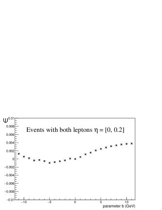
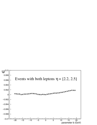
Note that all calculations of $\mathcal{E}$ are based on an ensemble of events where both leptons are in the same $\eta$ region. $b$ can be expressed using Eq. II.3. $\mathcal{E}(E_{\text{obs}})$, $\mathcal{E}(M_{\text{obs}})$ and $\mathcal{E}(M_{\text{true}})$ can be easily observed or known. $\epsilon$ is in principle also known. However calculating co-variance between energy and mass spectrum is too troublesome. Instead, we can leave $\epsilon$ as a free parameter in the final fit. Fitting for $k$ and $\epsilon$ is much easier than fitting for $k$ and $b$, because with mass constraints used in Eq. II.3, $\epsilon$ is reduced to a very small value. The estimated values of $\epsilon$ as a function of $b$ are shown in Fig. 4. $\epsilon$ is 10 times smaller than $b/E$. So the correlation between $k$ and $\epsilon$ causes no trouble in the fit because we can give $\epsilon$ a fit range much smaller than the range for $b$.

Figure 4: Estimated value of $\epsilon$ as a function of $b$ in events with both leptons $\eta=[0,0.2]$ (top) and $\eta=[2.2,2.5]$ (bottom). In the top plot, lepton energy is around 50 GeV. When $b$ is changing in a range of $\pm 10$ GeV, the fitting range for $b/E\sim\pm 0.2$ while $|\epsilon|<\pm 0.002$. In the bottom plot, lepton energy is around 200 GeV. When $b$ is changing in a range of $\pm 20$ GeV, the fitting range for $b/E\sim\pm 0.1$ while $|\epsilon|<0.001$.

One may say, why not observe $\mathcal{E}(E_{\text{true}})$ and $\mathcal{E}(E_{\text{obs}})$, so that the relationship between $b$ and $k$ is directly provided as the first row in Eq. II.3? As discussed in section I-A, difference between $\mathcal{E}(E_{\text{true}})$ and $\mathcal{E}(E_{\text{obs}})$ is determined not only by energy scale, but also PDFs and QCD calculation. An example is shown in Tab. 1. Two samples of $pp\rightarrow Z/\gamma^{*}\rightarrow\ell^{+}\ell^{-}$ events are generated with different PDF sets randomly chosen from the NNPDF NNPDF . The mean of lepton energy differs by $3\%$, while the mean of dilepton mass only differs by $0.006\%$. Therefore, we do not observe $\mathcal{E}(E_{\text{true}})$ and $\mathcal{E}(E_{\text{obs}})$ simultaneously. Instead, any comparison between observation and its corresponding truth value should be done with mass.

PDF	Mean of	Mean of
	dilepton mass	lepton energy
NNPDF3.1	90.693 GeV	246.199 GeV
NLO No. 397
NNPDF3.1	90.688 GeV	254.442 GeV
LO No. 36

Table 1: Mean of dilepton mass and lepton energy in $p\bar{p}\rightarrow Z/\gamma^{*}\rightarrow\ell^{+}\ell^{-}$ events generated using two different PDF sets. Events are generated in mass range from 60 to 130 GeV.

II.4 II-D. Fit procedure

The fit procedure is described in this section. From the relationship between $k$ and $b$ parameters observed using $LL$, $MM$ and $HH$ events, we have

$$b_{L} = -\mathcal{E}(E^{L}_{LL}[\text{obs}])\cdot k_{L}$$

$$+\mathcal{E}(E^{L}_{LL}[\text{obs}])\cdot\left[\frac{\mathcal{E}(M_{LL}[\text{true}])}{\mathcal{E}(M_{LL}[\text{obs}])}+\epsilon_{L}\right]$$

$$b_{M} = -\mathcal{E}(E^{M}_{MM}[\text{obs}])\cdot k_{M}$$

$$+\mathcal{E}(E^{M}_{MM}[\text{obs}])\cdot\left[\frac{\mathcal{E}(M_{MM}[\text{true}])}{\mathcal{E}(M_{MM}[\text{obs}])}+\epsilon_{M}\right]$$

$$b_{H} = -\mathcal{E}(E^{H}_{HH}[\text{obs}])\cdot k_{H}$$ (22)

$$+\mathcal{E}(E^{H}_{HH}[\text{obs}])\cdot\left[\frac{\mathcal{E}(M_{HH}[\text{true}])}{\mathcal{E}(M_{HH}[\text{obs}])}+\epsilon_{H}\right].$$

Then, values of $k_{L}$, $k_{M}$, $k_{H}$, $\epsilon_{L}$, $\epsilon_{M}$ and $\epsilon_{H}$ can be determined by a fit minimizing the $\chi^{2}$ defined as in Eq. 18. As discussed in section II-C, the fit range for $\epsilon$ is much narrower than that for $b$.

III III. Generator level test

The method is tested at the generator level. A $pp\rightarrow Z/\gamma^{*}\rightarrow\ell^{+}\ell^{-}$ sample is generated with statistics equivalent to the integrated luminosity of $\sim 35$ fb^-1 at 13 TeV LHC. As described in section II, the calibration is determining $k$ and $b$ in three $\eta$ regions as a group. Table 2 is an example of bins for $\eta=[-2.5,2.5]$.

Group	$H$ region	$M$ region	$L$ region
1	[-2.5, -2.2]	[-1.6, -1.4]	[0, 0.2]
2	[-2.2, -2.0]	[-1.4, -1.2]	[0.2, 0.4]
3	[-2.0, -1.8]	[-1.2, -1.0]	[0.4, 0.6]
4	[-1.8, -1.6]	[-1.0, -0.8]	[0.6, 0.8]
5	[2.2, 2.5]	[1.4, 1.6]	[-0.2, 0]
6	[2.0, 2.2]	[1.2, 1.4]	[-0.4, -0.2]
7	[1.8, 2.0]	[1.0, 1.2]	[-0.6, -0.4]
8	[1.6, 1.8]	[0.8, 1.0]	[-0.8, -0.6]

Table 2: An example of binning in the calibration procedure. 24 regions in 8 groups fully cover the $\eta$ region from $-2.5$ to $+2.5$.

For each $\eta$ region, the energy of the lepton is shifted by $k$ and $b$ parameters:

$$E_{\text{shift}}(\eta)=k_{\eta}\cdot E(\eta)+b_{\eta}.$$ (23)

Values of $k_{\eta}$ are given by a uniform distribution in a region of 0.97 to 1.03. Values of $b_{\eta}$ are given by a uniform distribution in a region of $-3$ to $+3$ GeV. Then, a $p_{T}>25$ GeV cut is applied to the lepton. A nominal $pp\rightarrow Z/\gamma^{*}\rightarrow\ell^{+}\ell^{-}$ sample is also generated without any energy shift. The calibration method described in section II is applied to the energy shifted sample to match with the nominal sample.

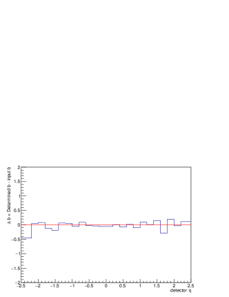
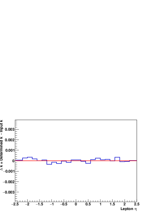
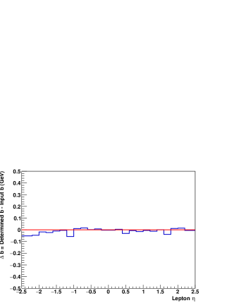
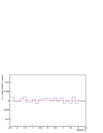
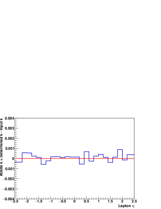
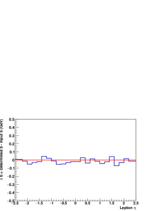
Fig. 5 shows the difference between the input values of $k_{\eta}$ and $b_{\eta}$ and their fitted values using the calibration procedure. As we can see, $\delta k$ and $\delta b$ are very small, randomly located around 0. The relative uncertainties in $\delta k$ and $\delta b$ are smaller than 0.002, which is dominated by the statistics of the two samples.

Figure 5: $\delta k$ and $\delta b$ between the input values and the fitted values. relative uncertainty is smaller than 0.002. $\delta b$ is in measurement of GeV.

The uncertainty of the calibration can be estimated using Eq. 14:

$$\frac{\Delta E}{E}=\delta k\cdot\left[1-\frac{E}{\mathcal{E}(E)}\right]$$ (24)

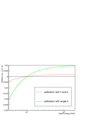
where $\mathcal{E}(E)\sim 100$ GeV in dilepton events. The energy dependence in the classic calibration with single parameter in Eq. 11 is reduced from $b/\mathcal{E}(E)$ to $\delta k$. The relative uncertainty as a function of $E$ is shown in Fig. 6.

Figure 6: Relative uncertainty $\Delta E/E$ as a function of $E$. For calibration with both $k$ and $b$ factors, running speed is set to $\delta k=0.002$. For calibration with single scaling $k$ factor, the ignored factor is set to $b=1$ GeV.

Note that in the new calibration method, the dependence $\delta k$ can be further reduced with larger data sample, while in the single scaling calibration, the running speed $b/\mathcal{E}(E)$ cannot be reduced. To prove the uncertainty is dominated by statistical fluctuations, a generator level test using larger samples with 1000M events has been done. $\delta k$ and $\delta b$ from the large sample test are shown in Fig. 7. The relative uncertainty is smaller than 0.0005. The improvement from 0.002 to 0.0005 is consistent with the increase of statistics from 72M to 1000M ($\sqrt{1000/72}$).

Figure 7: $\delta k$ and $\delta b$ between the input values and the fitted values in large sample test. Relative uncertainty is smaller than 0.0005. $\delta b$ is in measurement of GeV.

The calibration should be independent of PDFs. Another test using 1000 M large sample has been done to estimate the effect from PDFs. In this test, the energy shifted sample is generated with NNPDF3.1 NLO No. 397, while the nominal sample is generated with NNPDF3.1 LO No. 36. Fig. 8 shows the $k$ and $b$ values determined using the PDF-differed samples. Even though these two PDF sets cause large energy difference as listed in Tab. 1, $\delta k$ and $\delta b$ are still less than $0.0006$, which is consistent with uncertainties in Fig. 7 This test indicates the systematic uncertainty from PDFs is negligible compared to the statistical uncertainty.

Figure 8: $\delta k$ and $\delta b$ between the input values and the fitted values using PDF-differed samples. relative uncertainty is smaller than 0.0006. $\delta b$ is in measurement of GeV.

IV IV. Alternative Methods

IV.1 IV-A. Forward lepton calibration

The procedure described in section II and section III uses dilepton events with both leptons in the same $\eta$ region. However at hadron collider experiments, dilepton events with both leptons in forward region with high $\eta$ are difficult to be reconstructed. The coverage of the inner detector, the quality and efficiency of lepton measurement are also limited due to the large contribution of backgrounds. To perform a forward lepton calibration, the calibration method is modified so that we do not need events with both leptons in forward region.

Assume the central region ($C$) where lepton $\eta$ is relatively low has already been calibrated using the calibration method in section III. Separate it into multiple subregions, denoted as $C_{i}$. For a given forward region ($F$) with high $\eta$, the mass of dilepton events $C_{i}F$, with one lepton in $F$ and the other in $C_{i}$, is written as:

$$E^{F}_{\text{corr}} = b_{F}+k_{F}\cdot E^{F}_{\text{obs}}$$

$$M^{2}_{\text{true}}[C_{i}F] = M^{2}_{\text{corr}}[C_{i}F]$$ (25)

$$= 2E^{C_{i}}E^{F}_{\text{obs}}(1-\cos\theta_{iF})$$

$$= 2E^{C_{i}}(b_{F}+k_{F}\cdot E^{F}_{\text{obs}})(1-\cos\theta_{iF})$$

where $E^{C_{i}}$ is considered to be well calibrated. Then we can have a linear relationship between $b_{F}$ and $k_{F}$:

$$b_{F} = \mathcal{A}\cdot k_{F}+\mathcal{B}$$ (26)

$$= \mathcal{E}(-E^{F}_{\text{obs}})\cdot k_{F}+\mathcal{E}\left[\frac{M^{2}_{\text{true}}[C_{i}F]}{M^{2}_{\text{obs}}[C_{i}F]}\cdot E^{F}_{\text{obs}}\right]$$

where $\mathcal{A}$ and $\mathcal{B}$ are determined by the mean of observed $F$ lepton energy $E^{F}_{\text{obs}}$, the observed mass $M_{\text{obs}}[C_{i}F]$ and its true value $M_{\text{true}}[C_{i}F]$. Note that a mass constraint only provides $\mathcal{E}(M_{\text{true}}[C_{i}F])$, not $M_{\text{true}}[C_{i}F]$ for each individual event. So $\mathcal{B}$ is affected by covariance between $M_{\text{obs}}[C_{i}F]$, $M_{\text{true}}[C_{i}F]$ and $E^{F}_{\text{obs}}$. It can be observed in an alternative way. Fix $k_{F}$ with a given value, then fit for the value of $b_{F}$ by minimizing the $\chi^{2}$ defined as:

$$\chi^{2}=\frac{[\mathcal{E}(M_{\text{corr}}[C_{i}F])-\mathcal{E}(M_{\text{true}}[C_{i}F])]^{2}}{\sigma^{2}_{M}[C_{i}F]}.$$ (27)

Note that with only one factor $b_{F}$ in the fitting, one can always achieve a good fitting result with low $\chi^{2}$. Then, fix $k_{F}$ to other values and repeat the fitting for $b_{F}$. Finally we have a group of $b_{F}$-$k_{F}$ pairs where the values of $k_{F}$ are given while the values of $b_{F}$ are fitted. These pairs can be used to further fit the linear relationship between $b_{F}$ and $k_{F}$.

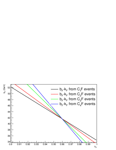
For each $C_{i}$, the relationship between $b_{F}$ and $k_{F}$ can be observed independently, with different slope $\mathcal{A}$ and offset $\mathcal{B}$. These $b_{F}$-$k_{F}$ lines should have one intersection point, corresponding to the determined value of $b_{F}$ and $k_{F}$.

A closure test is performed as an example using the 72M sample. The $F$ region is given as $2.5<\eta<3.0$. Parameters $k_{F}=0.960$ and $b_{F}=-41.651$ GeV, are applied to the $F$ lepton energy. The $C$ region is separated into four subsamples, given in Tab. 3. For each $C_{i}$, the observed slope $\mathcal{A}$ and $\mathcal{B}$ are also listed. Fig. 9 shows the four observed $b_{F}$-$k_{F}$ lines. Their intersection point corresponds to the determined values of $k_{F}=0.966$ and $b_{F}=-40.116$ GeV. Compared to the injected $k_{F}$ and $b_{F}$ value, the running factor from Eq. 14 is $\delta k_{F}=0.006$. It is much smaller than the running factor of $b_{F}/\mathcal{E}(E^{F}_{\text{obs}})\sim 40/200=0.25$ in Eq. 11 for a single factor calibration.

	$\eta$ range	$\mathcal{A}$ from $C_{i}F$(GeV)	$\mathcal{B}$ from $C_{i}F$ (GeV)
$C_{1}$	[-2.5, 0]	-177.327	211.830
$C_{2}$	[0, 0.8]	-208.678	241.918
$C_{3}$	[0.8, 2.0]	-281.295	311.607
$C_{4}$	[2.0, 2.5]	-336.097	364.201

Table 3: An example of forward lepton calibration.

Figure 9: Observed $b_{F}$-$k_{F}$ lines in each $C_{i}F$ categories. The intersection point corresponds to the determined values of $b_{F}$ and $k_{F}$.

In principle, $k_{F}$ and $b_{F}$ can be determined with two $C_{i}$ regions. But two lines always have one intersection point, even if there is bias in the $b_{F}$-$k_{F}$ relationship observation. It is good to have more than two $C_{i}$ regions, so that the calibration can be tested by checking whether these $b_{F}$-$k_{F}$ lines intersect at one point.

IV.2 IV-B. Muon calibration

Muon momentum is measured from the fitted curvature of muon tracks, which has dependence with muon charge due to detector misalignment misalignment . When charge dependence is introduced, we have 12 parameters of $k^{\pm}$ and $b^{\pm}$ in a group of $H$, $M$ and $L$ regions, but only 9 mass constraints from subsamples $H^{+}H^{-}$, $H^{+}M^{-}$, $H^{+}L^{-}$, $M^{+}H^{-}$, $M^{+}M^{-}$, $M^{+}L^{-}$, $L^{+}H^{-}$, $L^{+}M^{-}$ and $L^{+}L^{-}$. We introduce 3 additional constraints by observing variable $R$ defined as:

$$R_{L} = \frac{\mathcal{E}(E^{L^{+}}_{L^{+}L^{-}})}{\mathcal{E}(E^{L^{-}}_{L^{+}L^{-}})}$$

$$R_{M} = \frac{\mathcal{E}(E^{M^{+}}_{M^{+}M^{-}})}{\mathcal{E}(E^{M^{-}}_{M^{+}M^{-}})}$$

$$R_{H} = \frac{\mathcal{E}(E^{H^{+}}_{H^{+}H^{-}})}{\mathcal{E}(E^{H^{-}}_{H^{+}H^{-}})}$$ (28)

where $E^{\alpha^{\pm}}_{\alpha^{+}\alpha^{-}}$ $(\alpha=L,M,H)$ are energy of $\mu^{\pm}$ in events $\alpha^{+}\alpha^{-}$. The constraints can be expressed as requiring $R^{\text{corr}}_{\alpha}$ after correction to be consistent with $R^{\text{true}}_{\alpha}$ calculated from true energy mean $\mathcal{E}(E_{\text{true}})$:

$$R^{\text{obs}}_{\alpha}\rightarrow R^{\text{corr}}_{\alpha}=R^{\text{true}}_{\alpha}.$$ (29)

Note that we use the ratio of energy instead of the energy itself to avoid effects from PDFs and QCD calculation. Such effects are less significant in the ratio since energies of $\mu^{+}$ and $\mu^{-}$ are correlated.

A procedure of reducing correlations between $k^{\pm}$ and $b^{\pm}$ is still needed. The procedure is similar to the electron case with slight changes. The dimuon masses are:

$$M^{2}_{\text{true}} = 2(k^{+}E^{+}_{\text{obs}}+b^{+})(k^{-}E^{-}_{\text{obs}}+b^{-})(1-\cos\theta_{+-})$$

$$M^{2}_{\text{obs}} = 2E^{+}_{\text{obs}}E^{-}_{\text{obs}}(1-\cos\theta_{+-}).$$ (30)

Thus we have

$$\frac{M_{\text{true}}}{M_{\text{obs}}}=\sqrt{\frac{k^{+}E^{+}_{\text{obs}}+b^{+}}{E^{+}_{\text{obs}}}\cdot\frac{k^{-}E^{-}_{\text{obs}}+b^{-}}{E^{-}_{\text{obs}}}}.$$ (31)

As shown in section II-C, a correction $\epsilon$ should be added due to the covariance between $M$, $E^{+}$ and $E^{-}$ when calculating for mean values:

$$\sqrt{\frac{k^{+}\mathcal{E}(E^{+}_{\text{obs}})+b^{+}}{\mathcal{E}(E^{+}_{\text{obs}})}\cdot\frac{k^{-}\mathcal{E}(E^{-}_{\text{obs}})+b^{-}}{\mathcal{E}(E^{-}_{\text{obs}})}}=\frac{\mathcal{E}(M_{\text{true}})}{\mathcal{E}(M_{\text{obs}})}+\epsilon.$$ (32)

Defining variables of $R$ as

$$R^{\text{obs}} = \frac{\mathcal{E}(E^{+}_{\text{obs}})}{\mathcal{E}(E^{-}_{\text{obs}})}$$

$$R^{\text{true}} = \frac{k^{+}\mathcal{E}(E^{+}_{\text{obs}})+b^{+}}{k^{-}\mathcal{E}(E^{-}_{\text{obs}})+b^{-}}$$ (33)

we have:

$$k^{+}\mathcal{E}(E^{+}_{\text{obs}})+b^{+} = \mathcal{E}(E^{+}_{\text{obs}})\cdot\sqrt{\frac{R^{\text{true}}}{R^{\text{obs}}}}\cdot\left[\frac{\mathcal{E}(M_{\text{true}})}{\mathcal{E}(M_{\text{obs}})}+\epsilon\right]$$

$$k^{-}\mathcal{E}(E^{-}_{\text{obs}})+b^{-} = \mathcal{E}(E^{-}_{\text{obs}})\cdot\sqrt{\frac{R^{\text{true}}}{R^{\text{obs}}}}\cdot\left[\frac{\mathcal{E}(M_{\text{true}})}{\mathcal{E}(M_{\text{obs}})}+\epsilon\right].$$ (34)

Eq. IV.2 allows us to use $k^{\pm}$ and $\epsilon$ to represent $b^{\pm}$. These relationships can be observed using $\alpha^{+}\alpha^{-}$ events ($\alpha=L,M,H$):

$$k^{\pm}_{\alpha}\mathcal{E}(E^{\alpha^{\pm}}_{\alpha^{+}\alpha^{-}}[\text{obs}]) + b^{\pm}_{\alpha}=\mathcal{E}(E^{\alpha^{\pm}}_{\alpha^{+}\alpha^{-}}[\text{obs}])\cdot\sqrt{\frac{R^{\text{true}}_{\alpha}}{R^{\text{obs}}_{\alpha}}}$$ (35)

$$\times\left[\frac{\mathcal{E}(M_{\text{true}}[\alpha^{+}\alpha^{-}])}{\mathcal{E}(M_{\text{obs}}[\alpha^{+}\alpha^{-}])}+\epsilon_{\alpha}\right].$$

$k^{\pm}_{\alpha}$ and $\epsilon_{\alpha}$ can be further determined by minimizing the $\chi^{2}$ defined as

$$\chi^{2} = \sum_{\alpha^{+}\beta^{-}}\frac{\left[\mathcal{E}(M_{\text{corr}}[\alpha^{+}\beta^{-}])-\mathcal{E}(M_{\text{true}}[\alpha^{+}\beta^{-}])\right]^{2}}{\sigma^{2}_{M}[\alpha^{+}\beta^{-}]}$$ (36)

$$+ \sum_{\alpha^{-}\beta^{+}}\frac{\left[\mathcal{E}(M_{\text{corr}}[\alpha^{-}\beta^{+}])-\mathcal{E}(M_{\text{true}}[\alpha^{-}\beta^{+}])\right]^{2}}{\sigma^{2}_{M}[\alpha^{-}\beta^{+}]}$$

$$+ \sum_{\alpha}\frac{\left[R^{\text{obs}}_{\alpha}-R^{\text{true}}_{\alpha}\right]^{2}}{\sigma^{2}_{R}[\alpha]}$$

where $\alpha,\beta=L,M,H$ refer to nine mass constraints and three energy ratio constraints. $\sigma_{M}$ is the uncertainty on observed mass mean, and $\sigma_{R}$ is the uncertainty on $R$.

This method is tested using the 72 M samples. As an example, Twelve parameterrs of $k^{\pm}$ and $b^{\pm}$ for three $\eta$ regions, [-2.5, -2.2], [-1.6, -1.4] and [0, 0.2], are applied to shift the muon energy. Their values are randomly given. The muon calibration is applied to determine values of the factors using a nominal sample. The input values and determined values are listed in Tab. 4. The average uncertainty of $\delta k\sim 0.005$ is larger than the uncertainty in Fig. 5, because events are separated into smaller subsamples with larger statistical fluctuations. Another reason is the uncertainty $R$ variable observation using muon energy has larger uncertainties.

	Input	Determined	Input	Determined
	$k$	$k$	$b$ (GeV)	$b$ (GeV)
[0, 0.2]
$\mu^{-}$	1.0258	1.0199	2.341	2.609
$\mu^{+}$	1.0133	1.0157	2.841	2.729
[-1.6, -1.4]
$\mu^{-}$	0.9889	0.9876	-2.216	-2.005
$\mu^{+}$	0.9736	0.9783	-1.916	-2.4569
[-2.5, -2.2]
$\mu^{-}$	0.9810	0.9783	-2.761	-1.969
$\mu^{+}$	0.9706	0.9775	-1.561	-3.276

Table 4: Input values and determined values of $k^{\pm}$ and $b^{\pm}$ in $\eta$ regions of one group.

V V. Further Discussion

V.1 V-A. $\eta$-dependence in mass observation

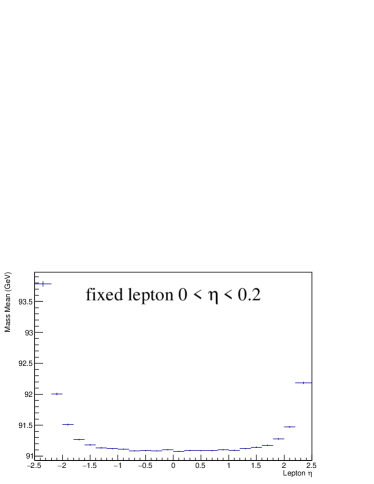
The mean value of mass spectra is a constant only in full phase space of final state leptons from $Z$ boson decay. In the calibration, dilepton events are applied with lepton $p_{T}$ and $\eta$ cuts. The mean value of dilepton mass spectrum in each subsample corresponds to a cut-phase space, thus has dependence of lepton $\eta$. When the opening angle between the two leptons in the $Z/\gamma^{*}\rightarrow\ell^{+}\ell^{-}$ events is large, at least one of the lepton $p_{T}$ is lower. Therefore a lepton $p_{T}$ cut tend to remove low mass events and keep high mass events. As a result, the mean of the mass is shifted by the cut. Such effect can be very large, as shown in Fig. 10.

To consider such effect, when performing an absolute calibration, $\mathcal{E}(M_{\text{true}})$ must be acquired from a generator-level sample with lepton $p_{T}$ and $\eta$ cut same as that applied in data and MC simulations.

Figure 10: Energy of the lepton in $Z\rightarrow\ell^{+}\ell^{-}$ events. The Y-axis is the mean of the dilepton mass spectrum with one lepton fixed in $\eta$ region [0, 0.2] (top) and [2.2, 2.5] (bottom). The X-axis is the $\eta$ of the other lepton in the dilepton events. Note that some bins are empty because there is no event if $\Delta\eta$ between two leptons is too large.

V.2 V-B. Correlation with resolution

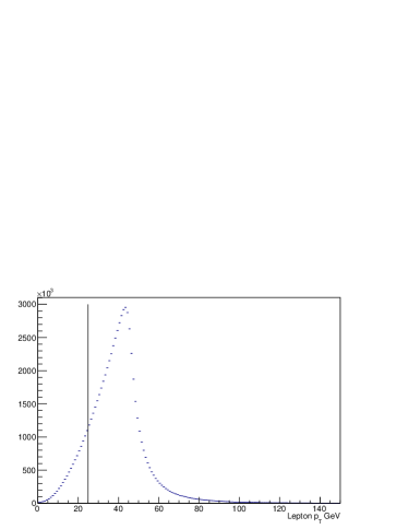
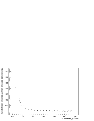
The calibration on lepton energy scale has correlation with energy resolution, which is also from lepton $p_{T}$ cut. The lepton $p_{T}$ spectra from $Z/\gamma^{*}\rightarrow\ell^{+}\ell^{-}$ events is shown in Fig. 11. Due to a peak structure, events with lepton $p_{T}$ larger than the cut value are more than events with lepton $p_{T}$ lower than than cut value. Even if the resolution itself is symmetrical, it smears more events from high $p_{T}$ to low $p_{T}$. As a result, a cut applied on the reconstructed lepton $p_{T}$ is slightly rejecting more high $p_{T}$ leptons. It will cause a non linear relationship between $E_{\text{obs}}$ and $E_{\text{true}}$ in the selected sample. It is purely a statistical effect, as if the $p_{T}$ cut is selecting data sample with bias.

Figure 11: Distribution of lepton $p_{T}$ from $Z/\gamma^{*}\rightarrow\ell^{+}\ell^{-}$ events before any $p_{T}$ cut.

Fig. 12 shows an example of the resolution effect. A $5\%$ gaussian smearing ($N(0,0.05^{2})$) is applied to the lepton energy in the $Z/\gamma^{*}\rightarrow\ell^{+}\ell^{-}$ sample. A $p_{T}>25$ GeV cut is then applied to the lepton $p_{T}$ after smearing. As we can see, the ratio of average lepton energy before and after smearing is not a constant, even if the smearing itself does not change the average of lepton energy. If the resolution is not symmetrical, such effect will be even larger. This effect has to be considered in the energy scale calibration. $\mathcal{E}(E_{\text{true}})$ and $\mathcal{E}(E_{\text{true}})$ must be observed with consistent resolution smearing, which requires a good modeling of the detector resolution.

Figure 12: Ratio of smeared lepton energy and corresponding true energy as a function of lepton energy.

VI VI. Summary

In conclusion, we described a new calibration method using $Z\rightarrow\ell^{+}\ell^{-}$ method. The new method allows offset terms in the calibration function and can precisely determine the values of the parameters. The method first introduces multiple-mass constraints by separating the $Z\rightarrow\ell^{+}\ell^{-}$ events according to the opening angle between leptons. Then, a step by step fitting procedure is used to reduce the remaining correlation between parameters. A generator level test shows that the precision of the $k$ and $b$ parameters determined by this method is around $0.2\%$, and the precision of the energy calibration is $<10^{-4}$, with a data sample equivalent to 35 fb^-1 data collected by the ATLAS or the CMS detector at the LHC 13 TeV. The uncertainty is dominated by the data sample which can be further reduced with more events. With slight modification, the calibration can be used for forward lepton calibration where dilepton events must have at least one lepton in central region, and for muon calibration where charge-dependence must be introduced. This method uses only information of the reconstructed dilepton mass. The precision is much higher than the classic single-parameter calibration. It is much faster and easier than performing a perfect detector simulation, or an advanced but time-consuming fitting technique.

VII Acknowledgements

References

• (1) G. Aad et al. (ATLAS Collaboration), Measurement of W±superscript𝑊plus-or-minusW^{\pm} and Z𝑍Z-boson production cross section in pp𝑝𝑝pp collisions at s=13𝑠13\sqrt{s}=13 TeV with the ATLAS detector, Phys. Lett. B 759 (2016) 601.
• (2) T. Sjo¨¨o\ddot{\text{o}}strand, P. Ede´´e\acute{\text{e}}n, C. Feriberg, L. Lo¨¨o\ddot{\text{o}}nnblad, G. Miu, S. Mrenna, and E. Norrbin, Comp. Phys. Commun. 135, 238 (2001). pythia version v6.323 is used throughout.
• (3) Richard D. Ball et al. (NNPDF Collaboration), Parton distributions for the LHC Run II, arXiv:1410.8849 [hep-ph] (2014).
• (4) G. Abbiendi et al. (LEP Collaborations ALEPH, DELPHI, L3 and OPAL, SLD Collaboration, LEP Electronweak Working Group, SLD Electroweak and Heavy Flavor Groups), Precision electroweak measurement on the Z𝑍Z reasonance, Phys. Rep. 427, 257 (2006).
• (5) A. Bodek, A. van Dyne, J.-Y. Han, W. Sakumoto, and A. Srelnikov, Extracting Muon Momentum Scale Corrections for Hadron Collider Experiments, Eur. Phys. J. C 72, 2194 (2012).