Predictability of sequences and subsequences with spectrum degeneracy at periodically located points

Abstract

The paper established sufficient conditions of predictability with degeneracy for the spectrum at $M$-periodically located isolated points on the unit circle. It is also shown that $m$-periodic subsequences of these sequences are also predictable if $m$ is a divisor of $M$. The predictability can be achieved for finite horizon with linear predictors defined by convolutions with certain kernels. As an example of applications, it is shown that there exists a class of sequences that is everywhere dense in the class of all square-summable sequences and such that its members can be recovered from their periodic subsequences. This recoverability is associated with certain spectrum degeneracy of a new kind.

Keywords: spectrum degeneracy, periodic spectrum gaps, subsequences, predictability.

AMS classification : 94A12, 93E10

1 Introduction

It is well known that band-limited sequences, or sequences with Z-transform vanishing on an open arc of the unit circle ${\mathbb{T}}=\{z\in{\bf C}:\ |z|=1\}$, are predictable, i.e. their future values can be estimated with arbitrarily small error from observation of their history; see e.g. the literature review in [1]. It is also known that

• A sequence is predictable if its Z-transform vanishes with a certain rate at a single point [1].

• If there are $m$-periodic spectrum gaps on ${\mathbb{T}}$ of positive measure, then $m$-periodic subsequences are predictable.

The paper established sufficient conditions of predictability with degeneracy for the spectrum at $M$-periodically located isolated points on the unit circle (Theorem 2.2). In addition, it shows that $m$-periodic subsequences of these sequences are also predictable if $m$ is a divisor of $M$ (Corollary 2.7). This is a new result for the case where either $M>m$ or the spectrum does not have gaps of positive measure.

It is shown that the corresponding predictability can be achieved for finite horizon with linear predictors defined by convolutions with certain kernels that were presented explicitly.

This result implies sequences are predictable if they are formed as a combination of sequences with periodically located isolated points on ${\mathbb{T}}$ where Z-transform is vanishing (Theorem 2.11). These compound sequences feature predictability even if their Z-transform is separated from zero on ${\mathbb{T}}$.

As an example of applications, it is shown that there exists a class of sequences that is everywhere dense in the class of all square-summable sequences and such that its members can be recovered from their periodic subsequences (Theorems 3.4-3.7). These theorems represents a modification of the related result obtained in [3].

Some definitions and notations

We denote by $L_{2}(D)$ the usual Hilbert space of complex valued square integrable functions $x:D\to{\bf C}$, where $D$ is a domain.

We denote by ${\mathbb{Z}}$ the set of all integers. Let ${\mathbb{Z}}_{q}^{+}=\{k\in{\mathbb{Z}}:\ k\geq q\}$, let ${\mathbb{Z}}_{q}^{-}=\{k\in{\mathbb{Z}}:\ k\leq q\}$, and let ${\mathbb{Z}}_{[a,b]}=\{k\in{\mathbb{Z}}:\ a\leq a\leq b\}$.

For a set $G\subset{\mathbb{Z}}$ and $r\in[1,\infty]$, we denote by $\ell_{r}(G)$ a Banach space of complex valued sequences $\{x(t)\}_{t\in G}$ such that $\|x\|_{\ell_{r}(G)}\stackrel{{\scriptstyle{\scriptscriptstyle\Delta}}}{{=}}\left(\sum_{t\in G}|x(t)|^{r}\right)^{1/r}<+\infty$ for $r\in[1,+\infty)$, and $\|x\|_{q(G)}\stackrel{{\scriptstyle{\scriptscriptstyle\Delta}}}{{=}}\sup_{t\in G}|x(t)|<+\infty$ for $r=\infty$. We denote $\ell_{r}=\ell_{r}({\mathbb{Z}})$.

We denote by $B_{r}(\ell_{2})$ the closed ball of radius $r>0$ in $\ell_{2}$.

Let $D^{c}\stackrel{{\scriptstyle{\scriptscriptstyle\Delta}}}{{=}}\{z\in{\bf C}:|z|>1\}$, and let ${\mathbb{T}}\stackrel{{\scriptstyle{\scriptscriptstyle\Delta}}}{{=}}\{z\in{\bf C}:|z|=1\}$.

For $x\in\ell_{2}$, we denote by $X={\cal Z}x$ the Z-transform

$$X(z)=\sum_{k=-\infty}^{\infty}x(k)z^{-k},\quad z\in{\bf C}.$$

Respectively, the inverse Z-transform $x={\cal Z}^{-1}X$ is defined as

$$x(k)=\frac{1}{2\pi}\int_{-\pi}^{\pi}X\left(e^{i\omega}\right)e^{i\omega k}d\omega,\quad k=0,\pm 1,\pm 2,....$$

For $x\in\ell_{2}$, the trace $X|_{\mathbb{T}}$ is defined as an element of $L_{2}({\mathbb{T}})$.

Let ${\rm H}^{r}(D^{c})$ be the Hardy space of functions that are holomorphic on $D^{c}$ including the point at infinity with finite norm

$$\|h\|_{{\rm H}^{r}(D^{c})}=\sup_{\rho>1}\|h(\rho e^{i\omega})\|_{L_{r}(-\pi,\pi)},$$

$r\in[1,+\infty]$.

For

n∈Z_1^+$and$β∈(-π,π]$,let$R_n,β$bethesetofall$ω∈(-π,π]$suchthat$e^iωn=e^iβ$,i.e.\@@eqnarray R_{n,\beta}=\{\omega_{n,\beta,k}\}_{k=0,...,n-1},\quad\hbox{where}\quad\omega_{n,\beta,k}=\frac{2\pi k-\beta}{n}.\par\par Inthispapers,wefocusonprocesseswithoutspectrumgapsofpositivemeasureon$T$butwithspectrumgapsatisolatedperiodicpointson$T$whereZ-transformsvanisheswithacertainrate.\par Let$L¿1$begiven.(Infact,wecantake$L=1$forallresultsbelowexceptTheorem\ref{ThDeg},wherewerequirethat$L¿1$issufficientlylarge;thisisrathertechnicalconditionsthatisusedintheproof.)\par For$β∈(-π,π],q¿1,c¿0$,and$ω∈(-π,π]$,set\@@eqnarray\varrho(\omega,\widetilde{\omega},q,c)=\frac{1}{L}\max\left(L,\exp\frac{c}{|e^{i\omega}-e^{i\widetilde{\omega}}|^{q}}\right).\par\par\par\par For$r¿0$,let$X_n,β(q,c,r)$bethesetofall$x∈ℓ_2$suchthat\@@eqnarray\max_{k=0,1,...,n-1}\int_{-\pi}^{\pi}|X\left(e^{i\omega}\right)|^{2}\varrho(\omega,\omega_{n,\beta,k},q,c)^{2}d\omega\leq r,\cr\ where$X=Zx$.\par Let\@@eqnarray{\cal X}_{n}\stackrel{{\scriptstyle{\scriptscriptstyle\Delta}}}{{=}}\cup_{\beta\in(-\pi,\pi],q>0,c>0,r>0}{\cal X}_{n,\beta}(q,c,r).\par\par For$m∈Z_1^+$and$s∈Z$,let$SS_m,s:ℓ_2→ℓ_2$beamappingrepresentingdecimationofasequencesuchthat$y(t)=x(t)I_{(t+s)/m∈Z}$for$y=SS_m,sx$.\par Let$ subseq​_m,s:ℓ_2→ℓ_2$beamappingrepresentingextractionofasubsequencesuchthat$^y(k)=x(km-s)$forall$k∈Z$for$^y= subseq​_m,sx$.\par Let$superseq _m,s:ℓ_2→ℓ_2$beamappingrepresentingconstructionofasupersequencesuchthat$¯x(t)=¯y(t)I_{(t+s)/m∈Z}$for$¯x=superseq _m,s¯y$.\par\par Let$^K^+$betheclassoffunctions$:Z→R$suchthat$(t)=0$for$t¡0$andsuchthat$=Z∈H^∞(D^c)$.Let$^K^-$betheclassoffunctions$:Z→R$suchthat$(t)=0$for$t¿0$andsuchthat$=Z∈H^∞(D)$.Let$^K$bethelinearspanof$^K^+∪^K^-.

2 The main results

Up to the end of this paper, we assume that we are given $m\geq 1$, $m\in{\mathbb{Z}}$.

Definition 2.1

Let ${\cal X}\subset\ell_{2}$ be a class of processes. We say that the class ${\cal X}$ is uniformly $\ell_{2}$-predictable on finite horizon if for any $\varepsilon>0$ and any integers $n>0$ (any $n<0$) there exists $\wh\in\widehat{\cal K}^{+}$ (respectively, $\wh\in\widehat{\cal K}^{-}$ for $n<0$) and $\psi\in\ell_{\infty}$ such that $\inf_{k}|\psi(k)|>0$, $\sup_{k}|\psi(k)|<+\infty$, and

$$\sum_{t\in{\mathbb{Z}}}|x(t+n)-\widehat{x}(t)|^{2}\leq\varepsilon\quad\forall x\in{\cal X},$$

where

$$\widehat{x}(t)\stackrel{{\scriptstyle{\scriptscriptstyle\Delta}}}{{=}}\psi(t)^{-1}\sum_{s\in{\mathbb{Z}}}\wh(t-s)\psi(s)x(s).$$

In Definition 2.1, the use of $\wh\in\widehat{\cal K}^{-}$ means causal extrapolation, i.e. estimation of $\widehat{x}(t+n)$ for $n>0$ is based on observations $\{x(k)\}_{k\leq t}$, and the use of $\wh\in\widehat{\cal K}^{+}$ means anti-causal extrapolation, i.e. estimation of $\widehat{x}(t+n)$ for $n<0$ is based on observations $\{x(k)\}_{k\geq t}$.

Theorem 2.2

For any $q>0$, $r>0$, $\nu\in{\mathbb{Z}}_{1}^{+}$, $\beta\in(-\pi,\pi]$, $s\in{\mathbb{Z}}$, and $\rho>0$, the class of sequences ${\cal X}_{m\nu,\beta}(q,c,r)$ is uniformly predictable on finite horizon in the sense of Definition 2.1 with $\psi(t)=e^{i\theta t}$ and $\theta=(\beta-\pi)/(m\nu)$.

2.1 Robustness of prediction

Definition 2.3

Let ${\cal X}\subset\ell_{2}$ be a set of sequences. Consider a problem of predicting $\{x(k)\}_{\in{\mathbb{Z}}_{[-M,M]}}$ using observations of noise contaminated sequences $x=\widetilde{x}+\xi$, where ${\mathbb{Z}}_{[-M,M]}=\{k\in{\mathbb{Z}},\ |k|\leq M\}$, $\widetilde{x}\in{\cal X}$, and where $\xi\in\ell_{2}$ represents a noise. Suppose that only truncated traces of observations of $\{x(k),\ k\in{\cal T}_{0},\ -N\leq k<-M\}$ available (or only traces $\{x(k),\ k\in{\cal T}_{0},\ -N\leq k<-M\}$ are available), where $N>0$ is an integer. We say that the class ${\cal X}$ allows uniform and robust prediction if, for any integer $M>0$ and any $\varepsilon>0$, there exists $\rho>0$, $N_{0}>0$, a set of sequences $\{\psi_{t}(\cdot)\}_{t\in{\mathbb{Z}}_{[-M,M]}}$ such that $\psi_{t}\in\ell_{\infty}$, $\inf_{k}|\psi_{t}(k)|>0$, $\sup_{k}|\psi_{t}(k)|<+\infty$ for any $t$, and a set $\{\wh_{t}(\cdot)\}_{t\in{\mathbb{Z}}_{[-M,M]}}\subset{\cal K}^{+}$ (or a set $\{\wh_{t}(\cdot)\}_{t\in{\mathbb{Z}}_{[-M,M]}}\subset{\cal K}^{-}$ respectively) such that

$$\max_{t\in{\mathbb{Z}}_{[-M,M]}}|x(t)-\widehat{x}(t)|\leq\varepsilon\quad\forall\widetilde{x}\in{\cal X}_{m\nu,\beta}(q,c,r),\quad\forall\xi\in B_{\rho}(\ell_{2}),$$

for any $N>N_{0}$ and for

$$\widehat{x}(t)=\psi_{t}(t)^{-1}\sum_{s\in{\cal T}_{0},\ M<|s|\leq N}\wh_{t}(t-s)\psi_{t}(s)x(s),\quad t\in{\mathbb{Z}}_{[-M,M]},$$

with $\psi_{t}(s)=e^{i\theta s}$ for all $t$ and $\theta=(\beta-\pi)/(m\nu)$.

The following theorem shows that predicting is robust with respect to noise contamination and truncation.

Theorem 2.4

For given $\nu\in{\mathbb{Z}}_{1}^{+},\beta\in(-\pi,\pi],q>0,c>0,r>0$, the class of sequences ${\cal X}_{m\nu,\beta}(q,c,r)$ allows uniform and robust prediction in the sense of Definition 2.3 with $\psi(t)=e^{i\theta t}$ and $\theta=(\beta-\pi)/(m\nu)$.

2.2 Predictability of subsequences

Definition 2.5

Let $q>0$, $\nu\in{\mathbb{Z}}_{1}^{+}$, $\beta\in(-\pi,\pi]$, $q>0$, $c>0$, $r\geq 0$, and $s\in{\mathbb{Z}}$, be given.

1. Let ${\cal Y}_{m,\nu,\beta,s}(q,c,r)$ be the set of all $y\in\ell_{2}$ such that there exists $x\in{\cal X}_{m\nu,\beta}(q,c,r)$ such that $y=\SS_{m,s}x$.

2. Let $\widehat{\cal Y}_{m,\nu,\beta,s}(q,c,r)$ be the set of all $y\in\ell_{2}$ such that there exists $x\in{\cal X}_{m\nu,\beta}(q,c,r)$ such that $\widehat{y}={subseq}\!_{m,s}x$ for $x\in{\cal X}_{m\nu,\beta}(q,c,r)$.

Lemma 2.6

${\cal Y}_{m,\nu,\beta,s}(q,c,r)\subset{\cal X}_{m\nu,\beta}(q,c,r_{1})$ for some $r_{1}=r_{1}(m,\nu,\beta,q,s,r)$.

Corollary 2.7

Let $\nu\in{\mathbb{Z}}_{1}^{+}$, $\beta\in(-\pi,\pi]$, $q>0$, $c>0$, $r\geq 0$, and $s\in{\mathbb{Z}}$, be given. Let either ${\cal X}={\cal Y}_{m,\nu,\beta,s}(q,c,r)$ or ${\cal X}=\widehat{\cal Y}_{m,\nu,\beta,s}(q,c,r)$. Then the class of sequences ${\cal X}$ is uniformly predictable on finite horizon in the sense of Definition 2.1 and allows robust uniform prediction in the sense of Definition 2.3. This predictability is robust with respect to noise contamination in the sense of Theorem 2.4.

Let

$${\cal Y}_{m,s}\stackrel{{\scriptstyle{\scriptscriptstyle\Delta}}}{{=}}\cup_{\beta\in(-\pi,\pi],\nu\in{\mathbb{Z}}_{1}^{+},q>0,c>0,r>0}{\cal Y}_{m,\nu,\beta,s}(q,c,r),\quad{\cal Y}_{m}\stackrel{{\scriptstyle{\scriptscriptstyle\Delta}}}{{=}}\cup_{s\in{\mathbb{Z}}}{\cal Y}_{m,s}$$

and

$$\widehat{\cal Y}_{m,s}\stackrel{{\scriptstyle{\scriptscriptstyle\Delta}}}{{=}}\cup_{\beta\in(-\pi,\pi],\nu\in{\mathbb{Z}}_{1}^{+},q>0,c>0,r>0}\widehat{\cal Y}_{m,\nu,\beta,s}(q,c,r),\quad\widehat{\cal Y}_{m}\stackrel{{\scriptstyle{\scriptscriptstyle\Delta}}}{{=}}\cup_{s\in{\mathbb{Z}}}\widehat{\cal Y}_{m,s}.$$

Corollary 2.8

Let either ${\cal Y}={\cal Y}_{m}$ or ${\cal Y}=\widehat{\cal Y}_{m}$. For any $p\in{\mathbb{Z}}$, any sequence $y\in{\cal X}$ is uniquely defined by its tail $\{y(k)\}_{k\in{\mathbb{Z}}^{-}_{p}}$. It is also uniquely defined by its tail $\{y(k)\}_{k\in{\mathbb{Z}}_{p}^{+}}$.

Corollary 2.9

$\ell_{2}\setminus\widehat{\cal Y}_{m}\neq\emptyset$.

Theorem 2.2 and Corollary 2.8 indicate that sequences from ${\cal Y}_{m}$ and $\widehat{\cal Y}_{m}$ feature predictability that is usually associated with spectrum degeneracy. By Lemma 2.6, it is expectable for ${\cal Y}_{m}$ since Z-transforms of sequences from ${\cal Y}_{m}$ vanish at a periodic set of point of ${\mathbb{T}}$ as was defined for sequences from ${\cal X}_{m\nu,\beta}(q,c,r)$. However, it is less expectable for sequences from $\widehat{\cal Y}_{m}$ since their Z-transforms can be actually separated from zero on ${\mathbb{T}}$.

2.3 On detecting predictable sequences

Sequences from $\widehat{\cal Y}_{m}$ are predictable; predictability of these processes is defined by certain spectrum degeneracy of their supersequences. By Corollary 2.9, there are sequences in $\ell_{2}$ that do not belong to this class.

For a given $\widehat{y}\in\ell_{2}$, the question arises if $\widehat{y}\in\widehat{\cal Y}_{m}$. The following lemma suggests an answer for this question.

Lemma 2.10

For $\widehat{y}\in\ell_{2}$ and $s\in{\mathbb{Z}}$, we have that $\widehat{y}\in\widehat{\cal Y}_{m,s}$ if and only if $y={superseq}\,_{m\nu,s}\widehat{y}\in{\cal X}_{m\nu}$ for some $\nu\in{\mathbb{Z}}_{1}^{+}$.

According to this Lemma, $\widehat{y}$ is a subsequence of a sequence $x$ with degenerate spectrum if and only if the supersequence $y$ obtained from $x$ by nullifying members not belonging to $\widehat{y}$ also has a degenerate spectrum.

2.4 Predictability of compound processes

For $m\in{\mathbb{Z}}_{1}^{+}$, $q>0$, $c>0$, $\nu=(\nu_{0},...,\nu_{m-1})\in({\mathbb{Z}}_{1}^{+})^{m}$, $\beta=(\beta_{0},...,\beta_{m-1})\in(-\pi,\pi]^{m}$, and $s\in{\mathbb{Z}}$, let ${\cal Y}^{comp}_{m,\nu,\beta,s}(q,c,r)$ be the set of all sequences $y$ such that

$$y(k)=\sum_{d=0}^{m-1}\xi_{d}\left(k+d\right){\mathbb{I}}_{\left\{\frac{k+d}{m}\in{\mathbb{Z}}\right\}},$$

where $\xi_{d}\in{\cal Y}_{m,\nu_{d},\beta_{d},s}(q,c,r)$.

Theorem 2.11

Let $m\in{\mathbb{Z}}_{1}^{+}$, $q>0$, $\nu\in({\mathbb{Z}}_{1}^{+})^{m}$, $\beta\in(-\pi,\pi]^{m}$, $q>0$, $c>0$, and $s\in{\mathbb{Z}}$, be given. Then the class of sequences ${\cal X}={\cal Y}^{comp}_{m,\nu,\beta,s}(q,c,r)$ is uniformly predictable on finite horizon in the sense of Definition 2.1 with $\psi_{t}(s)=e^{i\theta_{t}s}$ and $\theta_{t}=(\beta_{d}-\pi)/(m\nu_{d})$ if $(t+d)/m\in{\mathbb{Z}}$.

Let

$${\cal Y}^{comp}_{m,s}\stackrel{{\scriptstyle{\scriptscriptstyle\Delta}}}{{=}}\cup_{\beta\in(-\pi,\pi],\nu\in{\mathbb{Z}}_{1}^{+},q>0,c>0,r>0}{\cal Y}^{comp}_{m,\nu,\beta,s}(q,c,r),\quad{\cal Y}^{comp}_{m}\stackrel{{\scriptstyle{\scriptscriptstyle\Delta}}}{{=}}\cup_{s\in{\mathbb{Z}}}{\cal Y}^{comp}_{m,s}.$$

Corollary 2.12

For any $p\in{\mathbb{Z}}$, any sequence ${\cal Y}^{comp}_{m}$ is uniquely defined by its tail $\{y(k)\}_{k\in{\mathbb{Z}}^{-}_{p}}$. It is also uniquely defined by its tail $\{y(k)\}_{k\in{\mathbb{Z}}_{p}^{+}}$.

Corollary 2.13

$\ell_{2}\setminus{\cal Y}_{m}^{comp}\neq\emptyset$.

It can be noted that Z-transform of sequences from ${\cal Y}_{m}^{comp}$ can be separated from zero on ${\mathbb{T}}$, so their spectrum is non-degenerate in the usual sense.

3 On recovery of sequences from their subsequences

We will need some modification of Definition 3.1.

Definition 3.1

Let ${\cal X}\subset\ell_{2}$ be a class of sequences. Let $\widetilde{\cal T}\subset{\mathbb{Z}}$. We say that the class ${\cal X}$ is uniformly recoverable from observations of $x$ on $\widetilde{\cal T}$ if, for any integer $M>0$ and any $\varepsilon>0$, there exists a set of sequences $\{\psi_{t}(\cdot)\}_{t\in{\mathbb{Z}}_{[-M,M]}}$ such that $\psi_{t}\in\ell_{\infty}$, $\inf_{k}|\psi_{t}(k)|>0$, $\sup_{k}|\psi(k)|<+\infty$ for any $t$, and a set $\{\wh_{t}(\cdot)\}_{t\in{\mathbb{Z}}_{[-M,M]}}\subset\widehat{\cal K}$ such that

$$\max_{t\in{\mathbb{Z}}_{[-M,M]}}|x(t)-\widehat{x}(t)|\leq\varepsilon\quad\forall x\in{\cal X},$$

where

$$\widehat{x}(t)=\psi_{t}(t)\sum_{s\in\widetilde{\cal T}}\wh_{t}(t-s)\psi_{t}(s)x(s),\quad t\in{\mathbb{Z}}_{[-M,M]}.$$

In Definition 3.1, the use of $\wh\in\widehat{\cal K}^{-}$ means causal extrapolation, i.e. selection of $\widehat{x}(t+n)$ for $n>0$ based on observations $\{x(k)\}_{k\leq t}$, and the use of $\wh\in\widehat{\cal K}^{+}$ means anti-causal extrapolation, i.e. selection of $\widehat{x}(t+n)$ for $n<0$ based on observations $\{x(k)\}_{k\geq t}$.

A special type of spectrum degeneracy

Definition 3.2

Let $q>0$, $r>0$, $\beta\in(-\pi,\pi]$, $s\in{\mathbb{Z}}$, and $\rho>0$ be given. We say that $x\in\ell_{2}$ features braided spectrum degeneracy with parameters $m,r,\beta,s,q$ if, for $d=-m+1,...,m-1$, there exist $\nu=(\nu_{-m+1},...,\nu_{m-1})\in({\mathbb{Z}}_{1}^{+})^{2m-1}$ and $\xi_{d}\in{\cal X}_{m\nu_{d},\beta}(q,c,r)$ such that the following holds:

1. The sets $R_{m\nu_{d},\beta}$ are mutually disjoint for $d=-m+1,....,m-1$.

2. $$\xi_{d}(k)=\xi_{0}(k),\quad k\leq 0,\quad d>0$$

   $$\xi_{d}(k)=\xi_{0}(k),\quad k\geq 0,\quad d<0,$$ (2)

3. $$x(k)=\sum_{d=0}^{m-1}\xi_{d}\left(k+d\right){\mathbb{I}}_{\left\{\frac{k+d}{m}\in{\mathbb{Z}}\right\}},\quad k\geq 0,$$

   $$x(k)=\sum_{d=-m+1}^{0}\xi_{d}\left(k+d\right){\mathbb{I}}_{\left\{\frac{k+d}{m}\in{\mathbb{Z}}\right\}},\quad k\leq 0.$$ (3)

We denote by ${\cal P}_{m,\nu,\beta}(q,c,r)$ the set of all sequences $x$ with this feature, and we denote ${\cal P}_{m}=\cup_{m,\nu,\beta,r,q,c,r}{\cal P}_{m}(q,c,r)$.

Example 3.3

A possible choice of integers $\nu_{d}$ such that all sets $R_{m\nu_{d},\pi}$ are mutually disjoint is $\nu_{d}=2^{d}$ for $d\geq 0$ and $\nu_{d}=2^{2m+d-1}$ for $d<0$.

Let

$${\cal T}_{0}=\{k\in{\mathbb{Z}}:\ k/m\in{\mathbb{Z}}\},\quad {\cal T}_{0}(s)=\{k\in{\cal T}:\ |k|>s\},$$

$${\cal T}_{d}=\{k\in{\mathbb{Z}}:\ (k-d)/m\in{\mathbb{Z}},\ k>0\},\quad d=1,...,m-1,$$

$${\cal T}_{d}=\{k\in{\mathbb{Z}}:\ (k-d)/m\in{\mathbb{Z}},\ k<0\},\quad d=-m+1,...,-1.$$

Theorem 3.4

Let $\delta>0$ and $s>0$ be given, and $L>1$ be sufficiently large in the definition for $\varrho$. Then the class ${\cal P}_{m,\nu,\beta}(q,c,r)$ is uniformly recoverable from observations on ${\cal T}_{0}(s)$ in the sense of Definition 3.1.

Remark 3.5

As is seen from the proof below, Theorem 3.4 is still valid if $\widehat{\cal K}$ in Definition 3.1 is replaced by a smaller set $\widehat{\cal K}^{-}\cup\widehat{\cal K}^{+}$.

Corollary 3.6

A sequence $x\in{\cal P}_{m}$ is uniquely defined by its subsequence $\{x(km)\}_{k\in{\mathbb{Z}}}$. Moreover, for any $s>0$, a sequence $x\in{\cal P}_{m}$ is uniquely defined by its subsequence $\{x(km)\}_{k\in{\mathbb{Z}},\ |k|>s}$.

Theorem 3.7

For any $x\in\ell_{2}$ and any $\varepsilon>0$, there exists $\widehat{x}\in{\cal P}_{m,\nu,\beta}(q,c,r)$ such that

$$\|x-\widehat{x}\|_{\ell_{2}}\leq\varepsilon.$$ (4)

In other words, the set ${\cal P}_{m}$ is everywhere dense in $\ell_{2}$.

Let us compare these results with the result of [5], where a method was suggested for recovery from observations of subsequences of missing values oversampling sequences for band-limited continuous time functions. The method [5] is also applicable for general type band-limited sequences from $\ell_{2}$. The algorithm in [5] requires to observe quite large number of subsequences, and this number is increasing as the size of spectrum gap on ${\mathbb{T}}$ is decreasing. Theorems 3.4 and 3.7 ensures recoverability with just one subsequence for a class of sequences that everywhere dense in $\ell_{2}$.

Robustness of recovery

The following theorem shows that recovery of a finite part of a sequence from ${\cal P}_{m}$ from its $m$-periodic subsequence is robust with respect to noise contamination and truncation.

Theorem 3.8

Let $m,\nu,\beta,r,q,c,r$ be given. Consider a problem of recovery of the set $\{x(k)\}_{k=-M}^{M}$ from observed subsequences of noise contaminated sequences $x=\widetilde{x}+\xi$, where $M\in{\mathbb{Z}}_{0}^{+}$, $\widetilde{x}\in{\cal P}_{m,\nu,\beta}(q,c,r)$ and where $\xi\in\ell_{2}$ represents a noise. Suppose that only truncated traces of observations of $\{x(k),\ k\in{\cal T}_{0},\ M<|k|\leq N\}$ are available, where $N>0$ is an integer. Then for any integer $M>0$ and any $\varepsilon>0$, there exists $\rho>0$, $N_{0}>0$, a set of sequences $\{\psi_{t}(\cdot)\}_{t\in{\mathbb{Z}}_{[-M,M]}}$ such that $\psi_{t}\in\ell_{\infty}$, $\inf_{k}|\psi_{t}(k)|>0$, $\sup_{k}|\psi(k)|<+\infty$ for any $t$, and a set $\{\wh_{t}(\cdot)\}_{t\in{\mathbb{Z}}_{[-M,M]}}\subset\widehat{\cal K}$ such that

$$\max_{t\in{\mathbb{Z}}_{[-M,M]}}|x(t)-\widehat{x}(t)|\leq\varepsilon\quad\forall\widetilde{x}\in{\cal P}_{m,\nu,\beta}(q,c,r),\quad\forall\xi\in B_{\rho}(\ell_{2}),$$

for any $N>N_{0}$ and for

$$\widehat{x}(t)=\psi_{t}(t)\sum_{s\in{\cal T}_{0},\ M<|s|\leq N}\wh_{t}(t-s)\psi_{t}(s)x(s),\quad t\in{\mathbb{Z}}_{[-M,M]}.$$

4 Proofs

It suffices to consider prediction on $n$ steps forward with $n>0$. The case where $n<0$ can be considered similarly.

Special predicting kernels

The proofs are based on special predicting kernels and their transfer functions representing modification of kernels and transfer functions introduced in [1].

Let us introduce transfer functions and its inverse Z-transform

$$\widehat{H}_{n}(z)=\widehat{H}_{n,{m\nu}}(z)\stackrel{{\scriptstyle{\scriptscriptstyle\Delta}}}{{=}}z^{n}V(z^{{m\nu}})^{n},\quad z\in{\bf C},\qquad\widehat{h}_{n}={\cal Z}^{-1}\widehat{H}_{n},$$ (5)

where

$$V(z)\stackrel{{\scriptstyle{\scriptscriptstyle\Delta}}}{{=}}1-\exp\left[-\frac{\gamma}{z+1-\gamma^{-\widehat{r}}}\right],$$

and where $\widehat{r}>0$ and $\gamma>0$ are parameters. Functions $V$ were introduced in [1]. In the notations from [1], $\widehat{r}=2\mu/(q-1)$, where $\mu>1$ and $q>1$ are parameters; $q$ describes the required rate of spectrum degeneracy. We assume that $r$ is fixed, and we consider variable $\gamma\to+\infty$.

In the proof below, we will show that $\widehat{H}_{n}\left(e^{i\omega}\right)$ approximates $e^{in\omega}$ and therefore defines a linear $n$-step predictor with the kernel $\widehat{h}_{n}={\cal Z}^{-1}\widehat{H}_{n}$.

The case where $\beta=\pi$

Lemma 4.1

Theorem 2.2 holds for the case where $\beta=\pi$.

Proof of Lemma 4.1. The proof represents a modification of the proof from [1], where the case of $n=1$ was considered and where the spectrum degeneracy were assumed to be at a single point only. In addition, represents a modification of the proof from [3], where the case of $\beta=\pi$ was considered.

Let $\alpha=\alpha(\gamma)\stackrel{{\scriptstyle{\scriptscriptstyle\Delta}}}{{=}}1-\gamma^{-r}$. Clearly, $\alpha=\alpha(\gamma)\to 1$ as $\gamma\to+\infty$.

Let $W(\alpha)=\arccos(-\alpha)$, let $D_{+}(\alpha)=(-W(\alpha),W(\alpha))$, and let $D(\alpha)\stackrel{{\scriptstyle{\scriptscriptstyle\Delta}}}{{=}}[-\pi,\pi]\backslash D_{+}(\alpha)$. We have that $\cos(W(\alpha))+\alpha=0$, $\cos(\omega)+\alpha>0$ for $\omega\in D_{+}(\alpha)$, and $\cos(\omega)+\alpha<0$ for $\omega\in D(\alpha)$.

It was shown in D12a [1] that the following holds:

• $V(z)\in{\rm H}^{\infty}(D^{c})$ and $zV(z)\in{\rm H}^{\infty}(D^{c})$.

• $V(e^{i\omega})\to 1$ for all $\omega\in(-\pi,\pi)$ as $\gamma\to+\infty$.

• If $\omega\in D_{+}(\alpha)$ then ${\rm Re\,\!}\left(\frac{\gamma}{e^{i\omega}+\alpha}\right)>0$ and $|V\left(e^{i\omega}\right)-1|\leq 2$.

• For any $c>0$, there exists $\gamma_{0}>0$ such that, for any $\gamma\geq\gamma_{0}$,

  $$|V\left(e^{i\omega}\right)-1|\varrho(\omega,\pi,q,c)^{-1}\leq 1\quad\forall\omega\in D(\alpha).$$

Without a loss of generality, we assume below that $\gamma>\gamma_{0}$ for corresponding $c$.

Let

$$Q(\alpha)=\cup_{k=0}^{{m\nu}-1}\left(\frac{W(\alpha)+2\pi k}{{m\nu}},\frac{2\pi-W(\alpha)+2\pi k}{{m\nu}}\right),\qquad Q_{+}(\alpha)=[-\pi,\pi]\setminus Q(\alpha).$$

From the properties of $V$, it follows that the following holds.

• $V(z^{{m\nu}})^{n}\in{\rm H}^{\infty}(D^{c})$ and $\widehat{H}_{n}(z)=z^{n}V(z^{{m\nu}})^{n}\in{\rm H}^{\infty}(D^{c})$.

• $V\left(e^{i\omega{m\nu}}\right)\to 1$ and $\widehat{H}_{n}\left(e^{i\omega}\right)\to e^{in\omega}$ for all $\omega\in(-\pi,\pi]\setminus R_{{m\nu}}$ as $\gamma\to+\infty$.

• $${\rm Re\,\!}\left(\frac{\gamma}{e^{i\omega{m\nu}}+\alpha}\right)>0,\quad\left|V\left(e^{i\omega{m\nu}}\right)-1\right|\leq 1\quad\forall\omega\in Q_{+}(\alpha).$$

• For any $c>0$, there exists $\gamma_{0}>0$ such that, for any $\gamma>\gamma_{0}$,

  $$|V\left(e^{i\omega{m\nu}}\right)-1|\varrho(\omega,\omega_{{m\nu},\pi,k},q,c)^{-1}d\omega\leq 1\quad\forall\omega\in Q(\alpha),\forall k=0,1,...,{m\nu}-1.$$

Let $p=\{p_{l}\}\in{\bf R}^{n}$ be such that $a^{n}-1=\sum_{l=0}^{n}p_{l}(a-1)^{l}$. In this case,

$$V\left(e^{i\omega{m\nu}}\right)^{n}-1=\sum_{l=0}^{n}p_{l}(V\left(e^{i\omega{m\nu}}\right)-1)^{l}$$

and

$$|V\left(e^{i\omega{m\nu}}\right)^{n}-1|\leq\sum_{l=0}^{n}|p_{l}||V\left(e^{i\omega{m\nu}}\right)-1|^{l}.$$

Furthermore, we have that there exists $C_{1}=C_{1}(n)>0$ such that

$$\varrho(\omega,\omega_{{m\nu},\pi,k},q,c)^{-n/2}\leq C_{1}(n)\varrho(\omega,\omega_{{m\nu},\pi,k},q,c)^{-l/2}\forall k=0,1,...,{m\nu}-1,\quad l=1,...,n.$$

By the choice of the function $\varrho$ and by property (iii), it follows that, for any $c>0$, there exists $\gamma_{0}>0$ and $C=C(n)>0$ such that, for any $\gamma>\gamma_{0}$,

$$|V\left(e^{i\omega{m\nu}}\right)^{n}-1|\varrho(\omega,\omega_{{m\nu},\pi,k},q,n)^{-n/2}d\omega\leq C(n)\quad\forall\omega\in(-\pi,\pi],\quad\forall k=0,1,...,{m\nu}-1.$$

This implies that the following analog of the property (b4) holds.

• For any $c>0$, there exists $\gamma_{0}>0$ and $C=C(n)>0$ such that, for any $\gamma>\gamma_{0}$,

  $$|V\left(e^{i\omega{m\nu}}\right)^{n}-1|\varrho(\omega,\omega_{{m\nu},\pi,k},q,c)^{-1/2}d\omega\leq C(n)\quad\forall\omega\in(-\pi,\pi],\quad\forall k=0,1,...,{m\nu}-1.$$

Clearly, $\alpha=\alpha(\gamma)\to 1$ and ${\rm mes\,\!}\,Q(\alpha)\to 0$ as $\gamma\to+\infty$. It follows that, for any $c>0$,

$$\|\varrho(\omega,\omega_{{m\nu},\pi,k},q,c)^{-1/2}\|_{L_{2}(Q(\alpha))}\to 0\quad\hbox{as}\quad\gamma\to+\infty\quad\forall k=0,1,...,{m\nu}-1.$$ (6)

For $c>0$ and $r\geq 0$, consider an arbitrary $x\in{\cal X}_{m\nu,\pi}(q,c,r)$. We denote $X\stackrel{{\scriptstyle{\scriptscriptstyle\Delta}}}{{=}}{\cal Z}x$ and $\widehat{X}\stackrel{{\scriptstyle{\scriptscriptstyle\Delta}}}{{=}}\widehat{H}_{n}\,\!X$.

Let $x_{n}(t)\stackrel{{\scriptstyle{\scriptscriptstyle\Delta}}}{{=}}x(t+n)$ and $X_{n}\stackrel{{\scriptstyle{\scriptscriptstyle\Delta}}}{{=}}{\cal Z}x_{n}$. In this case, $X_{n}(z)=z^{n}X(z)$. We have that

$$\|X_{n}\left(e^{i\omega}\right)-\widehat{X}\left(e^{i\omega}\right)\|_{L_{1}(-\pi,\pi)}=I_{1}+I_{2},$$

where

$$I_{1}=\int_{Q(\alpha)}|X_{n}\left(e^{i\omega}\right)-\widehat{X}\left(e^{i\omega}\right)|d\omega,\qquad I_{2}=\int_{Q_{+}(\alpha)}|X_{n}\left(e^{i\omega}\right)-\widehat{X}\left(e^{i\omega}\right)|d\omega.$$

By the assumption, (1) holds. Hence

$$I_{1}=\|\widehat{X}\left(e^{i\omega}\right)-X_{n}\left(e^{i\omega}\right)\|_{L_{1}(Q(\alpha))}=\|(\widehat{H}_{n}\left(e^{i\omega}\right)-e^{i\omega n})X\|_{L_{1}(Q(\alpha))}$$

$$\leq\sum_{k=0}^{{m\nu}-1}\|(V\left(e^{i\omega{m\nu}}\right)^{n}-1)\varrho(\omega,\omega_{{m\nu},\pi,k},q,c)^{-1/2}\|_{L_{2}(Q(\alpha))}\|X\left(e^{i\omega}\right)\varrho(\omega,\omega_{{m\nu},\pi,k},q,c)^{1/2}\|_{L_{2}(-\pi,\pi)}.$$

By the properties of $V$, it follows that $I_{1}\to 0$ as $\gamma\to+\infty$ uniformly over $x\in{\cal X}_{m\nu,\pi}(q,c,r)$.

Let us estimate $I_{2}$. We have that

$$I_{2}=\int_{Q_{+}(\alpha)}|(e^{i\omega n}-\widehat{H}_{n}\,\!\left(e^{i\omega}\right))X\left(e^{i\omega}\right)|d\omega\leq\int_{Q_{+}(\alpha)}|e^{i\omega n}(1-V\left(e^{i\omega{m\nu}}\right)^{n})X\left(e^{i\omega}\right)|d\omega$$

$$\leq\|1-V\left(e^{i\omega{m\nu}}\right)^{n}\|_{L_{2}(Q_{+}(\alpha))}\|X\left(e^{i\omega}\right)\|_{L_{2}(-\pi,\pi)}.$$

Further, ${\mathbb{I}}_{Q_{+}(\alpha)}(\omega)|1-V\left(e^{i\omega{m\nu}}\right)^{n}|\to 0$ a.e. as $\gamma\to+\infty$. By the properties of $V$,

$${\mathbb{I}}_{Q_{+}(\alpha)}(\omega)|V\left(e^{i\omega{m\nu}}\right)^{n}-1|\leq 2^{n}\sum_{l=0}^{n}|p_{l}|.\quad\forall\gamma:\ \gamma>\gamma_{0}.$$

From Lebesgue Dominance Theorem, it follows that $\|V\left(e^{i\omega{m\nu}}\right)^{n}-1\|_{L_{2}(Q_{+}(\alpha))}\to 0$ as $\gamma\to+\infty$. It follows that $I_{1}+I_{2}\to 0$ uniformly over $x\in{\cal X}_{m\nu,\beta}(q,c,r)$. Hence

$$\sup_{k\in{\mathbb{Z}}}|x(k+n)-\widehat{x}(k)|\to 0\quad\hbox{as}\quad\gamma\to+\infty\quad\hbox{uniformly over}\quad x\in{\cal X}_{m\nu,\beta}(q,c,r),$$ (7)

where the process $\widehat{x}$ is the output of the linear predictor defined by the kernel $\widehat{h}_{n}={\cal Z}^{-1}\widehat{H}_{n}$ as

$$\widehat{x}(k)\stackrel{{\scriptstyle{\scriptscriptstyle\Delta}}}{{=}}\sum^{k}_{p=-\infty}\widehat{h}_{n}(k-p)x(p).$$ (8)

Hence the predicting kernels $\widehat{h}_{n}={\cal Z}^{-1}\widehat{H}_{n}\,\!$ constructed for $\gamma\to+\infty$ are such as required. This completes the proof of Lemma 4.1, i.e. the proof of Theorem 2.2 for the case where $\beta=\pi$.

The case where $\beta\in(-\pi,\pi]$

We are now in the position to complete the proof of Theorem 2.2 for an arbitrarily selected $\beta\in(-\pi,\pi]$

Proof of Theorem 2.2. We have that $R_{m\nu,\beta}=\{\omega_{m\nu,\beta,k}\}_{k=0,1,...,m\nu-1}$, where

$$\omega_{m\nu,\beta,k}=\frac{\beta-2\pi k}{m\nu},\quad k=0,1,...,m\nu-1.$$

Let $\theta\stackrel{{\scriptstyle{\scriptscriptstyle\Delta}}}{{=}}(\beta-\pi)/(m\nu)$. We have that

$$\omega_{m\nu,\pi,k}=\omega_{m\nu,\beta,k}-\theta,\quad k=0,1,...,m\nu-1.$$

Let us select

$$\psi(t)\stackrel{{\scriptstyle{\scriptscriptstyle\Delta}}}{{=}}e^{i\theta t},\qquad x_{\beta}(t)\stackrel{{\scriptstyle{\scriptscriptstyle\Delta}}}{{=}}\psi(t)x(t),\qquad t\in{\mathbb{Z}}.$$

Let $x\in{\cal X}_{m\nu,\beta}(q,c,r)$ for some $q>0$ and and integer $\nu>0$. Let $X_{\beta}={\cal Z}x_{\beta}$ and $X={\cal Z}x$. In this case,

$$X_{\beta}\left(e^{i\omega}\right)=\sum_{k\in{\mathbb{Z}}}e^{-i\omega k}x_{\beta}(k)=\sum_{k\in{\mathbb{Z}}}e^{-i\omega k}\psi(k)x(k)$$

$$=\sum_{k\in{\mathbb{Z}}}e^{-i\omega k+i\theta k}x(k)=X\left(e^{i\omega-i\theta}\right).$$

We have that

$$X_{\beta}\left(e^{i\omega_{m\nu,\pi,k}}\right)=X\left(e^{i\omega_{m\nu,\pi,k}-i\theta}\right)=X\left(e^{i\omega_{m\nu,\beta,k}}\right)=0,\quad k=0,1,...,m\nu-1.$$

Hence $x_{\beta}\in{\cal X}_{m\nu,\pi}(q,c,r)$. As we have established above, $x_{\beta}$ is predictable in the sense of Definition 2.1. Let $\widehat{h}_{n}$ be the corresponding predicting kernel which existence is required by Definition 2.1 for the case where $\psi(t)\equiv 1$ such that the approximation $\widehat{x}_{\beta}(t)$ of $x_{\beta}(t+n)$ is given by

$$\widehat{x}_{\beta}(t)=\sum_{k=-\infty}^{t}\widehat{h}_{n}(t-k)y_{\beta}(k).$$

These kernels were constructed in the proof of Theorem 2.2 above for the special case $\beta=\pi$. It follows that

$$\widehat{x}(t)=\psi(t)^{-1}\sum_{k=-\infty}^{t}\widehat{h}_{n}(t-k)\psi(t)x_{(}k).$$

This completes the proof of Theorem 2.2. $\Box$

Proof of Theorem 2.4. It suffices to show that the error for recovery a singe term $x(n)$ for a given integer $n>0$ from the sequence $\{x(mk)\}_{k\in{\mathbb{Z}},\,k\leq 0}$ can be made arbitrarily small is a well-posed problem; the proof for a finite set of values to recover is similar.

The case where $n<0$ and $\{x(mk)\}_{k\in{\mathbb{Z}},\,k\geq 0}$ are observable can be considered similarly.

We assume that $N>n$.

Let us consider an input sequence $x\in\ell_{2}$ such that

$$x=\widetilde{x}+\eta,$$ (9)

where $\eta(k)=\xi(k){\mathbb{I}}_{\{|k|\leq N\}}-\widetilde{x}(k){\mathbb{I}}_{\{|k|>N\}}$. In this case, (9) gives that $x(k)=(\widetilde{x}(k)+\xi(k)){\mathbb{I}}_{\{|k|\leq N\}}$.

Let $X={\cal Z}x$, and let ${\cal N}\stackrel{{\scriptstyle{\scriptscriptstyle\Delta}}}{{=}}{\cal Z}\eta$, and let $\sigma=\|{\cal N}\left(e^{i\omega}\right)\|_{L_{2}(-\pi,\pi)}$; this parameter represents the intensity of the noise.

Let us assume first that $\beta=\pi$.

Let an arbitrarily small $\varepsilon>0$ be given. Assume that the parameters $(\gamma,\widehat{r})$ of $\widehat{H}_{n}$ in (5) with $\nu=\nu_{d}$ are selected such that

$$|\bar{x}(n)-\bar{x}(0)|\leq\varepsilon/2\quad\forall\bar{x}\in{\cal X}_{m\nu,\beta}(q,c,r),$$ (10)

for $\bar{x}={\cal Z}^{-1}(\widehat{H}_{n}\bar{X})$ and $\bar{X}={\cal Z}\bar{x}$. The kernel $\widehat{h}_{n}$ produces an estimate $\bar{x}(0)$ of based on observations of $\{\bar{x}(km)\}_{k\leq 0}$.

Let $\widetilde{x}\stackrel{{\scriptstyle{\scriptscriptstyle\Delta}}}{{=}}{\cal Z}^{-1}(\widehat{H}_{n}\widetilde{X})$, where $\widetilde{X}={\cal Z}\widetilde{x}$. By (10), we have that

$$|\widetilde{x}(0)-\widetilde{x}(n)|\leq\varepsilon/2.$$

Let $\widehat{x}\stackrel{{\scriptstyle{\scriptscriptstyle\Delta}}}{{=}}{\cal Z}^{-1}(\widehat{H}X)$, where $X={\cal Z}x$. We have that $\widehat{x}=\widetilde{x}+{\cal Z}^{-1}(\widehat{H}{\cal N})$ and

$$|\widehat{x}(0)-x(n)|\leq|\widetilde{x}(0)-x(n)|+|{\cal Z}^{-1}(\widehat{H}{\cal N})(0)|\leq\varepsilon/2+E_{\eta},$$

where

$$E_{\eta}\stackrel{{\scriptstyle{\scriptscriptstyle\Delta}}}{{=}}\frac{1}{2\pi}\|(\widehat{H}\left(e^{i\omega}\right)-e^{i\omega n}){\cal N}\left(e^{i\omega}\right)|\|_{L_{1}(-\pi,\pi)}\leq\sigma(\kappa+1),$$

and where

$$\kappa\stackrel{{\scriptstyle{\scriptscriptstyle\Delta}}}{{=}}\sup_{\omega\in[-\pi,\pi]}|\widehat{H}_{n}\left(e^{i\omega}\right)|.$$

We have that $\sigma\to 0$ as $N\to+\infty$ and $\|\xi\|_{\ell_{2}(-N,N)}\to 0$. If $N$ is large enough and $\|\xi\|_{\ell_{2}(-N,N)}$ is small enough such that $\sigma(\kappa+1)<\varepsilon/2$, then $|\widehat{x}(0)-x(n)|\leq\varepsilon$. This completes the proof of Theorem 2.4 for the case where $\beta=\pi$.

The prove for the case where $\beta\neq\pi$ follows from the case where $\beta=\pi$, since the processes $x(t),\bar{x}(t),\widetilde{x}(t),\widehat{x}(t),\widetilde{x}(t),$ presented in the proof with $\beta=\pi$ will be simply converted to processes $e^{-i\theta t}x(t),e^{-i\theta t}\bar{x}(t),e^{-i\theta t}\widehat{x}(t),e^{-i\theta t}\widetilde{x}(t)$, for $\theta=(\beta-\pi)/(m\nu)$, similarly the proof of Theorem 2.2. $\Box$

Remark 4.2

By the properties of $\widehat{H}_{n}$, we have that $\kappa\to+\infty$ as $\gamma\to+\infty$. This implies that error (4) will be increasing if $\widehat{\varepsilon}\to 0$ for any given $\sigma>0$. This means that, in practice, the predictor should not target too small a size of the error, since in it impossible to ensure that $\sigma=0$ due inevitable data truncation.

Proof of Lemma 2.6. Let $y\in{\cal Y}_{m,\nu,\beta,s}(q,c,r)$ for some $m,\nu,\beta,\delta,s,r$. By the definitions, there exists $x\in{\cal X}_{m\nu,\beta}(q,c,r)$ such that $y=\SS_{m,s}x$. It suffices to prove that $y\in{\cal X}_{m\nu,\beta}(q,c,r_{1})$ for some $r_{1}=r_{1}(m,\nu,\beta,\delta,s,r)$.

Let us consider the case where $s=0$. In this case, $Y={\cal Z}y$ can be represented as

$$Y\left(e^{i\omega}\right)=\frac{1}{m}\sum_{k=1}^{m}X\left(e^{i\omega+i\omega_{m,0,k}}\right).$$

(See e.g. [4] , pp. 167-168). To prove that $y\in{\cal X}_{m\nu,\beta}(q,c,r_{1})$ for some $r_{1}>0$, it suffices to show that

$$e^{i(\omega_{m\nu,\beta,l}+\omega_{m,0,k})}\in\{e^{i\omega_{m\nu,\beta,d}}\}_{d=0,1,..,m\nu-1},\quad k,l\in{\mathbb{Z}}.$$ (11)

We have that

$$\omega_{m\nu,\beta,l}=\frac{2\pi l-\beta}{m\nu},\quad\omega_{m,0,k}=\frac{2\pi k}{m}.$$

Hence for all $k,l\in{\mathbb{Z}}$ we have that

$$e^{i(\omega_{m\nu,\beta,l}+\omega_{m,0,k})}=\exp\left(i\frac{2\pi l-\beta}{m\nu}+i\frac{2\pi k}{m}\right)=\exp\left(i\frac{2\pi l-\beta+2\pi km}{m\nu}\right).$$

This implies that (11) holds.

Consider now a general case of $s\in{\mathbb{Z}}$.

Consider operator $S:\ell_{2}\to\ell_{2}$ such that $(Sx)(t)=x(t+s)$. Let $x_{s}=Sx$ and $y_{s}=Sy$. For $y=\SS_{m,s}x$, we have that $y_{s}=Sy=\SS_{m,0}x_{s}$. Clearly, $x_{s}\in{\cal X}_{m\nu,\beta}(q,c)$. As was proved above, $y_{s}\in{\cal X}_{m\nu,\beta}(q,c,r_{1})$ for some $r_{1}>0$. Hence $y\in{\cal X}_{m\nu,\beta}(q,c,r_{1})$. This completes the proof of Lemma 2.6.$\Box$

The proof of Corollary 2.7. For ${\cal X}={\cal Y}_{m,\nu,\beta,s}(q,c,r)$, the proof follows immediately from the proof of Lemma 2.6. The proof for ${\cal X}={\cal Y}_{m,\nu,\beta,s}(q,c,r)$ follows immediately from the observation that there is a natural bijection between ${\cal Y}_{m}$ and $\widehat{\cal Y}_{m}$; one may simply represent $\widehat{y}\in\widehat{\cal Y}$ as an element of ${\cal Y}$ and establish predictability by application of the predictor derived above for sequences from ${\cal Y}_{m}$. $\Box$

Proof of Corollary 2.8. It suffices to prove that if $y\in{\cal Y}_{m}$ such that $y(k)=0$ for $k\leq s$, then $y(k)=0$ for $k>q$ for all $q\in{\mathbb{Z}}$. By the predictability established by Theorem 2.7, for a process $y\in{\cal Y}_{m}$ such that $y(k)=0$ for $k\leq s$, it follows that $y(k+1)=0$; we obtain this by letting $\gamma\to+\infty$ in (5). Similarly, we obtain that $y(k+2)=0$. Repeating this procedure, we obtain that $y(k)=0$ for all $k\in{\mathbb{Z}}$. $\Box$

Corollary 2.9 follows immediately from Corollary 2.8. $\Box$

Lemma 2.10. Let $\widehat{y}\in\widehat{\cal Y}_{m,s}$ and let $\widehat{Y}={\cal Z}\widehat{y}$. By the definitions, $\widehat{y}={subseq}\!_{m,s}x$ for some $x\in{\cal X}_{m\nu,\beta}(q,c,r_{1})$ and $\nu,\beta,r_{1}$. Let $s=0$, and let $Y(z)\stackrel{{\scriptstyle{\scriptscriptstyle\Delta}}}{{=}}\widehat{Y}(z^{m})$. By Lemma 2.6, $y\in{\cal X}_{m\nu,\beta}(q,c,r_{1})$. At the same time, $y={superseq}\,_{m,0}\widehat{y}$. Then the proof follows.

then, follows fro $\Box$

The proof of Theorem 2.11, Corollary 2.12, and Corollary 2.13 repeats the proofs above with minor modifications, and will be omitted here.

Proof for Example 3.3. It suffices to show that $\omega_{\mu(m,d_{1}),k}\neq\omega_{\mu(m,d_{2}),l}$ if $d_{1}\neq d_{2}$ for all $k,l\in{\mathbb{Z}}$ , where $\omega_{n,k}=\frac{2\pi k-\pi}{n}$ are the roots of the equation $e^{inw}=-1$. Suppose that $\omega_{\mu(m,d_{1}),k}=\omega_{\mu(m,d_{2}),l}$ for some $k,l\in{\mathbb{Z}}$ for $d_{2}=d_{1}+r$, for some $d_{1},d_{2}\in\{-m+1,...,m-1\}$ such that $a\stackrel{{\scriptstyle{\scriptscriptstyle\Delta}}}{{=}}d_{2}-d_{1}>0$. In this case, the definitions imply that

$$\frac{2k-1}{2^{d_{1}}}=\frac{2l-1}{2^{d_{2}}}.$$

This means that $2^{a}(2k-1)=2l-1$ which implies that the number $2^{a}(2k-1)$ is odd. This is impossible since we had assumed that $a>0$. Hence the sets $R_{m\nu_{d},\beta}$ are mutually disjoint for different $d$. This completes the proof for Example 3.3. $\Box$

We will need an extended version of Definition 3.1.

Definition 4.3

Let $P$ be a finite subset of ${\mathbb{Z}}$ with $N>0$ elements, Let ${\cal X}$ be a class of ordered sets $\{x_{p}\}_{p\in P}\subset(\ell_{2})^{N}$. Let a set ${\cal I}\subset{\mathbb{Z}}$ be given, and let ${\cal I}(M)={\cal I}\setminus{\mathbb{Z}}_{[-M,M]}$. We say that the class $\bar{\cal Y}$ is uniformly recoverable from observations of $x_{0}$ on $\widetilde{\cal I}$ if, for any integer $M>0$ and any $\varepsilon>0$, there exists a set $\{\wh_{p,t}(\cdot)\}_{p\in P,t\in{\mathbb{Z}}_{[-M,M]}}\subset\widehat{\cal K}$ such that

$$\max_{p\in P,\ t\in{\mathbb{Z}}_{[-M,M]}}|x_{p}(t)-\widehat{x}_{p}(t)|\leq\varepsilon\quad\forall x\in{\cal X},$$

where

$$\widehat{x}_{p}(t)=\sum_{s\in{\cal I}(M)}\wh_{p,t}(t-s)x_{0}(s).$$

Let us introduce mappings ${\cal M}_{d}:\ell_{2}\to\ell_{2}$ for $d\in{\mathbb{Z}}_{[-m+1,m-1]}=\{-m+1,...,m-1\}$ such that, for $x\in\ell_{2}$, the sequence $x_{d}={\cal M}_{d}x$ is defined by insertion of $|d|$ new members equal to $x(0)$ as the following:

$$\hphantom{}\hbox{(i)}\,\,\,\,x_{0}=x;\hphantom{xxxxx}\hphantom{x_{d}(k)=x(0),\quad k=0,1,...,d,\quad k<0}\,\,$$

$$\hphantom{}\hbox{(ii)\,\, for}\quad d>0:\quad\hphantom{xxxxx}x_{d}(k)=x(k),\quad k<0,$$

$$\hphantom{xxxxx}x_{d}(k)=x(0),\quad k=0,1,...,d,$$

$$\hphantom{xxxxx}x_{d}(k)=x(k-d),\quad k\geq d+1;$$

$$\hphantom{}\hbox{(iii) \,\, for}\quad d<0:\quad\hphantom{xxxxx}x_{d}(k)=x(k),\quad k>0,$$

$$\hphantom{xxxxx}x_{d}(k)=x(0),\quad k=d,d+1,...,0,$$

$$\hphantom{xxxxx}x_{d}(k)=x(k-d),\quad k\leq d-1.$$

Proof of Theorem 3.4. Let $\nu_{d}>0$ be some integers $d\in{\mathbb{Z}}_{[-m+1,m-1]}=\{-m+1,...,m-1\}$. Let $\widetilde{\cal Y}_{d}$ be the set of $\xi_{d}=\SS_{m,0}x_{d}$, where $x_{d}={\cal M}_{d}x$, for all $x\in{\cal P}_{m,\nu,\beta}(q,c,r)$.

Let $\widetilde{\cal Y}(\delta)$ be the set of all ordered sets $\{\xi_{d}\}_{d=-m+1}^{m-1}$ such that $\xi_{d}\in\widetilde{\cal Y}_{d}(\delta)$.

By Lemma 4.1, the sets $\widetilde{\cal Y}_{d}(\delta)$ are uniformly predictable in the sense of Definition 2.1. It follows that, for any $s\in{\mathbb{Z}}^{+}$ and $d\geq 0$, the sets $\widetilde{\cal Y}_{d}(\delta)$ are uniformly recoverable in the sense of Definition 3.1 from observations of $\{\xi_{d}(k)\}$ on $\{k\in{\mathbb{Z}}:\ k\leq-s\}$. Clearly, time direction can be reversed and therefore it can be concluded that, for $d<0$ and any $s\in{\mathbb{Z}}$, the sets $\widetilde{\cal Y}_{d}(\delta)$ are uniformly recoverable in the sense of Definition 3.1 from observations of $\{\xi_{d}(k)\}$ on $\{k\in{\mathbb{Z}}:\ |k|\geq s\}$. By the structure of $\xi_{d}=\SS_{m,0}x_{d}$, it follows that it sufficient to use observations of $\xi_{d}$ on $\{k\in{\mathbb{Z}}:\ k/m\in{\mathbb{Z}},\ k\leq-s\}$ only for $d\geq 0$ and, respectively, observations of $\xi_{d}$ on $\{k\in{\mathbb{Z}}:\ k/m\in{\mathbb{Z}},\ k\geq s\}$ only for $d<0$.

By the definitions, we have for $d>0$ that $\xi_{d}(k)=\xi_{0}(k)$ for $k\leq 0$. For $d<0$, we have that $\xi_{d}(k)=\xi_{0}(k)$ for $k\geq 0$. Hence, for any $s>0$, the set $\widetilde{\cal Y}(\delta)$ is uniformly recoverable in the sense of Definition 4.3 (with $\psi_{p}\equiv 1$) from observations of $\xi_{0}$ on the set ${\cal T}_{0}(s)=\{k\in{\mathbb{Z}}:\ k/m\in{\mathbb{Z}},\ |k|\geq s\}$.

By the definitions again, we have that $\xi_{0}(km)=x(km)$ for all $k\in{\mathbb{Z}}$. For $d>0$, we have that $\xi_{d}(km-d)=x(km-d)$ for $k\geq 1$ and $\xi_{d}(km)=x(km)$ for $k\leq 0$. For $d<0$, we have that $\xi_{d}(km-d)=x(km-d)$ for $k\leq-1$ and $\xi_{d}(km)=x(km)$ for $k\geq 0$. Hence $x$ is uniformly recoverable in the sense of Definition 3.1 from from observations of $x$ on ${\cal T}_{0}(s)$. This completes the proof of Theorem 3.4. $\Box$

Proof of Theorem 3.7. In the proof below, we consider $d\in{\mathbb{Z}}_{[-m+1,m-1]}=\{-m+1,...,m-1\}$.

Let $x\in\ell_{2}$ be arbitrarily selected and let $x_{d}\stackrel{{\scriptstyle{\scriptscriptstyle\Delta}}}{{=}}{\cal M}_{d}x$.

We assume that all $m\nu_{d}$ are different for different $d$.

Let $Y_{d}\stackrel{{\scriptstyle{\scriptscriptstyle\Delta}}}{{=}}X_{0}-X_{d}$ and $\xi_{d}={\cal Z}^{-1}Y_{d}$, where $X_{d}={\cal Z}x_{d}$. Since $x_{d}(k)=x_{0}(k)$ for $k\leq 0$ and $d>0$, and $x_{d}(k)=x_{0}(k)$ for $k\geq 0$ and $d<0$, it follows that $\xi_{d}(k)=0$ for $k\leq 0$ and $d>0$, and $\xi_{d}(k)=0$ for $k\geq 0$ and $d<0$. In addition, $Y_{0}\equiv 0$ and $\xi_{0}\equiv 0$.

Further, let $D=\{k\in{\mathbb{Z}}:\ |k|\leq m-1,\ k\neq 0\}$, and let

$$A(\omega)=\prod_{d=-m+1}^{m-1}\prod_{k=0}^{m\nu_{d}-1}\varrho(\omega,\omega_{m\nu_{d},\beta,k},q,c)^{-1},\quad\alpha_{d}(\omega)=\prod_{k=0}^{m\nu_{d}-1}[1-\varrho(\omega,\omega_{m\nu_{d},\beta,k},q,c)^{-1}].$$

We have that, for any $(L,\widehat{r},c)$, for large enough $\gamma$,

$$(a_{d}(\omega)-1)\varrho(\omega,\omega_{m\nu_{d},\beta,k},q,c)\equiv 1\quad k=0,1,...,\nu_{d}-1.$$ (12)

We assume that $\gamma,L,\widehat{r},c$ are selected such that (12) holds.

Let

$$\widehat{X}_{0}\left(e^{i\omega}\right)\stackrel{{\scriptstyle{\scriptscriptstyle\Delta}}}{{=}}X_{0}\left(e^{i\omega}\right)A(\omega)+\sum_{p\in D}Y_{p}\left(e^{i\omega}\right)a_{p}(\omega).$$

We have that $\widehat{x}_{0}\in{\cal X}_{md_{0},\beta}(q,c,r)$, where $\widehat{x}_{0}={\cal Z}^{-1}\widehat{X}_{0}$.

Furthermore, by the definitions,

$$\widehat{X}_{d}\left(e^{i\omega}\right)=X_{d}\left(e^{i\omega}\right)+\widehat{X}_{0}\left(e^{i\omega}\right)-X_{0}\left(e^{i\omega}\right)=X_{0}\left(e^{i\omega}\right)A(\omega)+W_{d}\left(e^{i\omega}\right),$$

where

$$W_{d}\left(e^{i\omega}\right)=X_{d}\left(e^{i\omega}\right)+\sum_{p\in D}[X_{0}\left(e^{i\omega}\right)-X_{p}\left(e^{i\omega}\right)]a_{d}(\omega)-X_{0}\left(e^{i\omega}\right).$$

For large enough $L>0$, the function $\varrho$ takes the value one on the most part of ${\cal T}$, with some isolated peaks. Because of this, we have that

$$a_{p}\left(e^{i\omega}\right)\varrho(\omega,\omega_{m\nu_{d},\beta,k},q,c)=0\quad\hbox{a.e.},\quad p\neq d,\quad k=0,1,...,\nu_{d}-1.$$

By the choice of $A\left(e^{i\omega}\right)$, it follows for all $d$ that

$$\max_{k=0,1,...,m\nu_{d}-1}\int_{-\pi}^{\pi}|X_{0}\left(e^{i\omega}\right)A(\omega)|^{2}\varrho(\omega,\omega_{m\nu_{d},\beta,k},q,c)^{2}d\omega\leq r,$$ (13)

where $X={\cal Z}x$.

Let us show that, for large enough $\gamma$,

$$\max_{k=0,1,...,m\nu_{d}-1}\int_{-\pi}^{\pi}|W_{d}\left(e^{i\omega}\right)|^{2}\varrho(\omega,\omega_{m\nu_{d},\beta,k},q,c)^{2}d\omega\leq r,$$ (14)

where $X={\cal Z}x$. We have that

$$W_{d}\left(e^{i\omega}\right)=X_{d}\left(e^{i\omega}\right)-X_{0}\left(e^{i\omega}\right)+\sum_{p\in D}[X_{0}\left(e^{i\omega}\right)-X_{p}\left(e^{i\omega}\right)]a_{p}(\omega)$$

$$=Y_{d}\left(e^{i\omega}\right)(a_{d}(\omega)-1)+\sum_{p\in D,\ p\neq d}Y_{p}\left(e^{i\omega}\right)a_{p}(\omega).$$

By (12), it follows that (13) and (14) holds. Hence

$$\max_{k=0,1,...,m\nu_{d}-1}\int_{-\pi}^{\pi}|X_{d}\left(e^{i\omega}\right)|^{2}\varrho(\omega,\omega_{m\nu_{d},\beta,k},q,c)^{2}d\omega\leq r$$ (15)

and $x_{d}\in{\cal X}_{m\nu_{d},\beta}(q,c,r)$ for all $d$.

In addition, it was shown above that $\widehat{x}_{d}(k)=\widehat{x}_{0}(k)$, for $k\leq 0$ and $d>0$, and $\widehat{x}_{d}(k)=\widehat{x}_{0}(k)$, for $k\geq 0$ and $d<0$. Let $\widehat{x}$ be defined by (3), where $\xi_{d}=\widehat{x}_{d}$. By the definitions, it follows that $\widehat{x}\in{\cal P}_{m,\nu,\beta}(q,c,r)$.

Further, assume that $q>1$ is fixed and $c\to 0+$. Clearly,

$$\|a_{p}\|_{L_{2}(-\pi,\pi)}\to 0,\quad\|A\|_{L_{2}(-\pi,\pi)}\to 1\quad\hbox{as}\quad c\to 0+.$$

It follows that

$$\|\widehat{X}_{0}\left(e^{i\omega}\right)-X_{0}\left(e^{i\omega}\right)\|_{L_{2}(-\pi,\pi)}\to 0,$$

$$\|\widehat{X}_{d}\left(e^{i\omega}\right)-X_{d}\left(e^{i\omega}\right)\|_{L_{2}(-\pi,\pi)}\to 0\quad\hbox{as}\quad c\to 0+.$$

It follows that

$$\|\widehat{x}_{d}-x_{d}\|_{\ell_{2}}\to 0\quad\hbox{as}\quad c\to 0.$$ (16)

By the definitions, it follows that

$$\widehat{x}(k)-x(k)=\widehat{x}_{d}(k+d)-x_{d}(k+d),\quad k\geq 0,\quad d\geq 0,\quad(k+d)/m\in{\mathbb{Z}},$$

and

$$\widehat{x}(k)-x(k)=\widehat{x}_{d}(k+d)-x_{d}(k+d),\quad k<0,\quad d<0,\quad(k+d)/m\in{\mathbb{Z}}.$$

Then (4) follows from (16). This completes the proof of Theorem 3.7. $\Box$

Proof of Theorem 3.8 follows from Theorem 2.4 applied to the prediction of the corresponding subsequences. $\Box$

Some properties of predicting kernels

Proposition 4.4

1. The predicting kernels $\widehat{h}_{n}$ are real valued,

2. The predicting kernels $\widehat{h}_{n}$ are quite sparse:

   $$\widehat{h}_{n}(k)=0\quad\hbox{if either}\quad(k+n)/(m\nu)\notin{\mathbb{Z}}\quad\hbox{or}\quad k<mn-n.$$ (17)

Proof. To prove (i), it suffices to observe that $\widehat{H}_{n}\,\!\left(\bar{z}\right)=\overline{\widehat{H}_{n}\,\!\left(z\right)}$. Let us prove (ii). By the choice of $V$, it follows that $|V(z)|\to 0$ as $|z|\to+\infty$. Hence $v(0)=0$ for $v={\cal Z}^{-1}V$ and

$$V(z^{m\nu})=z^{-{m\nu}}v(1)+z^{-2{m\nu}}v(2)+z^{-3{m\nu}}v(3)+...$$

Clearly, we have that

$$V(z^{m\nu})^{n}=z^{-n{m\nu}}w(1)+z^{-(n+1){m\nu}}w(2)+z^{-(n+2){m\nu}}w(3)+...,$$

where $w={\cal Z}^{-1}(W)$ for $W(z)=V(z)^{n}$. Hence

$$\widehat{H}_{n}(z^{m\nu})=z^{n}V(z^{m\nu})^{n}=z^{n-n{m\nu}}w(1)+z^{n-(n+1){m\nu}}w(2)+z^{n-(n+2){m\nu}}w(3)+...$$

$$=z^{n-n{m\nu}}\widehat{h}(n{m\nu}-n)+z^{n-(n+1){m\nu}}\widehat{h}((n+1){m\nu}-n)+z^{n-(n+2){m\nu}}\widehat{h}((n+2){m\nu}-n)+...$$

Hence (17) holds. This completes the proof of Proposition 4.4. $\Box$

5 On numerical implementation

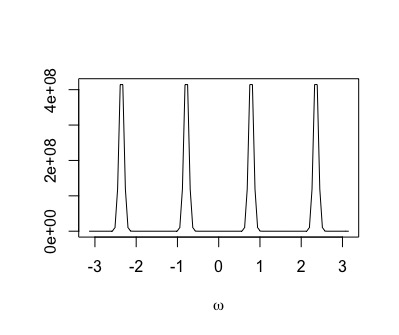
Our numerical experiments show that $\|\widehat{h}_{n}\|_{\ell_{\infty}}$ is growing very fast as $\gamma$ is increasing. For the case of relatively small $\gamma\sim 2$, some experiments were done in [2]. These experiments demonstrated that it is possible to achieve small but noticeable improvement of the prediction accuracy for autoregressions in stochastic setting. In the present paper, we attempted to improve approximation using larger $\gamma$. The main challenge here is that $\|\widehat{h}_{n}\|_{\ell_{\infty}}$ is growing very fast as is increasing very fast as $\gamma$ is increasing.

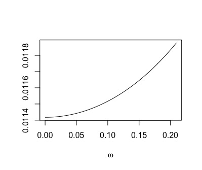
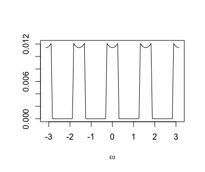
For example, we calculated for $n=2$, $r=1.2$, the kernel $\widehat{h}_{n}$ for different choices of $\gamma$ using standard integration in R. We obtained that $\|\widehat{h}_{n}\|_{\ell_{\infty}}=239,190$ for $\gamma=3$, that $\|\widehat{h}_{n}\|_{\ell_{\infty}}=2,985,964\cdot 10^{29}$ for $\gamma=6$, and that $\|\widehat{h}_{n}\|_{\ell_{\infty}}=2,475,003\cdot 10^{122}$. for $\gamma=10$. Figures 3 and 3 shows the distance $|\widehat{H}_{2}\left(e^{i\omega}\right)-e^{2i\omega}|$ from the transfer function $e^{2i\omega}$ of the ideal two-step predictor for $\gamma=3$.

This makes calculations with large $\gamma$

The values of $\widehat{h}_{n}$ of this magnitude are being coded in a standard computer programm with a large error; this generates a large error for the prediction. Potentially, application of more precise computational technique with an adequate number of digits for representation for large numbers.

The theorems presented above focus on processes without spectrum gaps of positive measure on ${\mathbb{T}}$. However, for numerical examples, we considered more special processes with periodic spectrum gaps of a positive measure ${\mathbb{T}}$ defined as the follwing.

For $\delta>0$, $\beta\in(-\pi,\pi]$, $\widehat{\omega}\in(-\pi,\pi]$, and $n\in{\mathbb{Z}}_{1}^{+}$, let

$$J(\widehat{\omega},\delta)=\{\omega\in(-\pi,\pi]:\quad|e^{i\omega}-e^{i\widehat{\omega}}|\leq\delta\},\quad J_{n,\beta}(\delta)=\cup_{k=0}^{n}J\left(\omega_{n,\beta,k},\delta\right).$$

Let ${\cal V}_{n,\beta}(\delta,r)$ be the set of all $x\in B_{r}(\ell_{2})$ such that $X\left(e^{i\omega}\right)=0$ for a.e. $\omega\in J_{n,\beta}(\delta)$, where $X={\cal Z}x$. These processes have periodic spectrum gaps of positive measure on ${\mathbb{T}}$.

Clearly, ${\cal V}_{n,\beta}(\delta,r)\subset{\cal X}_{n,\beta}(q,c,r_{1})$ for some $r_{1}=r_{1}(r,q,c,\delta,n)$, and there exists $C=(r,q,c,\delta,n)>0$ such that

$$\int_{-\pi}^{\pi}|X\left(e^{i\omega}\right)|^{2}d\omega\leq\max_{k=0,1,...,n-1}\int_{-\pi}^{\pi}|X\left(e^{i\omega}\right)|^{2}\varrho(\omega,\omega_{n,\beta,k},q,c)^{2}d\omega\leq C_{1}\int_{-\pi}^{\pi}|X\left(e^{i\omega}\right)|^{2}d\omega$$

for all $x\in{\cal V}_{n,\beta}(\delta,r)$ and $Z={\cal Z}x$.

So far, we managed to make some experiments allowing to establish what is a sufficient size of $\gamma$ for prediction of processes from $x\in{\cal V}_{2,\pi}(\delta)$, i.e. with periodic spectrum gaps on ${\mathbb{T}}$ having a positive measure given that we are able to deal with large values of kernels $h_{n}$. For this, we done experiments that allowing to recreate this scenario without actually using large values of $h_{n}$. Let us describe this experiments.

Let

$$I(\omega)\stackrel{{\scriptstyle{\scriptscriptstyle\Delta}}}{{=}}{\mathbb{I}}_{J_{n,\beta}(\delta)}(\omega),\quad\widetilde{H}_{n}\left(e^{i\omega}\right)\stackrel{{\scriptstyle{\scriptscriptstyle\Delta}}}{{=}}\widehat{H}_{n}\left(e^{i\omega}\right)I\left(e^{i\omega}\right),\quad\widetilde{h}_{n}\stackrel{{\scriptstyle{\scriptscriptstyle\Delta}}}{{=}}{\cal Z}^{-1}\widetilde{H}_{n}.$$

The idea is to replaced causal predicting kernels $\widehat{h}_{n}$ by more regular non-causal kernels $\widehat{h}_{n}$ that, in the theory, would lead to the same results $x\in{\cal V}_{2,\pi}(\delta)$, if were able to complete calculations with large $\widehat{h}_{n}$ and large $\gamma$ with sufficient precision. Let us explain why the results would be the same. For $x\in{\cal V}_{2,\pi}(\delta)$ and

$$\widehat{x}(t)=\sum_{k\leq t}\widehat{h}_{n}(t-k)x(k),\quad\widehat{X}={\cal Z}\widehat{x},$$

we have that

$$\widehat{x}(t)=\frac{1}{2\pi}\int_{-\pi}^{\pi}e^{i\omega t}\widehat{X}\left(e^{i\omega}\right)d\omega=\frac{1}{2\pi}\int_{-\pi}^{\pi}e^{i\omega t}\widehat{H}_{n}\left(e^{i\omega}\right)X\left(e^{i\omega}\right)d\omega$$

$$=\frac{1}{2\pi}\int_{-\pi}^{\pi}e^{i\omega t}\widehat{H}_{n}\left(e^{i\omega}\right)X\left(e^{i\omega}\right)I\left(e^{i\omega}\right)d\omega=\frac{1}{2\pi}\int_{-\pi}^{\pi}e^{i\omega t}\widetilde{H}_{n}\left(e^{i\omega}\right)X\left(e^{i\omega}\right)d\omega$$

$$=\sum_{k\in{\mathbb{Z}}}\widetilde{h}_{n}(t-k)x(k).$$

Figure 3 shows the distance $|\widetilde{H}_{2}\left(e^{i\omega}\right)-e^{2i\omega}|$ from the transfer function $e^{2i\omega}$ of the ideal two-step predictor for $\gamma=3$. Since $\widetilde{H}_{2}\left(e^{i\omega}\right)=\widehat{H}_{2}\left(e^{i\omega}\right)$ for $\omega\in(-\pi,\pi]\setminus J_{4,\pi}(\delta)$ for $\delta=0.5$, it follows that Figure 3 shows the distance $|\widehat{H}_{2}\left(e^{i\omega}\right)-e^{2i\omega}|$ on a interior interval inside $(-\pi/4,\pi/4)$.

With this relaxation of the conditions of the experiments, we found that, for large $\gamma$, the value $\widehat{x}(t)$ approximates $x(t+n)$ quite effectively.

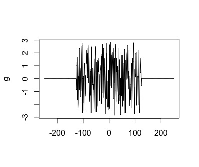
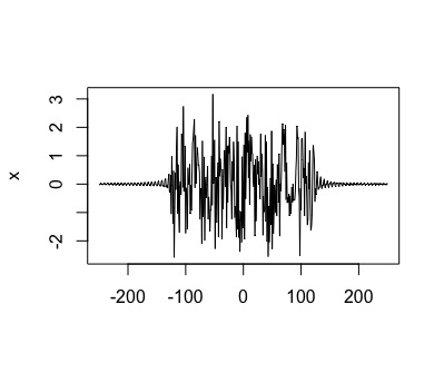
Let us illustrate this on the case of two-step prediction, i.e. prediction of $x(2)$ given truncated observations $\{x(t)\}_{t/2\in{\mathbb{Z}},-T\leq t\leq 0\ }$ for $x\in{\cal V}_{4,\pi}(0.5)$. In our notations, this means that $n=2$ and $\widehat{x}(0)$ is the estimate of $x(2)$. To create a process $x$, we created first a path $\{g(t)\}_{t=-T}^{T}$ generated as a path of a Gaussian stationary process, and we considered $x={\cal Z}^{-1}({\mathbb{I}}_{J_{4,\pi}(\delta)}\left(e^{i\omega}\right)G\left(e^{i\omega}\right))$ for $\delta=0.5$, where $G={\cal Z}g$; by the definitions, it follows that $x\in{\cal V}_{4,\pi}(0.5)$. Figure 5 shows the path of $g$, and Figure 3 shows the path of $x$.

We calculated the relative errors

$$E=\frac{|\widehat{x}(0)-x(2)|}{\sqrt{\frac{1}{T+1}\sum_{t=-T}^{0}x(t)^{2}}}.$$

In particular, for $T=250$ and $\widehat{r}=1.2$, we have that

1. $E=-0.57$ for $\gamma=3$;

2. $E=-0.036$ for $\gamma=10$;

3. $E=-0.027$ for $\gamma=20$.

Figure 1: The distance $|\widehat{H}_{4}\left(e^{i\omega}\right)-e^{2i\omega}|$ for $\gamma=3$ on $[-\pi,\pi]$.

Figure 2: The distance $|\widehat{H}_{4}\left(e^{i\omega}\right)-e^{2i\omega}|$ for $\gamma=3$ on a interior interval inside $(-\pi/4,\pi/4)$.

Figure 3: The distance $|\widetilde{H}_{4}\left(e^{i\omega}\right)-e^{2i\omega}|$ for $\gamma=3$ on $[-\pi,\pi]$.

Figure 4: Process $g$: a truncated path a Gaussian process.

Figure 5: $x={\cal Z}^{-1}({\mathbb{I}}_{J_{4,\beta}(\delta)}\left(e^{i\omega}\right)G\left(e^{i\omega}\right))$, $G={\cal Z}g$.

References

- [1] Dokuchaev, N. (2012). Predictors for discrete time processes with energy decay on higher frequencies. IEEE Transactions on Signal Processing 60, No. 11, 6027-6030.
- [2] Dokuchaev, N, Hin, L.-Y. (2016). On predictability of ultra short AR(1) sequences. Working paper arXiv:1608.08825.
- [3] Dokuchaev, N. (2016). On sampling theorem with sparse decimated samples: exploring branching spectrum degeneracy. arXiv: https://arxiv.org/abs/1605.00414.
- [4] Oppenheim, A., and Schafer, R. (1998). Discrete-Time Signal Processing. Englewood Cliffs, NJ: Prentice-Hall, 2nd ed.
- [5] Serpedin, E Subsequence based recovery of missing samples in oversampled bandlimited signals. (2000). IEEE Transactions on Signal Processing 48(2):580 - 583.