Sampled-data reachability analysis
using sensitivity and mixed-monotonicity

Abstract

This paper over-approximates the reachable sets of a continuous-time uncertain system using the sensitivity of its trajectories with respect to initial conditions and uncertain parameters. We first prove the equivalence between an existing over-approximation result based on the sign-stability of the sensitivity matrices and a discrete-time approach relying on a mixed-monotonicity property. We then present a new over-approximation result which scales at worst linearly with the state dimension and is applicable to any continuous-time system with bounded sensitivity. Finally, we provide a simulation-based approach to estimate these bounds through sampling and falsification. The results are illustrated with numerical examples on traffic networks and satellite orbits.

I Introduction

Reachability analysis deals with the problem of computing the set of all possible successors of a system given its sets of initial conditions and admissible disturbance and uncertainty values (see e.g. [4, 15]). Since exact computation of the reachable set is rarely possible, we instead evaluate an over-approximation to guarantee that the obtained set contains all possible successors of the system. Various methods and representations exist for these over-approximations, including ellipsoids [13], polytopes [5], zonotopes [2], level-sets [14] and unions of intervals [10]. Their main focus is on obtaining over-approximations as close as possible to the actual reachable set, which can then be used for safety verification to ensure that a bad set is never crossed (see e.g. [9]).

Alternatively, methods using a single interval such as [16] focus less on the quality of the over-approximations and more on the simplicity of implementation, including features such as low memory usage (only two states) and low complexity of the reachability analysis (at best constant for monotone systems [3], at worst linear in the state dimension [18]). These properties are particularly important in the context of abstraction-based control synthesis (see, e.g., [7]) where a large number of over-approximations have to be computed, stored and intersected with other intervals.

This paper focuses on the computation of interval over-approximations of reachable sets for a continuous-time uncertain system. As opposed to monotonicity-based approaches relying on the sign of the Jacobian matrices [16, 7], the proposed approach uses the sensitivity matrices (partial derivatives of the system trajectories with respect to the initial state or uncertain parameters). Such an approach was introduced in [18] for the case of systems whose sensitivity matrix is sign-stable over the set of initial states.

This paper presents three main contributions. 1) In Section III, we prove the equivalence between the sign-stable sensitivity approach in [18] for continuous-time systems and the one based on mixed-monotonicity for discrete-time systems in [7]. 2) We next propose in Section IV a generalized sensitivity-based reachability analysis applicable to any continuous-time system whose sensitivity matrices are bounded. This generalization is motivated by the one introduced in [19] for continuous-time mixed-monotone systems. 3) Since the proposed approach is based on the system trajectories and sensitivity, which are unknown for most continuous-time systems, we lastly present a simulation-based method to estimate the sensitivity bounds using sampling and falsification in Section V. Section VI then illustrates these results through an example of traffic flow on a road network and an example of a satellite orbit.

II Problem formulation

Let $\mathbb{R}$ be the set of reals and $\mathcal{I}\subseteq 2^{\mathbb{R}}$ the set of closed real intervals, i.e., for all $X\in\mathcal{I}$, there exist $\underline{x},\overline{x}\in\mathbb{R}$ such that $X=[\underline{x},\overline{x}]=\{x\in\mathbb{R}~{}|~{}\underline{x}\leq x\leq\overline{x}\}\subseteq\mathbb{R}$. $\mathcal{I}^{n}$ and $\mathcal{I}^{n\times q}$ then represent the sets of interval vectors in $\mathbb{R}^{n}$ and interval matrices in $\mathbb{R}^{n\times q}$, respectively.

We consider a continuous-time, time-varying system

$$\dot{x}=f(t,x,p),$$ (1)

with state $x\in\mathbb{R}^{n}$, uncertain parameter $p\in\mathbb{R}^{q}$ and continuously differentiable vector field $f:\mathbb{R}\times\mathbb{R}^{n}\times\mathbb{R}^{q}\rightarrow\mathbb{R}^{n}$. We denote as $\Phi(t;t_{0},x_{0},p)\in\mathbb{R}^{n}$ the state reached by (1) at time $t\geq t_{0}$ from initial state $x_{0}$ with parameter $p$. The variable $p$ can also represent control or disturbance parameters that remain constant over the considered time interval $[t_{0},t]$. Given sets $X_{0}\subseteq\mathbb{R}^{n}$ and $P\subseteq\mathbb{R}^{q}$ of initial states and parameters, respectively, the reachable set of (1) at time $t\geq t_{0}$ is denoted as

$$R(t;t_{0},X_{0},P)=\{\Phi(t;t_{0},x_{0},p)~{}|~{}x_{0}\in X_{0},~{}p\in P\}.$$ (2)

The sensitivity of the trajectories of (1) with respect to the initial conditions and parameters are defined as

$$s^{x}(t;t_{0},x_{0},p)=\frac{\partial\Phi(t;t_{0},x_{0},p)}{\partial x_{0}}\in\mathbb{R}^{n\times n},$$ (3)

$$s^{p}(t;t_{0},x_{0},p)=\frac{\partial\Phi(t;t_{0},x_{0},p)}{\partial p}\in\mathbb{R}^{n\times q}.$$ (4)

The sensitivities defined in (3) and (4) thus represent the differential influence of the initial conditions and parameters, respectively, on the successor of (1) at time $t$.

Our objective is to compute an over-approximation of the reachable set (2) at time $T\geq t_{0}$ for intervals of initial conditions $X_{0}\subseteq\mathbb{R}^{n}$ and of possible parameters $P\subseteq\mathbb{R}^{q}$.

Problem 1.

Given times $t_{0}\in\mathbb{R}$ and $T\geq t_{0}$ and intervals $X_{0}\in\mathcal{I}^{n}$ and $P\in\mathcal{I}^{q}$, find a set $\bar{R}(T;t_{0},X_{0},P)\subseteq\mathbb{R}^{n}$ such that $R(T;t_{0},X_{0},P)\subseteq\bar{R}(T;t_{0},X_{0},P)$.

III Reachability with sign-stable sensitivity

In this section, we review the over-approximation approach presented in [18] with the aim of connecting it in Section III-B to discrete-time mixed-monotonicity from [7].

III-A Sensitivity-based reachability analysis

Reference [18] provides a method to obtain an interval over-approximation of the reachable set for an autonomous system $\dot{x}=f(x)$ whose sensitivity matrix $s^{x}(T,x_{0})$ at time $T\geq 0$ is sign-stable over the set of initial states $X_{0}$. For the purpose of the comparison in Section III-B, these results are reviewed here in a more general framework where the system (1) depends on both time and an uncertain parameter.

We assume that the sensitivity matrices defined in (3) and (4) at time $T$ are sign-stable over the sets $X_{0}$ and $P$, i.e. their entries do not change sign when the initial state and parameter vary in $X_{0}$ and $P$. This is formalized as follows.

Assumption 2.

For all $x_{0},\tilde{x}_{0}\in X_{0}$, $p,\tilde{p}\in P$, $i,j\in\{1,\dots,n\}$, $k\in\{1,\dots,q\}$, we have

$$\begin{cases}s^{x}_{ij}(T;t_{0},x_{0},p)s^{x}_{ij}(T;t_{0},\tilde{x}_{0},\tilde{p})\geq 0,\\ s^{p}_{ik}(T;t_{0},x_{0},p)s^{p}_{ik}(T;t_{0},\tilde{x}_{0},\tilde{p})\geq 0.\end{cases}$$

As $X_{0}$ and $P$ are intervals, let $\underline{x_{0}},\overline{x_{0}}\in\mathbb{R}^{n}$ and $\underline{p},\overline{p}\in\mathbb{R}^{q}$ be such that $X_{0}=[\underline{x_{0}},\overline{x_{0}}]$ and $P=[\underline{p},\overline{p}]$. For each $i\in\{1,\dots,n\}$, define states $\underline{\xi}^{i},\overline{\xi}^{i}\in X_{0}$ (with, e.g., $\underline{\xi}^{i}=[\underline{\xi}^{i}_{1};\dots;\underline{\xi}^{i}_{n}]$) and parameters $\underline{\pi}^{i},\overline{\pi}^{i}\in P$ as diagonally opposite vertices of $X_{0}$ and $P$, respectively, where for each $j\in\{1,\dots,n\}$ (resp. $k\in\{1,\dots,q\}$), their entries $\underline{\xi}^{i}_{j}$, $\overline{\xi}^{i}_{j}$ (resp. $\underline{\pi}^{i}_{k}$, $\overline{\pi}^{i}_{k}$) are allocated to $\underline{x_{0}}_{j}$ or $\overline{x_{0}}_{j}$ (resp. $\underline{p}_{k}$ or $\overline{p}_{k}$) based on the sign of the sensitivity $s^{x}_{ij}$ (resp. $s^{p}_{ik}$):

$$(\underline{\xi}^{i}_{j},\overline{\xi}^{i}_{j})=\begin{cases}(\underline{x_{0}}_{j},\overline{x_{0}}_{j})&\text{ if }s^{x}_{ij}(T;t_{0},x_{0},p)\geq 0,\\ (\overline{x_{0}}_{j},\underline{x_{0}}_{j})&\text{ if }s^{x}_{ij}(T;t_{0},x_{0},p)<0,\\ \end{cases}$$ (5)

$$(\underline{\pi}^{i}_{k},\overline{\pi}^{i}_{k})=\begin{cases}(\underline{p}_{k},\overline{p}_{k})&\text{ if }s^{p}_{ik}(T;t_{0},x_{0},p)\geq 0,\\ (\overline{p}_{k},\underline{p}_{k})&\text{ if }s^{p}_{ik}(T;t_{0},x_{0},p)<0.\end{cases}$$

From (5) and the sensitivity definitions in (3) and (4), the successor $\Phi(T;t_{0},\underline{\xi}^{i},\underline{\pi}^{i})$ (resp. $\Phi(T;t_{0},\overline{\xi}^{i},\overline{\pi}^{i})$) is guaranteed to define the lower bound (resp. upper bound) of the reachable set $R(T;t_{0},X_{0},P)$ on dimension $i$.

Lemma 3 ([18]).

Under Assumption 2, an over-approximation $\bar{R}(T;t_{0},X_{0},P)\in\mathcal{I}^{n}$ of the reachable set is given in each dimension $i\in\{1,\dots,n\}$ by

$$\bar{R}_{i}(T;t_{0},X_{0},P)=[\Phi_{i}(T;t_{0},\underline{\xi}^{i},\underline{\pi}^{i}),\Phi_{i}(T;t_{0},\overline{\xi}^{i},\overline{\pi}^{i})]\in\mathcal{I}.$$

Remark 4.

Lemma 3 requires computing the full successor $\Phi$ of (1) for each pair $(\underline{\xi}^{i},\underline{\pi}^{i}),(\overline{\xi}^{i},\overline{\pi}^{i})\in X_{0}\times P$ even though only the $i^{th}$ entry $\Phi_{i}$ is used in the over-approximation. More than one entry of a successor $\Phi$ may be used when there exists less than $2n$ distinct pairs. The computational burden can thus go from at most $2n$ successors when all the above pairs are distinct, to at least $2$ successors when there exist $\tilde{x},\hat{x}\in X_{0}$ and $\tilde{p},\hat{p}\in P$ such that $(\underline{\xi}^{i},\overline{\xi}^{i},\underline{\pi}^{i},\overline{\pi}^{i})=(\tilde{x},\hat{x},\tilde{p},\hat{p})$ or $(\underline{\xi}^{i},\overline{\xi}^{i},\underline{\pi}^{i},\overline{\pi}^{i})=(\hat{x},\tilde{x},\hat{p},\tilde{p})$ for all $i\in\{1,\dots,n\}$. The latter case corresponds to continuous-time monotonicity of (1) with respect to orthants, as described in [3].

Note also that the over-approximation obtained in Lemma 3 is tight in the sense that $\bar{R}(T;t_{0},X_{0},P)$ is the smallest interval in $\mathcal{I}^{n}$ containing the reachable set.

Corollary 5.

For all $X\in\mathcal{I}^{n}$, if $R(T;t_{0},X_{0},P)\subseteq X$ then $\bar{R}(T;t_{0},X_{0},P)\subseteq X$.

Proof.

For all $i\in\{1,\dots,n\}$ we have $\underline{\xi}^{i},\overline{\xi}^{i}\in X_{0}$ and $\underline{\pi}^{i},\overline{\pi}^{i}\in P$ from (5), thus leading to $\Phi(T;t_{0},\underline{\xi}^{i},\underline{\pi}^{i})\in R(T;t_{0},X_{0},P)$ and $\Phi(T;t_{0},\overline{\xi}^{i},\overline{\pi}^{i})\in R(T;t_{0},X_{0},P)$. Since components $i$ of these reachable states define $\bar{R}_{i}(T;t_{0},X_{0},P)$ in Lemma 3, any interval $X\in\mathcal{I}^{n}$ strictly contained in $\bar{R}(T;t_{0},X_{0},P)$ cannot contain the whole reachable set $R(T;t_{0},X_{0},P)$. ∎

III-B Comparison with discrete-time mixed-monotonicity

In this section, we show that the approach described in Section III-A for the over-approximation of continuous-time systems with sign-stable sensitivity is equivalent to the method presented in [7] for discrete-time systems satisfying a mixed-monotonicity property. A mixed-monotone system $x^{+}=F(t,x,p)$ is one that is decomposable into its increasing and decreasing components and can be characterized as having sign-stable Jacobian matrices $\partial F/\partial x$ and $\partial F/\partial p$. The reader is referred to [7] for the formal definition of a mixed-monotone system and its over-approximation method.

Theorem 6.

Under Assumption 2 and given the discrete-time system $x^{+}=F(t,x,p)$ with $F(t,x,p)=\Phi(T;t,x,p)$, the over-approximations of $R(T;t_{0},X_{0},P)$ in Lemma 3 and of $F(t_{0},X_{0},P)$ in [7] are equivalent.

Proof.

The sign-stability in Assumption 2 implies that $x^{+}=F(t,x,p)$ is mixed-monotone as in [7]. The equivalence then follows from the facts that both methods result in a tight interval over-approximation of the reachable set $F(t_{0},X_{0},P)=R(T;t_{0},X_{0},P)$ ([7, Proposition 2] and Corollary 5) and such tight interval is uniquely defined. ∎

IV Reachability with bounded sensitivity

We now extend the over-approximation method described in (5) and Lemma 3 after relaxing Assumption 2. The new assumption (formalized below) is very mild as it now only requires each entry of the sensitivity matrices at time $T$ to lie in a bounded interval when the initial state and parameter vary in $X_{0}$ and $P$. Unlike Assumption 2, each of these intervals is allowed to contain the value $0$ in its interior. This modification is motivated by an extension of the definition of mixed-monotonicity for continuous-time systems in [19].

Assumption 7.

For all $i,j\in\{1,\dots,n\}$, $k\in\{1,\dots,q\}$, there exist $\underline{s^{x}_{ij}},\overline{s^{x}_{ij}},\underline{s^{p}_{ik}},\overline{s^{p}_{ik}}\in\mathbb{R}$ such that for all $x_{0}\in X_{0}$, $p\in P$ we have $s^{x}_{ij}(T;t_{0},x_{0},p)\in[\underline{s^{x}_{ij}},\overline{s^{x}_{ij}}]$ and $s^{p}_{ik}(T;t_{0},x_{0},p)\in[\underline{s^{p}_{ik}},\overline{s^{p}_{ik}}]$.

Since $X_{0}$ and $P$ are bounded sets, Assumption 7 is naturally satisfied by any system whose trajectory function $\Phi$ is continuously differentiable in its initial state and parameter.

Denoting the center of $[\underline{s^{x}_{ij}},\overline{s^{x}_{ij}}]$ and $[\underline{s^{p}_{ik}},\overline{s^{p}_{ik}}]$ as $s^{x*}_{ij}$ and $s^{p*}_{ik}$, respectively, we update the definition of the states $\underline{\xi}^{i},\overline{\xi}^{i}\in X_{0}$ and parameters $\underline{\pi}^{i},\overline{\pi}^{i}\in P$ in (5) by replacing the right-hand side conditions on the sign of the sensitivity by the same conditions on the center of the sensitivity bounds:

$$(\underline{\xi}^{i}_{j},\overline{\xi}^{i}_{j})=\begin{cases}(\underline{x_{0}}_{j},\overline{x_{0}}_{j})&\text{ if }s^{x*}_{ij}\geq 0,\\ (\overline{x_{0}}_{j},\underline{x_{0}}_{j})&\text{ if }s^{x*}_{ij}<0,\\ \end{cases}$$ (6)

$$(\underline{\pi}^{i}_{k},\overline{\pi}^{i}_{k})=\begin{cases}(\underline{p}_{k},\overline{p}_{k})&\text{ if }s^{p*}_{ik}\geq 0,\\ (\overline{p}_{k},\underline{p}_{k})&\text{ if }s^{p*}_{ik}<0.\end{cases}$$

Note that the condition $s^{x*}_{ij}\geq 0$ in the first line of (6) covers both cases where the whole interval $[\underline{s^{x}_{ij}},\overline{s^{x}_{ij}}]$ is positive (as in (5)) and where it is mostly positive ($\underline{s^{p}_{ik}}\leq 0\leq s^{x*}_{ij}\leq\overline{s^{p}_{ik}}$).

To account for the deviations from the sign-stable cases of (5) that may arise through the mostly positive and mostly negative cases in (6), we introduce two row vectors $c^{i}=[c^{i}_{1},\dots,c^{i}_{n}]\in\mathbb{R}^{n}$ and $d^{i}=[d^{i}_{1},\dots,d^{i}_{q}]\in\mathbb{R}^{q}$ for each $i\in\{1,\dots,n\}$ defined by, for all $j\in\{1,\dots,n\}$, $k\in\{1,\dots,q\}$,

$$c^{i}_{j}=\begin{cases}\min(0,\underline{s^{x}_{ij}})&\text{ if }s^{x*}_{ij}\geq 0,\\ \max(0,\overline{s^{x}_{ij}})&\text{ if }s^{x*}_{ij}<0,\\ \end{cases}$$ (7)

$$d^{i}_{k}=\begin{cases}\min(0,\underline{s^{p}_{ik}})&\text{ if }s^{p*}_{ik}\geq 0,\\ \max(0,\overline{s^{p}_{ik}})&\text{ if }s^{p*}_{ik}<0.\end{cases}$$

Equation (7) means that $c^{i}_{j}=0$ in the sign-stable cases, $c^{i}_{j}=\underline{s^{x}_{ij}}\leq 0$ in the mostly positive case and $c^{i}_{j}=\overline{s^{x}_{ij}}\geq 0$ in the mostly negative case.

Without the sign-stability from Assumption 2, the successors $\Phi_{i}(T;t_{0},\underline{\xi}^{i},\underline{\pi}^{i})$ and $\Phi_{i}(T;t_{0},\overline{\xi}^{i},\overline{\pi}^{i})$ are not guaranteed to over-approximate dimension $i$ of the reachable set. To compute an interval that is guaranteed to over-approximate the reachable set, the generalization of Lemma 3 thus requires the addition of compensation terms as in the result below, where $\underline{\xi}^{i},\overline{\xi}^{i}\in\mathbb{R}^{n}$ and $\underline{\pi}^{i},\overline{\pi}^{i}\in\mathbb{R}^{q}$ are column vectors and $c^{i}\in\mathbb{R}^{n}$ and $d^{i}\in\mathbb{R}^{q}$ are row vectors.

Theorem 8.

Under Assumption 7, an over-approximation $\bar{R}(T;t_{0},X_{0},P)\in\mathcal{I}^{n}$ is given in each dimension $i\in\{1,\dots,n\}$ by:

$$\bar{R}_{i}(T;t_{0},X_{0},P)=\\ [\Phi_{i}(T;t_{0},\underline{\xi}^{i},\underline{\pi}^{i})-c^{i}(\underline{\xi}^{i}-\overline{\xi}^{i})-d^{i}(\underline{\pi}^{i}-\overline{\pi}^{i}),\\ \Phi_{i}(T;t_{0},\overline{\xi}^{i},\overline{\pi}^{i})+c^{i}(\underline{\xi}^{i}-\overline{\xi}^{i})+d^{i}(\underline{\pi}^{i}-\overline{\pi}^{i})].$$

Proof.

Consider an auxiliary system whose trajectories $\hat{\Phi}$ are such that for all $x_{0}\in X_{0}$, $p\in P$ and $i\in\{1,\dots,n\}$ we have $\hat{\Phi}_{i}(T;t_{0},x_{0},p)=\Phi_{i}(T;t_{0},x_{0},p)-c^{i}x_{0}-d^{i}p$. Then, from the sensitivity bounds in Assumption 7 and the definition of $c^{i}$ and $d^{i}$ in (7), the sensitivities $\hat{s}^{x}(T;t_{0},x_{0},p)$ and $\hat{s}^{p}(T;t_{0},x_{0},p)$ of this auxiliary system are sign-stable over the sets $X_{0}$ and $P$, i.e. for all $x_{0}\in X_{0}$ and $p\in P$, $\hat{s}^{x}_{ij}(T;t_{0},x_{0},p)=s^{x}_{ij}(T;t_{0},x_{0},p)-c^{i}_{j}\geq 0$ (resp. $\leq 0$) if $s^{x*}_{ij}\geq 0$ (resp. $\leq 0$), with similar results for $\hat{s}^{p}$. Since $\hat{s}^{x}_{ij}(T;t_{0},x_{0},p)$ and $s^{x*}_{ij}$ have the same sign (and similarly for $\hat{s}^{p}_{ij}(T;t_{0},x_{0},p)$ and $s^{p*}_{ij}$), this also guarantees that the states $\underline{\xi}^{i},\overline{\xi}^{i}\in X_{0}$ and parameters $\underline{\pi}^{i},\overline{\pi}^{i}\in P$ obtained in (6) are the same as their hatted counterparts that would be obtained in (5) for the auxiliary system. Applying Lemma 3 to $\hat{\Phi}$ implies that for all $i\in\{1,\dots,n\}$, $x_{0}\in X_{0}$ and $p\in P$,

$$\Phi_{i}(T;t_{0},x_{0},p)\in\\ [\Phi_{i}(T;t_{0},\underline{\xi}^{i},\underline{\pi}^{i})+c^{i}(x_{0}-\underline{\xi}^{i})+d^{i}(p-\underline{\pi}^{i}),\\ \Phi_{i}(T;t_{0},\overline{\xi}^{i},\overline{\pi}^{i})+c^{i}(x_{0}-\overline{\xi}^{i})+d^{i}(p-\overline{\pi}^{i})].$$

From (7), $c^{i}_{j}\leq 0$ (resp. $\geq 0$) if $s^{x*}_{ij}\geq 0$ (resp. $\leq 0$). Then for all $x_{0}\in[\underline{x_{0}},\overline{x_{0}}]$, we have $c^{i}\overline{\xi}^{i}\leq c^{i}x_{0}\leq c^{i}\underline{\xi}^{i}$, with $\underline{\xi}^{i},\overline{\xi}^{i}\in X_{0}$ defined as in (6). We similarly obtain $d^{i}\overline{\pi}^{i}\leq d^{i}p\leq d^{i}\underline{\pi}^{i}$ for all $p\in[\underline{p},\overline{p}]$, which finally leads to the over-approximation in the theorem statement. ∎

Remark 9.

Unlike the sign-stable case (Lemma 3, Corollary 5), tightness of the over-approximation $\bar{R}(T;t_{0},X_{0},P)$ cannot be guaranteed in the general case of Theorem 8 due to the additional terms $\pm c^{i}(\underline{\xi}^{i}-\overline{\xi}^{i})$ and $\pm d^{i}(\underline{\pi}^{i}-\overline{\pi}^{i})$.

Following the comparison with discrete-time mixed-monotonicity in Section III-B, a side product of Theorem 8 is a new over-approximation method for discrete-time systems generalizing the approach from [7].

Corollary 10.

Let $x^{+}=F(t,x,p)$ have bounded Jacobian matrices $\frac{\partial F(t,x,p)}{\partial x}\in\mathcal{I}^{n\times n}$ and $\frac{\partial F(t,x,p)}{\partial p}\in\mathcal{I}^{n\times q}$ over all states $x\in[\underline{x_{0}},\overline{x_{0}}]$ and parameters $p\in[\underline{p},\overline{p}]$. Then the reachable set $F(t,X_{0},P)$ after one step can be over-approximated as follows in each dimension $i\in\{1,\dots,n\}$:

$$F_{i}(t,X_{0},P)\subseteq[F_{i}(t,\underline{\xi}^{i},\underline{\pi}^{i})-c^{i}(\underline{\xi}^{i}-\overline{\xi}^{i})-d^{i}(\underline{\pi}^{i}-\overline{\pi}^{i}),\qquad\\ F_{i}(t,\overline{\xi}^{i},\overline{\pi}^{i})+c^{i}(\underline{\xi}^{i}-\overline{\xi}^{i})+d^{i}(\underline{\pi}^{i}-\overline{\pi}^{i})],$$

where $\underline{\xi}^{i},\overline{\xi}^{i},\underline{\pi}^{i},\overline{\pi}^{i}$ and $c^{i},d^{i}$ are defined as in (6) and (7) using the bounds of the Jacobian matrices.

V Obtaining bounds on the sensitivities

The approach presented above relies on the trajectory $\Phi(\cdot;t_{0},x_{0},p):[t_{0},+\infty)\rightarrow X$ evaluated at time $T\geq t_{0}$, which is rarely known explicitly. Although the successors $\Phi(T;t_{0},x_{0},p)$ can be computed through numerical integration of the system $\dot{x}=f(t,x,p)$, the main challenge is the computation of the sensitivity matrices $s^{x}(T;t_{0},x_{0},p)$ in (3) and $s^{p}(T;t_{0},x_{0},p)$ in (4) for all $x_{0}\in X_{0}$ and $p\in P$ to evaluate the sign-stability or boundedness of these sensitivities as in Assumptions 2 and 7, respectively.

V-A Sampling and falsification

In this section, we propose a simulation-based approach where we first evaluate the sensitivity bounds from a few samples in $X_{0}\times P$ and then use a falsification method to iteratively enlarge these bounds by looking for other pairs in $X_{0}\times P$ whose sensitivity does not belong to these bounds.

From the definition of $s^{x}$ in (3), we can use the chain rule to define the time-varying linear system

$$\dot{s}^{x}(t;t_{0},x_{0},p)=D_{f}^{x}|_{\Phi}s^{x}(t;t_{0},x_{0},p),$$ (8)

where $D_{f}^{x}|_{\Phi}=D_{f}^{x}(t,\Phi(t;t_{0},x_{0},p),p)$ denotes the Jacobian $D_{f}^{x}(t,x,p)=\frac{\partial f(t,x,p)}{\partial x}$ evaluated along the trajectory $\Phi(t;t_{0},x_{0},p)$. System (8) is initialized with the identity matrix $s^{x}(t_{0};t_{0},x_{0},p)=I_{n}\in\mathbb{R}^{n\times n}$ [8]. A similar time-varying affine system can be found for the sensitivity $s^{p}$:

$$\dot{s}^{p}(t;t_{0},x_{0},p)=D_{f}^{x}|_{\Phi}s^{p}(t;t_{0},x_{0},p)+D_{f}^{p}|_{\Phi},$$ (9)

where $D_{f}^{p}|_{\Phi}$ is the evaluation of $D_{f}^{p}(t,x,p)=\frac{\partial f(t,x,p)}{\partial p}$ along the trajectory $\Phi(t;t_{0},x_{0},p)$ and (9) is initialized with the zero matrix $s^{p}(t_{0};t_{0},x_{0},p)=0_{n\times q}\in\mathbb{R}^{n\times q}$ [12].

For a given time $T\geq t_{0}$, we first compute the sensitivity matrices $s^{x}(T;t_{0},x_{0},p)$ and $s^{p}(T;t_{0},x_{0},p)$ through the numerical integration of the systems (8) and (9) for at least one pair $(x_{0},p)\in X_{0}\times P$ to obtain initial sensitivity bounds denoted as $[\underline{s^{x}},\overline{s^{x}}]\in\mathcal{I}^{n\times n}$ and $[\underline{s^{p}},\overline{s^{p}}]\in\mathcal{I}^{n\times q}$. More than one pair $(x_{0},p)$ can be obtained through either random sampling or a gridded discretization of $X_{0}\times P$.

The second step aims to falsify these bounds [11] through an optimization problem, i.e. to find $x_{0}\in X_{0}$ and $p\in P$ such that either $s^{x}(T;t_{0},x_{0},p)\notin[\underline{s^{x}},\overline{s^{x}}]$ or $s^{p}(T;t_{0},x_{0},p)\notin[\underline{s^{p}},\overline{s^{p}}]$. Focusing on the sensitivity with respect to the initial state, we want to solve the following optimization problem

$$\min_{\begin{subarray}{c}x_{0}\in X_{0}\\ p\in P\end{subarray}}\left(\min_{i,j}\left(\frac{\overline{s^{x}_{ij}}-\underline{s^{x}_{ij}}}{2}-\left|s^{x}_{ij}(T;t_{0},x_{0},p)-s_{ij}^{x*}\right|\right)\right),$$

where for each pair $(i,j)$ we consider a negative absolute value function centered on $s_{ij}^{x*}$ and translated such that the global cost function is negative if and only if there exist $i,j\in\{1,\dots,n\}$ such that $s^{x}_{ij}(T;t_{0},x_{0},p)\notin[\underline{s^{x}_{ij}},\overline{s^{x}_{ij}}]$. If the obtained local minimum is negative and the corresponding arguments are denoted as $x_{0}^{*}\in X_{0}$ and $p^{*}\in P$, the sensitivity bounds are updated as: $\underline{s^{x}}\leftarrow\min(\underline{s^{x}},s^{x}(T;t_{0},x_{0}^{*},p^{*}))$, $\overline{s^{x}}\leftarrow\max(\overline{s^{x}},s^{x}(T;t_{0},x_{0}^{*},p^{*}))$, using elementwise $\min$ and $\max$ operators. This process is repeated with the new bounds until a positive minimum is obtained. A similar approach is applied to $[\underline{s^{p}},\overline{s^{p}}]$.

Remark 11.

While this approach is likely to result in an accurate approximation of the actual sensitivity bounds, it is not guaranteed to over-approximate the set of all possible sensitivity values over $X_{0}\times P$ since the falsification relies on an optimization problem only able to provide local minima.

V-B Interval arithmetics

An alternative approach recommended in [18] is based on the use of interval arithmetics to solve an affine time-varying system as presented in [1]. For the purpose of comparison with the method in Section V-A on the numerical examples of Section VI, we give an overview of how the results described in [1] can be applied to the sensitivity systems (8) and (9) to obtain guaranteed bounds on the sensitivity matrices. We start from the assumption that bounds on the Jacobian matrices $D_{f}^{x}(t,x,p)=\frac{\partial f(t,x,p)}{\partial x}$ and $D_{f}^{p}(t,x,p)=\frac{\partial f(t,x,p)}{\partial p}$ of (1) are known or can be computed.

Assumption 12.

Given an invariant set $X\subseteq\mathbb{R}^{n}$ of (1), there exist interval matrices $\mathcal{A}\in\mathcal{I}^{n\times n}$ and $\mathcal{B}\in\mathcal{I}^{n\times q}$ such that for all $t\in[t_{0},+\infty)$, $x\in X$, $p\in P$, we have $D_{f}^{x}(t,x,p)\in\mathcal{A}$ and $D_{f}^{p}(t,x,p)\in\mathcal{B}$.

We can then rewrite (8) and (9) as the set-valued systems

$$\dot{s}^{x}(t)\in\mathcal{A}s^{x}(t), s^{x}(t_{0})=I_{n},$$ (10)

$$\dot{s}^{p}(t)\in\mathcal{A}s^{p}(t)+\mathcal{B}, s^{p}(t_{0})=0_{n\times q}.$$ (11)

The solution of these systems at time $T$ is over-approximated using interval arithmetics and a truncated Taylor series of the interval matrix exponential $e^{\mathcal{A}(T-t_{0})}\in\mathcal{I}^{n\times n}$, detailed in [1].

Lemma 13 ([1]).

Under Assumption 12, there exist functions $m:[0,+\infty)\rightarrow\mathbb{N}$ and $E:[0,+\infty)\rightarrow\mathcal{I}^{n\times n}$ defined in [1] such that for all $T\geq t_{0}$, we have

$$s^{x}(T)\in\sum_{i=0}^{m(T-t_{0})}\frac{(\mathcal{A}(T-t_{0}))^{i}}{i!}+E(T-t_{0}),$$

$$s^{p}(T)\in\left(\sum_{i=0}^{m(T-t_{0})}\frac{(\mathcal{A}(T-t_{0}))^{i}}{(i+1)!}+E(T-t_{0})\right)(T-t_{0})\mathcal{B}.$$

Remark 14.

Unlike the sampling-based method in Section V-A, Lemma 13 provides guaranteed over-approximations for the sensitivities but risks being overly conservative since interval arithmetics cannot provide exact set computation when more than two interval matrices are multiplied [10].

Remark 15.

The minimal Taylor order $m(T-t_{0})$ for Lemma 13 to hold is a linearly increasing function of the time step $T-t_{0}$ [1]. This approach might thus be practically infeasible when the desired time step $T-t_{0}$ is too large.

VI Numerical examples

All computations are run with Matlab on a laptop with a 1.7GHz CPU and 4GB of RAM.

VI-A Traffic network

Consider the $3$-link traffic network describing a diverge junction (the vehicles in link $1$ divide evenly among the outgoing links $2$ and $3$) inspired by [6]:

$$\dot{x}=\frac{1}{T}\begin{pmatrix}p-g(x)\\ g(x)/2-\min(c,vx_{2})\\ g(x)/2-\min(c,vx_{3})\end{pmatrix},$$ (12)

where $g(x)=\min(c,vx_{1},2w(\bar{x}-x_{2}),2w(\bar{x}-x_{3}))$, $x\in\mathbb{R}^{3}$ is the vehicle density on the three links, $p\in P=[40,60]$ is the constant but uncertain vehicle inflow to link $1$, $T=30$ seconds and $c=40$, $v=0.5$, $\bar{x}=320$, $w=1/6$ are known parameters of the network detailed in [6].

In addition to the uncertain disturbance input $p\in P=[40,60]$, we consider a set $X_{0}\subseteq\mathcal{I}^{3}$ of initial conditions such that $X_{0}=[150,200]\times[250,320]\times[50,100]$, meaning that link $2$ is close to its maximal capacity $\bar{x}=320$ while link $3$ has more availability. Figure 1 presents the projection in the $(x_{1},x_{3})$ plane of the initial interval $X_{0}$ (dashed black), the reachable set $\{\Phi(T;x_{0},p)~{}|~{}x_{0}\in X_{0},p\in P\}$ (hatched black) of (12) after time $T=30$ seconds and two interval over-approximations of this set obtained as described below.

Using the simulation-based approach in Section V-A, we get a first approximation of the sensitivity bounds of (12) from a grid of $16$ samples in $X_{0}\times P$ ($2$ samples per dimension) computed in $0.98$s, which is then refined in $15.8$s through falsification, stopping after $6$ iterations. From these times, it is thus advised to use a finer sampling of $X_{0}\times P$ to obtain a good initial estimation of the sensitivity bounds so that the number of falsification runs is reduced. The numerical computations indicate that the sensitivity bounds for (12) are sign-stable, thus leading to the tight red over-approximation in Figure 1 obtained after applying Lemma 3.

The second over-approximation in green is computed from sensitivity bounds obtained with the interval arithmetics approach in Lemma 13, where the Jacobian bounds as in Assumption 12 are obtained analytically from the dynamics (12). We pick a Taylor order $m=7$ (empirically, we see no improvement on the sensitivity bounds for larger values) which is greater than the minimal value $m(T)=0$ for Lemma 13 to hold. The sensitivity bounds are computed in $14$ms, but as predicted in Remark 14 they are much more conservative than the one obtained in the first approach and they do not satisfy Assumption 2. The over-approximation in green is thus obtained from the generalized result in Theorem 8 and is much larger than the red one, firstly because Theorem 8 is known not to be tight (Remark 9), but also because it tries to compensate for the sensitivity elements believed not to be sign-stable while their real values are actually sign-stable according to the sampling-based estimation above.

The computation of both red and green over-approximations (from Lemma 3 and Theorem 8) is done in $60$ms. The volumes of the red and green over-approximations are respectively $1.7$ and $5.1$ times the volume of the true reachable set.

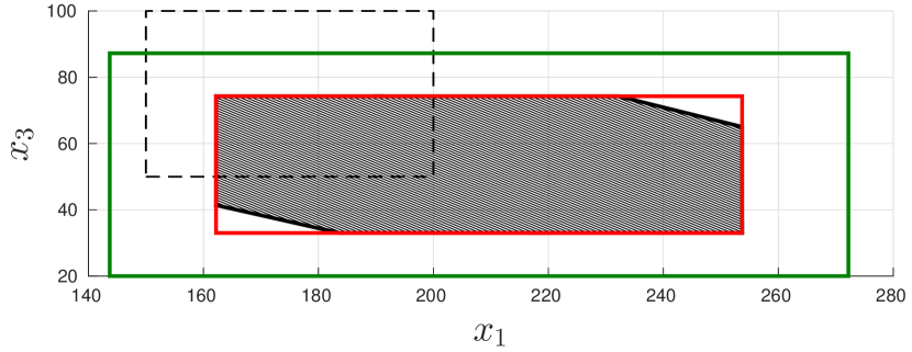
Figure 1: $(x_{1},x_{3})$-projection of the reachable set (hatched black) of (12) from the initial interval (dashed black) and its over-approximations using sampling-based sensitivity bounds (red) and interval arithmetics (green).

To study the scalability of the approach, we now extend this three link example by adding links downstream of the diverging junction so that traffic on link $2$ flows to link $4$ then to link $6$, etc., and, likewise, traffic flows from link $3$ to $5$ to $7$, etc. The modified dynamics are

$$f_{i}(x,p) =\frac{1}{T}(g(x)/2-h(x_{i},x_{i+2})),\ i\in\{2,3\}$$ (13)

$$f_{i}(x,p) =\frac{1}{T}(\beta h(x_{i-2},x_{i})-h(x_{i},x_{i+2})),\ i\in\{4,\ldots,n\}$$ (14)

where $h(\eta,\zeta)=\min\left(c,v\eta,\frac{w}{\beta}(\bar{x}-\zeta)\right)$, $n$ is the total number of links in the network, and we take $\beta=\frac{3}{4}$ ($1-\beta$ is the fraction of vehicles exiting the network after each link). For $i\in\{n-1,n\}$, the term $\frac{w}{\beta}(\bar{x}-x_{i+2})$ is excluded from the minimization in $h$. Considering a $11$-link network with $X_{0}=[20,300]^{11}$, we apply the same methods as for the previous $3$-link case. The sensitivity bounds are first evaluated from a grid of $4096$ samples of $X_{0}\times P$ ($2$ samples per dimension) in $862$s, followed by $3$ iterations of falsification in $21$s, resulting in sign-stable bounds. Another set of bounds is computed in $0.54$s through interval arithmetics with a Taylor order $m=15$, resulting in bounds which are not sign-stable. The over-approximations in the state space (from Lemma 3 and Theorem 8) using both sets of sensitivity bounds are computed in $0.25$s. From the sign-stability assumption, the first interval over-approximation is guaranteed to be tight to the actual reachable set (Corollary 5). On the other hand, the over-approximation obtained from interval arithmetics is not tight and has $68$ times the volume of the first over-approximation, making it too loose for practical use. From the computation times for both the $3$-link and $11$-link models, we note that the approach scales well with the state dimension apart from the main bottleneck in the sampling approach, whose complexity grows exponentially with $n$ for a gridded sampling.

VI-B Satellite orbit

Consider the non-linear system describing a satellite orbiting a celestial body from [17]:

$$\dot{x}=\begin{pmatrix}x_{2}\\ -\frac{p}{x_{1}^{2}}+x_{1}x_{4}^{2}\\ x_{4}\\ -\frac{2x_{2}x_{4}}{x_{1}}\end{pmatrix},\quad x(0)=\begin{pmatrix}R+400\\ 0\\ 0\\ \sqrt{\frac{p}{(R+400)^{3}}}\end{pmatrix},$$ (15)

where $x_{1}$ is the distance of the satellite to the center of the body, $x_{3}$ its angular position and $x_{2}$ and $x_{4}$ their respective derivatives. The parameter $p\in\mathbb{R}$ is defined as $p=GM$, where $G$ is the gravitational constant and $M$ the mass of the body. The initial conditions of (15) are chosen to obtain a circular orbit at $400$km above the body’s surface (radius $R$). Assuming uncertain values (around Earth’s known values) for both the parameter $p\in[3.9779,3.9938]\cdot 10^{5}$ km${}^{3}/$s² and the desired orbit radius $R+400\in[6.7718,6.7845]\cdot 10^{3}$ km, we obtain uncertainty bounds denoted as $p\in P\subseteq\mathbb{R}$ and $x(0)\in X_{0}\in\mathcal{I}\times\{0\}\times\{0\}\times\mathcal{I}\subseteq\mathbb{R}^{4}$.

We want to study the effect of these uncertainties on the reachable set of (15) at time $T=92$ minutes (after approximately one whole revolution around the Earth). As expected from Remark 15, the interval arithmetics result from Lemma 13 is not applicable to (15) since the choice of $T=5520$s requires a minimum Taylor order $m(T)=88883$, which cannot be computed in reasonable time. We thus rely on the sampling-based approach from Section V-A by first evaluating the sensitivity bounds for $100$ random samples in $X_{0}\times P$, obtained in $68$s. A single iteration of falsification is then run in $5$s, meaning that the sampling-based approximation of the bounds already covered all sensitivity values that could be found from the optimization problem solved in the falsification. The obtained sensitivity bounds $[\underline{s^{x}},\overline{s^{x}}]\in\mathcal{I}^{4\times 4}$ and $[\underline{s^{p}},\overline{s^{p}}]\in\mathcal{I}^{4}$ do not satisfy the sign-stability condition in Assumption 2 on $9$ of their $20$ entries, thus requiring the application of the generalized result in Theorem 8 to compute (in $58$ms) the over-approximation of the reachable set of (15) at time $T$, projected into the polar coordinate system $(x_{1},x_{3})$ in Figure 2 (in blue) along with an estimation of the actual reachable set (cloud of black dots) obtained from $10000$ random samples in $X_{0}\times P$. Despite the lack of guarantee in the sampling-based approach (Remark 11), Figure 2 suggests that the computed interval does indeed over-approximate the reachable set and is not overly conservative.

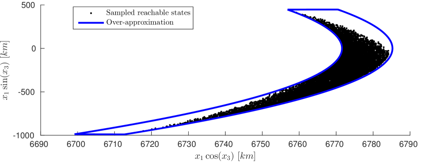
Figure 2: Reachable set (black) of (15) and its over-approximation $\bar{R}(T;0,X_{0},P)$ (blue) projected in the polar plane $(x_{1},x_{3})$.

VII Conclusion

This paper provides a new reachability analysis method based on the sensitivity matrices of a continuous-time system and applicable to the wide class of systems whose sensitivity matrices at a given time are bounded over the sets of uncertain parameters and initial conditions. This assumption is very mild since it is naturally satisfied by any system with a sufficiently smooth trajectory function. The computation of an interval over-approximation of the reachable set using this approach has favorable scalability, since its complexity is at worst linear in the state dimension.

Since the system trajectories or sensitivity matrices are rarely known explicitly, the main challenge of this method lies in obtaining bounds on the sensitivity. Two such approaches are considered in this paper. The first approach relies on interval arithmetics and provides guaranteed sensitivity bounds but can rarely be applied in practice, as the bounds are often overly conservative and the computation is infeasible for larger time steps. The second approach is based on sampling and falsification and provides more reliable values for the sensitivity bounds although without formal guarantees, which may present a risk for safety-critical applications. The sampling-based approach is currently the main computational bottleneck, since the suggested number of samples to obtain a good first estimate of the sensitivity bounds (in order to minimize the number of falsification iterations) grows exponentially with the state dimension.

Future work will aim to exploit these results for abstraction-based synthesis (see e.g. [7]), where a control problem on a differential equation is instead solved on a finite transition system abstracting the continuous dynamics. In such approaches, reachability analysis plays a central role in the creation of the abstraction and intervals are commonly used for their implementation benefits (low memory requirement, easy to check intersection with other intervals).

References

- [1] M. Althoff, O. Stursberg, and M. Buss. Reachability analysis of linear systems with uncertain parameters and inputs. In 46th IEEE Conference on Decision and Control, pages 726–732. IEEE, 2007.
- [2] M. Althoff, O. Stursberg, and M. Buss. Computing reachable sets of hybrid systems using a combination of zonotopes and polytopes. Nonlinear analysis: hybrid systems, 4(2):233–249, 2010.
- [3] D. Angeli and E. D. Sontag. Monotone control systems. IEEE Transactions on Automatic Control, 48(10):1684–1698, 2003.
- [4] F. Blanchini and S. Miani. Set-theoretic methods in control. Springer, 2008.
- [5] A. Chutinan and B. H. Krogh. Computational techniques for hybrid system verification. IEEE transactions on automatic control, 48(1):64–75, 2003.
- [6] S. Coogan and M. Arcak. A benchmark problem in transportation networks. arXiv preprint arXiv:1803.00367.
- [7] S. Coogan and M. Arcak. Efficient finite abstraction of mixed monotone systems. In Proceedings of the 18th International Conference on Hybrid Systems: Computation and Control, pages 58–67. ACM, 2015.
- [8] A. Donzé and O. Maler. Systematic simulation using sensitivity analysis. In International Workshop on Hybrid Systems: Computation and Control, pages 174–189. Springer, 2007.
- [9] G. Frehse. Phaver: Algorithmic verification of hybrid systems past hytech. In International workshop on hybrid systems: computation and control, pages 258–273. Springer, 2005.
- [10] L. Jaulin. Applied interval analysis: with examples in parameter and state estimation, robust control and robotics, volume 1. Springer Science & Business Media, 2001.
- [11] J. Kapinski, J. V. Deshmukh, X. Jin, H. Ito, and K. Butts. Simulation-based approaches for verification of embedded control systems: an overview of traditional and advanced modeling, testing, and verification techniques. IEEE Control Systems, 36(6):45–64, 2016.
- [12] H. K. Khalil. Nonlinear systems. Pearson, third edition, 2001.
- [13] A. A. Kurzhanskiy and P. Varaiya. Ellipsoidal techniques for reachability analysis of discrete-time linear systems. IEEE Transactions on Automatic Control, 52(1):26–38, 2007.
- [14] I. Mitchell and C. J. Tomlin. Level set methods for computation in hybrid systems. In Hybrid Systems: Computation and Control, pages 310–323. Springer, 2000.
- [15] S. V. Rakovic, E. C. Kerrigan, D. Q. Mayne, and J. Lygeros. Reachability analysis of discrete-time systems with disturbances. IEEE Transactions on Automatic Control, 51(4):546–561, 2006.
- [16] N. Ramdani, N. Meslem, and Y. Candau. A hybrid bounding method for computing an over-approximation for the reachable set of uncertain nonlinear systems. IEEE Transactions on Automatic Control, 54(10):2352–2364, 2009.
- [17] W. T. Thomson. Introduction to space dynamics. Courier Corporation, 2012.
- [18] B. Xue, M. Fränzle, and P. N. Mosaad. Just scratching the surface: Partial exploration of initial values in reach-set computation. In 56th IEEE Conference on Decision and Control, pages 1769–1775, 2017.
- [19] L. Yang and N. Ozay. A note on some sufficient conditions for mixed monotone systems. Technical report, 2017.